1 Introduction
Buoyant inflows into basins can have a dominant influence on the density stratification of the basin water column and the pattern of water circulation in the basin (Carmack Reference Carmack1979; Killworth & Carmack Reference Killworth and Carmack1979). Understanding such inflows is important in limnology: they influence the public health risks associated with pollutants entering drinking water reservoirs (Antenucci, Brookes & Hipsey Reference Antenucci, Brookes and Hipsey2005) and the ecological functioning of lakes (Šimek et al. Reference Šimek, Comerma, García, Nedoma, Marcé and Armengol2010). Other significant applications with similar physical mechanisms include meltwater rising into fjords from glacier termini (Wells & Worster Reference Wells and Worster2008; Kerr & McConnochie Reference Kerr and McConnochie2015), circulation of the global ocean (Legg et al. Reference Legg, Ezer, Jackson, Briegleb, Danabasoglu, Large, Wu, Chang, Özgökmen and Peters2009), natural ventilation of buildings (Linden Reference Linden1999) and various industrial flows (Germeles Reference Germeles1975; Seon et al. Reference Seon, Hulin, Salin, Perrin and Hinch2006).
When an inflow of constant density water enters a basin of homogeneous lighter water from a localised source at the top of an inclined boundary, such as when a cold river enters a lake, the inflow travels as an inclined gravity current to the bottom of the basin. An inclined gravity current can be considered a predominantly horizontal motion along a gentle slope, driven by density differences (Simpson Reference Simpson1987). The inflowing water accumulates in a ponded region at the bottom of the basin, establishing a stable density stratification in this lower part of the ambient fluid. Throughout this article, all fluid outside the gravity current is termed the ‘ambient fluid’, both the uniform upper layer and the stratified ponded region. The prevailing model for turbulent, inclined gravity currents supposes that ambient water from the basin is drawn into the gravity current by a unidirectional entrainment process (Killworth & Carmack Reference Killworth and Carmack1979; Turner Reference Turner1986; Dallimore, Hodges & Imberger Reference Dallimore, Hodges and Imberger2003). The fluid in the gravity current is assumed to be mixed such that the current has a homogeneous density profile (Morton, Taylor & Turner Reference Morton, Taylor and Turner1956; Dallimore et al.
Reference Dallimore, Hodges and Imberger2003). This model results in all fluid in the gravity current descending through the ponded region to the bottom of the basin throughout the filling process (Baines & Turner Reference Baines and Turner1969). These models of gravity current fed basins, often used in lakes (Killworth & Carmack Reference Killworth and Carmack1979; Dallimore et al.
Reference Dallimore, Hodges and Imberger2003), are based on the seminal Baines & Turner (Reference Baines and Turner1969) ‘filling box’ model. We term this the persistently entraining model and describe it in § 4.1. Other laboratory work has shown that for inclines ranging from
 $12^{\circ }$
to
 $70^{\circ }$
the ratio
 $E_{eq}$
of the horizontal entrainment velocity to the gravity current velocity is approximately constant with a value of 0.08 (Wells & Wettlaufer Reference Wells and Wettlaufer2005). Other extensions to the Baines & Turner (Reference Baines and Turner1969) model have included the influences of rotation on the gravity current and diffusion in the ambient fluid (Wells & Wettlaufer Reference Wells and Wettlaufer2005; Hughes & Griffiths Reference Hughes and Griffiths2006).
However, later observations have found that, when the ambient fluid is stratified, the exchange flow between the gravity current is not necessarily a unidirectional entrainment into the current (Mitsudera & Baines Reference Mitsudera and Baines1992; Baines Reference Baines2001). In stratified ambient fluid, the outer layers of a gravity current on a shallow slope can separate from the current and move into the ambient fluid (Baines Reference Baines2005; Wells & Wettlaufer Reference Wells and Wettlaufer2007). This allows the possibility of a bidirectional exchange between the gravity current and a continuously stratified ambient fluid over the full length of the gravity current. The flux out of the boundary layer into the ambient fluid is here termed peeling detrainment. This is appropriate because the least dense fluid in the gravity current, in the outer layers neighbouring the ambient fluid, peels away to come to rest in the stratified ambient fluid at a different depth from the remainder of the gravity current fluid. The aim of this paper is to demonstrate how peeling detrainment in the stratified ponded region of a filling basin influences both the transport pathway for the inflow and the stratification that builds up in the basin. The nature of detrainment is not fully understood and is a topic of ongoing study. For example, observations of detrainment behaviours have been reported in continuous stratifications (Wong, Griffiths & Hughes Reference Wong, Griffiths and Hughes2001; Baines Reference Baines2005), layered stratifications (Wells & Wettlaufer Reference Wells and Wettlaufer2007; Cortés, Rueda & Wells Reference Cortés, Rueda and Wells2014b ), rotating experiments (Lane-Serff & Baines Reference Lane-Serff and Baines2000), two-phase plumes (Asaeda & Imberger Reference Asaeda and Imberger1993) and in ocean (Gordon et al. Reference Gordon, Orsi, Muench, Huber, Zambianchi and Visbeck2009) and lake observations (Cortés et al. Reference Cortés, Fleenor, Wells, de Vicente and Rueda2014a ). Detrainment processes are not currently incorporated in numerical models of lakes or oceans, but could play a role in the evolution of the water column in such basins.
In a two-layer ambient stratification, if none of the gravity current fluid is denser than the lower layer, a descending gravity current will form an intrusive gravity current at the pycnocline (Monaghan Reference Monaghan2007). If some of the gravity current is denser than the lower layer, the current will split into two currents with lighter fluid intruding at the pycnocline and the denser fluid penetrating through the pycnocline and continuing to move along the slope (Monaghan Reference Monaghan2007; Cortés et al. Reference Cortés, Rueda and Wells2014b ). Gravity current fluid does not move into the middle of a homogeneous layer because the mixed fluid in the gravity current must either be lighter or denser than a homogeneous layer. In a linear stratification, gravity current fluid moves directly into a continuously stratified ambient fluid over an extended range of depths, because the gravity current – which is itself internally stratified – contains fluid that is neutrally buoyant over a range of depths in the ambient stratification.
Here we report a series of laboratory experiments examining the evolution of the stratification of a basin driven by a dense inflowing gravity current. We incorporate the peeling detrainment phenomenon into a persistently entraining model and predict the stratification that develops in the basin. We compare both the old persistently entraining model and the new peeling detrainment model with the experiments, finding the observations compare much better with our new model. From these results, we conclude that peeling detrainment is a significant transport and can be responsible for changing the stratification of a basin fed by an inclined gravity current.
This article is structured as follows. In § 2 we describe the experimental methods used. In § 3 we describe qualitative dye visualisations and quantitative conductivity probe measurements of the filling of the basin. In § 4 we describe the prevailing filling box model and develop a model incorporating the peeling detrainment process. The results of the two models are compared to the observed density profiles during the filling process. In § 5 we assess the impact of including peeling detrainment on the resulting density stratification. We suggest directions for further work and useful applications of the peeling model. This article is the second of two articles on this of experiment. The first (Hogg et al. Reference Hogg, Dalziel, Huppert and Imberger2015) focused on the Reynolds number dependence of entrainment into the gravity current as it flowed in the uniform ambient fluid above the ponded region.
2 Experimental methods
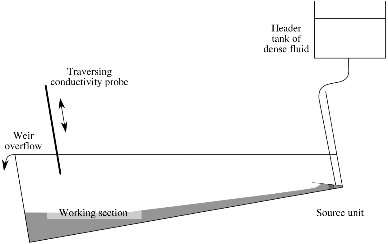
The experiments were carried out in a rectangular tank 2.35 m in length, 0.15 m in width and 0.5 m in height. The tank was inclined at an angle of
 $8.6^{\circ }$
. The apparatus, shown in figure 1, is described in more detail in Hogg et al. (Reference Hogg, Dalziel, Huppert and Imberger2015). The region with triangular vertical cross-section, located below the height of the source formed the working section of the experiments, shown in the photographs in figure 2. The end of the tank formed a weir. The outlet over the weir maintained a constant depth in the basin and was far from the part of the basin where the filling box flow occurred. The basin was initially filled with fresh water. A source unit delivered salt water (aqueous sodium chloride solution) with a reduced gravity of
 $g_{s}^{\prime }=0.20~\text{m}~\text{s}^{-2}$
at a volume flux that remained constant during each run, where
 $g_{s}^{\prime }=g(\unicode[STIX]{x1D70C}_{s}-\unicode[STIX]{x1D70C}_{a})/\unicode[STIX]{x1D70C}_{r}$
,
 $g$
is the acceleration due to gravity,
 $\unicode[STIX]{x1D70C}_{s}$
is the density of the source fluid,
 $\unicode[STIX]{x1D70C}_{a}$
the density of the ambient fluid and
 $\unicode[STIX]{x1D70C}_{r}$
a constant reference density of 1000
 $\text{kg}~\text{m}^{-3}$
. The incoming saltwater propagated as a gravity current along the slope, accumulating in a ponded region at the bottom of the basin.
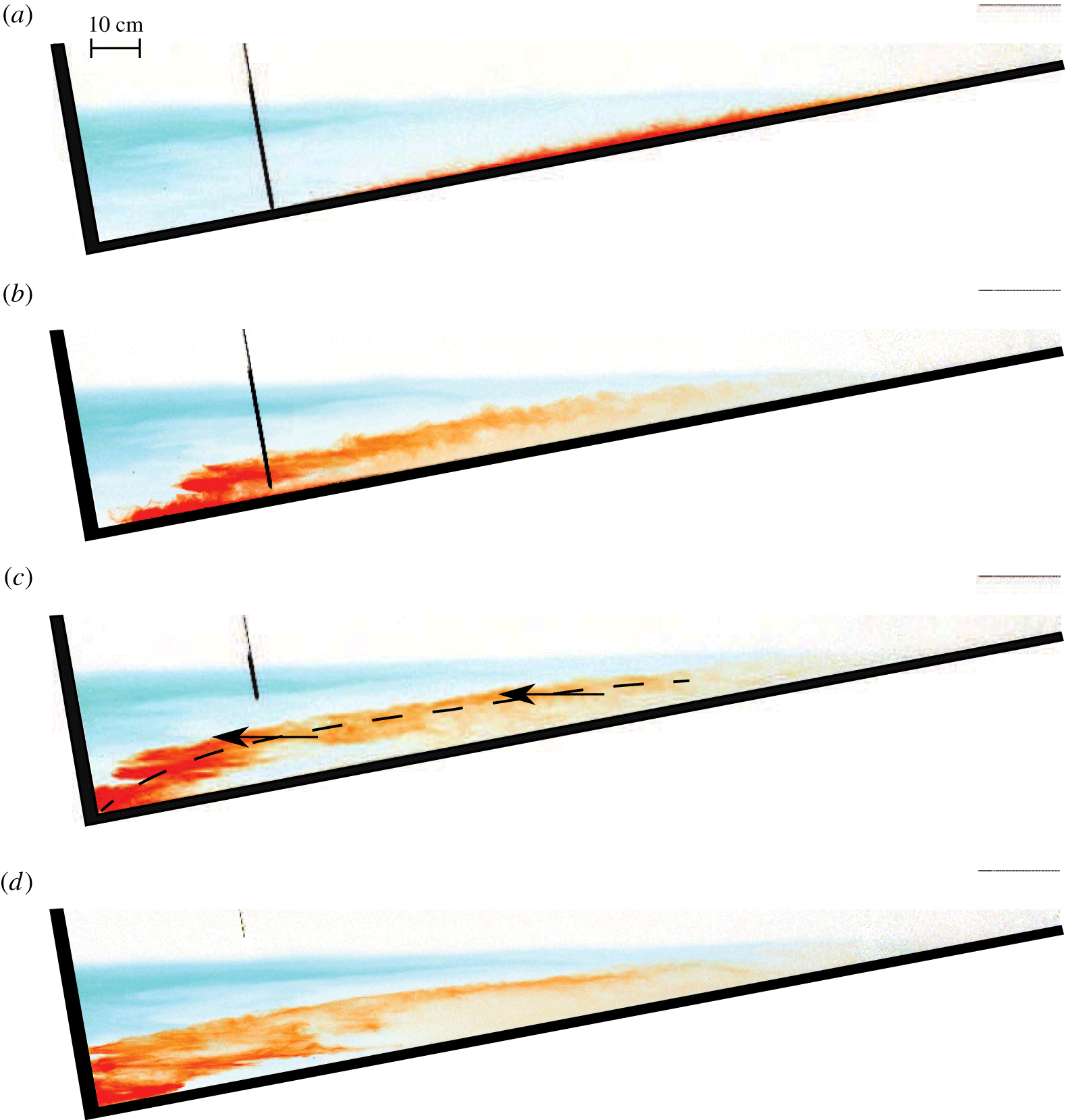
Qualitative observations of the transport pathway of the inflowing fluid through the basin were made by adding pulses of different coloured dyes to the continuously flowing source. The dye was pre-diluted with source fluid to ensure that it had the same density as the source fluid. Each pulse of dye was injected rapidly, over less than 1 s. The tank was illuminated from behind with a diffuse light bank and photographed at two second intervals with a colour digital camera. The intensity measured for each colour channel in the images was divided by the intensity in the initial image, in which no dye was present, to remove the background image. In the qualitative experiments, the source solution had a reduced gravity of
 $0.60~\text{m}~\text{s}^{-2}$
relative to the initial tank fluid. The dye visualisation at a source flow rate per unit width of
 $6.1\times 10^{-4}~\text{m}^{2}~\text{s}^{-1}$
is shown in figure 2. The source Reynolds number,
 $Re_{s}=Q_{s}/\unicode[STIX]{x1D708}$
, was 600, where
 $Q_{s}$
is the source volume flux per unit width and
 $\unicode[STIX]{x1D708}$
the kinematic viscosity. The value of
 $\unicode[STIX]{x1D708}$
was constant throughout these experiments, meaning that
 $Re_{s}$
was a function of
 $Q_{s}$
alone.
For the quantitative experiments, runs were conducted at 10 different values of
 $Q_{s}$
. The full density profile in the basin was measured every 13 s with an aspirating conductivity probe located 35 cm from the end wall, which moved downwards on a traverse at
 $50~\text{mm}~\text{s}^{-1}$
whilst taking samples at 0.5 mm intervals. The probe gave errors in the density measurements with a standard deviation of
 $0.8~\text{kg}~\text{m}^{-3}$
during calibration, or 4 % of the reduced gravity of the source fluid. The density profiles were filtered with a 3 mm moving average filter. Scales smaller than this were influenced by electrical noise in the conductivity probe and were unimportant to the large scale stratification considered in this article.
Schematic of the laboratory apparatus.

Images showing the evolution of a pulse of red dye injected into a continuous-flux gravity current. These images are from the supplementary movie. The dense fluid is supplied at the top of the slope, at the right-hand edge of the image, and immediately moves downslope. The images were taken at 10 s intervals, with (a) at
 $t=90$
s. The red dye was introduced at
 $t=80$
s. The dashed line in (c) indicates the location of the pulse of red dye in the outer layer of the gravity current and the arrows indicate its motion into the ambient fluid. The traversing probe is visible towards the left of the tank.

3 Results
3.1 Qualitative results
Photographs during the run at
 $Re_{s}=600$
are shown in figure 2 at 10 s intervals, starting at 90 s after the source was initiated. The path of the red dye during this part of the filling process shows the peeling detrainment that is the focus of this article. A movie of the full duration of the basin filling is available in the supplementary movie at https://doi.org/10.1017/jfm.2017.196, which shows the motion more clearly than the still photographs. The first pulse of dye, which was blue, was added to the gravity current as the source was turned on, at time
 $t=0$
s. As shown in the movie, the head of the gravity current travelled down the slope. As the dyed fluid propagated down the slope, the current was diluted with ambient fluid brought into the current by turbulent entrainment. It was visually apparent that the gravity current was turbulent, shown by the wisps and eddies at the edge of the red dye patch in figure 2(a) and, more clearly, from the motion in the accompanying movie. The turbulent nature of the entrainment at the upper edge of the gravity current was shown specifically in figure 3(a) of Hogg et al. (Reference Hogg, Dalziel, Huppert and Imberger2015) by using milk as an opaque dye. Experiments in rotating and non-rotating systems have also found gravity currents at these Reynolds numbers were turbulent (Cenedese et al.
Reference Cenedese, Whitehead, Ascarelli and Ohiwa2004; Cenedese & Adduce Reference Cenedese and Adduce2008). Those studies showed that at Reynolds numbers below approximately 100 the gravity currents were laminar, and had much smaller values of the entrainment coefficient. When the head reached the bottom of the tank (
 $t\approx 20$
s), it crashed against the end wall and established the stratified ponded region. Waves were then reflected back away from the end wall and soon dissipated, leaving a horizontal front. The initial stage of the filling, influenced by the crashing of the gravity current head, is not the focus of this article. As the gravity current delivered more fluid to the ponded region, the front rose. The top of the blue layer in figure 2 indicates the top of the stratified ponded region, with clear fluid of uniform density above it.
The image in figure 2(a) shows the current 10 s after the red pulse was injected into the source. The red dye propagated down along the slope, confined to the gravity current at the boundary. The front of the red dye in the gravity current did not have a head structure because the quasi-steady gravity current was already flowing before the dye was injected.
The part of the dyed current closest to the slope descended to the bottom of the basin. The outer part of the gravity current, further from the slope, did not reach to the bottom of the tank. Instead, as shown in figure 2(b,c), a band of red dye moved out horizontally, directly into the ambient fluid across almost the whole depth of the ponded region. This band of red dye contained fluid that was neutrally buoyant at different heights in the ponded region. The red fluid ranged from being marginally denser than the initial basin fluid, near the top of the ponded region, to being the densest fluid in the ponded region, at the bottom of the ponded region. This was shown by the density profiles, which will be discussed in § 3.2. No red dye entered the part of the ambient fluid with uniform density above the ponded region.
Between dye pulses, the source was supplied with the same volume flux and buoyancy flux, but with undyed, clear fluid. In figure 2(c), the region along the boundary beneath the red dye was not dyed red because the current had been refreshed with undyed source fluid carried by the gravity current. In this region, dilute blue fluid was present, showing that the gravity current continued to entrain blue fluid from the ponded region as it descended.
Within the stratified part of the ambient fluid, a complex field of internal waves was visible from the motion of the dye. The motion of the dye suggested that in the stratified part of the ambient fluid mixing was weaker during this part of the experiment. In addition, the Thorpe scale calculated from the conductivity probe measurements in the stratified part of the ambient during this later stage of the experiment was less than 0.005 m, an order of magnitude smaller than that measured immediately after the head of the gravity current crashed against the end wall.
Once the red dye pulse moved out into the ambient fluid the internal waves contributed to the transport of the dye throughout the ambient fluid. Shear waves predominantly moved the ambient fluid horizontally. This motion made zigzag patterns in the dye, as shown in figure 2(c,d), reminiscent of the shear waves formed in stratified fluids by withdrawal and injection (Imberger & Fandry Reference Imberger and Fandry1975). We conjecture that the shear waves in the stratified part of the ambient fluid are energised by the gravity current entering the stratified fluid, as found by Wong et al. (Reference Wong, Griffiths and Hughes2001) for a vertically falling plume. A detailed study of these internal waves would be valuable, but is not the focus of this work. A pulse of green dye, added later during the experiment, behaved similarly to the red dye pulse, as can be seen in the supplementary movie.
At other flow rates, and corresponding
 $Re_{s}$
, a similar peeling detrainment behaviour was observed. In all runs, the dye pulse moved away from the boundary into the ambient fluid directly across a range of depths in the stratified ponded region, rather than upwelling from the bottom of the ponded region. The flow entering the ambient fluid had substantially different characteristics depending on
 $Re_{s}$
and how energetic the eddies in the gravity current were. At
 $Re_{s}=100$
, the dye pulse moved into the ponded region as a thin band with little turbulent dispersion. At this
 $Re_{s}$
, the run was in the regime in which the gravity current appeared laminar when descending through the uniform upper layer of the ambient, as discussed in Hogg et al. (Reference Hogg, Dalziel, Huppert and Imberger2015). At
 $Re_{s}=870$
the dye pulse moved into the ambient fluid as a wide and diffuse cloud. At this
 $Re_{s}$
the run was in the regime in which the gravity current appeared turbulent when descending through the uniform upper layer of the ambient (Hogg et al.
Reference Hogg, Dalziel, Huppert and Imberger2015).
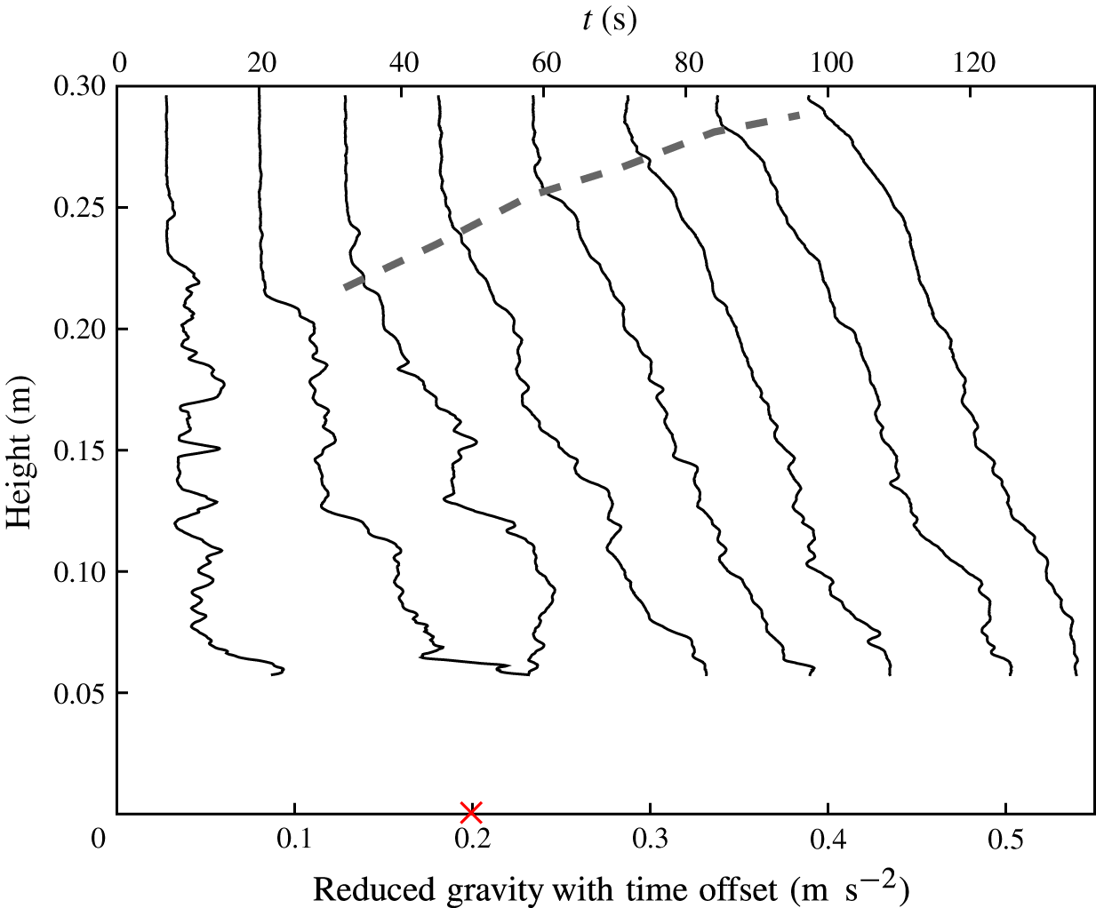
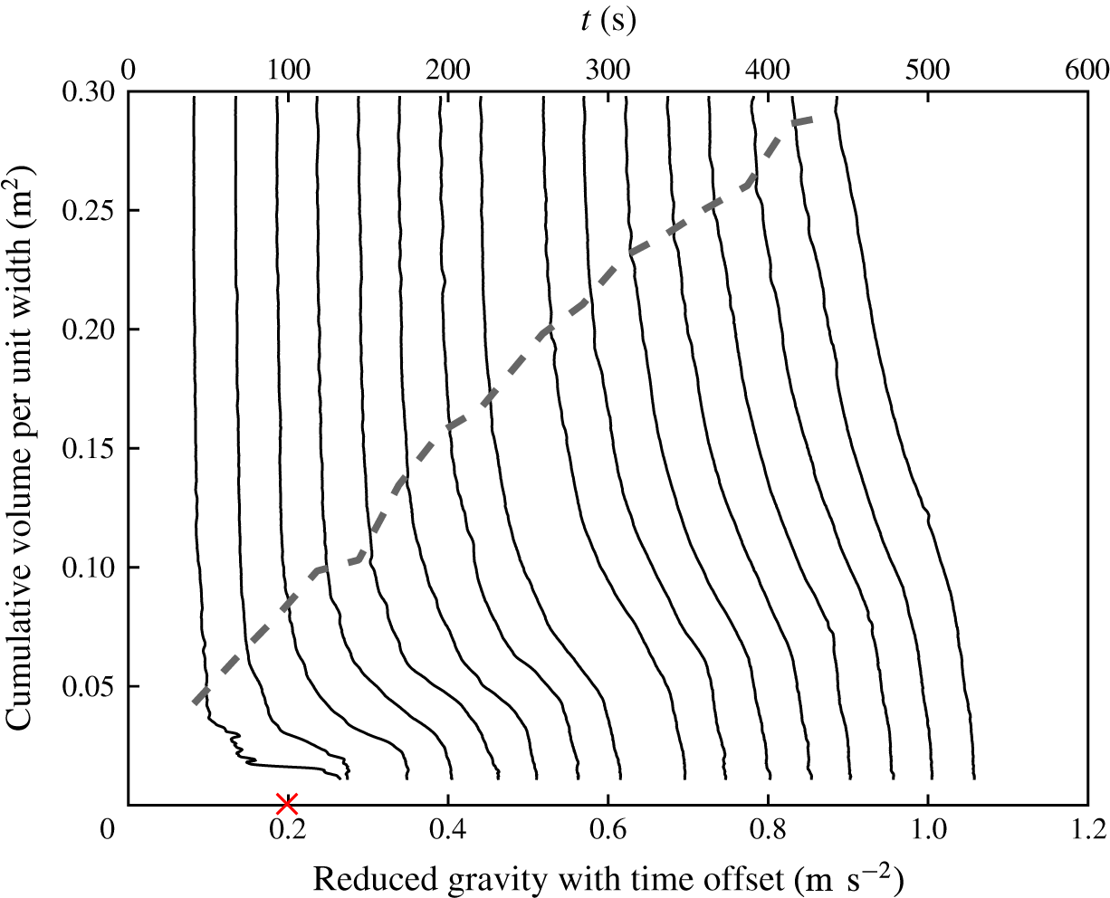
Profiles of reduced gravity measured in an experiment with
 $Re_{s}=990$
. Each profile is offset by the time at which that profile measurement began, such that
 $g^{\prime }+t/250$
is plotted on the abscissa. The thick grey dashed line shows the rising front of the ponded region. Height is measured vertically above the deepest point in the basin. The reduced gravity of the source is indicated with no time offset by the red cross on the abscissa.

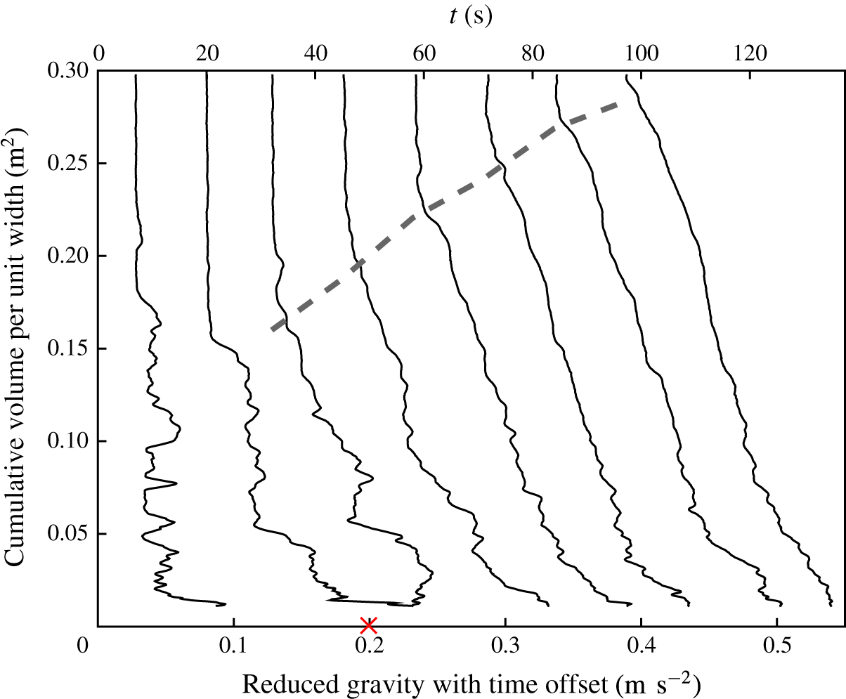
Profiles of reduced gravity from figure 3, plotted with cumulative volume from the bottom of the tank on the
 $y$
-axis. The grey dashed line shows the rising front of the ponded region. The reduced gravity of the source is indicated with no time offset by the red cross.

3.2 Quantitative results
The density measurements confirm that dense fluid accumulated in the ponded region, as seen in the dye visualisation experiments. Figure 3 shows the density profiles plotted against height for the experiment with
 $Re_{s}=990$
. The rising front of the ponded region is indicated by the thick, grey, dashed line. The front was identified in each profile as the height at which the density difference fell below 10 % of that at the source. These observed frontal rise curves compared well with the modelled upwelling velocity, as shown in figure 9 of Hogg et al. (Reference Hogg, Dalziel, Huppert and Imberger2015).
Plotting the density profiles against depth gives undue emphasis to small volumes of fluid towards the bottom vertex of the tank, where the horizontal cross-sectional area vanishes. Throughout the rest of this article, the density profiles will be plotted against the cumulative volume from the bottom of the triangular tank. For comparison with figure 3, the same density profiles are plotted against cumulative volume in figure 4.
The profiles contain regions of static instability, shown by the non-monotonic reduction in density with height, within an overall stable profile. The statically unstable parts of the density profiles were produced by eddies raising dense fluid as they overturned. The departures from monotonicity are largest in the earliest profiles shortly after the gravity current head hit the wall, when turbulent overturns were still occurring. As well as being statically unstable in places, the early density profiles established by the crashing of the head of the current had sharp density discontinuities. As the basin filled, the density discontinuities in the profiles became smoother. In the less energetic runs at lower
 $Re_{s}$
, such as that shown in figure 5, there were fewer inversions and discontinuities in the early density profiles.
Profiles measured in an experiment with
 $Re_{s}=370$
. The reduced gravity is offset by the time at which the profile was taken, such that
 $g^{\prime }+t/500$
is plotted on the abscissa. For clarity, only every other profile is plotted. The grey dashed line shows the rising front of the ponded region. The reduced gravity of the source is indicated with no time offset by the red cross.

The density of fluid at the bottom of the profiles gradually increased over the course of the experiment towards the density of the source. This increase occurred because, as the basin filled with more dense fluid, the gravity current mixed with denser fluid during its descent. This process is similar to that of the classical Baines & Turner (Reference Baines and Turner1969) model.
4 Theoretical models
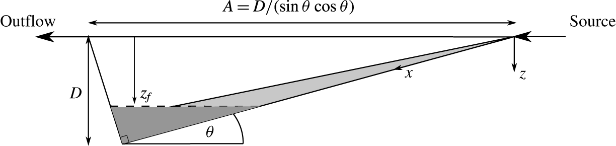
We shall compare our observations with two models of how the boundary current fluid exchanged with the ambient fluid: the prevailing model originally discussed by Baines & Turner (Reference Baines and Turner1969), which we call the ‘persistently entraining gravity current model’; and an extension of the model to include peeling detrainment, which we call the ‘peeling gravity current model’. A schematic of the models is given in figure 6.
In both these models, the entrainment into the gravity current in the uniform density part of the ambient fluid is described by the entrainment hypothesis (Turner Reference Turner1986). This hypothesis states that the entrainment velocity with which fluid is drawn into the gravity current is linearly proportional to the characteristic velocity of the gravity current. The coefficient of proportionality is termed the entrainment coefficient,
 $E$
. The models differ in what happens within the stratified ponded region. A theory for detrainment from a gravity current in a stratified ambient fluid was developed by Baines (Reference Baines2001). We have not used this more complicated theory here because it used experimentally measured parameters, such as drag coefficients, that we were not able to determine.
Schematic of the basin used in the models. The gravity current is shown in light grey and the ponded region is shown in dark grey. The displacements
 $z$
and
 $x$
describe the vertical and downslope displacement below the virtual origin of the source. The depth of the tank below the virtual origin is
 $D$
,
 $A$
is the horizontal length of the basin at the height of the virtual origin and
 $z_{f}$
is the depth of the front of the ponded region below the virtual origin.

4.1 Persistently entraining gravity current model
In the persistently entraining model (Baines & Turner Reference Baines and Turner1969), the gravity current entrains fluid along its whole length, according to the entrainment hypothesis. Entrainment occurs both in the uniform and the stratified parts of the ambient fluid. In this model, outflow of fluid from along the length of the current into the stratified ambient fluid does not occur. The circulation implied by the persistently entraining model is that all gravity current fluid falls to the bottom of the basin and then rises in the ambient fluid (Baines & Turner Reference Baines and Turner1969).
The fluxes in the gravity current are calculated from conservation equations, under the Boussinesq approximation. Conservation of volume, momentum, and buoyancy imply
 $$\begin{eqnarray}\displaystyle & \displaystyle \frac{\text{d}}{\text{d}x}(uh)=Eu, & \displaystyle\end{eqnarray}$$
 $$\begin{eqnarray}\displaystyle & \displaystyle \unicode[STIX]{x1D70C}_{r}\frac{\text{d}}{\text{d}x}(u^{2}h)=\unicode[STIX]{x1D70C}_{r}g^{\prime }h\sin \unicode[STIX]{x1D703}, & \displaystyle\end{eqnarray}$$
 $$\begin{eqnarray}\displaystyle & \displaystyle \frac{\text{d}}{\text{d}x}(uhg^{\prime })=-uh\frac{\text{d}}{\text{d}x}g_{a}^{\prime }, & \displaystyle\end{eqnarray}$$
respectively. Here,
 $x$
is the distance along the slope from the source,
 $u$
the depth-averaged velocity down the slope in the gravity current,
 $h$
the thickness of the gravity current normal to the slope,
 $E$
the entrainment coefficient,
 $g^{\prime }=g(\unicode[STIX]{x1D70C}_{p}-\unicode[STIX]{x1D70C}_{a})/\unicode[STIX]{x1D70C}_{r}$
the depth-averaged reduced gravity of the fluid in the current,
 $g_{a}^{\prime }=g(\unicode[STIX]{x1D70C}_{a}-\unicode[STIX]{x1D70C}_{r})/\unicode[STIX]{x1D70C}_{r}$
the reduced gravity of the ambient fluid,
 $\unicode[STIX]{x1D703}$
the angle the incline makes with horizontal and
 $\unicode[STIX]{x1D70C}_{p}$
the density averaged across the thickness of the gravity current. The values of
 $E$
were found from a linear parameterisation for
 $E(Re_{s})$
determined from the rise of the front of the ponded region, as described in Hogg et al. (Reference Hogg, Dalziel, Huppert and Imberger2015). The incline of the slope in our experiments was steep enough that drag was small relative to the gravitational acceleration along the slope. Drag was therefore neglected from (4.2).
In this model, as is common in the literature, the ensemble-averaged density and velocity profiles are assumed to have a ‘top-hat’ form (Morton et al.
Reference Morton, Taylor and Turner1956), described by a Heaviside step function falling to the ambient value at a distance
 $h$
perpendicular to the slope. The persistently entraining model described by Baines & Turner (Reference Baines and Turner1969) implies a uniform, top-hat density profile within the gravity current. In their model, all fluid discharged from the gravity current at any instant has the same neutral buoyancy depth and therefore the same density.
The ambient density stratification in the basin is modified because fluid is withdrawn by entrainment from the ambient fluid and dense fluid is discharged into the bottom of the basin by the gravity current. The evolution of the ambient density profile is set by the upwelling advection of the ambient fluid, which balances the downwards volume flux in the gravity current. For the triangular basin used in these experiments the Baines & Turner (Reference Baines and Turner1969) model was adapted, such that the density evolution is
 $$\begin{eqnarray}\frac{\unicode[STIX]{x2202}g_{a}^{\prime }}{\unicode[STIX]{x2202}t}=\frac{uh}{A}\frac{\unicode[STIX]{x2202}g_{a}^{\prime }}{\unicode[STIX]{x2202}z},\end{eqnarray}$$
where
 $A=(D-z)/(\sin \unicode[STIX]{x1D703}\cos \unicode[STIX]{x1D703})$
is the horizontal length of the basin,
 $D$
is the depth of the basin below the virtual origin and
 $z=x\sin \unicode[STIX]{x1D703}$
is the vertical distance beneath the virtual origin. The virtual origin is the location, offset above the physical source, at which a source of buoyancy alone would give rise to the volume and buoyancy fluxes that occurs at the physical source (Hunt & Kaye Reference Hunt and Kaye2001). Fluid is assumed to pass through the gravity current instantaneously relative to the time scale of changes in the basin stratification.
The variables in (4.1)–(4.4) can be made dimensionless with the scalings
 $$\begin{eqnarray}\displaystyle & \displaystyle \unicode[STIX]{x1D701}=1-\unicode[STIX]{x1D702}=zD^{-1}, & \displaystyle\end{eqnarray}$$
 $$\begin{eqnarray}\displaystyle & \displaystyle \unicode[STIX]{x1D70F}=tE^{2/3}{F_{0}}^{1/3}\sin ^{1/3}\unicode[STIX]{x1D703}\cos \unicode[STIX]{x1D703}D^{-1}, & \displaystyle\end{eqnarray}$$
 $$\begin{eqnarray}\displaystyle & \displaystyle f=g^{\prime }uhF_{0}^{-1}, & \displaystyle\end{eqnarray}$$
 $$\begin{eqnarray}\displaystyle & \displaystyle q=uh\sin ^{2/3}\unicode[STIX]{x1D703}E^{-2/3}D^{-1}F_{0}^{-1/3}, & \displaystyle\end{eqnarray}$$
 $$\begin{eqnarray}\displaystyle & \displaystyle m=u^{2}h\sin ^{1/3}\unicode[STIX]{x1D703}E^{-1/3}D^{-1}F_{0}^{-2/3}, & \displaystyle\end{eqnarray}$$
 $$\begin{eqnarray}\displaystyle & \displaystyle \unicode[STIX]{x1D6FF}=g_{a}^{\prime }E^{2/3}D\sin ^{-2/3}\unicode[STIX]{x1D703}F_{0}^{-2/3}, & \displaystyle\end{eqnarray}$$
where
 $\unicode[STIX]{x1D701}$
is the dimensionless distance below the virtual origin,
 $\unicode[STIX]{x1D702}$
the dimensionless distance above the bottom of the tank,
 $\unicode[STIX]{x1D70F}$
the dimensionless time since the source began,
 $f$
the dimensionless buoyancy flux per unit width,
 $q$
the dimensionless volume flux per unit width,
 $m$
the dimensionless momentum flux per unit width,
 $\unicode[STIX]{x1D6FF}$
the dimensionless reduced gravity and
 $F_{0}$
the source buoyancy flux per unit width. This gives the dimensionless form of (4.1)–(4.4) as
 $$\begin{eqnarray}\displaystyle & \displaystyle \frac{\text{d}q}{\text{d}\unicode[STIX]{x1D701}}=\frac{m}{q}, & \displaystyle\end{eqnarray}$$
 $$\begin{eqnarray}\displaystyle & \displaystyle \frac{\text{d}m}{\text{d}\unicode[STIX]{x1D701}}=\frac{fq}{m}, & \displaystyle\end{eqnarray}$$
 $$\begin{eqnarray}\displaystyle & \displaystyle \frac{\text{d}f}{\text{d}\unicode[STIX]{x1D701}}=-q\frac{\text{d}\unicode[STIX]{x1D6FF}}{\text{d}\unicode[STIX]{x1D701}}, & \displaystyle\end{eqnarray}$$
 $$\begin{eqnarray}\displaystyle & \displaystyle \frac{\unicode[STIX]{x2202}\unicode[STIX]{x1D6FF}}{\unicode[STIX]{x2202}\unicode[STIX]{x1D70F}}=\frac{q}{1-\unicode[STIX]{x1D701}}\frac{\unicode[STIX]{x2202}\unicode[STIX]{x1D6FF}}{\unicode[STIX]{x2202}\unicode[STIX]{x1D701}}. & \displaystyle\end{eqnarray}$$
The initial condition for the filling process is
 $\unicode[STIX]{x1D6FF}(\unicode[STIX]{x1D70F}=0,\unicode[STIX]{x1D701})=0$
, and the boundary conditions at the virtual origin are
 $f(0)=1$
,
 $q(0)=0$
and
 $m(0)=0$
. The density of fluid that enters at the bottom of the basin is set by the density of fluid in the gravity current when it reaches the bottom of the current.
The system of equations (4.11)–(4.14) was solved numerically using the scheme from Germeles (Reference Germeles1975), adapted for a triangular basin, which we will outline. The scheme used the analytic solutions for the gravity current fluxes through the uniform part of the ambient fluid, which are
 $q=\unicode[STIX]{x1D701}$
,
 $m=\unicode[STIX]{x1D701}$
and
 $f=1$
. The gravity current fluxes through the stratified part of the ambient fluid were calculated with (4.11)–(4.13), using a second-order Runge–Kutta scheme for the spatial derivatives. The evolution of the isopycnal layers in the ambient stratification was solved by time stepping (4.14) using an Euler integration scheme, with a Lagrangian coordinate system that moves with isopycnal surfaces in the ambient fluid. In this scheme, a layer of dense fluid is deposited by the gravity current at the bottom of the basin at each time step. The layers rise over the following time steps by displacements
 $\unicode[STIX]{x0394}\unicode[STIX]{x1D701}_{i}$
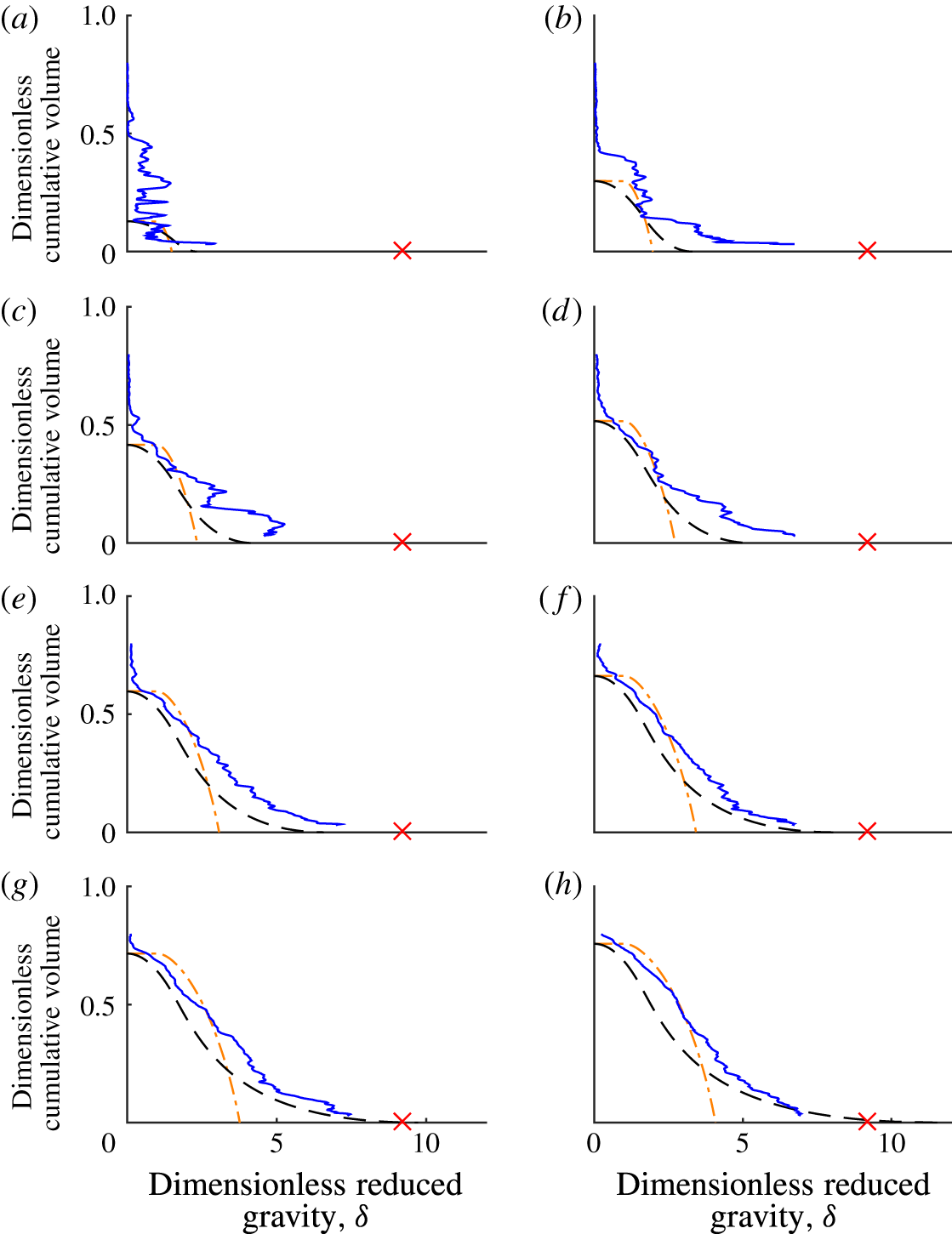
, calculated from (4.14). The scheme was validated by comparison with asymptotic solutions we derived for the gravity current fluxes and ambient profile at large times, reported in Hogg (Reference Hogg2014). The numerical solution for the persistently entraining model is plotted as dot-dashed lines, alongside the experimental measurements and the peeling model solution, in figure 7.
A time series of experimentally observed reduced gravity profiles (blue solid line) plotted using the cumulative volume in the tank on the
 $y$
-axis, with
 $\unicode[STIX]{x1D70F}$
of (a) 0.085, (b) 0.24, (c) 0.39, (d) 0.55, (e) 0.71, (f) 0.87, (g) 1.00 and (h) 1.20. The result of the persistently entraining model (orange dot-dashed line) and the peeling model (black dashed line) are plotted with the observations. The source flow gave
 $Re_{s}=990$
. The reduced gravity of the source is indicated by the red cross.

4.2 Peeling gravity current model
The qualitative observations showed that in the stratified portion of the ambient fluid, namely the ponded region, peeling detrainment transported fluid directly from the gravity current into the ambient fluid over a range of depths. Peeling detrainment was dominant in the ponded region, although we believe that some entrainment continued. This section describes how the behaviour of the persistently entraining model was modified to incorporate a simple model of the observed detrainment transport.
The overall scheme of the peeling model is as follows. When the gravity current travels through the uniform density part of the ambient fluid above the ponded region, entrainment brings ambient fluid into the current. The current and all the fluid entrained into it propagates down the slope until it enters the ponded region. Once the gravity current enters the stratified ponded region, entrainment ceases and peeling detrainment transports fluid from the gravity current into the stratified ambient fluid. By peeling detrainment, we mean that the outer layers of the gravity current peel away from the current and move to their respective neutral buoyancy height in the stratified ambient fluid. We make the simplifying assumption that during the peeling detrainment process in the ponded region, no mixing occurs and the density of the fluid does not change. The peeling detrainment is therefore equivalent to an adiabatic reordering of the fluid delivered by the gravity current to the ponded region.
In the uniform ambient fluid, the gravity current behaves identically to the persistently entraining model. Equations (4.11)–(4.13) apply, and the front of the ponded region rises at the same rate, defined by
 $$\begin{eqnarray}\unicode[STIX]{x1D70F}=\unicode[STIX]{x1D701}_{f}-\ln (\unicode[STIX]{x1D701}_{f})-1,\end{eqnarray}$$
or, when inverted,
 $$\begin{eqnarray}\unicode[STIX]{x1D701}_{f}=-{\mathcal{W}}(-\text{e}^{-1-\unicode[STIX]{x1D70F}}),\end{eqnarray}$$
where
 ${\mathcal{W}}$
is the Lambert-W function (Corless et al.
Reference Corless, Gonnet, Hare, Jeffrey and Knuth1996), also known as the product-log function, and
 $\unicode[STIX]{x1D701}_{f}$
the depth of the front of the ponded region (Hogg et al.
Reference Hogg, Dalziel, Huppert and Imberger2015).
The density profile in the gravity current must be modelled as non-uniform and continuous with the ambient stratification for the observed peeling detrainment to be possible in the stratified ponded region. This is necessary so that fluid in the gravity current can be neutrally buoyant over a continuous range of depths in the stratified ambient fluid. In the present model, the gravity current is assumed to have linear profiles of velocity and density. Such profiles can be viewed as representing the first two terms of the Taylor series approximation to profiles such as those observed by Ellison & Turner (Reference Ellison and Turner1959) and Odier, Chen & Ecke (Reference Odier, Chen and Ecke2014). The profiles of velocity and density at a depth
 $z$
in the basin are, respectively,
 $$\begin{eqnarray}\displaystyle & \displaystyle U=\left\{\begin{array}{@{}ll@{}}\displaystyle U_{m}(H-Y)/H,\quad & Y<H\\ \displaystyle 0,\quad & Y>H,\\ \quad \end{array}\right. & \displaystyle\end{eqnarray}$$
 $$\begin{eqnarray}\displaystyle & \displaystyle \unicode[STIX]{x1D70C}=\left\{\begin{array}{@{}ll@{}}\displaystyle \unicode[STIX]{x1D70C}_{a}+\unicode[STIX]{x1D70C}_{m}(H-Y)/H,\quad & Y<H\\ \displaystyle 0,\quad & Y>H,\end{array}\right. & \displaystyle\end{eqnarray}$$
where
 $U_{m}(z)$
is the maximum velocity in the profile,
 $H(z)$
the thickness of the current,
 $Y$
the perpendicular distance from the slope and
 $\unicode[STIX]{x1D70C}_{m}(z)$
the maximum density difference in the profile relative to the ambient fluid. Linear profiles within gravity currents such as these have been used in other models (e.g. Cooper & Hunt Reference Cooper and Hunt2010) and have been observed in laboratory studies (Ellison & Turner Reference Ellison and Turner1959; Odier et al.
Reference Odier, Chen and Ecke2014). The simple profile functions chosen here are sufficient to demonstrate the impact of peeling detrainment on the stratification in the filling basin, although we note that peeling detrainment mechanisms are not limited to the case of linear profiles.
The fluxes of volume, momentum and buoyancy in currents with the linear profiles (4.17) and (4.18) are, respectively,
 $$\begin{eqnarray}\displaystyle & \displaystyle Q=\int _{0}^{H}U\,\text{d}Y=\frac{U_{m}H}{2}, & \displaystyle\end{eqnarray}$$
 $$\begin{eqnarray}\displaystyle & \displaystyle M=\unicode[STIX]{x1D70C}_{r}\int _{0}^{H}U^{2}\,\text{d}Y=\frac{\unicode[STIX]{x1D70C}_{r}U_{m}^{2}H}{3}, & \displaystyle\end{eqnarray}$$
 $$\begin{eqnarray}\displaystyle & \displaystyle F=\int _{0}^{H}\frac{g}{\unicode[STIX]{x1D70C}_{r}}(\unicode[STIX]{x1D70C}-\unicode[STIX]{x1D70C}_{a})U\,\text{d}Y=\frac{G_{m}^{\prime }U_{m}H}{3}, & \displaystyle\end{eqnarray}$$
where
 $G_{m}^{\prime }=g(\unicode[STIX]{x1D70C}_{m}-\unicode[STIX]{x1D70C}_{a})/\unicode[STIX]{x1D70C}_{r}$
is the maximum reduced gravity in the current relative to the local ambient fluid. Here the fluxes are defined in terms of the maximum values
 $G_{m}^{\prime }$
and
 $U_{m}$
, rather than the average values
 $g^{\prime }$
and
 $u$
used in (4.1)–(4.3).
Because the current velocity profile is linear in the peeling model, the value of the entrainment coefficient is different from that for the top-hat profile used in the persistently entraining model, analogous to the difference between Gaussian and top-hat plume profiles. To allow the two models to be compared, we here define the equivalent entrainment coefficient for the linear case as
 $E_{eq}=3W/(2U_{m})$
. Using
 $E_{eq}$
, the evolution of the volume and momentum flux of the gravity current in the uniform ambient fluid is identical for the two models.
The dimensionless parameters describing the current and the basin, restated in terms of the profile maximum values rather than the mean values used in (4.7)–(4.9), are
 $$\begin{eqnarray}\displaystyle & \displaystyle \unicode[STIX]{x1D70F}=tE_{eq}^{2/3}F_{0}^{1/3}\sin ^{1/3}\unicode[STIX]{x1D703}\cos \unicode[STIX]{x1D703}D^{-1}, & \displaystyle\end{eqnarray}$$
 $$\begin{eqnarray}\displaystyle & \displaystyle f=\frac{G_{m}^{\prime }U_{m}H}{3}F_{0}^{-1}, & \displaystyle\end{eqnarray}$$
 $$\begin{eqnarray}\displaystyle & \displaystyle q=\frac{U_{m}H}{2}\sin ^{2/3}\unicode[STIX]{x1D703}E_{eq}^{-2/3}D^{-1}F_{0}^{-1/3}, & \displaystyle\end{eqnarray}$$
 $$\begin{eqnarray}\displaystyle & \displaystyle m=\frac{U_{m}^{2}H}{3}\sin ^{1/3}\unicode[STIX]{x1D703}E_{eq}^{-1/3}D^{-1}F_{0}^{-2/3}, & \displaystyle\end{eqnarray}$$
 $$\begin{eqnarray}\displaystyle & \displaystyle \unicode[STIX]{x1D6FF}=g_{a}^{\prime }E_{eq}^{2/3}D\sin ^{-2/3}\unicode[STIX]{x1D703}F_{0}^{-2/3}. & \displaystyle\end{eqnarray}$$
These are the appropriate scalings for gravity currents with linear profiles of density and velocity.
Because it is assumed that no mixing occurs in the ponded region, the height,
 $\unicode[STIX]{x1D702}_{i}$
, of an isopycnal with reduced gravity
 $\unicode[STIX]{x1D6FF}_{i}$
at time
 $\unicode[STIX]{x1D70F}$
can be calculated by integrating the volume flux of fluid delivered to the ponded region with density greater than
 $\unicode[STIX]{x1D6FF}_{i}$
. This height is
 $$\begin{eqnarray}\unicode[STIX]{x1D702}_{i}(\unicode[STIX]{x1D6FF}_{i},\unicode[STIX]{x1D70F})=\sqrt{2\int _{\unicode[STIX]{x1D70F}_{i}}^{\unicode[STIX]{x1D70F}}q_{i}\,\text{d}\unicode[STIX]{x1D70F}},\end{eqnarray}$$
where
 $q_{i}$
is the volume flux in the current with density greater than
 $\unicode[STIX]{x1D6FF}_{i}$
, and
 $\unicode[STIX]{x1D70F}_{i}$
the time at which fluid of density
 $\unicode[STIX]{x1D6FF}_{i}$
first reaches the ponded region. We must calculate the volume flux in the gravity current after it has travelled through the uniform density ambient fluid, just before entering the ponded region. The profiles in the current, equations (4.17) and (4.18), give this volume flux as
 $$\begin{eqnarray}q_{i}(\unicode[STIX]{x1D6FF}_{i},\unicode[STIX]{x1D701})=\int _{0}^{y_{i}}u_{m}(1-y/h)\,\text{d}y,\end{eqnarray}$$
where
 $u_{m}=2q/h$
is the dimensionless maximum velocity in the current at
 $\unicode[STIX]{x1D701}$
,
 $y_{i}=h[1-(\unicode[STIX]{x1D6FF}_{i}/\unicode[STIX]{x1D6FF}_{m})]$
is the dimensionless thickness of the part of the current with density greater than
 $\unicode[STIX]{x1D6FF}_{i}$
,
 $h(\unicode[STIX]{x1D701})$
is the dimensionless thickness of the current and
 $\unicode[STIX]{x1D6FF}_{m}(\unicode[STIX]{x1D701})=3f/(2q)$
is the dimensionless maximum density in the current. In these expressions, we use the solution
 $h=\unicode[STIX]{x1D701}$
,
 $f=1$
and
 $q=\unicode[STIX]{x1D701}$
to the system of equations (4.11)–(4.13) describing the gravity current in the uniform part of the ambient fluid.
The time
 $\unicode[STIX]{x1D70F}_{i}$
, at which fluid of density
 $\unicode[STIX]{x1D6FF}_{i}$
first reaches the ponded region, can be evaluated by noting that the gravity current fluid is diluted with ambient fluid as it runs down the slope, such that
 $\unicode[STIX]{x1D6FF}_{m}=3/(2\unicode[STIX]{x1D701})$
. Fluid of density
 $\unicode[STIX]{x1D6FF}_{i}$
only starts to enter the ponded region once the ponded region has reached the height at which
 $\unicode[STIX]{x1D6FF}_{m}(\unicode[STIX]{x1D701})=\unicode[STIX]{x1D6FF}_{i}$
. Fluid with
 $\unicode[STIX]{x1D6FF}_{i}<3/2$
enters the ponded region from the beginning of the filling process, at
 $\unicode[STIX]{x1D70F}=0$
. Fluid with
 $\unicode[STIX]{x1D6FF}_{i}>3/2$
, starts to reach the ponded region when
 $\unicode[STIX]{x1D701}_{f}=3/(2\unicode[STIX]{x1D6FF}_{i})$
, which, from (4.15), occurs at
 $$\begin{eqnarray}\unicode[STIX]{x1D70F}_{i}=\left\{\begin{array}{@{}ll@{}}\displaystyle 0,\quad & \unicode[STIX]{x1D6FF}<3/2\\ \displaystyle 3/(2\unicode[STIX]{x1D6FF}_{i})+\ln (2\unicode[STIX]{x1D6FF}_{i}/3)-1,\quad & \unicode[STIX]{x1D6FF}>3/2.\end{array}\right.\end{eqnarray}$$
The evolving stratification may be determined by substituting
 $q_{i}$
and
 $\unicode[STIX]{x1D70F}_{i}$
into (4.27), giving
 $$\begin{eqnarray}\displaystyle \unicode[STIX]{x1D702}_{i} & = & \displaystyle \left\{\begin{array}{@{}ll@{}}\displaystyle \sqrt{2\int _{0}^{\unicode[STIX]{x1D70F}}2\int _{0}^{h(1-2\unicode[STIX]{x1D6FF}_{i}\unicode[STIX]{x1D701}_{f}/3)}\left(1-\frac{y}{h}\right)\,\text{d}y\,\text{d}\unicode[STIX]{x1D70F}},\quad & \unicode[STIX]{x1D6FF}_{i}<3/2\\ \displaystyle \sqrt{2\int _{3/(2\unicode[STIX]{x1D6FF}_{i})-\ln (3/(2\unicode[STIX]{x1D6FF}_{i}))-1}^{\unicode[STIX]{x1D70F}}2\int _{0}^{h(1-2\unicode[STIX]{x1D6FF}_{i}\unicode[STIX]{x1D701}_{f}/3)}\left(1-\frac{y}{h}\right)\,\text{d}y\,\text{d}\unicode[STIX]{x1D70F}},\quad & \unicode[STIX]{x1D6FF}_{i}>3/2\end{array}\right.\nonumber\\ \displaystyle & = & \displaystyle \left\{\begin{array}{@{}ll@{}}\displaystyle \left\{[{\mathcal{W}}(-\text{e}^{-\unicode[STIX]{x1D70F}-1})+1]^{2}-\frac{2}{27}\unicode[STIX]{x1D6FF}_{i}^{2} [\!3{\mathcal{W}}(-\text{e}^{-\unicode[STIX]{x1D70F}-1})^{4}\right.\quad \\ \left.+\,4{\mathcal{W}}(-\text{e}^{-\unicode[STIX]{x1D70F}-1})^{3}+1\!]\right\}^{1/2},\quad & \unicode[STIX]{x1D6FF}_{i}<3/2\\ \left\{\displaystyle \frac{2}{27}\unicode[STIX]{x1D6FF}_{i}^{2}[3C^{4}+4C^{3}-3{\mathcal{W}}(-\text{e}^{\unicode[STIX]{x1D70F}-1})^{4}-4{\mathcal{W}}(-\text{e}^{\unicode[STIX]{x1D70F}-1})^{3}]\right.\quad \\ \left.-\,C^{2}-2C+{\mathcal{W}}(-\text{e}^{\unicode[STIX]{x1D70F}-1})^{2}+2{\mathcal{W}}(-\text{e}^{\unicode[STIX]{x1D70F}-1})\right\}^{1/2},\quad & \unicode[STIX]{x1D6FF}_{i}>3/2,\end{array}\right.\end{eqnarray}$$
where
 $C={\mathcal{W}}(-3\text{e}^{-3/(2\unicode[STIX]{x1D6FF}_{i})}/(2\unicode[STIX]{x1D6FF}_{i}))$
. This expression is plotted with dashed black lines in figures 7 and 8 alongside the experimental observations and the persistently entraining model. The expression for the isopycnal heights in a basin of constant horizontal cross-sectional area can be calculated by a similar method; the constant cross-sectional area case has a simpler and more readily interpretable solution, given in Hogg (Reference Hogg2014), which consists of exponential functions rather than product-log functions.
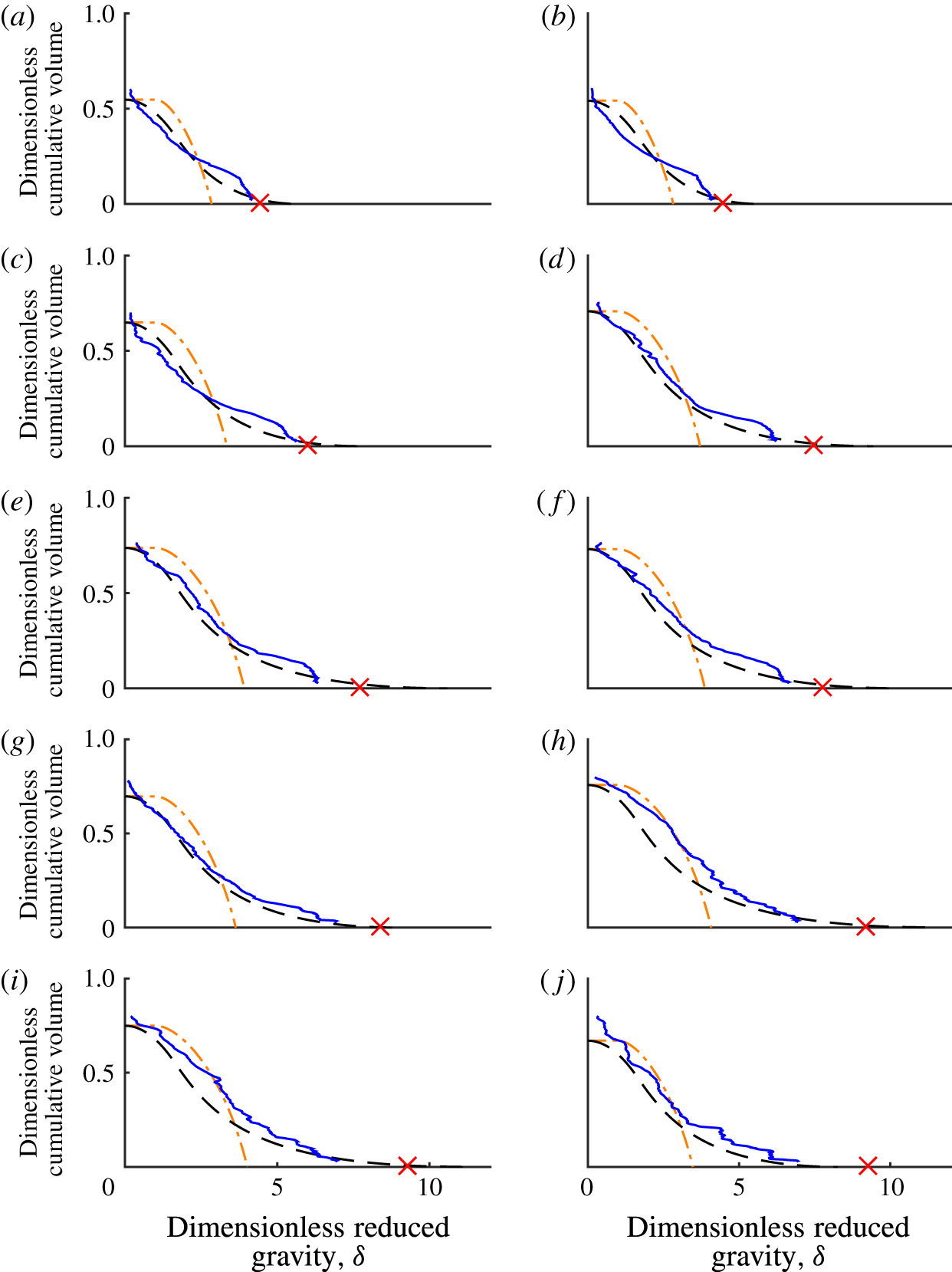
Reduced gravity profile at the time when the ponded region reached the physical source. The profiles are plotted against the cumulative volume in the tank. The measured profile is shown by the blue solid line, the persistently entraining model by the orange dot-dashed line and the peeling model by the black dashed line. All runs in the range
 $350<Re_{s}\leqslant 1100$
are shown, with
 $Re_{s}$
of (a) 360, (b) 370, (c) 440, (d) 580, (e) 620, (f) 630, (g) 730, (h) 990, (i) 1000 and (j) 1100. The reduced gravity of the source is indicated by the red cross.

4.3 Comparison of models with experiments
We will compare the measured density profiles with both the persistently entraining model and the peeling model. The measured profiles were made dimensionless with the scalings (4.5) and (4.6). The results at 8 time steps for the run with
 $Re_{s}=990$
are shown in figure 7 (plotted with solid blue lines). Transport by the quasi-steady gravity current is the focus of this study, not the initial transient of the head. The early density profiles (e.g. for
 $\unicode[STIX]{x1D70F}\lesssim 0.55$
in figure 7) are not well predicted by either model. These early density profiles are influenced by the initial transient of the gravity current head crashing against the end wall, which is not accounted for in the models. Fluid transported by the quasi-steady gravity current is most dominant in the final profiles, shown in figure 8. For each different
 $Re_{s}$
run, the final profile was measured just before the front of the ponded region reached the height of the source unit. The volume of the tank used to normalise the cumulative volume in the plots is the volume below the height of the virtual origin. The distance to the virtual origin reduces as the entrainment coefficient increases, meaning that the distance from the physical source to the virtual origin reduces as
 $Re_{s}$
increases. The height of the virtual origin above the source ranged from 0.09 m for the lowest
 $Re_{s}$
used in these experiments to 0.03 m at higher
 $Re_{s}$
.
The observed density profiles in the high
 $Re_{s}$
run, such as that in figure 7, were closer in form to the peeling model (plotted with black dashed lines) than to the persistently entraining model (plotted with orange dot-dashed lines). This is particularly true at later times, when the continuous gravity current model is appropriate. The observed rates of change of density with cumulative volume are greater than those predicted by the persistently entraining model and are closer to the peeling model. The observed rate of change of density increases towards the bottom of the basin, like the peeling model and in contrast to the persistently entraining model.
The persistently entraining model predicts a discontinuity in the density profile at the front of the ponded region. This occurs because the fluid first deposited by the gravity current into the ponded region, which thereafter remains at the front, has a reduced gravity of
 $\unicode[STIX]{x1D6FF}=1$
, whereas the initial ambient fluid above the front has
 $\unicode[STIX]{x1D6FF}=0$
. The discontinuity predicted by the model can be seen most clearly for runs with low
 $Re_{s}$
, such as at
 $Re_{s}=360$
in figure 8. Such a discontinuity is not predicted by the peeling model, because in this model the density of fluid in the current is continuous with the density of the ambient fluid above the front. Fluid deposited in the ponded region therefore has density ranging continuously from the initial ambient density,
 $\unicode[STIX]{x1D6FF}=0$
, to the peak density in the ponded region. The observed density profiles, like the peeling model, do not exhibit a discontinuity at the front.
The vertical length scale of the profiles, given by the height of the front of the ponded region, is identical in the two models. The vertical length scale is captured well, excepting early times such as
 $\unicode[STIX]{x1D70F}\lesssim 0.55$
in figure 7. The good agreement of the vertical length scale derives from the good agreement between the experiments and the linear fit for
 $E(Re_{s})$
, discussed in Hogg et al. (Reference Hogg, Dalziel, Huppert and Imberger2015).
The density scale of the observations matches the peeling model better than the persistently entraining model, although the density predicted by the peeling model does still deviate somewhat from the observations. For late times in the experiment, for example for
 $\unicode[STIX]{x1D70F}>0.55$
in figure 7, the maximum density predicted by the peeling model is approximately the same as the observations at each time step, with a similar increasing trend. The maximum density predicted by the persistently entraining model has a larger error relative to the observations.
Throughout most runs, the total mass in the basin was slightly underestimated by both models because the models neglected mass introduced into the basin before the transient gravity current reached the bottom of the basin and started to accumulate there, used to define
 $t=0$
in the models. The neglected initial mass addition gave a buoyancy per unit width of up to 0.008
 $\text{m}^{3}~\text{s}^{-2}$
. The deviation in total buoyancy between the model and observations was of a similar magnitude, up to 0.004
 $\text{m}^{3}~\text{s}^{-2}$
. At low source flow rates, corresponding to low
 $Re_{s}$
, both the neglected initial mass addition and the buoyancy deviation between the observations and model reduced. The non-horizontal isopycnals maintained by the gravity current also introduce a source of error in the mass budget.
In the final density profiles, shown in figure 8, the peeling model produced small volumes of fluid with density slightly in excess of the density of the source fluid, which is clearly unphysical behaviour. The unphysically large values of
 $\unicode[STIX]{x1D6FF}$
occur because deviations from the linear parameterisation assumed for
 $E(Re_{s})$
allow the modelled height of the front to reach above the height of the physical source. Closer to the virtual origin than the physical source, the gravity current model has fluid densities greater than the source density. The volume of excessively dense fluid is negligible and is barely visible in the plots.
In experiments with
 $Re_{s}\lesssim 730$
, a relatively homogeneous region was produced over a small volume at the bottom of the basin. As
 $Re_{s}$
reduced, the volume of this homogeneous region increased and the reduced gravity of the fluid increased towards the reduced gravity of the source fluid. At
 $Re_{s}=360$
, fluid close to the source density accumulated at the bottom of the basin from the beginning of the filling process. At the lowest
 $Re_{s}$
shown in figure 8,
 $Re_{s}=360$
, this homogeneous fluid took up 20 % of the tank volume, larger than at any other
 $Re_{s}$
value. At
 $Re_{s}<360$
, the thickness of the homogeneous region grew to take up more of the tank than at
 $Re_{s}=360$
. These low
 $Re_{s}$
runs are not compared to the model here, because the gravity currents in these runs were in a laminar regime where the parameterisation
 $E(Re_{s})$
does not apply (Hogg et al.
Reference Hogg, Dalziel, Huppert and Imberger2015). For low
 $Re_{s}$
runs (e.g.
 $Re_{s}=360$
), some fluid reached the bottom of the basin whilst nearly retaining the source density, suggesting that this undiluted fluid was transported by a somewhat laminar, unmixed sublayer along the base of the gravity current.
The linear profiles (4.18) and (4.17) assumed for the density and velocity profiles do not account for such structure within the gravity current, leading to the discrepancy between the observed ambient density profiles and those predicted by the peeling model. Above this homogeneous part at the bottom of the ambient density profile, the prediction of the peeling model is still closer to the observations than the persistently entraining model.
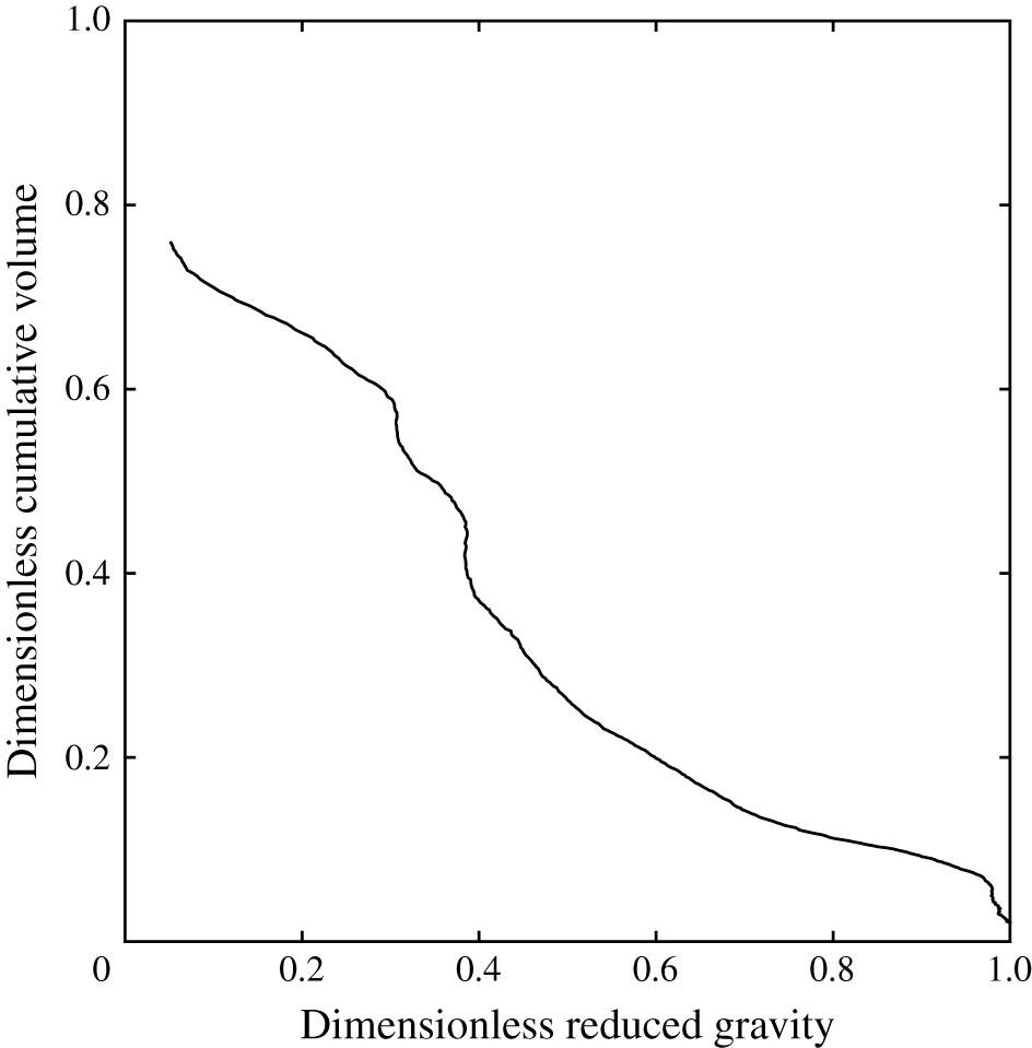
The traversing probe took measurements along a single line. To demonstrate that the profile taken along this line was representative of vertical profiles throughout the ponded region, a measurement of the density profile was made using a light attenuation technique. We added a constant concentration of methylene blue to the source fluid as a proxy for density. The technique measured the line-of-sight average dye concentration across the width of the tank (Cenedese & Dalziel Reference Cenedese, Dalziel, Carlomagno and Grant1998; Allgayer & Hunt Reference Allgayer and Hunt2012). The concentration field acquired by this method was then averaged over a 30 cm region along the tank adjacent to the profiler and filtered using a median filter with a 2 s time window to reduce the influence of random noise from the image sensor. The absolute density was not measured, meaning that this technique only showed the form of the density profile. The profile for the case with
 $Re_{s}=630$
at the time when the interface had reached the source is shown in figure 9. Despite the line-of-sight and along-tank averaging, the profile showed similar features to the density profile acquired by the traversing probe, as shown in figure 8(f). There was a homogeneous region at the bottom of the profile, and above this the ponded region was stratified. In the stratified part of the ponded region there were small regions of localised uniform density and weak static instability corresponding to those in the profile in figure 8(f). Averages over the large window width, shown in figure 9, showed less vertical structure than profiles taken over smaller window widths (not shown) or taken by the traversing probe. There was some horizontal variation in the small scale structure shown by averaging over narrow windows, but these variations were minimal and did not alter the large scale features discussed above. Note that a point-by-point comparison between the conductivity probe results and the ones obtained from light attenuation was not possible. Although the images were captured at eight-bit precision, the two or three least significant bits were affected by random noise and thus the light attenuation measurements required some degree of averaging to obtain the necessary precision.
Density profile measured using the light attenuation technique. The density is normalised against the peak value in the profile and the cumulative volume is normalised with the volume beneath the virtual origin.

5 Discussion
Modifying the persistently entraining model to allow fluid to peel away from the gravity current in stratified ambient fluid reduces the error and brings the functional form closer to the observed profiles. Segregation of fluid with different densities within the gravity current to different depths in the ambient fluid is supported by both the dye visualisations and the density profile measurements. Including an internal density structure within the gravity current is key to modelling the peeling detrainment behaviour, as also found by Cortés et al. (Reference Cortés, Rueda and Wells2014b ) for two-layer ambient stratifications. The excessive mixing of the persistently entraining model leads to ambient density profiles that are too homogeneous. Mixing is overestimated in the persistently entraining model because of two mechanisms. First, entrainment, as described by (4.1), continues as the gravity current moves through the stratified ponded region, mixing the current with the ambient more than in reality. Second, the model completely mixes the fluid within the gravity current by assuming a uniform, top-hat profile within the gravity current. The simplifying, end-member assumption made in the peeling detrainment model that no mixing occurs in the ponded region was a better approximation to mixing in the flow. Peeling detrainment also implies that, for gravity currents in stratified ambient fluid, substantially different flow pathways occur than suggested by persistently entraining models. Peeling detrainment, similar to that observed here in gravity currents, occurs in vertically falling plumes, but the peeling detrainment is less dominant (Wong et al. Reference Wong, Griffiths and Hughes2001). The stable stratification within the gravity current and the horizontal momentum of the mean flow in a gravity current, both absent in plumes, may increase the exchange by peeling detrainment in inclined gravity currents. The importance of these two effects requires further investigation.
The occurrence of detrainment for the regimes found in our experiments agrees with previous literature. The condition given by Baines (Reference Baines2005, Reference Baines2008) for the detraining gravity current behaviour to occur is that
 $$\begin{eqnarray}T\equiv C_{D}+1.2\times 10^{-4}Ri^{-1}-0.2(QN^{3}/g^{\prime })^{0.4}\sin \unicode[STIX]{x1D703}>0,\end{eqnarray}$$
where
 $C_{D}$
is the drag coefficient for the sloped surface and
 $N$
the local buoyancy frequency. In the present experiments, these parameter values were typically
 $C_{D}=0.006$
(as used by Baines (Reference Baines2005) for a smooth tank),
 $Ri=0.1$
,
 $Q=0.001~\text{m}^{2}~\text{s}^{-1}$
,
 $N=1~\text{s}^{-1}$
,
 $g^{\prime }=0.2~\text{m}~\text{s}^{-2}$
and
 $\unicode[STIX]{x1D703}=8.6^{\circ }$
, giving a value for
 $T$
of 0.0036. These values meet the criteria given by Baines (Reference Baines2005) for detraining gravity current behaviour.
The model and qualitative dye observations suggest the likely circulation and velocity field in the basin. This evidence is consistent with fluid from the internally stratified gravity current moving to different neutral buoyancy heights in the stratified region of the ambient fluid as the current descends the slope. This implies that the volume flux in the gravity current reduces as the current descends towards the bottom of the tank, as the outer layers of the gravity current leave the current to enter the stratified ambient fluid. This is in contrast to persistently entraining currents (Baines & Turner Reference Baines and Turner1969; Wells & Wettlaufer Reference Wells and Wettlaufer2005), where the gravity current volume flux increases towards the bottom of the basin as more fluid is entrained. The average volume flux in the ambient fluid is upwards and equal in magnitude to the downward flow in the gravity current, as required by volume conservation at any height in the basin. A similar trend of increasing and then decreasing volume flux in gravity currents on the Antarctic continental slope has been observed in field observations (Gordon et al. Reference Gordon, Orsi, Muench, Huber, Zambianchi and Visbeck2009).
Further work is needed to refine some of the assumptions made in the simple peeling model described here. In the ponded region, the gravity current fluid is assumed to move into the ambient fluid without any further mixing. In reality, some mixing continues to be driven by shear as the gravity current moves through the stratified ambient fluid. When the gravity current falls a large distance through a stratified ambient fluid, this neglected mixing will be a more significant source of error. A more sophisticated estimate of the continued mixing may potentially be made using the foundational work of Baines (Reference Baines2001), which gives methods to estimate the entrainment and detrainment coefficients. However, this extension is beyond the scope of the present work. The assumption of negligible drag in (4.2), whilst a good approximation to the laboratory experiments, may not be appropriate for many river inflows. River beds typically have shallower inclines and rougher surfaces than the case considered here in the laboratory. Including drag will change the fluxes along the gravity current and the density profile within the gravity current (Cortés et al. Reference Cortés, Rueda and Wells2014b ), but will not qualitatively change the peeling detrainment mechanism. Lakes are typically not uniform in temperature, even when they are at their most homogeneous before the summer stratification builds up. Initial stratification can prevent the gravity current from reaching the bottom of the lake. The expression in (4.27) could be extended, using a numerical implementation, to incorporate initial ambient stratification. Another important piece of future work is to incorporate peeling detrainment mechanisms into inflow parameterisations in operational field scale models and to validate the models. The most suitable sites for validation are lakes in which the evolution of the density profile from peeling detrainment is not influenced by other processes, such as strong wind driven internal seiches.
To show the potential influence of peeling detrainment in a geophysical example, we calculated the stratification that would be formed by a large, relatively cold river inflow of 100
 $\text{m}^{3}~\text{s}^{-1}$
at
 $4.5\,^{\circ }\text{C}$
into a well mixed lake with initial uniform temperature of
 $8.5\,^{\circ }\text{C}$
. The lake basin, of the same triangular geometry as our experiment, had depth 150 m, length 30 km, width 1 km and an incline of
 $0.3^{\circ }$
. A value of
 $E=3\times 10^{-3}$
was used, typical for a river inflow (Fernandez & Imberger Reference Fernandez and Imberger2006). These parameters give a virtual origin offset 13 m above the physical source. The basin would reach the
 $\unicode[STIX]{x1D70F}=1$
stratification, shown in figure 7(g), after 47 days. The persistently entraining gravity current model predicts a bottom water temperature of
 $7.8\,^{\circ }\text{C}$
whereas the peeling gravity current model predicts a bottom water temperature of
 $6.2\,^{\circ }\text{C}$
. In reality, river inflows are not constant in time. This variability, along with other influences present in the field such as solar heating and wind driven mixing, need also to be considered in field models of river inflows. The new predictions of the peeling detrainment model have wide ranging practical implications. In water resource management, dense inflows that fall to the bottom of stratified lakes can transport part of their dissolved constituents, such as pollutants or nutrients, into the surface and intermediate waters of lakes via detrainment mechanisms (Cortés et al.
Reference Cortés, Fleenor, Wells, de Vicente and Rueda2014a
). In building physics, peeling detrainment may explain why room stratifications are observed to have smoother density profiles than predicted by models that allow only entrainment and not detrainment. In oceanography, the peeling detrainment mechanism seen in these experiments supports observations of detrainment in the slope currents that form the downwelling limb of the meridional overturning circulation (Gordon et al.
Reference Gordon, Orsi, Muench, Huber, Zambianchi and Visbeck2009). Peeling detrainment is also likely to be found in smaller scale oceanic gravity currents, such as in the Southern Adriatic Pit (Bensi et al.
Reference Bensi, Cardin, Rubino, Notarstefano and Poulain2013), the Mediterranean outflow and effluent from desalination facilities (Fernández-Torquemada et al.
Reference Fernández-Torquemada, Gónzalez-Correa, Loya, Ferrero, Díaz-Valdés and Sánchez-Lizaso2009).
6 Conclusions
In this article, we investigated the evolution of the density profile in a basin fed with dense fluid by a gravity current. Dye visualisations of the filling flow show that fluid supplied by the source at the same instant went on to peel away from the gravity current and enter the stratified ponded region over a range of different depths and densities, in agreement with previous observations by Baines (Reference Baines2001). These visualisations are inconsistent with the prevailing model of a persistently entraining gravity current, which predicts that all the current fluid descends to the bottom of the basin and then upwells (Baines & Turner Reference Baines and Turner1969). We suggest that the observed peeling detrainment behaviour occurs because fluid within the gravity current, which itself is internally stratified, is neutrally buoyant across a range of depths within the stratified part of the ambient fluid. We proposed a model that incorporated the transport of fluid by peeling detrainment within the stratified portion of the basin. To incorporate peeling detrainment, the model includes information about the stratification within the gravity current. The peeling model gives good first-order descriptions of the shape and peak value of the observed ambient density profile. The model implies that the volume flux in the gravity current increases along the slope and then, once detrainment is active, the volume flux in the gravity current decreases. The proposed peeling detrainment model leads to a larger density gradient across the whole ambient fluid, also agreeing with observations. The model diverges from observations in low
 $Re_{s}$
runs, probably because the assumed linear density profile within the gravity current is a poor approximation to the true profile in these cases. The improved agreement in the new model is particularly good given the simple assumptions it uses. These laboratory results suggest that including a peeling detrainment model in field models would be valuable and could reduce the uncertainty in present predictions of downwelling currents in stratified basins in many important geophysical settings.
Acknowledgements
The authors are grateful to C. Caulfield, P. Linden, G. Lane-Serff, M. Hallworth and A. Wells for helpful discussions during the course of this research. The manufacturing skills of D. Page-Croft, C. Hitch and J. Milton were gratefully appreciated. C.A.R.H. gratefully acknowledges support by the Natural Environment Research Council (grant reference NE/H52449X/1) and Arup. H.E.H. is grateful for support from a Royal Society Wolfson Research Merit Award and a Leverhulme Emeritus Research Fellowship. The density profile measurements that formed the basis of this analysis are openly available at the website http://www.repository.cam.ac.uk/handle/1810/249124.
Supplementary movie
A supplementary movie is available at https://doi.org/10.1017/jfm.2017.196.