INTRODUCTION
Since the adoption of genetically modified (GM) crops started in 1996, both the global area and the number of countries adopting GM have increased continuously. The worldwide area covered by GM crops is 148 million ha (James Reference James2011); the USA is the main GM producer with 66·8 million ha allocated to GM crop production, followed by Brazil (25·4 million ha), Argentina (22·9 million ha), India (9·4 million ha) and Canada (8·8 million ha).
The two main agronomic traits introduced by genetic engineering that are being commercialized are herbicide-tolerant (HT) and insect-resistant (Bt) crops. The dominant trait is HT crops (89·3 million ha), which refers to crops that have been made resistant to a particular herbicide either by incorporating a new gene into a crop or switching off an existing gene, followed by Bt crops (26·3 million ha). Genes transferred from the soil bacterium Bacillus thuringiensis are responsible for insect resistance among transgenic plants. The combination or ‘stacking’ of both traits is growing rapidly, and covered over 0·22 (32·3 million ha) of the global biotech crop area in 2009 (James Reference James2011).
The main GM crops that are being cultivated are HT soybeans, occupying 73·3 million ha (0·50 of the global area), followed by GM (i.e. HT and Bt) maize with 46·8 million ha (0·31), GM cotton with 21 million ha (0·14) and HT oilseed rape with 7 million ha (0·05).
The rapid adoption of HT and Bt technologies by farmers is a result of the many benefits associated with GM crops. GM profits are usually higher than those achieved by conventional varieties due to the combination of yield protection and lower production costs. HT technologies do not increase yields significantly but their use facilitates more cost-effective weed control. Bt crops increase farmers’ profits as a result of higher yields and lower expenditure on insecticides (Qaim Reference Qaim2009; Ervin et al. Reference Ervin, Carrière, Cox, Fernández-Cornejo, Jussaume, Marra, Owen, Raven, Wolfenbarger and Zilberman2010). More effective management of weeds and insects means that farmers may promote the adoption of conservation tillage (i.e. minimum tillage or direct sowing) and/or reduce the number of insecticide sprays used. This translates into cost savings, i.e. lower pesticide costs and lower labour, machinery and fuel requirements (Ervin et al. Reference Ervin, Carrière, Cox, Fernández-Cornejo, Jussaume, Marra, Owen, Raven, Wolfenbarger and Zilberman2010). However, expected benefits of GM crops vary greatly by region, depending on pest infestation levels and seed and technology costs. In most cases, GM seed costs are greater than conventional seed costs, so a certain pest infestation level is required for farmers to obtain economic benefits from GM adoption. The higher the infestation level is the greater the reduction in crop losses and pesticide costs (Klotz-Ingram et al. Reference Klotz-Ingram, Jans, Fernandez-Cornejo and McBride1999).
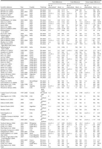
Several studies on economic impacts of GM crops have been conducted in specific countries at the farm level (see Table 1 below for a selection of studies). However, very few studies have focused on analysing the economic performance of GM crops worldwide (Brookes & Barfoot Reference Brookes and Barfoot2005; Qaim Reference Qaim2009; Carpenter Reference Carpenter2010). While Brookes & Barfoot (Reference Brookes and Barfoot2005) and Qaim (Reference Qaim2009) compiled data from a number of studies on the economic impact of commercialized GM crops, Carpenter (Reference Carpenter2010) extended the analysis to include a greater number of observations and carried out statistical analyses of yields and gross margins. Carpenter's analysis suggested that the benefits of growing GM crops compared with the benefits of growing conventional crops are positive for most countries, with few exceptions.
Number of observations of economic and agronomic performance per scientific reference

* Positive or negative variation GM v. non-GM.
† NA, not available.
Carpenter (Reference Carpenter2010) examined the impact of commercialized GM crops in yields and gross margins for developing and developed countries, but failed to provide any insight on production costs nor distinguished between the two traits (Bt and HT crops). For instance, Carpenter (Reference Carpenter2010) concluded that GM crops have, on average, greater yields than conventional crops, but it cannot be inferred from the results whether this occurs for both traits commercialized in GM crops, or whether these yield differences are statistically significant. Some other studies concluded that yield differences between GM and conventional crops do not occur for HT but do for Bt crops (Qaim Reference Qaim2009; Ervin et al. Reference Ervin, Carrière, Cox, Fernández-Cornejo, Jussaume, Marra, Owen, Raven, Wolfenbarger and Zilberman2010). In order to tackle this issue and overcome the limitations of Carpenter's analysis (Carpenter Reference Carpenter2010) of the economic and agronomic performance of GM crops, the present analysis was extended by splitting each variable up (yields, production costs and gross margins) into GM traits. The analysis was applied at developing/developed country level as well as at world region level, thus creating a new array of variables to be analysed.
As pointed out above, the reasons behind the rapid expansion of GM crops worldwide are partially explained by the greater advantages and economic benefits associated with them. However, the debate on whether adopting GM crops leads to a relatively higher agronomic and economic performance is still ongoing and there is no agreement within the scientific community. By conducting a meta-analysis, which reviews and combines the results of 56 scientific studies (i.e. scientific publications and governmental reports), the present paper informs this debate. In particular, the following issues regarding the impact of commercialized GM crops are examined. Firstly, the question of whether GM crops perform better than non-GM crops is examined. If GM crops perform better than non-GM crops, this would partially explain the current level of adoption of GM crops worldwide and prospective adoption levels can be expected to be high. Secondly, the relative performance of Bt and HT crops compared with conventional crops is examined. Conducting the analysis at trait level allows discernment of cases where any advantage associated with GM crops is mainly due to only one trait. In such cases, it is interesting and appropriate to provide precise information on the performance of each trait, since aggregating them into GM crops would misrepresent GM crop performance. Thirdly, the performance of GM crops in developing countries compared with in developed countries is examined and, finally, whether some world regions achieve better results than others in terms of yields, production costs and gross margins. The same reasoning used in the second point above applies to the analysis at country's development and regional levels.
MATERIALS AND METHODS
Dataset
Several studies based on sample surveys compared the economic and agronomic performance of GM crops (HT, Bt and stacked (the stacked-gene trait is a combination of two transgenic traits, Bt and HT)) and non-GM crops at farm level in different countries (see Table 1). Data on yield, production cost and gross margin of GM and conventional crops were collated from these studies to carry out the analysis (data published more than once were only included once in the dataset for the statistical analysis). These data allowed calculation of the absolute difference in yields, production costs and gross margins, between GM crops and conventional crops as shown in Eqn (1) below.
 $$\Delta Y_i = x_{{\rm GM} _i} - x_{{\rm non - GM} _i} $$
where ΔY i is the unweighted difference of the variable of interest between GM and non-GM crops in study I; x GM represents the yield, production cost or gross margin of a certain GM crop and x non-GM represents the yield, production cost or gross margin of the conventional counterpart. Using absolute differences required unit harmonization (i.e. same monetary and weight units). Data collated included different measurement units for yield, production costs and gross margin. Currency units were normalized to €/ha and deflated using year 2000 as the base year, while yield units were normalized to tonnes/ha. The absolute difference of these agronomic and economic measures obtained from Eqn (1) can be used for further analysis.
Table 1 gives information on the literature consulted in order to compile a total of 97 observations on gross margin absolute differences between GM and conventional crops, 133 observations on yield absolute differences and 104 observations on cost absolute differences. These observations covered different GM traits and crops (Bt cotton, stacked-gene cotton, HT oilseed rape, HT soybeans, Bt maize, HT maize) during several seasons (1996–2007) and in 16 countries.
To carry out the analysis, countries were grouped into developing or developed countries following the International Monetary Fund's (2009) classification. According to this, Argentina, Chile, China, India, Mexico, Mozambique, the Philippines, Romania and South Africa were considered as developing countries, whereas Australia, Canada, the Czech Republic, France, Portugal, Spain and the United States were treated as developed countries. In addition to this, spatial classification of data another categorization was carried out considering world regions (Africa, Asia, Australia, Europe, North America and South America).
Methodology
Two approaches, weighted and unweighted, can be used when conducting a meta-analysis. The weighted approach is used to give more weight to the information provided by studies with large samples, so in the present study a weighted approach was used to minimize the impact of a small number of studies with small sample sizes. Weights were based on the assumption that:
 $$\Delta Y_i \sim N\left( {\mu, \displaystyle{{\sigma ^2} \over {n_i}}} \right){\rm,} \quad i = 1, \ldots ,I;\quad \sum {n_i = N} $$
where the absolute difference of the variable of interest follows a normal distribution with mean μ and variance σ 2/n i, where n i is the number of observations for study i. While standard errors of means (s.e.m.) are commonly used when combining estimates across studies, this was impracticable in the present study due to the lack of information on standard deviations and standard errors in a relatively large number of studies. Other alternative approaches, such as making variance country specific, are valid for tackling heterogeneity. Heterogeneity problems are common in cDNA and animal breeding literature where individual variance estimators (Cui et al. Reference Cui, Hwang, Qiu, Blades and Churchill2005) and ways to identify sources of variation of heterogeneity (Foulley & Quaas Reference Foulley and Quaas1995) have been developed.
Bayesian methods were used for making inferences about both the economic (i.e. gross margin and production cost) and agronomic performance (i.e. yield) of GM crops in comparison with non-GM crops across different geographical levels and commercialized crops. The Bayesian approach differs from the classical approach in that it treats parameters as random variables and yields distributional information. The technical core of Bayesian inference is summarized in the following expression, which represents Bayes theorem:
 $$p(\theta |y) \propto p(\theta )p(y|\theta )$$
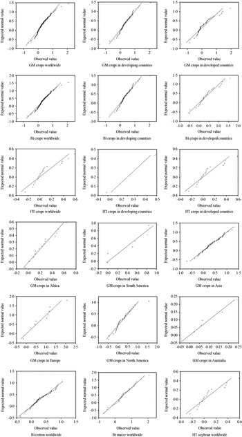
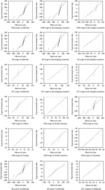
where p(θ|y) is the posterior probability density function (pdf) for the parameter vector θ, given the sample information y, p(θ) is the prior information for the parameter vector θ and p(y|θ) is the likelihood function, which is a pdf for the observations given the parameters. The posterior pdf is used in the Bayesian approach to make inferences about the parameters of interest, which in the present analyses were the means of a set of variables (i.e. absolute difference in gross margin, yield and production cost between GM and non-GM crops). Therefore, a number of analyses were conducted using Bayesian methods to evaluate the relative performance of GM crops at different levels (see Table 2). The analyses of the variables of interest were carried out in three different ways, depending on the assumption regarding the errors, viz. normally distributed errors, Student's t distributed errors or no distribution assumed. The choice of which method to use was based on whether errors were normally distributed using test for normality. In addition to the Bayesian analysis, classical parametric t tests and non-parametric Wilcoxon signed-rank tests were carried out for comparison. The non-parametric Bootstrapping residuals method (Efron & Tibshirani Reference Efron and Tibshirani1993), a resampling method for statistical inference where no distributional parameters are assigned, was used to estimate μ and the probability of the variables of interest being greater than zero for cases where the distribution of ΔY was skewed. Skewness was tested by examining normal quartile–quartile (QQ) plots (see Figs 1–3), which compared the distribution of a variable to the normal distribution, and by calculating the sample skewness statistic  ${\rm ss} = m_3 /m_2^{3/2} $ where m 3 is the sample third central moment and m 2 is the sample variance. If the value of the estimate of skewness exceeds 2 × the standard error of skewness (calculated as
 ${\rm SES} = \sqrt {6/N} $) then the sample distribution is regarded as skewed (Tabachnik & Fidell Reference Tabachnik and Fidell1996) and non-parametric Bootstrap is carried out. The QQ-plots in Figs 1–3 show that while differences in gross margin and yields are close to normality, absolute differences in costs (Fig. 2) are heavily skewed to the left in cases such as GM crops worldwide, GM crops in developing countries, Bt crops worldwide and Bt crops in developing countries. This skewness is due to a number of observations taken from studies in China (Pray et al. Reference Pray, Ma, Huang and Qiao2001; Huang et al. Reference Huang, Hu, Fan, Pray and Rozelle2002a), where the purchase of pesticides for conventional cotton were reported to incur relatively high costs; more specifically, these authors report up to ten times higher pesticide costs for conventional than for Bt cotton (Pray et al. Reference Pray, Ma, Huang and Qiao2001; Huang et al. Reference Huang, Hu, Fan, Pray and Rozelle2002a).
QQ-plots for absolute differences in yields.

QQ-plots for absolute differences in costs.

QQ-plots for absolute differences in gross margin.

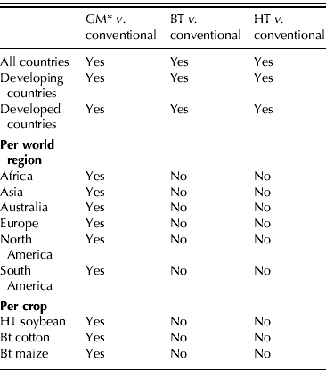
Analysis conducted for gross margin, yield and production cost differences
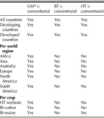
* GM crops include Bt and HT traits.
In order to check the consistency of the model to the data, graphical posterior predictive checks and a sensitivity analysis were conducted to assess the effect of alternative analyses on the posterior inferences (i.e. how much posterior inferences change when other probability models are used).
Normally distributed errors
For each variable (e.g. yield absolute difference between GM and conventional crops) there are N independent observations y′ = (y 1,y 2,…,y N), which are assumed to be drawn from a Normal population with unknown mean μ and variance σ 2/n i where n i is the number of observations for study i. Therefore, each variable equals its mean (e.g. the mean of absolute difference yield between GM v. conventional crops) plus some zero-centred normally distributed error term  $\varepsilon _i \sim N(0_N, h^{ - 1} I_N /n_i )$ where h = 1/σ 2 is the error precision and I N is the N×N identity matrix. This assumption on the error term is analogous to approaches such as the method of weighted least squares (Whitehead Reference Whitehead2002). Thus, y i=μ+ε i where y is a vector of data of the absolute difference of agronomic and economic measures between GM and conventional crops. Under the assumption of constant σ 2,
 ${\rm Var(}\varepsilon _i {\rm )} = \sigma ^2 /n_i = h^{ - 1} I_N /n_i $; therefore the homoskedastic version of the model should be
 $\sqrt {n_i} y_i = \mu \sqrt {n_i} + v_i $ with Var(v i)=σ 2 and
 $v_i = \varepsilon _i \sqrt {n_i} $. The transformed model can be written as
 $y_i^* = \sqrt {n_i} \mu + v_i $. The aim is to estimate the posterior distribution of the unknown mean μ of the absolute difference of agronomic and economic measures (yield, production costs and gross margin) between GM and conventional crops. The assumption about the errors (i.e. normally distributed) defines the likelihood function. Thus, assuming
 $v\sim N(0_N, h^{ - 1} I_N )$ means that the likelihood function can be written as
 $$p\left( {y^* |\mu, h} \right)\! =\! \displaystyle{{h^{N/2}} \over {\left( {2\pi} \right)^{^{N/2}}}} \exp \left(\! { - \displaystyle{h \over 2}\left( {\sum\limits_{i = 1}^N {y_i^*} - \sqrt {n_i} \mu} \right)^2} \right)$$
As shown in Eqn (3), in order to conduct Bayesian inference the likelihood function must be complemented with a prior distribution on the parameters μ and h. Usually, particular classes of prior distributions are chosen with the aim of facilitating interpretation and/or making computation easier. An independent Normal-Gamma prior was used for the mean μ and error precision h for the same reasons of simplicity. These are natural conjugate prior distributions, which, when combined with the likelihood, yields a posterior distribution that falls in the same class of distributions:
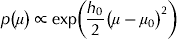 $$p\left( \mu \right) \propto \exp \left( {\displaystyle{{h_0} \over 2}\left( {\mu - \mu _0} \right)^2} \right)$$
where μ 0 and h 0 are the mean prior and inverse variance prior distributions, with values of 0 and 0·0001, respectively, making the prior non-informative (i.e. the mean prior of the absolute difference was given a variance of 10 000 units (t/ha or €/ha depending on the variable studied), which effectively means that no prior information about this parameter was used).
 $$p\left( h \right) \propto h^{a - 1} \exp \left( { - \displaystyle{a \over c}} \right){\rm,} \; h \gt 0$$
where a and c are hyperparameters with values of 0·05 and 5 for yield absolute difference, respectively, which made the prior non-informative. The parameterization of the gamma distribution is  $G(\theta |a,c) = {\textstyle{1 \over {\Gamma \left( a \right)c^a}}} \theta ^{a - 1} {\rm e}^{ - \theta /c} $. Errors in absolute yield difference were expected to be of the order of magnitude of 1–2 t/ha and maybe five at most. This suggested that the standard deviation might be c. 2 and error precision h = 1/22 = 0·25, if errors were normally distributed with mean zero. Hence, it was assumed that the error precision h∼G(a,c) with mean ac = 0·25 and variance ac 2 = 1·25 (i.e. hyperparameters are a = 0·05 and c = 5). The hyperparameters a and c took values of 0·05 and 1000, respectively, for the absolute difference of economic measures (production cost and gross margin) h∼G(0·05, 1000). These values were based on the ‘crude’ assumption that errors in production cost and gross margin differences were of the order of magnitude of tenths of euros per hectare, being the mean and the standard deviation 50 €/ha (i.e. error precision h = 0·0004). More importantly, little weight was attached to the prior information, since values assigned to the hyperparameters of the error precision made the prior relatively non-informative.
As in Eqn (2), the joint posterior distribution was defined by the product of the likelihood times the priors.
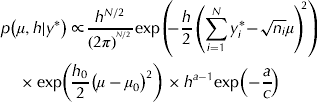 $$\eqalign{ & p\left( {\mu, h|y^*} \right) \propto \displaystyle{{h^{N/2}} \over {\left( {2\pi} \right)^{^{N/2}}}} {\rm exp}\left(\!\! { - \displaystyle{h \over 2}\left( {\sum\limits_{i = 1}^N {y_i^*\! -\! \sqrt {n_i} \mu}} \right)^{\!\!2}} \right) \cr & \quad \times {\rm exp}\left( {\displaystyle{{h_0} \over 2}\left( {\mu - \mu _0} \right)^2} \right) \times h^{a - 1} {\rm exp}\left( { - \displaystyle{a \over c}} \right)} $$
Under the Bayesian approach, the posterior inference was based on the conditional distributions of the parameters given the observables. The aim was to obtain the conditional posterior distribution of the mean of the absolute difference, enabling inferences to be made about the means of the variables of interest. For instance, the means of the absolute difference in gross margin between GM and conventional crops between geographical regions in the world could be compared. The Bayesian computation of the conditional posteriors was done using a Gibbs sampler (Geman & Geman Reference Geman and Geman1984). A total number of 5100 random draws were generated from the conditional distributions with 100 draws discarded and 5000 retained. These 5000 draws could be considered a sample from the joint posterior density function of the parameters.
The conditional posterior distributions for μ and h followed normal and gamma distributions, respectively, since independent Normal-Gamma natural conjugate priors for the mean μ and error precision h were selected.
Student's t-distributed errors
So far it has been assumed that the errors followed a Normal distribution. However, this may not be realistic when analysing data from different geographical regions of the world, because different conditions existing in those regions (e.g. different crop prices, different conventional pest treatments, etc.) may produce heteroskedasticity, i.e. different error variances across observations (e.g. across geographic regions). Therefore, the normality assumption in the errors were relaxed in those cases where normality tests rejected normality, by assuming the less restrictive Student's t distribution, which is effectively the same as considering that variances differ across observations. Effectively, the Student's t distribution is a weighted average of different Normal distributions which have different variances but the same means.
The problem with accounting for heteroskedasticity is the same as for the normally distributed errors, except that now  $v_i \sim N(0_N, h^{ - 1} \lambda _i^{ - 1} )$ is assumed instead of
 $v_i \sim N(0_N, h^{ - 1} I_N )$ for i = 1, …, N, where
 $\lambda = (\lambda _1, \lambda _2,\ldots, \lambda _N )'$ is a vector of error precisions. Following Koop (Reference Koop2003), when the form of the heteroskedasticity was unknown a new parameter λ was incorporated into the Bayesian analysis to introduce heteroskedasticity, of which the prior was Gamma distributed,
 $p(\lambda ) = \prod _{i = 1}^N f_G (\lambda _i |1,\upsilon _\lambda )$, and depended on the hyperparameter υ λ. As in Koop (Reference Koop2003), an exponential distribution was used for the prior of υ λ, which depended on the hyperparameter υ λ. We set υ λ = 25 which allocated substantial prior weight to both fat-tailed error distributions as well as error distributions which were roughly Normal (Koop Reference Koop2003).
The conditional posterior distribution of the new parameters λ i had the form of a Gamma density, whereas the conditional posterior distribution for υ λ was not a standard one and a Random Walk Chain Metropolis–Hastings algorithm (Hastings Reference Hastings1970; Chib & Greenberg Reference Chib and Greenberg1995) was used to obtain the distribution:
 $$p\left( {\lambda _i |y^*, \mu, h,\upsilon _\lambda} \right) = f_G \left( {\lambda _i |\displaystyle{{\upsilon _\lambda + 1} \over {hv_i^2 + \upsilon _\lambda}}, \upsilon _\lambda} \right)$$
 $$p\left( {\upsilon _\lambda |y^*, \mu, h,\lambda} \right) \propto \left( {\displaystyle{{\upsilon _\lambda} \over 2}} \right)^{N\upsilon _\lambda /2} \Gamma \left( {\displaystyle{{\upsilon _\lambda} \over 2}} \right)^{ - N} \exp \left( { - \eta \upsilon _\lambda} \right)$$
where
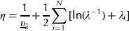 $$\eta = \displaystyle{1 \over {\underline \upsilon _\lambda}} + \displaystyle{1 \over 2}\sum\limits_{i = 1}^N {[{\rm ln}(\lambda ^{ - 1} ) + \lambda _i ]} $$
The conditional posterior distributions for the mean μ, error precision h and λ of each variable (i.e. yield, production costs and gross margin) for each case study (traits, country-development level, geographical region and crop) were obtained using a Gibbs sampler in the same way as in the previous section. The conditional posterior distributions provided information on the absolute difference of economic and agronomic performance measures of GM crops at different geographical levels. In addition, obtaining the conditional posterior distributions allows comparisons to be made between Bt and HT traits, between developing and developed countries, and between geographical regions and between crops. The results from such comparisons were examined and are presented in the next section.
Bootstrapping residuals
The Bootstrap sampling consisted of (i) calculating approximate errors using the least square estimate of μ  $(\hat \mu )$; (ii) drawing the approximate errors 5000 times with replacement to obtain
 $v_i^{**} $ and (iii) using these to generate
 $y_i^{**} = \hat \mu + v_i^{**} $.
Other statistical tests
The data were also compared using classical t tests and non-parametric Wilcoxon signed-ranked tests in comparison to the Bayesian results. The linear regression model  $y_i^* = \sqrt {n_i} \mu + v_i $ was also fitted using the least squares approach from which the mean μ of the absolute difference of agronomic and economic measures (yield, production costs and gross margin) between GM and conventional crops was estimated. This was done for those cases where the distribution of errors was Normal. Student's t tests were used to test the null hypothesis H 0:μ = 0 againstH 0:μ≠0. When normality of errors was not assumed Wilcoxon signed ranked tests were conducted. Unweighted absolute differences were used here since this is a non-parametric test and weighted differences were obtained through the variance.
RESULTS
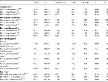
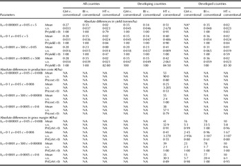
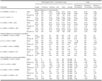
This section reports the results of Bayesian and bootstrapping analyses for the difference of gross margin, yield and production costs between GM and conventional crops. Tables 3–5 show the estimated means of the conditional posterior distribution, as well as the probability of the posterior distribution of the mean of the absolute difference of yield, production cost and gross margin between GM and non-GM crops at worldwide level being above 0 (i.e. the probability of GM crops performing better than conventional ones). The tables also show results (i.e. mean, standard deviation and probability of μ being greater than zero) obtained by conducting bootstrap sampling of the residuals with replacement 5000 times for cases where distributions were skewed. These results are illustrated per country-development level, per geographical region and for specific commercialized GM crops (HT soybeans, Bt cotton and Bt maize). The results from t tests and Wilcoxon signed ranked tests agree with the results obtained from the Bayesian approach.
Mean and standard deviation of conditional posterior distributions of absolute difference of the yield between GM and conventional for countries and crops

* For n > 20, the Wilcoxon test statistic is normally distributed with mean n(n + 1)(2n + 1)/24, hence the P-value can be determined by comparing  $Z = [W - n(n + 1)/4]/\sqrt {n(n + 1)(2n + 1)/24} $ where, W is the Wilcoxon test statistic.
† N Normal distribution, NN Non-Normal distribution, * Bootstrapping.
‡ GM crops include Bt and HT traits.
§ NA, not applicable.
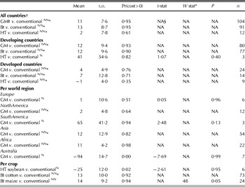
Mean and standard deviation of conditional posterior distributions of absolute difference of production costs between GM and conventional for countries and crops

* For n > 20, the Wilcoxon test statistic is normally distributed with mean n(n + 1)(2n + 1)/24, hence the P-value can be determined by comparing  $Z = [W - n(n + 1)/4]/\sqrt {n(n + 1)(2n + 1)/24} $, where W is the Wilcoxon test statistic.
† N Normal distribution, NN Non-Normal distribution, * Bootstrapping.
‡ GM crops include Bt and HT traits.
§ NA, not applicable.
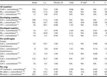
Mean and standard deviation of conditional posterior distributions of absolute difference of the gross margin between GM and conventional for countries and crops

* For n > 20, the Wilcoxon test statistic is normally distributed with mean n(n + 1)(2n + 1)/24, hence the P-value can be determined by comparing  $Z = [W - n(n + 1)/4]/\sqrt {n(n + 1)(2n + 1)/24} $, where W is the Wilcoxon test statistic.
† N Normal distribution, NN non-normal distribution, *bootstrapping.
‡ GM crops include Bt and HT traits.
§ NA, not applicable.
Yield
Table 3 shows the mean and standard deviation of the conditional posterior distributions obtained for the weighted mean of the absolute difference in yield between GM and conventional crops. The probability of GM crops performing better agronomically than conventional crops was calculated: by examining the output of the conditional posterior distribution the posterior mass above zero can be calculated to examine whether the posterior distributions of the absolute difference in yield between GM and conventional crops were above zero. The mean, standard deviation and probability of μ being greater than zero of the absolute difference in yield between GM and conventional crops for cases where the distribution of ΔY was skewed is also reported. Table 3 also shows results of t tests and Wilcoxon tests for comparison with the Bayesian results. Overall, GM crops as a whole gave higher yields than non-GM crops regardless of the country-development level (>0·95 of the conditional posterior distribution was above zero). Regarding the traits, while the agronomic performance of Bt crops was undoubtedly better than their conventional counterparts, there are some doubts about the performance of HT crops over conventional crops. The results show that there was no difference between Bt and HT traits relative to non-GM crops in terms of agronomic performance when analysis was conducted for developing countries (<0·95 conditional posterior distribution above zero). The conditional posterior distributions of yield differences for HT and Bt traits in developing countries were compared, with no differences found. However, Bt crops were found to perform better than HT crops in developed countries (>0·95 conditional posterior distribution above zero). On average, GM crops yielded 0·35 and 0·25 t/ha more than conventional crops in developing and developed countries, respectively. Less developed regions such as South America, Asia and Africa achieved, on average, similar absolute differences in yield between GM and conventional crops than ‘developed regions’ such as Australia, North America and Europe (see Table 3 and Fig. 4).
Density plots and raw data histograms for absolute differences in yields.

Regarding the commercialized crops studied (HT soybeans, Bt cotton and Bt maize), Bt cotton and Bt maize reached higher yields on average than their conventional counterparts (0·30 and 0·55 t/ha, respectively). Differences in yield performance relative to non-GM crops were found between these three crops, with Bt maize performing best, followed by Bt cotton.
Production cost
The absolute differences in costs of production between GM and non-GM crops were examined (Table 4). The effect on production costs of adopting GM crops had two aspects: a reduction in costs due to savings in pesticides and an increase in costs due to higher GM seed prices. It was found that the cost associated with adopting GM technologies was higher than for the conventional varieties when all countries were considered, ranging from 2 to 12 €/ha. This means that the potential savings in pesticide use offered by the new technology were more than offset by the higher price associated with the GM seeds. However, no cost differences were found between HT traits and their conventional counterparts in either developing or developed countries. However, because of the low number of observations available, this result needs to be treated with caution. When comparing Bt and HT crops, no significant (i.e. <0·90 of the conditional posterior distribution was above zero) differences relative to non-GM crops were found in the production costs associated with these traits in developing or developed countries (comparisons between conditional posterior distributions of production costs differences for HT and Bt traits in both developing and developed countries were conducted).
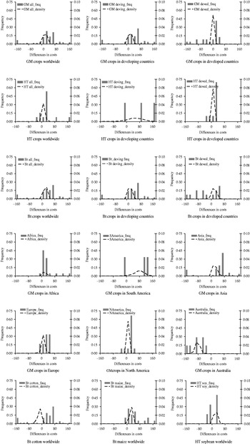
Absolute differences in production costs between GM and conventional crops were found to be higher in developing countries than in developed countries, because the production costs associated with growing HT crops are even lower than growing conventional crops (Fig. 5). This may be because (i) chemical pesticides used in developing countries are possibly inexpensive and outdated (Ecobichon Reference Ecobichon2001) and (ii) possible differences in seed prices charged in developing and developed regions. Pretty et al. (Reference Pretty, Morison and Hine2003) showed that farmers in the poorest countries tended to buy inexpensive and old chemical pesticides because they lacked the money to invest in costly inputs and technologies. The regions where this difference in production costs was highest were South America (65 €/ha) and Asia (12 €/ha), with differences in the production costs of GM crops in Australia being significantly lower (P < 0·10) than the production costs of conventional crops (−94 €/ha; Fig. 5). Farmers in developing countries may encounter economic difficulties when adopting GM technology due to the higher costs associated with adopting the new technology. Despite the fact that adoption of GM crops may reduce the number of pesticide applications (Falck-Zepeda et al. Reference Falck-Zepeda, Traxler and Nelson2000a), seed prices more than offset such benefits. Thus, seed prices may act as a barrier to adopting the new technology for many farmers in developing countries.
Density plots and raw data histograms for absolute differences in costs.

Focusing on the main GM crops (HT soybeans, Bt cotton and Bt maize), the production costs of Bt cotton and Bt maize were, on average, 13 and 14 €/ha higher, respectively, than for their conventional counterparts whereas absolute differences in the production costs for HT soybeans were 25 €/ha lower than for conventional soybean on average. The absolute difference in production costs between HT and conventional soybeans was significantly lower (P < 0·10) than the absolute difference in production costs between Bt cotton and Bt maize and their conventional counterparts.
Gross margin
Table 5 shows the mean and standard deviation of the conditional posterior distributions obtained for the mean of the absolute difference of the gross margin between GM and conventional crops. The probability of GM crops performing better than conventional ones was calculated to examine whether the posterior distributions of the absolute difference of gross margin between GM and conventional crops were above zero (i.e. GM crops performed better economically than conventional crops). The results show that, on average, GM crops outperformed non-GM crops in terms of gross margin regardless of trait when all countries are included in the analysis. Carpenter (Reference Carpenter2010), by counting the positive, neutral and negative results regarding gross margins (economic performance), also concluded that GM growers performed better economically (larger differences in gross margins) than conventional growers. However, Carpenter's approach did not allow any possibility of investigating whether differences in economic performance exist between GM traits and their conventional counterparts.
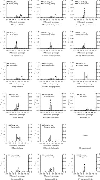
Table 5 and Fig. 6 show that GM crops economically outperformed non-GM crops in both developing and developed countries, this difference being more pronounced for farmers in developing countries. In this regard, it was found that while Bt traits performed economically better than conventional crops in both developing and developed countries, HT crops achieved on average greater gross margins than conventional crops. However, uncertainty over HT incomes in developed countries was too large for any difference between HT and conventional income to be statistically significant. Although this seems to contradict Carpenter's (Reference Carpenter2010) suggestion that more positive impacts of HT crops are expected with respect to conventional crops, the present results need to be treated with caution because the number of observations is low. When comparing Bt and HT crops, significant differences (P < 0·10) relative to non-GM crops were found in gross margins associated with these traits in developing and developed countries.
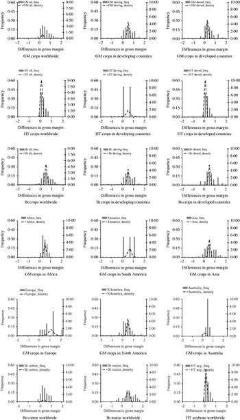
Density plots and raw data histograms for absolute differences in gross margins.

In addition to obtaining the conditional posterior distribution for the mean absolute difference of gross margin between GM and conventional crops for all countries and country-development levels, the analysis was also conducted on five geographical regions. All showed significantly higher gross margins for GM crops than for conventional varieties (>0·90 of the conditional posterior distribution was above zero). Geographical regions where absolute differences in gross margin between GM and conventional crops were greater were Asia (135 €/ha), Africa (76 €/ha) and Europe (65 €/ha), Asia being significantly different from Europe (>0·90 of the conditional posterior distribution was above zero; Fig. 6).
An analysis of the gross margin per crop, focusing on the main GM crops in terms of cultivated area, was also conducted to investigate whether these commercialized GM crops had any advantage over their conventional counterparts and whether there was any difference between them. The results showed that all crops performed better economically than their conventional counterparts, with both Bt cotton and Bt maize performed better than HT soybeans (>0·99 of the conditional posterior distribution was above zero; Table 5 and Fig. 6).
Which trait (Bt or HT) performed better in terms of gross margins was also investigated. In this regard, it can be concluded that Bt crops perform better than the other (>0·90 of the conditional posterior distribution was above zero), and adopting Bt or HT crops had a positive impact on farmers’ gross margins.
Sensitivity analysis
In order to check the consistency of the model to the data, graphical posterior predictive checks were conducted. Figures 4–6 display 18 densities, each of which represents conditional posteriors of the mean of the absolute difference of the measures studied superimposed on histograms of actual data. All densities are located within reasonable bounds (i.e. the model fits to the data).
A sensitivity analysis was conducted to examine the impact of alternative prior specifications on the posterior inferences (Tables 6 and 7). The priors reflected the subjective distributions prior to empirical evidence. Therefore, it was not the aim to start with an informative prior that reflected empirical evidence but rather a relatively diffuse prior that would be dominated by the data. Therefore, the point of the sensitivity analysis was to show that the priors have a relatively minor role. Alternative values were assigned to the hyperparameters h 0, a and c associated with the error precision of the normal and the mean and variance of the gamma distribution of the differences in yield, production costs and gross margin. In particular, the prior assumptions were changed by (i) setting the error precision of the mean μ to h 0 = 0·000001 to check that using a less informative prior for the mean did not change the results; (ii) setting the error precision of the h 0 = 0·1 which means a relatively low standard deviation (i.e. it was assumed that the variance of the mean is 10 units (t/ha or €/ha depending on the variable studied), which effectively meant giving strong prior information about this parameter), keeping the mean and variance of the gamma distributions for absolute differences between yields, production costs and gross margins the same; (iii) keeping the error precision at h 0 = 0·0001 and varying the mean of the gamma distribution for absolute yield differences from 0·25 to 25 and varying the mean of the gamma distribution for absolute production costs and gross margin differences from 0·0004 to 0·04 in both cases; (iv) keeping the error precision at h 0 = 0·0001 and varying the variance of the gamma distribution to from 1·25 to 125 for absolute yield differences and from 50 000 to 5 000 000 for absolute production costs and gross margin differences. Tables 6 and 7 show model results for all cases studied. The results from the sensitivity analysis were consistent with the analysis carried out. A notable result is that when the error precision of the mean μ was set to h 0 = 0·1 the mean tended to be closer to zero. This result was expected for cases where the results obtained in the analysis showed that the absolute difference in yield, production costs and gross margin is over 5–10 absolute units. This occurred because of the strong assumption that the absolute difference is zero (i.e. a small variance of 10 was set).
Sensitivity analysis I

* NA, not applicable.
Sensitivity analysis II

* NA, not applicable.
Therefore, based on the results obtained from the graphical check and sensitivity analysis the data do not appear to contradict the model and the inferences from the model make sense.
DISCUSSION
The agronomic and economic performance of GM crops worldwide was analysed using Bayesian, classical and Bootstrap sampling statistics. The statistical treatment of the collated information allowed comparisons to be made between GM and conventional crops in probabilistic terms on a number of economic and agronomic performance measures. The approach used to analyse GM crops expanded on and complemented previous analyses by using robust statistical techniques that allowed comparisons between the main GM commercialized crops, country-development levels and geographical regions.
It is concluded that in general GM crops performed better economically than non-GM crops, mainly due to the greater yields obtained by GM crops, despite production costs usually being higher for the GM variety. Although this statement can be generalized for the Bt trait, some exceptions were found when comparing HT v. conventional crops. It is worth noting that although it cannot be discerned whether the advantages of cultivating GM crops were due to the technology itself or to farmers’ managerial skills (GM adopter effect), the GM adopter effect is expected to diminish as the technology advances.
A clear outcome of the meta-analysis conducted is that developing countries outpace developed countries when comparing GM (Bt or HT) crops with conventional crops. The present analysis expands on other analyses, such as that of Carpenter (Reference Carpenter2010) and differs from it in the fact that the present analysis used absolute differences in gross margins whereas Carpenter (Reference Carpenter2010) restricted the information to positive, neutral and negative results. Crucially, the arrangement of information used in the present paper allowed significant differences in economic performance between developed and developing countries to be identified.
The present study found that GM crops showed greater gross margins and yields relative to conventional crops in developing countries than developed countries at the expense of higher costs. The results showed that developing countries reach higher yields relative to conventional crops than developed countries for HT crops. The low number of observations for HT crops impedes us from making a stronger judgement. More research on the economic and agronomic performance of HT crops is required to obtain more robust conclusions when comparing them with their conventional counterparts.
GM crops in developing countries reach yields analogous to GM crops in developed countries. The absolute yield difference between developing and developed countries for HT crops may be due to the relatively low efficacy of conventional treatments in developing countries prior to the adoption of GM crops. Poor management of inputs, such as pesticides, and lack of knowledge about handling them may cause health problems as well as a lack of efficient control of pests in developing countries (Ecobichon Reference Ecobichon2001; Pretty et al. Reference Pretty, Morison and Hine2003; Jørs et al. Reference Jørs, Cervantes-Morant, Condarco-Aguilar, Huici, Lander, Bælum and Konradsen2006). Perhaps a more plausible explanation for the better performance of developing countries could be the costs of herbicides. Pesticides are unaffordable for many farmers in developing countries, preventing crops from reaching their yield potential. Indeed, these farmers have typically used knapsack sprayers rather than tractor sprayers, which can result in imprecision and problems irrespective of any ‘lack of knowledge’ that the farmers may have (Pinstrup-Andersen & Cohen Reference Pinstrup-Andersen and Cohen1999; Bonhof et al. Reference Bonhof, Van Huis, Kiros and Dibogo2001; Hillocks Reference Hillocks2009).
The positive economic performance of those adopting GM crops jointly with the rapid expansion of the GM area worldwide (up to 148 million ha in 2010) are at odds with consumers’ opposition in Europe to buying GM food (GM crops produced in Europe and imported were used mainly in the feed industry, due to the reticence of consumers to buy GM food (Bonny Reference Bonny2003; Gaskell et al. Reference Gaskell, Allansdottir, Allum, Corchero, Fischler, Hampel, Jackson, kronberger, Mejlgaard, Revuelta, Schreiner, Stares, Torgersen and Wagner2006; European Commission 2008). A recent study on consumer preferences for GM food by Dannenberg (Reference Dannenberg2009) showed that, mainly in Europe, individuals are reticent to consume food derived from GM crops. Various reasons have been put forward to explain this scepticism, such as the uncertainty about future consequences of consuming ‘GM food’. Such scepticism may be hampering GM crop (Bt maize) production in Europe despite a greater difference in farmers’ gross margins when compared with conventional counterparts.
The main conclusions from the present work are that the scientific evidence to date shows that adoption of GM crops is both economically and agronomically advantageous over conventional counterparts for farmers worldwide. In particular, Bt crops were found to outpace conventional crops in terms of yields and gross margins, at the expense of higher production costs. However, HT crops outperform conventional crops economically in developing countries, despite the higher production costs in these countries compared to the production costs of conventional crops. In terms of crop profitability worldwide, Bt cotton was found to be the most profitable crop followed by Bt maize.
Finally, it is worth noting that the present paper does not cover any socio-economical implications of an increased dependency of farmers on multi-national companies controlling the GM seed market. In such cases, multi-national companies would have the power to increase input prices, which would raise GM production costs, hence gross margin differences between GM and conventional crops may change.
We would like to thank the editor, three anonymous referees and Professor Kelvin Balcombe (University of Reading) for the useful comments that helped us to improve the manuscript. The views expressed are purely those of the authors and may not in any circumstances be regarded as stating an official position of the European Commission.