2. Fixed-flux homogeneous RBC

We consider a layer of fluid of depth $h$ with a constant upward heat flux $-k q$ through it, where $k$ is thermal conductivity, and $q<0$ is the associated vertical temperature gradient. The equation of state $(\rho _*-\rho _{r*})/\rho _{r*}=-\alpha (T_*-T_{r*})$ is linear in the Boussinesq approximation, with constant expansion coefficient $\alpha$, constant reference density $\rho _{r*}$, and constant reference temperature $T_{r*}$. The subscript $*$ denotes a dimensional variable. In the following, we non-dimensionalize the temperature $T_*$ by the temperature gradient $|q|$ associated with imposed constant heat flux, $\underline {T}=T_*/|hq|$. Spatial variables are normalized by the depth $h$ of the layer, while time and velocity are normalized using the thermal diffusion time $h^2/\kappa _T$ and the corresponding speed $\kappa _T/h$, respectively. Here, $\kappa _T=k/(\rho _{r*} c_p)$ is the thermal diffusivity, with $c_p$ denoting specific heat capacity. In homogeneous double-diffusive convection, lengths are usually normalized by the expected finger width (Stellmach et al. Reference Stellmach, Traxler, Garaud, Brummell and Radko2011; Radko Reference Radko2013), while here we normalize lengths by the layer depth $h$ for consistency with the usual procedure for RBC.

We introduce the velocity field $\boldsymbol {u}:=(u,v,w)$ in Cartesian coordinates $(x,y,z)$ with $z$ in the upward vertical direction. Under the Boussinesq approximation, the system is governed by

(2.1a)$$\begin{gather} \frac{\partial \boldsymbol{u}}{\partial t}+\boldsymbol{u}\boldsymbol{\cdot} \boldsymbol{\nabla}\boldsymbol{u}={-}\boldsymbol{\nabla} p+Pr\,Ra_{T,q}\underline{T}\boldsymbol{e}_z+ Pr\,\nabla^2 \boldsymbol{u}, \end{gather}$$

(2.1b)$$\begin{gather}\boldsymbol{\nabla}\boldsymbol{\cdot} \boldsymbol{u}=0, \end{gather}$$

(2.1c)$$\begin{gather}\frac{\partial \underline{T}}{\partial t}+\boldsymbol{u}\boldsymbol{\cdot} \boldsymbol{\nabla} \underline{T}=\nabla^2 \underline{T}, \end{gather}$$

where $\boldsymbol {e}_z$ is the unit vector in the vertical. The governing parameters are the flux Rayleigh number $Ra_{T,q}$ and the Prandtl number $Pr$:

(2.2a,b)\begin{equation} Ra_{T,q}:=\frac{\alpha g\,|q|\,h^4}{\nu \kappa_T},\quad Pr:=\frac{\nu}{\kappa_T}. \end{equation}

A similar flux Rayleigh number is also employed by Otero et al. (Reference Otero, Wittenberg, Worthing and Doering2002), Johnston & Doering (Reference Johnston and Doering2007, Reference Johnston and Doering2009), Verzicco & Sreenivasan (Reference Verzicco and Sreenivasan2008) and Goluskin (Reference Goluskin2016).

We decompose the total temperature $\underline {T}(x,y,z,t)$ as

(2.3)\begin{equation} \underline{T}(x,y,z,t)=1+\bar{\mathcal{T}}_{z,q}z+T(x,y,z,t), \end{equation}

where $\bar {\mathcal {T}}_{z,q}$ is a spatially and temporally averaged temperature gradient. This decomposition allows us to impose vertically periodic boundary conditions on $T$. The velocity is taken as periodic in the vertical, and periodic conditions in the horizontal are imposed on all variables. We then define the volume-averaged heat flux

(2.4a)\begin{align} Q(t)&:=\langle (\boldsymbol{u}\underline{T}-\boldsymbol{\nabla}\underline{T})\boldsymbol{\cdot} \boldsymbol{e}_z\rangle_{h,v} \end{align}

(2.4b)\begin{align} &\,=\langle wT\rangle_{h,v}-\bar{\mathcal{T}}_{z,q}, \end{align}

where $\langle \cdot \rangle _{h,v}$ is the horizontal and vertical average. The equality in (2.4b) is obtained on assuming a vanishing homogeneous mode, $\langle w\rangle _{h,v}(t)=\langle T\rangle _{h,v}(t)=0$. We further assume that the instantaneous heat flux $Q(t)$ recovers the imposed value $Q_c$ exponentially rapidly at a rate $\beta$:

(2.5)\begin{equation} \frac{{\rm d}Q}{{\rm d}t}+\beta(Q-Q_c)=0. \end{equation}

Here, $Q_c=1$ because the temperature is normalized based on the imposed heat flux.

We can now write (2.1c) in terms of $T$ that is periodic in all spatial directions. This is obtained by substituting the decomposition (2.3) and (2.4) into (2.1c):

(2.6)\begin{equation} \frac{\partial T}{\partial t}+\boldsymbol{u}\boldsymbol{\cdot} \boldsymbol{\nabla}T-Qw + w\langle wT\rangle_{h,v}=\nabla^2 T,\end{equation}

where $Q(t)$ is governed by (2.5). Note that (2.5) is taken to be independent of $(\boldsymbol {u},T,p)$. Thus setting $Q(t=0)=Q_c$ leads to $Q(t)=Q_c=1$. This corresponds to the $\beta \to \infty$ limit in which $Q(t)$ recovers the reference value $Q_c$ instantaneously. We show, moreover, that for $\beta =10^4$ and a random $Q(t=0)$, the results display the same behaviour as those for ${\beta =\infty}$ (see Appendix). Setting $Q(t)=Q_c=1$ and eliminating the hydrostatic pressure, we obtain the governing equations in the form

(2.7a)$$\begin{gather} \frac{\partial \boldsymbol{u}}{\partial t}+\boldsymbol{u}\boldsymbol{\cdot} \boldsymbol{\nabla}\boldsymbol{u}={-}\boldsymbol{\nabla} p+Pr\,Ra_{T,q}\,T\boldsymbol{e}_z+Pr\, \nabla^2 \boldsymbol{u}, \end{gather}$$

(2.7b)$$\begin{gather}\boldsymbol{\nabla}\boldsymbol{\cdot} \boldsymbol{u}=0, \end{gather}$$

(2.7c)$$\begin{gather}\frac{\partial T}{\partial t}+\boldsymbol{u}\boldsymbol{\cdot} \boldsymbol{\nabla}T-w + w \langle wT\rangle_{h,v}=\nabla^2 T. \end{gather}$$

The integral term $w\langle wT\rangle _{h,v}$ in (2.7c) is the new flux feedback term that does not appear in earlier formulations of the homogeneous RBC problem driven by a constant temperature gradient (Borue & Orszag Reference Borue and Orszag1997; Lohse & Toschi Reference Lohse and Toschi2003; Calzavarini et al. Reference Calzavarini, Lohse, Toschi and Tripiccione2005, Reference Calzavarini, Doering, Gibbon, Lohse, Tanabe and Toschi2006; Ng et al. Reference Ng, Ooi, Lohse and Chung2018; Pratt et al. Reference Pratt, Busse and Müller2020; Xie & Huang Reference Xie and Huang2022; Barral & Dubrulle Reference Barral and Dubrulle2023).

The response parameter is the instantaneous Nusselt number, which measures the ratio of the total convective transport to the conductive heat transport in the vertical:

(2.8)\begin{equation} nu(t):=\frac{ \langle (\boldsymbol{u}\underline{T}-\boldsymbol{\nabla}\underline{T})\boldsymbol{\cdot} \boldsymbol{e}_z\rangle_{h,v}}{\langle(-\boldsymbol{\nabla}\underline{T})\boldsymbol{\cdot} \boldsymbol{e}_z\rangle_{h,v}}=\frac{1}{1-\langle wT\rangle_{h,v}(t)}. \end{equation}

We also define a Nusselt number measuring the time-averaged heat transport as

(2.9)\begin{equation} Nu:=\frac{1}{1-\langle wT\rangle_{h,v,t}}, \end{equation}

where $\langle \cdot \rangle _{h,v,t}$ denotes spatio-temporal averaging. We can also obtain the mean temperature gradient by time-averaging (2.4):

(2.10)\begin{align} \bar{\mathcal{T}}_{z,q}&=\langle wT\rangle_{h,v,t}-\langle Q\rangle_t \end{align}

(2.11)\begin{align} &=\langle wT\rangle_{h,v,t}-1, \end{align}

where we assume $\langle Q\rangle _t=Q_c=1$, as appropriate for long-time averages. The Rayleigh number based on the mean temperature gradient is

(2.12)\begin{equation} Ra_T:=\frac{\alpha g\,|\bar{\mathcal{T}}_{z,q*}|\,h^4}{\nu \kappa_T}=\frac{\alpha g\,|q|\,h^4}{\nu \kappa_T}\,(-\bar{\mathcal{T}}_{z,q})=\frac{Ra_{T,q}}{Nu}, \end{equation}

where $\bar {\mathcal {T}}_{z,q*}=q\bar {\mathcal {T}}_{z,q}$ is the dimensional mean temperature gradient. A relation similar to (2.10) was also noted in RBC with a fixed imposed flux (Otero et al. Reference Otero, Wittenberg, Worthing and Doering2002; Johnston & Doering Reference Johnston and Doering2007, Reference Johnston and Doering2009; Verzicco & Sreenivasan Reference Verzicco and Sreenivasan2008; Goluskin Reference Goluskin2016). As a result, a scaling law $Nu\sim Ra_{T,q}^{1/3}$ based on imposed flux corresponds to $Nu\sim Ra_T^{1/2}$ based on the mean temperature gradient, a relation similar to that between fixed-flux and fixed-temperature RBC (Otero et al. Reference Otero, Wittenberg, Worthing and Doering2002).

3. Bifurcation analysis at moderate Rayleigh number

In this section, we analyse flow structures originating from the primary instability at moderate Rayleigh numbers and their subsequent destabilization by means of analytical calculation and numerical continuation as well as DNS. The nonlinear solutions and their stability determined from this analysis provide the pathway towards chaotic behaviour or even fully developed turbulent states, which generally visit neighbourhoods of (unstable) steady, periodic or travelling wave solutions, and these visits leave an imprint on the flow statistics; see e.g. Kawahara & Kida (Reference Kawahara and Kida2001), van Veen, Kida & Kawahara (Reference van Veen, Kida and Kawahara2006) and the reviews by Kawahara, Uhlmann & Van Veen (Reference Kawahara, Uhlmann and Van Veen2012) and Graham & Floryan (Reference Graham and Floryan2021). We keep our analytical calculation general as appropriate for three dimensions, although our numerical results are confined to 2-D $(x,z)$ configurations.

3.1. Primary instability and the steady elevator mode

We start from the primary instability and the steady elevator mode that originates from this instability, which allows analytical progress. We linearize (2.7) around the conduction base state ($\boldsymbol {u}=\boldsymbol {0}$, $T=0$) by dropping the nonlinear terms. After eliminating the pressure in the vertical momentum equation by applying $-\boldsymbol {e}_z\boldsymbol {\cdot }\boldsymbol {\nabla }\times [\boldsymbol {\nabla }\times (\cdot )]$ to the momentum equation, we obtain

(3.1a)$$\begin{gather} \frac{\partial \nabla^2 w}{\partial t}=Pr\,\nabla^4 w+Pr\,Ra_{T,q}\,\nabla^2_\perp T, \end{gather}$$

(3.1b)$$\begin{gather}\frac{\partial T}{\partial t}=w+\nabla^2 T, \end{gather}$$

where $\nabla ^2_\perp :=\partial _x^2+\partial _y^2$. We use the normal mode assumption $\phi (x,y,z,t)=\hat {\phi }\exp [\text {i}(k_x x+k_y y+k_z z) +\lambda t]+\text {c.c.}$, where $\phi =w,T$, and $k_x$, $k_y$ and $k_z$ are the wavenumbers in the corresponding directions, and $\lambda$ is the (necessarily real) growth rate. Here, $\text {i}$ is the imaginary unit, and c.c. denotes the complex conjugate. This normal mode assumption yields

(3.2a)$$\begin{gather} \lambda \hat{w}=-Pr\,K^2\hat{w}+Pr\,Ra_{T,q}\,\frac{k_\perp^2}{K^2}\,\hat{T}, \end{gather}$$

(3.2b)$$\begin{gather}\lambda \hat{T}=\hat{w}-K^2\hat{T}, \end{gather}$$

where $K^2:=k_x^2+k_y^2+k_z^2$, and $k_\perp ^2:=k_x^2+k_y^2$. Solving this eigenvalue problem gives growth rate

(3.3)\begin{equation} \lambda={-}\frac{1}{2}\,(Pr+1)K^2\pm \frac{1}{2}\sqrt{(Pr+1)^2K^4+4\,Pr\left(Ra_{T,q}\,\frac{k_\perp^2}{K^2}-K^4\right)}. \end{equation}

When $k_z=0$, this growth rate is the same as that associated with the elevator mode in homogeneous RBC driven by a constant temperature gradient (Calzavarini et al. Reference Calzavarini, Doering, Gibbon, Lohse, Tanabe and Toschi2006, Eq. (9)).

The growth rate $\lambda$ vanishes at the onset of a steady bifurcation, leading to the neutral curve $Ra_{T,q}={K^6}/{k_\perp ^2}$. For a given $Ra_{T,q}$, the most unstable mode corresponds to $k_z=0$, i.e. to an elevator mode. The corresponding neutral curve then simplifies:

(3.4)\begin{equation} Ra_{T,q}=k_\perp^4, \end{equation}

again as for the case of constant temperature gradient forcing (Calzavarini et al. Reference Calzavarini, Doering, Gibbon, Lohse, Tanabe and Toschi2006). As a result, the critical horizontal wavenumber is $k_{\perp,c}=0$, as in RBC with fixed-flux boundary conditions; see e.g. Sparrow et al. (Reference Sparrow, Goldstein and Jonsson1964) and Chapman & Proctor (Reference Chapman and Proctor1980).

The resulting steady elevator mode ($k_z=0$) plays an important role in the subsequent behaviour of the system. The amplitude of the elevator mode is obtained by substituting

(3.5a)$$\begin{gather} w(x,y,z,t)=\hat{w}_e \exp[\text{i}(k_x x+k_y y)]+\text{c.c.}, \end{gather}$$

(3.5b)$$\begin{gather}T(x,y,z,t)=\hat{T}_e\exp[\text{i}(k_x x+k_y y)]+\text{c.c.} \end{gather}$$

into (2.7), which gives

(3.6a,b)\begin{equation} \hat{w}_e=\sqrt{\frac{Ra_{T,q}}{2k_\perp^2}-\frac{k_\perp^2}{2}}, \quad \hat{T}_e=\frac{k_\perp^2 \hat{w}_e}{Ra_{T,q}}. \end{equation}

Note that this is an exact solution of the nonlinear governing equation (2.7) and corresponds to the Nusselt number

(3.7)\begin{equation} Nu=\frac{Ra_{T,q}}{k_\perp^4}. \end{equation}

The steady elevator mode within the fixed-flux formulation thus has a unique time-independent amplitude (3.6a,b) for each Rayleigh number. In contrast, within homogeneous RBC driven by a constant temperature gradient, the steady elevator mode bifurcates from $Ra_{T,q}^{(p)}$ with arbitrary amplitude, and grows exponentially for $Ra_{T,q}>Ra_{T,q}^{(p)}$, leading to intermittent heat transport in DNS (Borue & Orszag Reference Borue and Orszag1997; Lohse & Toschi Reference Lohse and Toschi2003; Calzavarini et al. Reference Calzavarini, Lohse, Toschi and Tripiccione2005, Reference Calzavarini, Doering, Gibbon, Lohse, Tanabe and Toschi2006).

3.3. Flow structures beyond elevator mode

Here, we choose the domain size $L_x=0.2{\rm \pi}$, unless otherwise mentioned, selected to accommodate the secondary instability of the elevator mode. With this domain size, the horizontal wavenumber of a domain-filling elevator mode corresponds to ${k_\perp =2{\rm \pi} /L_x=10}$, thus the critical Rayleigh number is $Ra_{T,q}=10^4$ according to (3.4). A larger domain will instead display a stable finite-amplitude elevator mode up to ${Ra_{T,q}=10^8}$ at $Pr=1$, as demonstrated below through secondary instability analysis (figure 12) and DNS (figure 13).

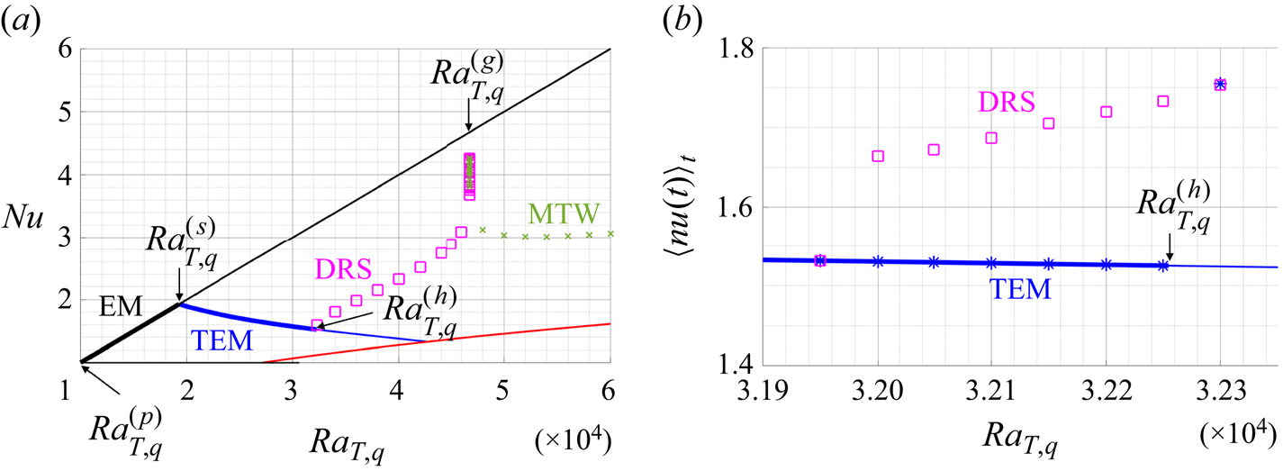
Figure 1 shows the resulting bifurcation diagram using thick (thin) lines for stable (unstable) states obtained from numerical continuation. The markers in figure 1 correspond to the final stable state as obtained from DNS. Figure 1(a) shows that the elevator mode (EM, black) bifurcates from the primary instability at $Ra_{T,q}^{(p)}=10^4$, consistent with (3.4), and that the Nusselt number of this mode displays a linear relation with $Ra_{T,q}$ according to (3.7). The secondary instability of the elevator mode at $Ra_{T,q}^{(s)}=19576.3$ leads to a branch of steady tilted elevator modes (TEMs, blue) accompanied by large-scale shear. Figure 2(a) shows the evolution of this shear from DNS at $Ra_{T,q}=3\times 10^4$, starting from an unstable elevator mode at this Rayleigh number. The figure shows that the large-scale shear $\langle u\rangle _h(z,t)$ becomes non-zero at $t\approx 2$ and then saturates in a horizontal flow with an approximately sinusoidal profile in the vertical. Figure 2(b) shows that the associated temperature deviation $T(x,z,t)$ at $t=10$ is tilted in the direction corresponding to the generated large-scale shear. This secondary bifurcation resembles the behaviour observed in RBC between fixed temperature boundaries, whereby a secondary bifurcation of steady convection rolls leads to tilted rolls accompanied by large-scale shear (Howard & Krishnamurti Reference Howard and Krishnamurti1986; Rucklidge & Matthews Reference Rucklidge and Matthews1996), as also observed in both experiments (Krishnamurti & Howard Reference Krishnamurti and Howard1981) and DNS (Matthews et al. Reference Matthews, Rucklidge, Weiss and Proctor1996; Goluskin et al. Reference Goluskin, Johnston, Flierl and Spiegel2014; Von Hardenberg et al. Reference Von Hardenberg, Goluskin, Provenzale and Spiegel2015; Wang et al. Reference Wang, Chong, Stevens, Verzicco and Lohse2020). This TEM branch terminates in another unstable steady state (red) that bifurcates from the conduction state without large-scale shear generation and resembles the two-layer (S2) solutions identified in salt-finger convection (Liu, Julien & Knobloch Reference Liu, Julien and Knobloch2022).

Figure 1.

(a) Bifurcation diagram with elevator mode (EM, black line), tilted elevator mode (TEM, blue line), direction-reversing state (DRS, magenta square) and modulated travelling waves (MTW, green cross). The bifurcation points include the primary bifurcation $Ra_{T,q}^{(p)}$, the secondary bifurcation $Ra_{T,q}^{(s)}$, the Hopf bifurcation $Ra_{T,q}^{(h)}$, and a global bifurcation at $Ra_{T,q}^{(g)}$. (b) Hysteresis diagram near the Hopf bifurcation point $Ra_{T,q}^{(h)}$ with TEM initial condition and increasing $Ra_{T,q}$ (blue star) or DRS initial conditions and decreasing $Ra_{T,q}$ (magenta square).

Figure 2.

(a) Large-scale shear $\langle u\rangle _h(z,t)$ and (b) temperature deviation $T(x,z,t)$ at $t=10$ for the steady TEM at $Ra_{T,q}=3\times 10^4$, $Pr=1$ and $L_x=0.2{\rm \pi}$.

The steady TEM loses stability at a Hopf bifurcation at $Ra_{T,q}^{(h)}=32085.1$ leading to oscillations about the TEM state with frequency $\omega _h=43.1$. This Hopf bifurcation is subcritical, however, implying that the tilted oscillations are unstable. Computations indicate that the system instead evolves into a symmetric direction-reversing state (DRS) with associated hysteresis near $Ra_{T,q}^{(h)}$ as shown in figure 1(b). Here, we use $\langle nu(t)\rangle _t$ to distinguish the TEM state from the DRS, reached from TEM initial conditions upon increasing $Ra_{T,q}$ (blue star) or from DRS initial conditions upon decreasing $Ra_{T,q}$ (magenta square). When $Ra_{T,q}< Ra_{T,q}^{(h)}$, the DNS with TEM initial conditions show excellent agreement with numerical continuation results (thick blue line), while DNS with TEM initial conditions at $Ra_{T,q}>Ra_{T,q}^{(h)}$ evolve into DRS. Figure 3 shows $\langle u \rangle _h(z,t)$ and $nu(t)$ at $Ra_{T,q}=32\,100$, a value slightly larger than $Ra_{T,q}^{(h)}$, with a TEM initial condition from a lower $Ra_{T,q}$. The large-scale flow oscillates with frequency $\omega \approx 43.0$ in $t\in [0,10]$ (not shown in figure 3) that is close to the Hopf frequency $\omega _h=43.1$ but does not reverse. At $t\approx 74$, the flow abruptly transitions to a DRS as shown in figure 3(a). Figure 3(b) shows the corresponding instantaneous Nusselt number $nu(t)$. Similar DRS are also observed in RBC (Sugiyama et al. Reference Sugiyama, Ni, Stevens, Chan, Zhou, Xi, Sun, Grossmann, Xia and Lohse2010; Chandra & Verma Reference Chandra and Verma2013; Winchester, Dallas & Howell Reference Winchester, Dallas and Howell2021), magnetoconvection (Matthews et al. Reference Matthews, Proctor, Rucklidge and Weiss1993; Proctor et al. Reference Proctor, Weiss, Brownjohn and Hurlburt1994) as well as in salt-finger convection (Liu et al. Reference Liu, Julien and Knobloch2022).

Figure 3.

(a) Large-scale shear $\langle u\rangle _{h}(z,t)$ and (b) instantaneous Nusselt number $nu(t)$ at $Ra_{T,q}=3.21\times 10^4$, $Pr=1$ and $L_x=0.2{\rm \pi}$ with a TEM initial condition (supplementary movie 1, available at https://doi.org/10.1017/jfm.2023.1057, shows the corresponding temperature deviation $T(x,z,t)$).

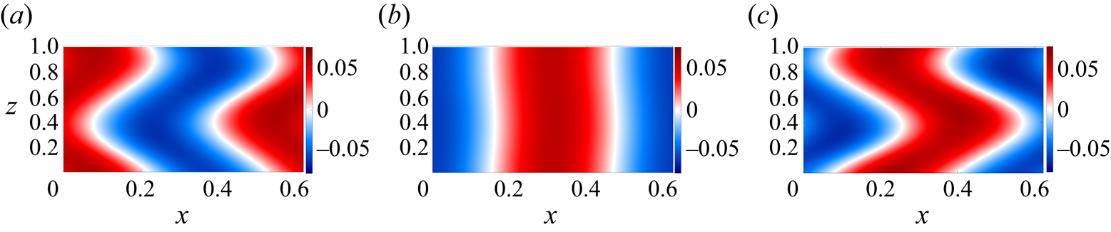
At higher Rayleigh numbers, this DRS spends more time displaying flow structures close to an elevator mode. Figure 4 shows three snapshots of the temperature deviation $T(x,z,t)$ at $Ra_{T,q}=4.6\times 10^4$. At $t=2.21$ and $t=2.37$, the temperature deviation tilts in opposite directions. At $t=2.29$, $T(x,z,t)$ displays flow structures close to an elevator mode, followed at $t=2.37$ by a restored and approximately reflected tilted state. At yet higher Rayleigh numbers, the DRS collides with the unstable steady elevator mode leading to a global bifurcation at $Ra_{T,q}^{(g)}\approx 46892.03$, as indicated in figure 1(a). At this global bifurcation, the DRS transitions to modulated travelling waves (MTW, green) that do not reverse direction. Figure 5(a) shows the corresponding large-scale shear $\langle u\rangle _h(z,t)$ at $Ra_{T,q}=6\times 10^4$. Figure 5(b) displays the corresponding temperature deviation $T(x,z,t)$ at $z=0.1$, including the MTW that sets in at $t\approx 0.8$. This global bifurcation is illustrated in the phase diagram shown in figure 6 near $Ra_{T,q}^{(g)}$, revealing an abrupt change in topology before and after this global bifurcation. Note that both states pass through $\langle T\rangle _h (z_p, t)=\langle u\rangle _h(z_p, t)=0$ corresponding to the elevator mode. A similar global bifurcation must take place on the subcritical DRS branch in order to generate the DRS from the oscillating TEM state, but is inaccessible to DNS. Such gluing bifurcations are also seen in RBC, where oscillatory tilted convection rolls originating from a Hopf bifurcation of steady tilted convection rolls may collide with steady convection rolls and glue together in a global bifurcation; see e.g. Rucklidge & Matthews (Reference Rucklidge and Matthews1996).

Figure 4.

Temperature deviation $T(x,z,t)$ associated with the DRS at three different times when $Ra_{T,q}=4.6\times 10^4$, $Pr=1$ and $L_x=0.2{\rm \pi}$: (a) $t=2.21$, (b) $t=2.29$, and (c) $t=2.37$.

Figure 5.

(a) Large-scale shear $\langle u\rangle _h(z,t)$ and (b) temperature deviation $T(x,z,t)$ at $z=0.1$ for MTWs at $Ra_{T,q}=6\times 10^4$, $Pr=1$ and $L_x=0.2{\rm \pi}$.

Figure 6.

Phase diagram showing $\langle T\rangle _h(z_p,t)$ as a function of $\langle u\rangle _h(z_p,t)$ at (a) $Ra_{T,q}=46\,892.0$ and(b) $Ra_{T,q}=46\,892.1$, with $z_p:={\text {arg\,max}}_{z} \langle T\rangle _h(z,t=10)$. The global bifurcation takes place in between.

3.4. Single-mode equations

The previous results show that the flow in the horizontal direction is dominated by a domain-filling mode. Moreover, in fixed-flux RBC, any long box will eventually contain a single pair of rolls (Chapman & Proctor Reference Chapman and Proctor1980), and domain-filling modes also organize the flow in the turbulent regime at high Rayleigh number (Vieweg et al. Reference Vieweg, Scheel and Schumacher2021, Reference Vieweg, Scheel, Stepanov and Schumacher2022; Käufer et al. Reference Käufer, Vieweg, Schumacher and Cierpka2023). This motivates us to derive single-mode equations that have been used successfully in a wide range of convection problems (Herring Reference Herring1963; Toomre, Gough & Spiegel Reference Toomre, Gough and Spiegel1977; Gough & Toomre Reference Gough and Toomre1982; Paparella & Spiegel Reference Paparella and Spiegel1999), especially for well-organized columnar structures in the presence of strong restraining body forces, including rapid rotation and strong magnetic field (Julien & Knobloch Reference Julien and Knobloch2007), or large-scale damping in salt-finger convection (Liu et al. Reference Liu, Julien and Knobloch2022), or convection in a porous medium (Liu & Knobloch Reference Liu and Knobloch2022).

Single-mode equations are obtained from a severely truncated Fourier expansion in the horizontal, which reduces the governing equations from three spatial dimensions to equations for the vertical solutions profile associated with a prescribed horizontal planform. Here, we derive the single-mode equations by decomposing variables into a mean mode in the horizontal and horizontal harmonics:

(3.8a)$$\begin{gather} T(x,y,z,t)=\bar{T}_0(z,t)+\hat{T}(z,t)\exp({\text{i}(k_x x+k_y y)})+\text{c.c.}, \end{gather}$$

(3.8b)$$\begin{gather}\boldsymbol{u}(x,y,z,t)=\bar{U}_0(z,t)\,\boldsymbol{e}_x+\hat{\boldsymbol{u}}(z,t) \exp({\text{i}(k_x x+k_y y)})+\text{c.c.}, \end{gather}$$

(3.8c)$$\begin{gather}p(x,y,z,t)=\bar{P}_0(z,t)+\hat{p}(z,t)\exp({\text{i}(k_x x+k_y y)})+\text{c.c.} \end{gather}$$

We truncate the resulting equations at these harmonics to obtain the single-mode equations:

(3.9a)$$\begin{gather} \partial_t \hat{u}+\bar{U}_0\text{i}k_x \hat{u}+\hat{w}\,\partial_z \bar{U}_0={-} \text{i}k_x \hat{p}+Pr\,\hat{\nabla}^2 \hat{u}, \end{gather}$$

(3.9b)$$\begin{gather}\partial_t \hat{v}+\bar{U}_0\text{i}k_x\hat{v}={-}\text{i}k_y \hat{p}+Pr\,\hat{\nabla}^2 \hat{v}, \end{gather}$$

(3.9c)$$\begin{gather}\partial_t \hat{w}+\bar{U}_0\text{i}k_x\hat{w}={-}\partial_z \hat{p}+Pr\,\hat{\nabla}^2\hat{w}+Pr\,Ra_{T,q}\,\hat{T}, \end{gather}$$

(3.9d)$$\begin{gather}\text{i}k_x \hat{u}+\text{i}k_y\hat{v}+\partial_z \hat{w}=0, \end{gather}$$

(3.9e)$$\begin{gather}\partial_t\hat{T}+\bar{U}_0\text{i}k_x\hat{T}+\hat{w}\,\partial_z \bar{T}_0- \hat{w}+\hat{w}\int_0^1\left(\hat{w}^* \hat{T}+\hat{w}\hat{T}^*\right){\rm d}z= \hat{\nabla}^2\hat{T}, \end{gather}$$

(3.9f)$$\begin{gather}\partial_t \bar{U}_0+\partial_z\left(\hat{w}^*\hat{u}+\hat{w}\hat{u}^*\right)= Pr\,\partial_z^2\bar{U}_0, \end{gather}$$

(3.9g)$$\begin{gather}\partial_t \bar{T}_0+\partial_z\left(\hat{w}^*\hat{T}+\hat{w}\hat{T}^*\right)= \partial_z^2 \bar{T}_0. \end{gather}$$

Here, the integral term in (3.9e) represents the fixed-flux constraint originating from $w\langle wT\rangle _{h,v}$ in (2.7c). The horizontal wavenumber is chosen as $k_x=10$ and $k_y=0$ corresponding to a domain-filling mode within a 2-D domain with $L_x=0.2{\rm \pi}$. Numerical continuation of the single-mode equations (3.9) is performed using pde2path (Uecker et al. Reference Uecker, Wetzel and Rademacher2014; Uecker Reference Uecker2021a) with $N_z=128$, while DNS of (3.9) are conducted using Dedalus (Burns et al. Reference Burns, Vasil, Oishi, Lecoanet and Brown2020) with $N_z=128$.

Figure 7(a) shows the bifurcation diagram, while figure 7(b) shows the hysteresis diagram obtained from the single-mode equations in (3.9). Here, we can see that the single-mode equations reproduce the bifurcation and hysteresis diagrams obtained from the full equations in two dimensions, shown in figure 1. The hysteresis behaviour in figure 7(b) is present in a similar Rayleigh number range, $\Delta Ra_{T,q}\approx 200$, as in figure 1(b). Nevertheless, the bifurcation points are shifted slightly in the single-mode equations compared with the full equations, as shown in table 1. The success of the single-mode equations in predicting the Hopf frequency is perhaps in the same spirit as the real zero imaginary frequency (RZIF) ansatz that has shown success in predicting the oscillation frequency in nonlinear thermosolutal convection and shear flow (Turton, Tuckerman & Barkley Reference Turton, Tuckerman and Barkley2015; Bengana et al. Reference Bengana, Loiseau, Robinet and Tuckerman2019; Bengana & Tuckerman Reference Bengana and Tuckerman2021). Within the RZIF framework, the eigenvalues are computed based on dynamics linearized around a mean flow that can deviate from the laminar base flow, much as here the single-mode equations employ the large-scale modes $\bar {T}_0$ and $\bar {U}_0$ with superposed harmonics; see (3.9f) and (3.9g).

Figure 7.

Same as figure 1 but obtained from the single-mode equations in (3.9).

Table 1.

Comparison of the bifurcation points between the full 2-D equations in (2.7) with $L_x=0.2{\rm \pi}$, and the single-mode equations in (3.9) with $k_x=10$, including the primary bifurcation $Ra_{T,q}^{(p)}$, the secondary bifurcation $Ra_{T,q}^{(s)}$, the Hopf bifurcation $Ra_{T,q}^{(h)}$ with Hopf frequency $\omega _h$, and the global bifurcation $Ra_{T,q}^{(g)}$, all at $Pr=1$.

We further leverage the computational efficiency of single-mode equations to analyse the frequency scaling near the global bifurcation. We perform a bisection over $Ra_{T,q}$ using DNS of the single-mode equations in (3.9) to identify the global bifurcation point with more significant digits, $Ra_{T,q}^{(g)}=46\,761.0819762429$, than possible from the full equations. Figure 8 shows that the period $T_p$ of the direction reversals near $Ra_{T,q}^{(g)}$ diverges as $T_p=-0.0448\ln (Ra_{T,q}^{(g)}-Ra_{T,q})+0.6118$; cf. Knobloch & Proctor (Reference Knobloch and Proctor1981) and Knobloch (Reference Knobloch1986).

Figure 8.

(a) The reversal period $T_p$ as a function of $Ra_{T,q}$ near the global bifurcation $Ra_{T,q}^{(g)}$ obtained from the single-mode equations in (3.9) at $Pr=1$ and $k_x=10$. The black dashed line is $T_p=-0.0448\ln (Ra_{T,q}^{(g)}-Ra_{T,q})+0.6118$ and fits the DNS data with a relative residue of $0.4\,\%$, where $Ra_{T,q}^{(g)}=46\,761.0819762429$. (b) The leading eigenvalues of the (unstable) elevator mode at $Ra_{T,q}^{(g)}$ within the single-mode equations (3.9).

Since the DRS collides with an unstable elevator mode at the global bifurcation $Ra_{T,q}^{(g)}$, as indicated in figure 7(a), it is instructive to compute the eigenvalues of the elevator mode at this point within the single-mode equations (3.9). Figure 8(b) shows that the unstable eigenvalue $\lambda _1=43.69$ is real, and that the least stable eigenvalues are complex, with $\lambda _{2,3}=-\rho \pm \text {i}\omega =-49.27 \pm \text {i}117.11$. Thus this global bifurcation is associated with a saddle-focus equilibrium with $\delta \equiv \rho /\lambda _1=1.13>1$, i.e. the tame version of the Shilnikov bifurcation (Shilnikov Reference Shilnikov1965; Shilnikov & Shilnikov Reference Shilnikov and Shilnikov2007). Here, we report these eigenvalues from the single-mode equations (3.9) to facilitate direct comparison of the logarithmic scaling law in figure 8(a) with theory. For the 2-D full equations, the corresponding eigenvalues of the elevator mode at the corresponding $Ra_{T,q}^{(g)}$ are $\lambda _1=41.11$, $\lambda _{2,3}=-\rho \pm \text {i}\omega =-56.67\pm \text {i}114.67$, leading to a Shilnikov bifurcation with $\delta =1.38$.

The logarithmic scaling law and associated coefficient can be predicted by constructing a Poincaré map near the global bifurcation point $Ra_{T,q}^{(g)}$ and the saddle-focus equilibrium (here the steady elevator mode) by composing a local map near this saddle focus and a global map (Shilnikov & Shilnikov Reference Shilnikov and Shilnikov2007), as done by Glendinning & Sparrow (Reference Glendinning and Sparrow1984). For the local map, we consider the flow linearized around this elevator mode with $\mu :=Ra_{T,q}^{(g)}-Ra_{T,q}\ll 1$:

(3.10a)$$\begin{gather} \dot{\zeta}=\lambda_1 \zeta +\text{h.o.t.}, \end{gather}$$

(3.10b)$$\begin{gather}\dot{\theta}=\omega+\text{h.o.t.}, \end{gather}$$

(3.10c)$$\begin{gather}\dot{r}={-}\rho r +\text{h.o.t.}, \end{gather}$$

where $\zeta$ is the coordinate corresponding to the unstable eigenvalue, $(r,\theta )$ are the polar coordinates associated with the least stable eigenvalues, and h.o.t. refers to higher-order terms. We consider the Poincaré section $\varSigma ^{in}:=\{\theta =0\}$ and $\varSigma ^{out}:=\{\zeta =H\}$, and construct the local map $\varPi _{loc}:\varSigma ^{in}\rightarrow \varSigma ^{out}$ according to the linearized dynamics in (3.10):

(3.11a)$$\begin{gather} H=\zeta(T_f)=\zeta_0\,{\rm e}^{\lambda_1 T_f}, \end{gather}$$

(3.11b)$$\begin{gather}r(T_f)=r_0\,{\rm e}^{-\rho T_f}, \end{gather}$$

(3.11c)$$\begin{gather}\theta(T_f)=\omega T_f. \end{gather}$$

From (3.11a), the time of flight $\varSigma ^{in}:=\{\theta =0\}\to \varSigma ^{out}:=\{\zeta =H\}$ is

(3.12)\begin{equation} T_f={-}\frac{1}{\lambda_1}\ln \left( \frac{\zeta_0}{H}\right). \end{equation}

Substituting (3.12) into (3.11), we obtain the local map:

(3.13) \begin{equation} \varPi_{loc}:(r,\theta,\zeta)\rightarrow \biggl( r_0\left(\frac{\zeta_0}{H} \right)^{\delta},\frac{\omega}{\lambda_1}\ln\left(\frac{H}{\zeta_0}\right),H \biggr). \end{equation}

The global map $\varPi _{global}:\varSigma ^{out}\rightarrow \varSigma ^{in}$ is obtained from a Taylor series around the homoclinic orbit assumed to be present at $\mu =0$:

(3.14) \begin{align} \varPi_{global}: (r,\theta,h)\rightarrow (\bar{r}+a\mu+br\cos \theta +cr\sin\theta,0,d\mu+er\cos\theta+fr\sin\theta)+\text{h.o.t.}, \end{align}

where $a$, $b$, $c$, $d$, $e$ and $f$ are constants. By composing the local and global maps ($\varPi :\varSigma ^{in}\rightarrow \varSigma ^{in}=\varPi _{global}\circ \varPi _{loc}$), we obtain the Poincaré map

(3.15)\begin{equation} \varPi: \begin{bmatrix} r\\ \zeta \end{bmatrix}\rightarrow \begin{bmatrix} \bar{r}\\ 0 \end{bmatrix}+\begin{bmatrix} a\\ d \end{bmatrix}\mu+\begin{bmatrix} c_1 r \zeta^{\delta}\cos(k_1 \ln \zeta +\phi_1)\\ c_2 r \zeta^{\delta} \cos(k_2 \ln \zeta +\phi_2) \end{bmatrix}+\text{h.o.t.}, \end{equation}

where $c_i$, $k_i$ and $\phi _i$ ($i=1,2$) are constants. We may now search for a fixed point of the Poincaré map $\varPi$ that corresponds to the periodic orbit near $Ra_{T,q}^{(g)}$ in the original system. This point is approximated by the fixed point of the one-dimensional map

(3.16)\begin{equation} \zeta-d \mu=\varPhi(\zeta)\equiv c_2 r \zeta^{\delta}\cos(k_2\ln \zeta +\phi_2)+\text{h.o.t.} \end{equation}

When $\delta >1$, there is a unique fixed point of (3.16), which scales as $\zeta \sim d\mu$ near the global bifurcation $\mu \rightarrow 0$. Thus based on (3.12) and the assumption that the global return is much faster than the local passage past the fixed point, the period of the reversing orbit just before the global bifurcation scales as

(3.17)\begin{equation} T_p={-}\frac{2}{\lambda_1} \ln \mu +\text{const.}={-}\frac{2}{\lambda_1}\ln \left(Ra_{T,q}^{(g)}-Ra_{T,q}\right)+\text{const}. \end{equation}

Here, the factor 2 arises because the orbit makes two passes near the fixed point in each reversal period. Using $\lambda _1$ from figure 8(b), this calculation predicts that $2/\lambda _1=0.04578$, a coefficient that is almost exactly that obtained from the fit to the simulation data in figure 8(a).

4. Dynamics at high Rayleigh numbers

In this section, we study the dynamics at higher Rayleigh numbers, where chaotic behaviour appears. We first analyse the secondary instability of the elevator mode, which continues to play an important role in the high Rayleigh number regime. We focus on the 2-D elevator mode with a horizontal wavenumber $k_x=k_e$ in the $x$ direction,

(4.1a,b)\begin{equation} \bar{W}_e(x)=\hat{w}_e \exp(\text{i}k_e x)+{\rm c.c}.,\quad \bar{T}_e(x)=\hat{T}_e\exp(\text{i}k_e x)+{\rm c.c}., \end{equation}

and solution amplitude given by (3.6a,b). The decomposition

(4.2a,b)\begin{equation} \boldsymbol{u}=\bar{W}_e\boldsymbol{e}_z+\boldsymbol{u}',\quad T=\bar{T}_e+T' \end{equation}

leads to the linearized equations

(4.3a)$$\begin{gather} \frac{\partial \boldsymbol{u}'}{\partial t}+u'\,\frac{{\rm d}\bar{W}_e}{{\rm d}\kern 0.06em x}\, \boldsymbol{e}_z+\bar{W}_e\,\partial_z \boldsymbol{u}'={-}\boldsymbol{\nabla}p'+Pr\,Ra_{T,q}\,T'\boldsymbol{e}_z+Pr\, \nabla^2 \boldsymbol{u}', \end{gather}$$

(4.3b)$$\begin{gather}\boldsymbol{\nabla}\boldsymbol{\cdot} \boldsymbol{u}'=0, \end{gather}$$

(4.3c)$$\begin{gather}\frac{\partial T'}{\partial t}+u'\,\frac{{\rm d}\bar{T}_e}{{\rm d}\kern 0.06em x}+ \bar{W}_e\,\partial_z T'-w'+w'\langle \bar{W}_e\bar{T}_e\rangle_{h,v}=\nabla^2T'. \end{gather}$$

The cubic flux-feedback nonlinearity $w\langle wT\rangle _{h,v}$ in (2.7c) generates three linearized terms:

(4.4)\begin{equation} w'\langle \bar{W}_e\bar{T}_e\rangle_{h,v}+\bar{W}_e\langle w'\bar{T}_e\rangle_{h,v}+\bar{W}_e\langle \bar{W}_eT'\rangle_{h,v}, \end{equation}

with the latter two terms in (4.4) vanishing for $k_z\neq 0$. As a result, only the term $w'\langle \bar {W}_e\bar {T}_e\rangle _{h,v}$ originating from flux feedback appears in the linearized equation in (4.3c). The normal mode assumption in general 3-D form

(4.5a)$$\begin{gather} \boldsymbol{u}'=\tilde{\boldsymbol{u}}(x) \exp[\text{i}(k_y y+k_z z)+\lambda t]+\text{c.c.}, \end{gather}$$

(4.5b)$$\begin{gather}T'=\tilde{T}(x)\exp[\text{i}(k_y y+k_z z)+\lambda t]+\text{c.c.} \end{gather}$$

contains the coefficients $\tilde {\boldsymbol {u}}(x)$ and $\tilde {T}(x)$ that depend on $x$ because the base flow (elevator mode) also depends on $x$. In terms of the horizontal vorticity $\tilde {\omega }_x:=\text {i}k_y \tilde {w}-\text {i}k_z\tilde {v}$, we have the linear eigenvalue problem

(4.6)\begin{equation} \lambda \begin{bmatrix} \tilde{u}\\ \tilde{\omega}_x\\ \tilde{T} \end{bmatrix} = \begin{bmatrix} \mathcal{A}_{11} & \mathcal{A}_{12} & \mathcal{A}_{13}\\ \mathcal{A}_{21} & \mathcal{A}_{22} & \mathcal{A}_{23} \\ \mathcal{A}_{31} & \mathcal{A}_{32} & \mathcal{A}_{33} \end{bmatrix} \begin{bmatrix} \tilde{u}\\ \tilde{\omega}_x\\ \tilde{T} \end{bmatrix}=:\mathcal{A}\begin{bmatrix} \tilde{u}\\ \tilde{\omega}_x\\ \tilde{T} \end{bmatrix}, \end{equation}

where

(4.7a)$$\begin{gather} \mathcal{A}_{11}=\tilde{\nabla}^{{-}2}\left(-\text{i}k_z \bar{W}_e\,\tilde{\nabla}^2+ \text{i}k_z\,\frac{{\rm d}^2\bar{W}_e}{{{\rm d}\kern 0.06em x}^2}+Pr\,\tilde{\nabla}^4\right), \end{gather}$$

(4.7b)$$\begin{gather}\mathcal{A}_{12}=0, \end{gather}$$

(4.7c)$$\begin{gather}\mathcal{A}_{13}=\tilde{\nabla}^{{-}2}\,Pr\,Ra_{T,q}\,(-\text{i}k_z\,\partial_x), \end{gather}$$

(4.7d)$$\begin{gather}\mathcal{A}_{21}={-}\text{i}k_y\,\frac{{\rm d}\bar{W}_e}{{\rm d}\kern 0.06em x}, \end{gather}$$

(4.7e)$$\begin{gather}\mathcal{A}_{22}={-}\text{i}k_z \bar{W}_e+Pr\,\tilde{\nabla}^2, \end{gather}$$

(4.7f)$$\begin{gather}\mathcal{A}_{23}=Pr\,Ra_{T,q}\,\text{i}k_y, \end{gather}$$

(4.7g)$$\begin{gather}\mathcal{A}_{31}={-}\frac{{\rm d}\bar{T}_e}{{\rm d}\kern 0.06em x}+[1-\langle \bar{W}_e\bar{T}_e \rangle_{h,v}]\,\frac{\text{i}k_z\,\partial_x }{k_y^2+k_z^2}, \end{gather}$$

(4.7h)$$\begin{gather}\mathcal{A}_{32}=[1-\langle \bar{W}_e\bar{T}_e\rangle_{h,v}]\, \frac{-\text{i}k_y}{k_y^2+k_z^2}, \end{gather}$$

(4.7i)$$\begin{gather}\mathcal{A}_{33}={-}\text{i}k_z \bar{W}_e+\tilde{\nabla}^2, \end{gather}$$

with $\tilde {\nabla }^2:=\partial _x^2-k_y^2-k_z^2$, and $\tilde {\nabla }^4:=\partial _x^4-2(k_y^2+k_z^2)\,\partial _x^2+(k_y^2+k_z^2)^2$.

We compare the above formulation with that without the flux feedback, corresponding to setting the integral flux-feedback terms $\langle \bar {W}_e\bar {T}_e\rangle _{h,v}$ in (4.7g)–(4.7h) to zero, leading to a modified eigenvalue problem with $\mathcal {A}$ in (4.6) replaced by

(4.8)\begin{equation} \underline{\mathcal{A}}:=\begin{bmatrix} \mathcal{A}_{11} & \mathcal{A}_{12} & \mathcal{A}_{13}\\ \mathcal{A}_{21} & \mathcal{A}_{22} & \mathcal{A}_{23}\\ \underline{\mathcal{A}}_{31} & \underline{\mathcal{A}}_{32} & \mathcal{A}_{33} \end{bmatrix}, \end{equation}

where

(4.9a,b)\begin{equation} \underline{\mathcal{A}}_{31}:={-}\frac{{\rm d}\bar{T}_e}{{\rm d}\kern 0.06em x}+\frac{\text{i}k_z\, \partial_x }{k_y^2+k_z^2},\quad \underline{\mathcal{A}}_{32}:=\frac{-\text{i}k_y}{k_y^2+k_z^2}. \end{equation}

The horizontal direction is discretized using a Fourier collocation method with the horizontal derivative computed using a Fourier differentiation matrix (Weideman & Reddy Reference Weideman and Reddy2000). The numerical implementation is validated against Floquet-based linear stability analysis (Holyer Reference Holyer1984; Garaud, Gallet & Bischoff Reference Garaud, Gallet and Bischoff2015; Radko Reference Radko2016; Garaud, Kumar & Sridhar Reference Garaud, Kumar and Sridhar2019). We choose the horizontal domain $L_x$ to contain one or more wavelengths of the elevator wavelength $2{\rm \pi} /k_e$. For all the results reported here, we take $k_y=0$ corresponding to a 2-D configuration.

Figure 9(a) shows the growth rate $\max [{\rm Re}(\lambda )]$, comparing the fixed-flux case computed from $\mathcal {A}$ in (4.6) with the case without flux feedback computed from $\underline {\mathcal {A}}$ in (4.8). The flux feedback leads to $\lambda =0$ at $k_z=0$, and the instability is limited to a small range of $k_z$, a feature observed widely in systems with a conservation law (Matthews & Cox Reference Matthews and Cox2000). For the case without flux feedback, its growth rate is larger and decays to zero only at much higher wavenumbers $k_z$ (not shown in figure 9a). We further identify the wavenumbers $k_{z,0}$ and $k_{z,max}$ indicated in figure 9(a) corresponding, respectively, to zero growth rate and maximum growth rate:

(4.10a)$$\begin{gather} \lambda(k_{z,0})=0\quad \text{with } k_{z,0}\neq 0, \end{gather}$$

(4.10b)$$\begin{gather}k_{z,max}:=\underset{k_z}{\text{arg\,max}} \,{\rm Re}(\lambda). \end{gather}$$

Figure 9(b) displays $k_{z,0}$ and $k_{z,max}$, both of which increase as $Ra_{T,q}$ increases, with $k_{z,max}< k_{z,0}$. Here, we also plot $k_{z}=2{\rm \pi}$, which is the smallest non-trivial vertical wavenumber that fits in the $L_z=1$ domain. The secondary instability wavelength is not required to lie within $L_z=1$, thus a comparison of $k_{z,0}$ with $k_z=2{\rm \pi}$ determines whether the secondary instability can occur within the domain, or whether it is suppressed by its finite size. Figure 9(b) shows that $k_{z,0}>2{\rm \pi}$ when $L_x=0.2{\rm \pi}$ and $Ra_{T,q}\geq 3\times 10^4$, a result consistent with the presence of a secondary instability in an $L_z=1$ domain identified in § 3.

Figure 9.

(a) The growth rate $\max [{\rm Re}(\lambda )]$ at $Ra_{T,q}=10^8$, $Pr=1$, $L_x=0.2{\rm \pi}$ and $k_e=10$, with flux feedback computed from $\mathcal {A}$ in (4.6), and without flux feedback as computed from $\underline {\mathcal {A}}$ in (4.8). (b) The wavenumbers $k_{z,0}$ and $k_{z,max}$ as functions of $Ra_{T,q}$ at $Pr=1$, $L_x=0.2{\rm \pi}$ and $k_e=10$. The red dashed line corresponds to $k_z=2{\rm \pi}$.

The secondary instability of the elevator mode and the MTWs generated through the sequence of bifurcations examined in § 3 continue to play an important role at larger Rayleigh numbers. Figure 10 displays DNS results at $Ra_{T,q}=10^8$ obtained with $N_x=N_z=256$ grid points ($N_x=N_z=512$ grid points generate the same behaviour). The large-scale shear $\langle u\rangle _{h}(z,t)$ in figure 10(a) is now dominated by MTWs, but displays chaotic behaviour. In addition, it slowly migrates in the vertical direction, behaviour that is permitted by the periodic boundary conditions in the vertical.

Figure 10.

(a) Large-scale shear $\langle u\rangle _h(z,t)$, (b) total temperature $1+ \bar {\mathcal {T}}_{z,q} z+\langle T\rangle _{h,t}(z)$ (solid black line) compared with the linear profile $1+ \bar {\mathcal {T}}_{z,q} z$ (dashed blue line), and (c) root mean square vertical velocity $\sqrt {\langle ww\rangle _{h,t}}$, the latter two averaged over $t\in [0.275,0.465]$, at $Ra_{T,q}=10^8$, $Pr=1$ and $L_x=0.2{\rm \pi}$.

The mean total temperature averaged over $t\in [0.275,0.465]$ in figure 10(b) exhibits a deviation from a linear profile similar to canonical RBC. Moreover, in the region where the mean temperature deviation $\langle T\rangle _{h,t}(z)$ is close to zero, the corresponding large-scale shear $\langle u\rangle _{h}(z,t)$ also vanishes (white regions in figure 10a) and the root mean square (r.m.s.) vertical velocity $\sqrt {\langle ww\rangle _{h,t}}$ displays local minima with a zero vertical derivative, as shown in figure 10(c). The local maxima of the r.m.s. vertical velocity $\sqrt {\langle ww\rangle _{h,t}}$ correspond instead to the mixed mean temperature regions in figure 10(b). This behaviour resembles that of RBC in a bounded domain with constant temperature boundaries and no-slip instead of stress-free velocity boundary conditions at the top and bottom (van der Poel et al. Reference van der Poel, Ostilla-Mónico, Verzicco and Lohse2014). The figure shows that the fixed-flux constraint suppresses bursting behaviour compared with homogeneous RBC driven by a constant temperature gradient (Borue & Orszag Reference Borue and Orszag1997; Lohse & Toschi Reference Lohse and Toschi2003; Calzavarini et al. Reference Calzavarini, Lohse, Toschi and Tripiccione2005, Reference Calzavarini, Doering, Gibbon, Lohse, Tanabe and Toschi2006). Figure 11 shows the Nusselt number scaling within $Ra_{T,q}\in [10^8,10^{10}]$ computed with $N_x=N_z=512$ grid points and $L_x=0.2{\rm \pi}$, $Pr=1$. Here, the fitted scaling law $Nu=0.189\,Ra_{T,q}^{0.217}$ is associated with an exponent lower than $Nu\sim Ra_{T,q}^{1/3}$ corresponding to ultimate regime scaling $Nu\sim Ra_T^{1/2}$. However, the flow structures associated with figure 11 are dominated by large-scale shear with a $\langle u\rangle _h(z,t)$ profile similar to that in figure 10(a), potentially reducing heat transport.

Figure 11.

Plot of $Nu$ as a function of $Ra_{T,q}$ from DNS with $L_x=0.2{\rm \pi}$ and $Pr=1$.

The impact of the domain size and of the horizontal wavenumber of the elevator mode within the domain is analysed further in figure 12(a), which shows $k_{z,0}$ and $k_{z,max}$ as functions of $L_x$ when $k_e=2{\rm \pi} /L_x$, $Ra_{T,q}=10^8$ and $Pr=1$. As the horizontal domain and wavelength increase, both $k_{z,0}$ and $k_{z,max}$ decrease, suggesting a small vertical wavenumber of the secondary instability. With $L_z$ fixed at $L_z=1$, this requires that we choose a small enough horizontal domain such that $k_{z,0}\geq 2{\rm \pi}$. A similar requirement applies for mean flow generation in canonical RBC (Rucklidge & Matthews Reference Rucklidge and Matthews1996; Fitzgerald & Farrell Reference Fitzgerald and Farrell2014; Wang et al. Reference Wang, Chong, Stevens, Verzicco and Lohse2020) and is the reason for choosing $L_x=0.2{\rm \pi}$ for most of the results in this paper. Figure 12(b) then fixes $L_x$ at $L_x=0.4{\rm \pi}$, but varies $k_e$, allowing multiple elevator modes within the domain. Evidently, both $k_{z,0}$ and $k_{z,max}$ increase as $k_e$ increases, and both are fitted well by a linear scaling law. This trend can be confirmed also in DNS. The associated large-scale shear $\langle u\rangle _h(z,t)$ in figure 13(a) shows that $k_z=4{\rm \pi}$ for an initial elevator mode wavenumber $k_e=20$, while $\langle u\rangle _h(z,t)$ in figure 13(b) displays a $k_z=6{\rm \pi}$ instability associated with $k_e=30$. This observation corresponds directly to the $k_{z,max}$ value at $k_e=20$ and $30$ predicted by the secondary instability analysis in figure 12(b).

Figure 12.

The wavenumbers $k_{z,0}$ and $k_{z,max}$ as functions of (a) $L_{x}$ when $k_e=2{\rm \pi} /L_x$, and (b) $k_e$ with $L_x=0.4{\rm \pi}$. The linear fit is $k_{z,0}=0.98k_e+0.10$ (black dash-dotted line) and $k_{z,max}=0.57k_e+0.20$ (blue dash-dotted line). The dashed red lines indicate $k_z=2{\rm \pi}$. Instability requires that $k_{z,0}>2{\rm \pi}$. Other parameters are $Ra_{T,q}=10^8$ and $Pr=1$.

Figure 13.

Large-scale shear $\langle u\rangle _h(z,t)$ with initial elevator mode wavenumber (a) $k_e=20$ and (b) $k_e=30$, both at $Ra_{T,q}=10^8$, $Pr=1$ and $L_x=0.4{\rm \pi}$.

In a domain of horizontal size $L_x=0.4{\rm \pi}$, the final state is a stable domain-filling elevator mode with $k_e=5$ corresponding to the white region in figure 13 at $Ra_{T,q}=10^8$. A similar transition to a larger horizontal scale is also observed in fixed-flux RBC within both the weakly nonlinear regime (Chapman & Proctor Reference Chapman and Proctor1980) and the turbulent regime (Vieweg et al. Reference Vieweg, Scheel and Schumacher2021, Reference Vieweg, Scheel, Stepanov and Schumacher2022; Käufer et al. Reference Käufer, Vieweg, Schumacher and Cierpka2023). The stable elevator mode that results suggests that vertical jets (i.e. elevator modes) are favoured in wide domains, while horizontal jets are found in narrow domains. This behaviour resembles that in rapidly rotating convection where jets parallel to the short side of an anisotropic domain are found (Julien, Knobloch & Plumley Reference Julien, Knobloch and Plumley2018), or in 2-D turbulence driven by stochastic forcing (Bouchet & Simonnet Reference Bouchet and Simonnet2009). At higher Rayleigh numbers, the flow in wider domains does become turbulent despite the absence of a shear-generating instability. For example, when $L_x=0.4{\rm \pi}$, this instability is absent since $k_{z,0}<2{\rm \pi}$. However, when the Rayleigh number is increased to $Ra_{T,q}=10^{10}$, the flow nonetheless becomes turbulent or at least chaotic. Figure 14 shows two snapshots of a solution with $N_x=N_z=512$ grid points at these parameter values, displaying intermittent layering and vortex dipole generation. The mechanism responsible for destabilizing the stationary elevator state at these large Rayleigh numbers remains to be studied.

Figure 14.

Snapshots of the temperature deviation $T(x,z,t)$ at (a) $t=0.03$ and (b) $t=0.032$. Parameters are $Ra_{T,q}=10^{10}$, $L_x=0.4{\rm \pi}$ and $Pr=1$.

5. Prandtl number effect

In this section, we investigate the effect of the Prandtl number using the full 2-D equations. A low Prandtl number is of interest in astrophysical applications, where the heat transport is dominated by photon diffusion (Garaud Reference Garaud2018, Reference Garaud2021). Prandtl number $Pr=7$ corresponds to thermal diffusivity in water appropriate to oceanographic applications. When the temperature field is exchanged for a concentration such as salinity, the corresponding thermal diffusivity is replaced by molecular diffusivity, leading to Prandtl numbers as large as $Pr=700$.

Figure 15 shows a bifurcation diagram similar to figure 1(a) but with ${Pr=0.1}$ and $Pr=7$ in figures 15(a,b), respectively. The onset of the primary instability $Ra_{T,q}^{(p)}$ and the amplitude of the resulting elevator mode branch are not affected by $Pr$, consistent with the analytical results in § 3.1. At low Prandtl numbers, the secondary bifurcation point $Ra_{T,q}^{(s)}$ and the Hopf bifurcation point $Ra_{T,q}^{(h)}$ are both shifted to much lower Rayleigh numbers, while increasing $Pr$ shifts these bifurcation points to a higher Rayleigh number. These bifurcation points and the associated Hopf frequency $\omega _h$ are listed in table 2. The Hopf frequency in table 2 obtained from numerical continuation is also very close to the oscillation frequency obtained from DNS at a parameter close to $Ra_{T,q}^{(h)}$ (not shown). Table 2 compares the bifurcation points computed from the full 2-D equations in (2.7) with the corresponding results from the single-mode equations in (3.9). The latter are in closer agreement with the full 2-D equations at ${Pr=0.1}$ than at $Pr=7$ because a low Prandtl number shifts these bifurcation points closer to the onset of primary instability at $Ra_{T,q}^{(p)}$. A related phenomenon is found in RBC, where at low $Pr$, a steady convection roll becomes immediately unstable to a large-scale (zonal) mode (Winchester, Howell & Dallas Reference Winchester, Howell and Dallas2022). The orange markers in figure 15 show the Nusselt number of the time-dependent states obtained from DNS, where the low Prandtl number case follows closely that of the TEM branch.

Figure 15.

Bifurcation diagram with an elevator mode (EM, black line), tilted elevator mode (TEM, blue) and time-dependent states (orange circles) at (a) ${Pr=0.1}$ and (b) $Pr=7$. The bifurcation points include the primary bifurcation $Ra_{T,q}^{(p)}$, the secondary bifurcation $Ra_{T,q}^{(s)}$, and a Hopf bifurcation $Ra_{T,q}^{(h)}$. The horizontal domain size is $L_x=0.2{\rm \pi}$.

Table 2.

Comparison of bifurcation points between the full 2-D equations in (2.7) with $L_x=0.2{\rm \pi}$, and the single-mode equations in (3.9) with $k_x=10$, including the primary bifurcation $Ra_{T,q}^{(p)}$, the secondary bifurcation $Ra_{T,q}^{(s)}$, the Hopf bifurcation $Ra_{T,q}^{(h)}$, and the Hopf frequency $\omega _h$ at ${Pr=0.1}$ and $Pr=7$.

Figure 16(a) displays the large-scale shear $\langle u\rangle _h(z,t)$ found at $Ra_{T,q}=10\,800$ and ${Pr=0.1}$. The instantaneous Nusselt number grows exponentially from $Nu\approx 1$ corresponding to the conduction state, and saturates at $Nu\approx 1.08$ associated with the elevator mode based on (3.7). The Nusselt number then decreases rapidly to $Nu\approx 1$ as a result of shear generation. Four different snapshots corresponding to the four different markers in figure 16(b) are shown in figure 17. Here, the elevator mode grows from $t=160$ to $t=166$ and then tilts at $t=166.5$, followed by rapid decay back towards the conduction state at $t=167$. This behaviour resembles a relaxation oscillation between the conduction base state and the steady elevator mode associated with different time scales between the growth and decay of the elevator mode. A similar oscillation cycle between a sheared state and convection rolls is also observed in RBC (Matthews et al. Reference Matthews, Rucklidge, Weiss and Proctor1996; Goluskin et al. Reference Goluskin, Johnston, Flierl and Spiegel2014) and magnetoconvection (Matthews, Proctor & Weiss Reference Matthews, Proctor and Weiss1995). More generally, relaxation oscillations associated with disparate time scales are also observed widely in binary fluid convection (Batiste et al. Reference Batiste, Knobloch, Alonso and Mercader2006), double-diffusive convection (Beaume, Bergeon & Knobloch Reference Beaume, Bergeon and Knobloch2018) and convection in a rapidly rotating sphere (Busse Reference Busse2002). Burst behaviour similar to the relaxation oscillation cycle observed here can be described by a 2-D ordinary differential equation model, where a burst is triggered by a symmetry-breaking instability of a growing symmetric state when it reaches a certain amplitude (Batiste et al. Reference Batiste, Knobloch, Mercader and Net2001; Bergeon & Knobloch Reference Bergeon and Knobloch2002). The prevalence of large-scale shear at low $Pr$ is known to lead to suppression of convection, an effect observed widely in the low-$Pr$ regime of RBC; see e.g. Schumacher & Sreenivasan (Reference Schumacher and Sreenivasan2020, figure 9). The suppression of convection by large-scale shear resembles the suppression of turbulence by self-generated mean flows (Shats et al. Reference Shats, Xia, Punzmann and Falkovich2007).

Figure 16.

(a) Large-scale shear $\langle u\rangle _{h}(z,t)$ and (b) instantaneous Nusselt number $nu(t)$ displaying relaxation oscillations at $Ra_{T,q}=10\,800$, ${Pr=0.1}$ and $L_x=0.2{\rm \pi}$.

Figure 17.

Evolution of the temperature deviation $T(x,z,t)$ during a burst corresponding to the four times indicated in figure 16(b): (a) $t=160$ (black star), (b) $t=166$ (blue circle), (c) $t=166.5$ (magenta square), and (d) $t=167$ (red cross). Parameters are $Ra_{T,q}=10\,800$, ${Pr=0.1}$ and $L_x=0.2{\rm \pi}$ (see supplementary movie 2).

Figure 18(a) shows $nu(t)$ at a higher Rayleigh number, $Ra_{T,q}=11\,900$. This time series no longer displays visible periodic behaviour, but its power spectrum density in figure 18(b) shows multiple peaks corresponding to frequencies $m\,f_1+n\,f_2$ with $f_1=0.1483$, $f_2=0.2044$ and $m,n\in \mathbb {Z}^+$. We conclude that the state in figure 18(a) is quasi-periodic, and likely generated by a torus bifurcation (equivalently, a Hopf bifurcation of a periodic orbit). Quasi-periodic orbits are also observed prior to the onset of non-periodic motion in RBC (Ahlers & Behringer Reference Ahlers and Behringer1978; Yahata Reference Yahata1982). At yet higher Rayleigh numbers, chaotic behaviour appears as shown in figure 19 for $Ra_{T,q}=13\,000$. The broad power spectrum density (PSD) is indicative of a chaotic state. The instantaneous Nusselt number does not reach the amplitude corresponding to the saturated steady elevator mode with $Nu=1.3$, as shown in figure 19(a). This is because the growing elevator modes are disrupted before they are able to saturate.

Figure 18.

(a) The instantaneous Nusselt number $nu(t)$ and (b) its power spectrum density (PSD) within $t\in [200,450]$, displaying spectral peaks at frequencies $mf_1+nf_2$, where $f_1=0.1483$, $f_2=0.2044$ and $m,n\in \mathbb {Z}^+$, indicating quasi-periodic dynamics at $Ra_{T,q}=11\,900$, ${Pr=0.1}$ and $L_x=0.2{\rm \pi}$.

Figure 19.

(a) The instantaneous Nusselt number $nu(t)$ and (b) its PSD at parameters $Ra_{T,q}=13\,000$, ${Pr=0.1}$ and $L_x=0.2{\rm \pi}$.

We next move on to the case $Pr=7$. Figure 20 displays $\langle u \rangle _h(z,t)$ and $nu(t)$ at $Ra_{T,q}=2.4\times 10^5$ and $Pr=7$. Here, MTWs are present, similar to those at $Pr=1$ in figure 5(a). The instantaneous Nusselt number shows irregular behaviour. At the higher Rayleigh number $Ra_{T,q}=3\times 10^5$, the large-scale shear can reverse its direction, as shown in figure 21(a). At this Rayleigh number, the instantaneous Nusselt number displays intermittent behaviour that can be temporarily much larger than that of the elevator mode ($Nu\approx 30$), as shown in figure 21(b). Similar intermittency in the heat transport is also observed in homogeneous RBC driven by a constant temperature gradient (Borue & Orszag Reference Borue and Orszag1997; Calzavarini et al. Reference Calzavarini, Lohse, Toschi and Tripiccione2005, Reference Calzavarini, Doering, Gibbon, Lohse, Tanabe and Toschi2006) owing to the intermittent appearance of an elevator mode. Here, a larger Prandtl number suppresses the large-scale shear that disrupts elevator modes, leading to the observed intermittent bursting behaviour resembling that in homogeneous RBC driven by a constant temperature gradient.

Figure 20.

(a) The mean horizontal flow $\langle u \rangle _h(z,t)$ and (b) instantaneous Nusselt number $nu(t)$ at $Ra_{T,q}=2.4\times 10^5$, $Pr=7$ and $L_x=0.2{\rm \pi}$.

Figure 21.

(a) The mean horizontal flow $\langle u \rangle _h(z,t)$ and (b) instantaneous Nusselt number $nu(t)$ at $Ra_{T,q}=3\times 10^5$, $Pr=7$ and $L_x=0.2{\rm \pi}$.

Figure 22 shows four snapshots of the temperature deviation $T(x,z,t)$ close to the burst event in figure 21(b) at the four times indicated in the figure. Here, the local minima in the Nusselt number correspond to tilted states that can be associated with direction reversals, as shown in figure 22(a) at $t=3.62$ and figure 22(b) at $t=3.67$. The local maximum of the Nusselt number at $t=3.68$ (figure 22c) corresponds to a burst state with hot fluid moving upwards and cold fluid moving downwards without impediment. This burst significantly reduces the absolute value of the temperature gradient, which leads to a large Nusselt number based on their reciprocal relation in (2.8). This behaviour is similar to homogeneous RBC in the high Prandtl number regime, where the temperature field often leads to vertical jet formation associated with a strong influence on the vertical temperature gradient (Calzavarini et al. Reference Calzavarini, Lohse, Toschi and Tripiccione2005).

Figure 22.

Evolution of the temperature deviation $T(x,z,t)$ during a burst corresponding to the four times indicated in figure 21(b): (a) $t=3.62$ (black star), (b) $t=3.67$ (blue circle), (c) $t=3.68$ (magenta square), and (d) $t=3.69$ (red cross). Parameters are $Ra_{T,q}=3\times 10^5$, $Pr=7$ and $L_x=0.2{\rm \pi}$.

We next move on to $Pr=700$, corresponding to the molecular diffusivity of salt in water. At this parameter, the elevator mode remains ‘stable’ within DNS with $L_x=0.2{\rm \pi}$ up to $Ra_{T,q}=10^8$. This can be understood from the secondary instability of elevator mode as shown in figure 23, where the onset vertical wavenumber $k_{z,0}$ at $Pr=700$ is lower than $k_z=2{\rm \pi}$, which is the minimum wavenumber for the presence of a secondary instability in a domain with $L_z=1$. In order to incorporate the secondary instability of the elevator mode, we change the horizontal domain size to $L_x=0.1{\rm \pi}$, associated with domain-filling wavenumber $k_x=2{\rm \pi} /L_x=20$, and increase the Rayleigh number to $Ra_{T,q}=8\times 10^8$.

Figure 23.

The wavenumbers $k_{z,0}$ and $k_{z,max}$ as functions of $Pr$ at $Ra_{T,q}=10^8$, $L_x=0.2{\rm \pi}$ and $k_e=10$. The red dashed line corresponds to $k_z=2{\rm \pi}$.

Figure 24(a) displays the mean horizontal flow $\langle u \rangle _h(z,t)$ at $Ra_{T,q}=8\times 10^8$, $L_x=0.1{\rm \pi}$ and $Pr=700$. This large-scale shear begins to drift vertically at $t\approx 0.3$, although its magnitude is in fact much reduced from that at $Pr=1$ (figure 10a). Moreover, as shown in figure 24(b), the mean temperature profile averaged over $t\in [0.02,0.26]$ exhibits apparent layer formation and several narrow regions displaying a stably stratified temperature profile. Such stably stratified regions are also present in extended domain DNS of RBC with $Pr=7$, but disappear when the Prandtl number decreases (Schumacher & Sreenivasan Reference Schumacher and Sreenivasan2020, figure 9g). Related locally stably stratified regions are also observed in potential vorticity staircases (Read et al. Reference Read, Gierasch, Conrath, Simon-Miller, Fouchet and Yamazaki2006, figure 5) and rotating double-diffusive convection (Moll & Garaud Reference Moll and Garaud2016, figures 6–8). Note that due to the vertical drift, the mean temperature profile is close to a linear profile if averaged over longer times, as shown in figure 24(c).

Figure 24.

(a) The mean horizontal flow $\langle u\rangle _h(z,t)$, and (b,c) the mean temperature $1+ \bar {\mathcal {T}}_{z,q} z+\langle T\rangle _{h,t}(z)$ (solid black line) compared with the linear profile $1+ \bar {\mathcal {T}}_{z,q} z$ (dashed blue line) averaged, respectively, over (b) $t\in [0.02,0.26]$ and (c) $t\in [0.5,1]$. The parameters are $Ra_{T,q}=8\times 10^8$, $Pr=700$ and $L_x=0.1{\rm \pi}$.

Figure 25 shows four snapshots of the temperature deviation $T(x,z,t)$ at $Pr=700$ and $Ra_{T,q}=8\times 10^8$. The temperature deviation in figures 25(a) and 25(d) displays tilted states associated with different tilting directions, with Nusselt numbers that are smaller than that of the elevator mode. Figure 25(b) shows a burst associated with the temporary creation of a positive or stable instantaneous mean temperature gradient $\bar {T}_{z,q}(t):=\langle wT\rangle _{h,v}-1$. At a slightly later instant, shown in figure 25(c), the temperature deviation is slightly tilted but still close to an elevator mode with an instantaneous Nusselt number close to that of an elevator mode ($Nu=Ra_{T,q}/k_x^4=5000$). In homogeneous RBC driven by a constant temperature gradient, elevator modes appear more frequently at high Prandtl numbers (Calzavarini et al. Reference Calzavarini, Lohse, Toschi and Tripiccione2005), which is also the case here in the fixed-flux set-up, potentially due to a weaker large-scale shear that plays such an important role in the secondary instability of elevator modes.

Figure 25.

Temperature deviation $T(x,z,t)$ at (a) $t=0.456$ with $nu(t)=1165.5$, (b) $t=0.457$ with $\bar {T}_{z,q}(t)=1.75\times 10^{-5}$, (c) $t=0.459$ with $nu(t)=4784.7$, and (d) $t=0.461$ with $nu(t)=961.5$, at $Ra_{T,q}=8\times 10^8$, $Pr=700$ and $L_x=0.1{\rm \pi}$, showing the generation of momentary stable stratification in case (b) (see supplementary movie 3).