2.1. Compliant substrate model

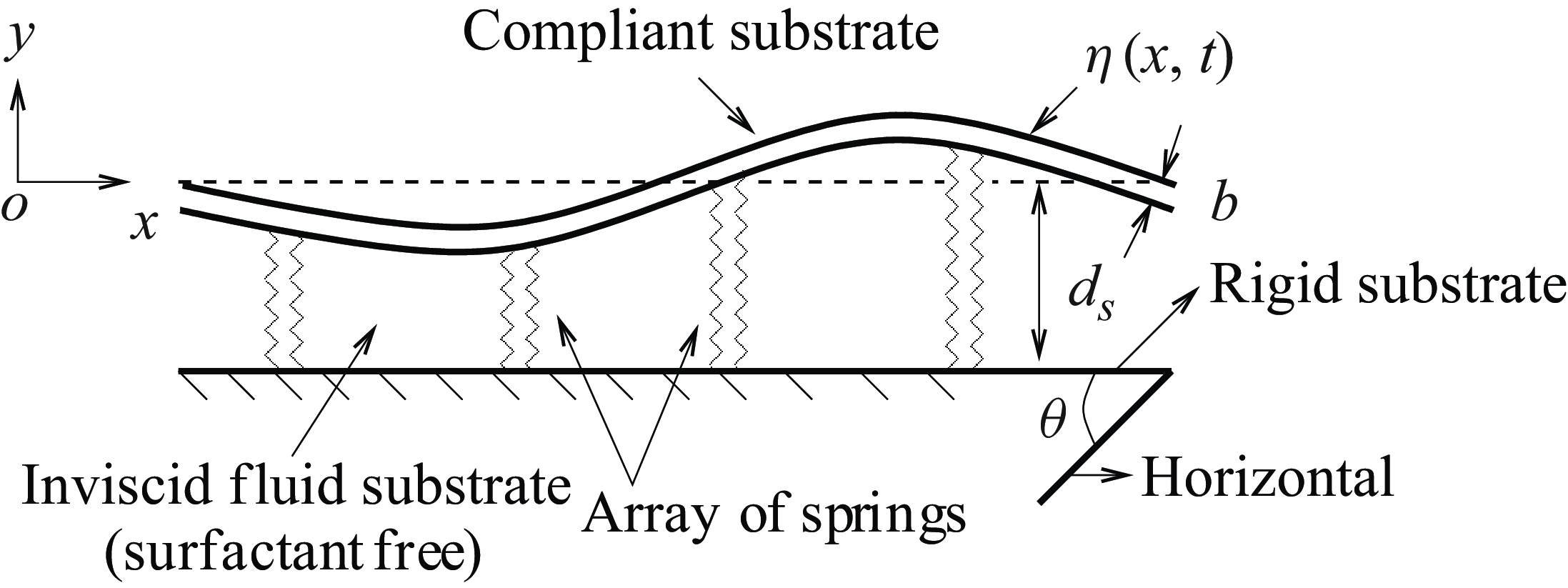
In an analogous fashion with the studies of Carpenter & Garrad (Reference Carpenter and Garrad1985) and Alexander et al. (Reference Alexander, Kirk and Papageorgiou2020), we use the same compliant-wall model as they proposed. This means that the compliant substrate is made up of an isotropic impermeable elastic plate or a tensorial membrane over a rigid substrate supported by an array of springs, as schematically illustrated in figure 2. In particular, we assemble the array of springs in such a way that the wavelength of the surface instability is sufficiently large in comparison with the distance between two neighbouring springs. We also fill the cavity between the elastic plate and the rigid substrate with a surfactant-free inviscid liquid with an equilibrium height of $d_s$ . This liquid is referred to as the substrate liquid. In addition, we assume that spring deformations have a negligible impact on the substrate liquid, but their effect on the elastic plate is included in the spring stiffness (Carpenter & Garrad Reference Carpenter and Garrad1985). Following the studies of Carpenter & Garrad (Reference Carpenter and Garrad1985) and Alexander et al. (Reference Alexander, Kirk and Papageorgiou2020), we employ a linear equation for the deflection, $\eta (x,t)$ , of the compliant substrate in the $y$ direction to show how its shape deforms from its equilibrium position:

(2.12) \begin{equation} \rho _w\,b\,\partial _{tt}\eta +D\partial _t\eta +B\partial _{xxxx}\eta -T\partial _{xx}\eta +K\eta =p_s-p+2\mu [\partial _yv-(\partial _yu+\partial _xv)\partial _x\eta ]. \end{equation}

Here $\rho _w$ denotes the density of the elastic material, $b$ denotes the thickness of the elastic plate, $D$ denotes the damping coefficient, $B$ denotes the flexural rigidity of the elastic plate, $T$ is the longitudinal tension and $K$ is the spring stiffness. Additionally, we assume that the elastic substrate is sufficiently thin so that the longitudinal tension $T$ remains uniform across its thickness (Matar et al. Reference Matar, Craster and Kumar2007). Here, $p_s$ is the pressure of the substrate liquid. The flexural rigidity $B$ and the damping coefficient $D$ can be measured from the material properties of the compliant substrate by using the following relationships (Carpenter & Garrad Reference Carpenter and Garrad1985; Alexander et al. Reference Alexander, Kirk and Papageorgiou2020):

(2.13) \begin{equation} B=\frac {E_Yb^3}{12(1-\nu ^2)}\ \textrm { and}\ D=2\zeta \sqrt {K \rho _w\, b}. \end{equation}

Here $E_Y$ denotes the Young’s modulus, $\nu$ denotes the Poisson ratio of the elastic material and $\zeta$ is the damping ratio. Clearly, the flexural rigidity $B$ and the damping coefficient $D$ are dependent parameters. As we have assumed an inviscid substrate liquid, (2.12) retains only the viscous effect of the mainstream liquid. Even though the disturbed mainstream liquid will cause the elastic plate to slightly deform from its equilibrium position, we assume that the pressure, $p_s$ , of the substrate liquid stays constant throughout at the equilibrium height, $d_s$ , from the rigid substrate (Alexander et al. Reference Alexander, Kirk and Papageorgiou2020). In fact, the variations in hydrostatic pressure are included in the spring stiffness $K$ (Carpenter & Garrad Reference Carpenter and Garrad1985). Moreover, the velocity components of the mainstream liquid must satisfy no-slip and kinematic conditions at the compliant substrate, $y=\eta (x,t)$ , (Matar et al. Reference Matar, Craster and Kumar2007; Peng et al. Reference Peng, Jiang, Zhuge and Zhang2016; Yang et al. Reference Yang, Jiang, Hu and Peng2018):

(2.14) \begin{equation} u=0,\ \ v=\partial _t\eta . \end{equation}

Finally, the no mass flux at the impermeable elastic plate, $y=\eta (x,t)$ , requires that

(2.15) \begin{equation} (\partial _x\eta \,\partial _xc_b - \partial _yc_b)=0. \end{equation}

Figure 2.

Sketch of an impermeable compliant substrate, where $b$ is the thickness of the compliant substrate that is supported by an array of springs. We assume that a surfactant-free inviscid liquid occupies the cavity between the elastic plate and the rigid substrate.

2.2. Dimensionless criterion

To make the above equations dimensionless, we have employed the following scaling:

(2.16) \begin{equation} \left . \begin{array}{ccccc} && \tilde {u}=\frac {u}{U_s},\ \ \tilde {v}=\frac {v}{U_s}, \ \ \tilde {p}=\frac {p d}{\mu U_s},\ \ \tilde {c}_b=\frac {dc_b}{\Gamma _{\infty }},\\ && \tilde {x}=\frac {x}{d},\ \ \tilde {y}=\frac {y}{d}, \ \ \tilde {h}=\frac {h}{d},\ \ \tilde {\eta }=\frac {\eta }{d}, \\ && \tilde {\Gamma }=\frac {\Gamma }{\Gamma _{\infty }},\ \ \tilde {t}=\frac {t U_s}{d}, \ \ \tilde {\sigma }=\frac {\sigma }{\sigma _0},\ \ \tilde {p}_a=\frac {p_a d}{\mu U_s}. \end{array} \right \} \end{equation}

Here $U_s=\rho g d^2\sin \theta /(2\mu )$ is the streamwise surface velocity for the steady uni-directional parallel flow of the mainstream liquid with a constant layer thickness, $d$ , when the compliant substrate has no deflection from its equilibrium position, $\eta =0$ . For our convenience, we have removed the tilde notation from the dimensionless equations in the subsequent mathematical expressions. Introducing the scaling (2.16) and performing dimensionless analysis, we can read the governing equations (2.1)--(2.4) in the following forms:

(2.17) \begin{align} &\qquad\qquad\qquad\qquad\qquad \partial _x u+\partial _y v=0, \end{align}

(2.18) \begin{align} &\quad Re(\partial _t u+u\partial _x u+v\partial _y u)=-\partial _x p+(\partial _{xx}u+\partial _{yy}u)+2, \end{align}

(2.19) \begin{align} & Re(\partial _t v+u\partial _x v+v\partial _y v)=-\partial _y p+(\partial _{xx}v+\partial _{yy}v)-2\cot \theta, \end{align}

(2.20) \begin{align} &\qquad\quad Pe_{b}(\partial _t c_b+u\partial _x c_b+v\partial _y c_b) =(\partial _{xx}c_b+\partial _{yy}c_b). \end{align}

Here $Re=\rho U_s d/\mu$ is the Reynolds number, which compares inertia to the viscous force, and $Pe_b=U_sd/D_b$ is the solutal Péclet number, which compares advective mass transport to diffusive mass transport in the bulk. After non-dimensionalization, at the liquid film surface, $y=h(x,t)$ , the associated boundary conditions (2.5)--(2.11) become

(2.21) \begin{align} &\qquad\quad \partial _t \Gamma +u\partial _x \Gamma + \frac {\Gamma }{1+(\partial _x h)^2}[\partial _xu+\partial _x h \partial _x v + \partial _x h(\partial _y u+\partial _x h \partial _y v)] \nonumber\\&\qquad\quad\quad=\frac {1}{Pe_s\sqrt {1+(\partial _x h)^2}}\partial _x\left [\frac {\partial _x\Gamma }{\sqrt {1+(\partial _x h)^2}}\right ]+k_s [\xi _s(1-\Gamma )c_b-\Gamma ], \end{align}

(2.22) \begin{align} &\qquad\quad\qquad\quad \frac {(\partial _x h\partial _x c_b - \partial _y c_b)}{Pe_b\sqrt {1+(\partial _x h)^2}} = k_s [\xi _s(1-\Gamma )c_b-\Gamma ], \end{align}

(2.23) \begin{align} &\qquad [4\partial _y v\partial _x h +(\partial _y u+\partial _x v)\{1-(\partial _x h)^2\}]+Ma_s \, \partial _x \Gamma \sqrt {1+(\partial _x h)^2}=0, \end{align}

(2.24) \begin{align} &\qquad\quad (p_a-p)+\frac {2}{[1+(\partial _x h)^2]}[\partial _y v\{1-(\partial _x h)^2\} - \partial _x h(\partial _y u +\partial _x v)]\nonumber\\&\qquad\qquad = [Ca^{-1}-Ma_{s}(\Gamma -\Gamma _E)]\frac {\partial _{xx} h}{[1+(\partial _x h)^2]^{3/2}}, \end{align}

(2.25) \begin{align} &\qquad\qquad\qquad\qquad\qquad \partial _t h+ u\partial _x h=v, \end{align}

where $Pe_s=U_sd/D_s$ is the surfactant Péclet number, which compares advective mass transport to diffusive mass transport at the film surface, $Ma_s=E\Gamma _{\infty }/(\mu U_s)$ is the surfactant Marangoni number, which compares the Marangoni stress to the viscous stress at the film surface, $Ca=\mu U_s/\sigma _0$ is the capillary number, which compares the viscous stress to the capillary stress generated by the surface tension of the mainstream liquid, and $\Gamma _E=\Gamma _0/\Gamma _{\infty }$ . As $\Gamma _{\infty }$ is the concentration of surface surfactant at the maximal packing, $\Gamma _E$ will belong to the range $0 \le \Gamma _E \le 1$ . Here, the parameter $k_s=({k_dd}/{U_s})=({{\rm d}/U_s}/{1/k_d})$ signifies the ratio of the convection time scale to the desorption time scale (Karapetsas & Bontozoglou Reference Karapetsas and Bontozoglou2014), and $\xi _{s}= ({k_a}/{k_dd})$ signifies the ratio of the adsorption and desorption rate constants. In fact, $\xi _s$ is the measure of surfactant solubility in the bulk. For instance, a small value of $\xi _s$ ( $ \ll 1$ ) indicates a situation of highly soluble surfactant, while a large value of $\xi _s$ ( $\gg 1$ ) indicates a situation of insoluble surfactant (Jensen & Grotberg (Reference Jensen and Grotberg1993)). Similarly, after non-dimensionalization, at the compliant substrate, $y=\eta (x,t)$ , the boundary conditions (2.12)--(2.15) become

(2.26) \begin{align} & C_{I}\partial _{tt}\eta +C_D\partial _t\eta +C_B\partial _{xxxx}\eta -C_T\partial _{xx}\eta +C_K\eta =(p_s-p)+2[\partial _yv-(\partial _yu+\partial _xv)\partial _x\eta ], \end{align}

(2.27) \begin{align} &\qquad\qquad\qquad\qquad\qquad\qquad u=0,\ \ v=\partial _t\eta, \end{align}

(2.28) \begin{align} &\qquad\qquad\qquad\quad\qquad\qquad (\partial _x\eta \partial _xc_b - \partial _yc_b)=0, \end{align}

where the material properties of the compliant substrate are represented by the following dimensionless parameters: $C_{I}=\rho _wb\,U_s/\mu$ , which specifies the ratio of compliant substrate inertia and the viscous stress; $C_{D}=Dd/\mu$ , which specifies the ratio of compliant substrate damping and the viscous stress; $C_B=B/(\mu d^2U_s)$ , which specifies the ratio of flexural rigidity and the viscous stress; $C_T=T/(\mu U_s)$ , which specifies the ratio of longitudinal tension and the viscous stress; $C_K=Kd^2/(\mu U_s)$ , which specifies the ratio of spring stiffness and the viscous stress.

2.3. Base flow solution

Here we want to find an analytical solution for a steady uni-directional soluble surfactant-laden parallel flow with a constant mainstream liquid layer thickness when the surfactant concentrations are uniform and the compliant substrate has no deflection from its equilibrium position. We also refer to the above flow as the base flow. Within the base flow approximations, we can set the partial derivatives with respect to $x$ and $t$ to zero. As a result, the governing equations and the associated boundary conditions (2.17)-- (2.28) are simplified, and their solution can be determined in the following form:

(2.29) \begin{equation} \left . \begin{array}{ccccc} && \bar {u}(y)=(2y-y^2),\ \ \bar {p}(y)=p_a+2\cot \theta (1-y),\ \ \bar {v}=0,\ \ \bar {h}=1,\\ && \bar {\Gamma }=\Gamma _E,\ \ \bar {c}_b=c_{E}=\frac {\Gamma _E}{\xi _s(1-\Gamma _E)},\ \ \bar {p}_s=p_a+2\cot \theta, \ \ \bar {\eta }=0. \end{array} \right \} \end{equation}

Here the bar notation serves as a representation of the base flow quantities. It should be useful to note that the dimensionless surfactant concentration $c_E$ in the bulk and the dimensionless surfactant concentration $\Gamma _E$ at the surface of the liquid film are both constants for the undisturbed parallel film flow with a uniform layer thickness, $\bar {h}=1$ , over an undeformed compliant substrate at a location $\bar {\eta }=0$ . Moreover, $\bar {c}_b$ approaches infinity when $\Gamma _E \to 1$ . Therefore, for the base surfactant concentration, $\bar {c}_b=c_E$ , in the bulk to have a bounded value, $\xi _s$ must approach infinity ( $\xi _s \to \infty$ ) so that the product term, $\xi _s(1-\Gamma _E)$ , will be finite when $\Gamma _E \to 1$ . However, if $\xi _s(1-\Gamma _E) \to \infty$ , the base surfactant concentration, $\bar {c}_b$ , in the bulk vanishes and causes a situation of an insoluble surfactant-laden film flow (D’Alessio et al. Reference D’Alessio, Pascal, Ellaban and Ruyer-Quil2020). We will later use this limiting condition to verify the results of an insoluble surfactant-laden film flowing over a compliant wall.

3.1. Long-wave series assumption

To decipher the primary instability in the long-wave regime ( $k \sim (1/\lambda ) \to 0$ , where $\lambda$ is the wavelength of the infinitesimal disturbance), the following long-wave series expansions are proposed (Yih Reference Yih1963; Smith Reference Smith1990; Samanta Reference Samanta2019):

(3.25) \begin{align} \left . \begin{array}{clc} \hat {u}(y)& \!\!\! = \!\!\! & \hat {u}_0+k\hat {u}_1+k^2\hat {u}_2+\cdots, \\ \hat {v}(y)& \!\!\! = \!\!\! & k\hat {v}_1+k^2\hat {v}_2+k^3\hat {v}_3+\cdots, \\ \hat {c}_b(y)& \!\!\! = \!\!\! & \hat {c}_{b0}+k\hat {c}_{b1}+k^2\hat {c}_{b2}+\cdots, \\ \hat {p}(y)& \!\!\! = \!\!\! & \hat {p}_0+k\hat {p}_1+k^2\hat {p}_2+\cdots, \\ \hat {h}& \!\!\! = \!\!\! & \hat {h}_0+k\hat {h}_1+k^2\hat {h}_2+\cdots, \\ \hat {\eta }& \!\!\! = \!\!\! & \hat {\eta }_0+k\hat {\eta }_1+k^2\hat {\eta }_2+\cdots, \\ \hat {\Gamma }& \!\!\! = \!\!\! & \hat {\Gamma }_0+k\hat {\Gamma }_1+k^2\hat {\Gamma }_2+\cdots, \\ c& \!\!\! = \!\!\! & c_0+kc_1+k^2c_2+\cdots . \end{array} \right \}\nonumber\\[-18pt] \end{align}

Since the long-wave series expansions (3.25) are written in the limit $k \to 0$ , they are appropriate only in the small neighbourhood of $k=0$ . As soon as $k$ increases, there is a convergence issue. This makes the long-wave series impossible to determine the short-wave unstable mode, but we can capture the long-wave unstable mode by using these series expansions (3.25). To detect the unstable modes that emerge in the finite-wavelength regime, we shall employ the numerical technique discussed in the next section.

3.2. Zeroth-order [ $\mathcal{O}(k^0)$ ] long-wave analysis

After plugging the series expansions (3.25) into (3.14)--(3.24), we collect the zeroth-order $[\mathcal{O}(k^0)]$ long-wave equations:

(3.26) \begin{align} &\qquad\qquad D^2\hat {u}_0=0,\quad D\hat {p}_0=0,\quad D^2\hat {c}_{b0}=0,\quad 0 \le y \le 1, \end{align}

(3.27) \begin{align} &\quad D\hat {u}_0+\hat {h}_0D^2\bar {u}=0,\quad \hat {p}_0-2 \cot \theta \,\hat {h}_0=0,\quad D\hat {c}_{b0}=0,\quad \textrm { at}\ y=1, \end{align}

(3.28) \begin{align} & C_K\hat {\eta }_0+\hat {p}_0-2\cot \theta \,\hat {\eta }_0=0,\quad \hat {u}_0+D\bar {u}\,\hat {\eta }_0 =0,\quad D\hat {c}_{b0}=0,\quad\textrm { at}\ y=0. \end{align}

Here, we have assumed that the capillary number $Ca$ is of order one, i.e. $Ca \sim \mathcal{O}(1)$ . As a result, the capillary number does not appear in the zeroth-order normal stress boundary condition. After solving, we express the solution of the zeroth-order long-wave equations (3.26)--(3.28) in the form

(3.29) \begin{align} & \hat {u}_0(y)=2(\hat {h}_0y-\hat {\eta }_0),\ \ \hat {p}_0(y)=2\cot \theta \hat {h}_0,\ \ \hat {c}_{b0}(y)=\frac {(1+\xi _sc_E)\hat {\Gamma }_0}{\xi _s(1-\Gamma _E)}, \end{align}

(3.30) \begin{align} &\qquad \hat {\eta }_0=-\left [\frac {2\cot \theta }{(C_K - 2\cot \theta )}\right ]\hat {h}_0=-\left [\frac {2\cot \theta /C_K}{(1 - 2\cot \theta /C_K)}\right ]\hat {h}_0, \end{align}

provided $\xi _s(1-\Gamma _E) \neq 0$ and $(C_k - 2\cot \theta ) \neq 0$ . Denote by $C_k^*=2\cot \theta$ , the critical value of the non-dimensional spring stiffness coefficient $C_K$ . Therefore, if $\hat {h}_0 \gt 0$ and $\theta \neq 0$ , $\hat {\eta }_0 \rightarrow 0$ in the limit $\theta \to \pi /2$ or $C_K \to \infty$ , indicating a rigid impermeable wall. Hence, when $0 \lt \theta \lt \pi /2$ and $\hat {h}_0 \gt 0$ , the zeroth-order amplitude, $\hat {\eta }_0$ , of the compliant substrate deformation will be out-of-phase with or in-phase with the zeroth-order amplitude, $\hat {h}_0$ , of the liquid film surface deformation depending on whether $C_K\gt C_K^{*}$ or $C_K \lt C_K^*$ . It is important to note that the zeroth-order amplitude of the streamwise perturbation velocity, $\hat {u}_0(y)$ , is a linear function of the cross-stream coordinate, $y$ , and explicitly depends on the spring stiffness coefficient $C_K$ and the inclination angle $\theta$ . Clearly, the expression of $\hat {u}_0(y)$ is different from that of film flowing over a non-compliant impermeable substrate (Smith Reference Smith1990). In fact, the presence of a compliant substrate significantly affects the zeroth-order amplitude of the streamwise perturbation velocity. Specifically, if $\hat {h}_0\gt 0$ , it will accelerate or decelerate depending on whether the zeroth-order amplitude of the compliant substrate deformation is out-of-phase with or in-phase with the zeroth-order amplitude of the liquid film surface deformation. Therefore, it certainly depends on the non-dimensional spring stiffness coefficient $C_K$ . Furthermore, we see that the zeroth-order amplitude of the perturbation surfactant concentration, $\hat {c}_{b0}$ , in the bulk approaches zero in the limit $\xi _s(1-\Gamma _E) \to \infty$ . This creates a situation of an insoluble surfactant-laden film flowing over a compliant substrate (Samanta Reference Samanta2021a ).

3.3. First-order [ $\mathcal{O}(k^1)$ ] long-wave analysis

The first-order long-wave equations $[\mathcal{O}(k^1)]$ are

(3.31) \begin{align} &\qquad\qquad\qquad\qquad i\hat {u}_0+D\hat {v}_1=0,\quad 0 \le y \le 1,\\[-8pt]\nonumber \end{align}

(3.32) \begin{align} &\qquad Re[i(\bar {u}-c_0)\hat {u}_0+D\bar {u}\,\hat {v}_1]+i\hat {p}_0-D^2\hat {u}_1=0,\quad 0 \le y \le 1,\\[-8pt]\nonumber \end{align}

(3.33) \begin{align} &\qquad\qquad\qquad\qquad D\hat{p}_1-D^2\hat{v}_1=0, 0 \le y \le 1,\\[-8pt]\nonumber \end{align}

(3.34) \begin{align} &\qquad\qquad\qquad iPe_b(\bar {u}-c_0)\hat {c}_{b0}-D^2\hat {c}_{b1}=0,\quad 0 \le y \le 1,\\[-8pt]\nonumber \end{align}

(3.35) \begin{align} &\qquad\qquad D\hat {c}_{b1}+iPe_b[(\bar {u}-c_0)\hat {\Gamma }_{0}+\Gamma _E\hat {u}_0]=0\quad \textrm { at}\ y=1,\\[-8pt]\nonumber \end{align}

(3.36) \begin{align} &\qquad\qquad\qquad D\hat {u}_1+\hat {h}_1D^2\bar {u}+iMa_s\hat {\Gamma }_0=0\quad \textrm { at}\ y=1,\\[-8pt]\nonumber \end{align}

(3.37) \begin{align} &\qquad\qquad\qquad -\hat {p}_1+2 \cot \theta \hat {h}_1+2D\hat {v}_1=0\quad \textrm { at}\ y=1,\\[-8pt]\nonumber \end{align}

(3.38) \begin{align} &\qquad\qquad\qquad\qquad\quad i(\bar {u}-c_0)\hat {h}_0-\hat {v}_1=0\quad\textrm { at}\ y=1,\\[-8pt]\nonumber \end{align}

(3.39) \begin{align} & -iC_D\,c_0\hat {\eta }_0+C_K\hat {\eta }_1+\hat {p}_1-2\cot \theta \hat {\eta }_1-2[D\hat {v}_1-iD\bar {u}\,\hat {\eta }_0]=0\quad \textrm { at}\ y=0,\\[-8pt]\nonumber \end{align}

(3.40) \begin{align} &\qquad\qquad\qquad\qquad\qquad \hat {u}_1+D\bar {u}\hat {\eta }_1 =0\quad\textrm {at}\ y=0,\\[-8pt]\nonumber \end{align}

(3.41) \begin{align} &\qquad\qquad\qquad\qquad\qquad \hat {v}_1+ic_0\hat {\eta }_0=0\quad\textrm {at}\ y=0,\\[-8pt]\nonumber \end{align}

(3.42) \begin{align} &\qquad\qquad\qquad\qquad\qquad\quad D\hat {c}_{b1}=0\quad \textrm {at}\ y=0. \end{align}

The solution of the first-order long-wave equations (3.31)--(3.42) can be expressed as

(3.43) \begin{align} \hat {u}_1(y) & =\hat {h}_0\left [iRe\left \{\frac {1}{6}y^4-\frac {1}{3}c_0y^3-\frac {2}{3}y+c_0y\right \}+i\cot \theta ( y^2-2y)\right ]\nonumber\\& \quad + 2\hat {h}_{1}y-iMa_s\,\hat {\Gamma }_{0}\,y-iRe\left \{\frac {1}{6}y^4-\frac {1}{3}c_0y^3-\frac {2}{3}y+c_0y\right \}\hat {\eta }_0-2\hat {\eta }_1, \end{align}

(3.44) \begin{align} &\qquad\qquad\qquad\qquad \hat {v}_1(y)=-i\hat {h}_0y^2+2i\hat {\eta }_0y-i\hat {\eta }_0c_0, \end{align}

(3.45) \begin{align} &\qquad\qquad\qquad \hat {p}_1(y)=-2i\hat {h}_0y-2i\hat {h}_0+2\cot \theta \hat {h}_1+4i\hat {\eta }_0, \end{align}

(3.46) \begin{align} &\qquad\qquad\qquad \hat {\eta }_1=\frac {-2\cot \theta \hat {h}_1+i(2\hat {h}_0-4\hat {\eta }_0+C_Dc_0\hat {\eta }_0)}{(C_K-2\cot \theta )}, \end{align}

(3.47) \begin{align} &\qquad\qquad\qquad\qquad \hat {\Gamma }_0=\frac {6\Gamma _E\xi _s(1-\Gamma _E)^2(\hat {h}_0-\hat {\eta }_0)}{4+3\xi _s(1-\Gamma _E)^2}, \end{align}

(3.48) \begin{align} &\qquad\qquad\qquad\qquad\qquad\qquad\qquad c_0=2. \end{align}

As discussed by Wei (Reference Wei2005); Bhat & Samanta (Reference Bhat and Samanta2018) and Samanta (Reference Samanta2021a ), two dominant temporal modes, the so-called surface mode and surfactant mode, can be obtained analytically using the long-wave analysis for a shear-imposed film flow when the free surface is contaminated by an insoluble surfactant. However, it is important to note that the surfactant mode appears and becomes unstable when the zeroth-order amplitude, $\hat {h}_0$ , of the film surface deformation vanishes ( $\hat {h}_0=0$ ) and the constant surface shear stress is present. Therefore, if we impose an infinitesimal perturbation on the surface of a steady uni-directional parallel film flow, the surface will always deflect from its flat position. Hence, $\hat {h}_0$ , cannot be zero physically as long as we concern ourselves with the perturbation of the liquid film surface. Furthermore, the film surface is free of external shear stress. These factors make the existence of an unstable surfactant mode impossible in the current study, and therefore, we will only deal with the surface mode in the long-wave analysis. The analytical calculation reveals that the presence of a soluble surfactant or a compliant substrate has no effect on the zeroth-order phase speed, which is $c_0=2$ . Furthermore, it is two times ( $c_0=2\bar {u}|_{y=1}$ ) the liquid film surface velocity of a steady basic parallel film flow. Additionally, we observe that the zeroth-order amplitude $\hat {\Gamma }_0$ of the surface surfactant is explicitly dependent on the zeroth-order amplitude, $\hat {\eta }_0$ , of the compliant substrate deformation. However, if we implement the limit of the situation of an insoluble surfactant, $\xi _s(1-\Gamma _E) \to \infty$ , the current result matches very well with that of Samanta (Reference Samanta2021a ) when the imposed shear stress is absent at the film surface, and it can be read as

(3.49) \begin{equation} \frac{\hat {\Gamma }_0}{\Gamma _E}=2(\hat {h}_0-\hat {\eta }_0)=\left [\frac {2\hat {h}_0C_K}{(C_K-2\cot \theta )}\right ]=\left [\frac {2\hat {h}_0}{(1-2\cot \theta /C_K)}\right ]. \end{equation}

Obviously, $\hat {\Gamma }_0/\Gamma _E \to 2\hat {h}_0$ in the limit $C_K \to \infty$ or $\theta \to \pi /2$ . This result indicates that the zeroth-order amplitude of the surface surfactant is twice the zeroth-order amplitude of the liquid film surface deformation due to an infinitesimal perturbation if the surface surfactant concentration is scaled by the base surface surfactant concentration instead of the surface surfactant concentration at maximal packing and when the compliant wall acts like a rigid impermeable wall ( $C_K \to \infty$ ). This result is in agreement with that of Wei (Reference Wei2005) in the absence of imposed shear stress at the film surface. Moreover, the zeroth-order perturbation surfactant concentration, $\hat {\Gamma }_0$ , will be in-phase with or out-of-phase with the zeroth-order liquid surface deformation, $\hat {h}_0$ , if $C_K\gt C_K^*$ or $C_K\lt C_K^*$ . This physical phenomenon is completely opposite to that of the zeroth-order compliant substrate deformation.

3.4. Second-order [ $\mathcal{O}(k^2)$ ] long-wave analysis

The second-order $[\mathcal{O}(k^2)]$ long-wave equations are

(3.50) \begin{align} &\qquad\qquad\qquad\qquad\qquad i\hat {u}_1+D\hat {v}_2=0,\quad 0 \le y \le 1, \end{align}

(3.51) \begin{align} & Re[i(\bar {u}-c_0)\hat {u}_1-ic_1\hat {u}_0+D\bar {u}\,\hat {v}_2]+i\hat {p}_1-(D^2\hat {u}_2-\hat {u}_0)=0,\quad 0 \le y \le 1, \end{align}

(3.52) \begin{align} &\qquad\qquad\qquad Rei(\bar {u}-c_0)\hat {v}_1+D\hat {p}_2-D^2\hat {v}_2=0,\quad 0 \le y \le 1, \end{align}

(3.53) \begin{align} &\qquad\qquad iPe_b[(\bar {u}-c_0)\hat {c}_{b1}-c_1\hat {c}_{bo}]-(D^2\hat {c}_{b2}-\hat {c}_{b0})=0,\quad 0 \le y \le 1, \end{align}

(3.54) \begin{align} & D\hat {c}_{b2}+iPe_b[(\bar {u}-c_0)\hat {\Gamma }_{1}-c_1\hat {\Gamma }_0+\Gamma _E\,\hat {u}_1]+\left(\frac{Pe_b}{Pe_s}\right)\hat {\Gamma }_0=0\quad \textrm {at}\ y=1, \end{align}

(3.55) \begin{align} &\qquad\qquad\qquad D\hat {u}_2+i\hat {v}_1+\hat {h}_2D^2\bar {u}+iMa_s\hat {\Gamma }_1=0\quad \textrm {at}\ y=1, \end{align}

(3.56) \begin{align} &\qquad\qquad\quad -\hat {p}_2+2 \cot \theta \hat {h}_2+2D\hat {v}_2+\left(\frac{1}{Ca}\right)\hat {h}_0=0\quad \textrm {at}\ y=1, \end{align}

(3.57) \begin{align} &\qquad\qquad\qquad\quad i(\bar {u}-c_0)\hat {h}_1-ic_1\hat {h}_0-\hat {v}_2=0\quad \textrm {at}\ y=1, \end{align}

(3.58) \begin{align} &\quad -C_Ic_0^2\hat {\eta }_0-iC_D(c_0\hat {\eta }_1+c_1\hat {\eta }_0)+C_T\hat {\eta }_0+C_K\hat {\eta }_2+\hat {p}_2-2\cot \theta \hat {\eta }_2\nonumber\\&\qquad\qquad\qquad\qquad -2[D\hat {v}_2-iD\bar {u}\hat {\eta }_1]=0\quad \textrm {at} \ y=0, \end{align}

(3.59) \begin{align} &\qquad\qquad\qquad\qquad\qquad \hat {u}_2+D\bar {u}\hat {\eta }_2 =0\quad \textrm {at}\ y=0, \end{align}

(3.60) \begin{align} &\qquad\qquad\qquad\qquad \hat {v}_2+i(c_0\hat {\eta }_1+c_1\hat {\eta }_0)=0\quad \textrm {at} \ y=0, \end{align}

(3.61) \begin{align} &\qquad\qquad\qquad\qquad\qquad\quad D\hat {c}_{b2}=0\quad \textrm {at} \ y=0. \end{align}

After solving the above second-order long-wave equations (3.50)--(3.61), we finally evaluate the expression of $c_1$ from the kinematic boundary condition (3.57):

(3.62) \begin{equation} c_1=i\left [\frac {8}{15}Re-\frac {2}{3}\cot \theta +\frac {4}{3} \frac {\cot ^2\theta }{C_K} -\frac {3Ma_s\Gamma _E\xi _s(1-\Gamma _E)^2}{4+3\xi _s(1-\Gamma _E)^2}\right ]. \end{equation}

As the temporal growth rate $kc_i \approx k^2|c_1|$ in the limit $k \to 0$ , in expression (3.62), the first term provides a destabilizing contribution of inertia, the second term provides a stabilizing contribution of depthwise gravity, the third term provides a destabilizing contribution of compliant substrate and the fourth term provides a stabilizing contribution of surfactant to the temporal growth rate corresponding to the surface mode. Using the neutral stability condition ( $c_i \approx k|c_1|=0$ as $k \to 0$ ), we calculate the critical Reynolds number for the surface mode:

(3.63) \begin{equation} Re_c=\underbrace {\frac {5}{4}\cot \theta }_{\textrm { Effect of depthwise gravity}} - \underbrace {\frac {5}{2}\frac {\cot ^2\theta }{C_K}}_{\textrm { Effect of compliant wall}} + \underbrace {\frac {45}{8}\left [\frac {Ma_s\Gamma _E\xi _s(1-\Gamma _E)^2}{4+3\xi _s(1-\Gamma _E)^2}\right ]}_{\textrm { Effect of surfactant}}. \end{equation}

Clearly, we see that the critical Reynolds number $Re_{c}$ , or the onset of surface instability, has a deviation from its known value, $Re_c=({5}/{4})\cot \theta$ , for a surfactant-free film flow over a non-compliant wall (Benjamin Reference Benjamin1957; Yih Reference Yih1963) due to the presence of a soluble surfactant and a compliant substrate at the bottom. In particular, $Re_{c}$ increases in the presence of a soluble surfactant but decreases in the presence of a compliant substrate. Hence, the soluble surfactant has a stabilizing influence, while the compliant substrate has a destabilizing influence on surface instability. Since the soluble surfactant and the compliant wall have opposing impacts on surface instability, they will be nullified once the second and third terms in (3.63) are equal, which yields the expression

(3.64) \begin{equation} \frac {Ma_s\Gamma _E\xi _s(1-\Gamma _E)^2}{4+3\xi _s(1-\Gamma _E)^2} = \frac {4}{9}\frac {\cot ^2\theta }{C_K}. \end{equation}

Therefore, with the aid of the linear stability analysis, we can predict parameter combinations related to the soluble surfactant and compliant wall, which will ensure the same critical Reynolds number for the emergence of surface instability for the gravity-driven surfactant-laden film flowing over a compliant wall and the gravity-driven surfactant-free film flowing over a non-compliant wall. Furthermore, we note that $Re_c$ for surface instability coincides with the result of Alexander et al. (Reference Alexander, Kirk and Papageorgiou2020) in the absence of surfactant, i.e. when we omit the third term in (3.63). The expression is given below:

(3.65) \begin{equation} Re_c=\frac {5}{4}\cot \theta -\frac {5}{2}\frac {\cot ^2\theta }{C_K}. \end{equation}

If the effect of a compliant substrate is ignored, i.e. when we neglect the second term in (3.63), the result of Karapetsas & Bontozoglou (Reference Karapetsas and Bontozoglou2014) is recovered. The expression is presented below:

(3.66) \begin{equation} Re_c=\frac {5}{4}\cot \theta +\frac {45}{8}\left [\frac {Ma_s\Gamma _E\xi _s(1-\Gamma _E)^2}{4+3\xi _s(1-\Gamma _E)^2}\right ]. \end{equation}

Next, if we take the limit of insoluble surfactant $[\xi _s(1-\Gamma _E) \to \infty ]$ in (3.63), the result of Samanta (Reference Samanta2021a ) is captured, which can be expressed as

(3.67) \begin{equation} Re_c=\frac {5}{4}\cot \theta -\frac {5}{2}\frac {\cot ^2\theta }{C_K}+\frac {15}{8}Ma_s\Gamma _E. \end{equation}

These events are further demonstrated in figure 3(a) through the variation of the critical Reynolds number for surface instability as the parameter $\xi _s$ alters. We can see that $Re_c$ decreases with decreasing $\xi _s$ and approaches the critical Reynolds number for the surfactant-free film flowing over a compliant wall (Alexander et al. Reference Alexander, Kirk and Papageorgiou2020) when $\xi _s \to 0$ . In contrast, $Re_c$ approaches the critical Reynolds number for an insoluble surfactant-laden film flowing over a compliant wall (Samanta Reference Samanta2021a ) when the parameter $\xi _s$ becomes very large. In fact, $Re_c$ increases with increasing $\xi _s$ in $0 \lt \Gamma _E \lt 1$ , indicating a stabilizing effect for higher values of the ratio of adsorption and desorption rate constants. So, if the film surface adsorbs more surfactant from the bulk, the surface tension will reduce, and the linearly unstable flow will gradually become stable. Additionally, we note that there is a maximum of $Re_c$ in each curve in the range $0 \lt \Gamma _E \lt 1$ , and this maximum shifts towards $\Gamma _E \approx 1$ as $\xi _s \to \infty$ . To figure out the reason why $Re_c$ for the onset of surface instability reaches its maximum at a specific value of $\Gamma _E$ for a given value of $\xi _s$ , we write the third term of (3.63) in a functional form:

(3.68) \begin{equation} Re_{\Gamma }(Ma_s,\Gamma _E,\xi _s)=\frac {45}{8}\left [\frac {Ma_s\Gamma _E\xi _s(1-\Gamma _E)^2}{4+3\xi _s(1-\Gamma _E)^2}\right ]. \end{equation}

Then, $({\partial Re_{\Gamma }}/{\partial \Gamma _E})=0$ leads to the following quartic polynomial equation of $\Gamma _E$ whose coefficients are functions of $\xi _s$ :

(3.69) \begin{equation} (\Gamma _E-1)[3\xi _s\Gamma _E^3-9\xi _s\Gamma _E^2+(9\xi _s+12)\Gamma _E-(3\xi _s+4)]=0. \end{equation}

Therefore, roots of (3.69) provide the local maximums or local minimums for the function $Re_{\Gamma }(Ma_s,\Gamma _E,\xi _s)$ . Using the condition for the second derivative $ ({\partial ^2 Re_{\Gamma }}/{\partial \Gamma _E^2})\lt 0$ , we determine the expression of $\Gamma _E$ for which the function $Re_{\Gamma }(Ma_s,\Gamma _E,\xi _s)$ has a local maximum, and the expression is given below:

(3.70) \begin{equation} \Gamma _E=1-\frac {2(2/3)^{1/3}}{a_{\xi }}+\frac {(2/3)^{2/3}a_{\xi }}{\xi _s},\ \textrm { where}\ a_{\xi }=[-3\xi _s^2+\sqrt {3}\sqrt {4\xi _s^3+3\xi _s^4}]^{1/3}. \end{equation}

Figure 3.

(a) Variation of the critical Reynolds number for the onset of surface instability as the parameter $\xi _s$ changes when $C_K=5$ . Solid, dashed, dotted and dash-dotted lines stand for $\xi _s=10^3$ , $\xi _s=10^2$ , $\xi _s=10^1$ and $\xi _s=10^0$ , respectively. The circle and cross symbols are the results of Samanta (Reference Samanta2021a ) and Alexander et al. (Reference Alexander, Kirk and Papageorgiou2020), respectively. (b) Variation of the critical Reynolds number for the onset of surface instability as the parameter $C_K$ changes when $\xi _s=10^3$ . Solid, dashed and dotted lines stand for $C_K=5$ , $C_K=10$ and $C_K=100$ , respectively. The circle symbols are the results of Wei (Reference Wei2005). The triangle symbol represents the maximum value of the critical Reynolds number on each curve. Thin dashed lines in figures 3(a) and 3(b) represent for the maximum value of the critical Reynolds number for varying $\xi _s$ and $C_K$ , respectively. The other parameters are $Ma_s=1$ and $\theta =45^{\circ }$ .

The maximum value of the critical Reynolds number for surface instability at this $\Gamma _E$ is further plotted in figure 3(a) by a thin dashed line, which, indeed, passes through the maximum of the critical Reynolds number for surface instability in the range $0 \lt \Gamma _E \lt 1$ when $\xi _s$ varies. The above physical phenomenon was also observed in experiment and theory by Georgantaki, Vlachogiannis & Bontozoglou (Reference Georgantaki, Vlachogiannis and Bontozoglou2016) and Katsiavria & Bontozoglou (Reference Katsiavria and Bontozoglou2020) for a soluble surfactant-laden film flowing down a rigid impermeable wall. In the spirit of their discussions, a perturbation shear stress is developed at the film surface whenever the surface is disturbed by an infinitesimal perturbation (Smith Reference Smith1990). This fact also causes perturbation in surface surfactant concentration and generates surface elasticity due to changes in surface tension along the surface because surfactant concentration is higher at the crest and lower at the trough, as it is in-phase with the deformed film surface. The generated surface elasticity induces the Marangoni stress, which counteracts surface deformation and stabilizes surface instability. As the current study deals with the soluble surfactant-laden film flow, the situation differs non-trivially from the study of the insoluble surfactant-laden film flow. In particular, because of the local equilibrium, the velocity perturbations trigger both the perturbation in surface surfactant concentration and the perturbation in bulk surfactant concentration in the vicinity of the film surface. As a consequence, the concentration gradient is developed across the film surface due to the mass exchange between surface and bulk surfactant concentrations, which counteracts the interfacial gradient of $\Gamma (x,t)$ and mitigates the Marangoni stress-induced stabilizing flow (Karapetsas & Bontozoglou Reference Karapetsas and Bontozoglou2014; Georgantaki et al. Reference Georgantaki, Vlachogiannis and Bontozoglou2016). Physically, the increase in surfactant concentration at the film surface can be attributed to either the adsorption of surfactant from the bulk for increasing $\xi _s$ or the increase of base surface surfactant concentration for increasing $\Gamma _E$ . As $\Gamma _E$ rises, a surfactant concentration gradient forms along the film surface, where concentration is higher at the crest and lower at the trough as the perturbation film surface and perturbation surfactant concentration are in the same phase. Consequently, surface tension is low at the crest and high at the trough. This fact also makes the surface elasticity stronger and creates a local flow at the film surface from crest to trough direction due to the Marangoni stress, which suppresses surface instability. If the base surface surfactant concentration is further increased, the surface elasticity is intensified. But as the bulk surfactant concentration rises, there is more mass exchange between bulk and surface surfactant concentrations close to the surface. This cancels out the effect of elasticity and makes the film surface look like the surface without surfactant (Georgantaki et al. Reference Georgantaki, Vlachogiannis and Bontozoglou2016). That is why the value of $Re_c$ at $\Gamma _E = 1$ coincides with that at $\Gamma _E=0$ . From the above findings, one can also conclude that the film flow with a soluble surfactant is linearly more unstable than the film flow with an insoluble surfactant. In continuation of the above case $[\xi _s(1-\Gamma _E) \to \infty ]$ , if we take the limit $C_K \to \infty$ , which means that the spring stiffness coefficient is very high, the contribution corresponding to the compliant substrate to the critical Reynolds number for the onset of surface instability vanishes. This is because the compliant substrate behaves as a rigid substrate (Alexander et al. Reference Alexander, Kirk and Papageorgiou2020). As a result, the critical Reynolds number simplifies to the case of an insoluble surfactant-laden film flowing down a non-compliant wall (Wei Reference Wei2005), and it can be read as

(3.71) \begin{equation} Re_c=\frac {5}{4}\cot \theta + \frac {15}{8}Ma_s\Gamma _E. \end{equation}

We have depicted this result through the variation of the critical Reynolds number in figure 3(b) as the parameter $C_K$ alters. Clearly, $Re_c$ tends to the critical Reynolds number for an insoluble surfactant-laden film flowing down a non-compliant wall (Wei Reference Wei2005) for a large value of $C_K$ . Moreover, $Re_c$ decreases with decreasing $C_K$ , indicating a destabilizing effect for lower values of the spring stiffness coefficient. In addition, we see a maximum of $Re_c$ on each curve at a fixed $\Gamma _E$ , irrespective of the changes in value of $C_K$ . This is also demonstrated by a thin dashed line in figure 3(b). Hence, $C_K$ has no influence on $\Gamma _E$ . For our convenience, we further arrange (3.63) of the critical Reynolds number, $Re_c$ , in the following form:

(3.72) \begin{equation} Re_c=\frac {5}{4} \cot \theta \left [1 -\frac {2 \cot \theta }{C_K}\right ]+\frac {45}{8}\left [\frac {Ma_s\Gamma _E\xi _s(1-\Gamma _E)^2}{4+3\xi _s(1-\Gamma _E)^2}\right ]. \end{equation}

Equation (3.72) shows that the destabilizing influence of the compliant substrate on surface instability becomes weaker with the increase in value of the spring stiffness coefficient $C_K$ from its value $C_K^*=2\cot \theta$ ( $C_K\gt C_K^*$ ). By contrast, if $C_K\lt C_K^*$ , the base flow system eventually turns into a linearly unstable flow to an infinitesimal disturbance in the absence of a soluble surfactant. This is because $Re_c$ becomes zero at $C_K = C_K^*$ , and it becomes negative when $C_K\lt C_K^*$ . However, if the soluble surfactant is present, $Re_c$ can be positive once the following criterion is satisfied:

(3.73) \begin{equation} \frac {Ma_s\Gamma _E\xi _s(1-\Gamma _E)^2}{4+3\xi _s(1-\Gamma _E)^2} \gt \frac {2\cot \theta }{9}\left [\frac {2\cot \theta }{C_K}-1\right ]. \end{equation}

Therefore, if condition (3.73) holds, there exists a range of the Reynolds number where the base flow will be linearly stable to infinitesimal disturbances. Finally, if we consider the case of a vertically compliant wall [ $\theta =\pi /2$ ], (3.63) reduces to the following form:

(3.74) \begin{equation} Re_c=\frac {45}{8}\left [\frac {Ma_s\Gamma _E\xi _s(1-\Gamma _E)^2}{4+3\xi _s(1-\Gamma _E)^2}\right ]. \end{equation}

Apparently, there is no contribution from the compliant wall to the expression of the critical Reynolds number for the onset of surface instability. As a result, the base flow can be stable to infinitesimal disturbances in a certain range of the Reynolds number due to the presence of a soluble surfactant, even though the flow occurs on a vertically compliant wall. This is the exact opposite of what happens when a clean liquid film flows over a vertically non-compliant wall. In that case, the film flow is susceptible to instability under infinitesimal disturbances for a non-zero $Re$ because $Re_c=0$ . Figure 4 displays the variation of the critical Reynolds number for the onset of surface instability in the ( $C_K$ , $Re_c$ ) plane when the parameter $\xi _s$ alters. If $\xi _s$ is very small, the critical Reynolds number converges to the result of Alexander et al. (Reference Alexander, Kirk and Papageorgiou2020), which is specified by a curve with star symbols. In particular, the critical Reynolds number approaches zero at $C_K \approx 2$ because the surfactant contribution to the critical Reynolds number becomes negligible at $\Gamma _E=0.1$ , $Ma_s=1$ , $\theta =45^{\circ }$ and $\xi _s=10^{-1}$ . As soon as $\xi _s$ increases, the critical Reynolds number no longer becomes zero at $C_K=2$ but becomes positive due to the contribution of surfactant, which creates a range of $Re$ for a linearly stable flow. Finally, when $\xi _s$ becomes very large, the critical Reynolds number converges to the result of Samanta (Reference Samanta2021a ), which is specified by a curve with circle symbols.

Figure 4.

Variation of the critical Reynolds number for the onset of surface instability as the parameter $\xi _s$ changes when $Ma_s=1$ , $\theta =45^{\circ }$ and $\Gamma _E=0.1$ . Solid, dashed and dotted lines stand for $\xi _s=10^3$ , $\xi _s=10^0$ and $\xi _s=10^{-1}$ , respectively. The circle and star symbols are the results of Samanta (Reference Samanta2021a ) and Alexander et al. (Reference Alexander, Kirk and Papageorgiou2020), respectively. The solid red points represent the range of $Re$ for a linearly stable flow.

3.5. Physical mechanism of surface instability

Now we shall discuss the physical mechanism of surface instability for the present flow configuration based on the speed of a linear hyperbolic wave. As a result, we integrate the perturbation continuity equation (3.2) with respect to $y$ over the domain $[0, 1]$ and use the kinematic boundary conditions (3.10) and (3.12) at the film surface and the compliant wall, respectively. This leads to the following mass conservation equation for the perturbation flow:

(3.75) \begin{equation} \partial _th^{\prime}+\bar {u}|_{y=1}\partial _xh^{\prime}+\partial _xq^{\prime}-\partial _t\eta ^{\prime}=0. \end{equation}

Here $q^{\prime}(x,t)=\int _0^1u^{\prime}(x,y,t)\mathrm{d}y$ is the perturbation flow rate. Inserting the long-wave series expansions (3.76) given below and using the normal mode solution (3.13) and the series expansions (3.25),

(3.76) \begin{equation} \left . \begin{array}{ccl} u^{\prime}(x,y,t)& \!\!\! = \!\!\! & u^{\prime}_0 (x,y,t)+ku^{\prime}_1 (x,y,t)+\mathcal{O}(k^2),\\ q^{\prime}(x,t)& \!\!\!\!\! = \!\!\!\!\! & q^{\prime}_0 (x,t)+kq^{\prime}_1 (x,t)+\mathcal{O}(k^2),\\ h^{\prime}(x,t)& \!\!\!\!\! = \!\!\!\!\! & h^{\prime}_0(x,t)+kh^{\prime}_1 (x,t)+\mathcal{O}(k^2),\\ \eta^{\prime}(x,t)& \!\!\!\!\! = \!\!\!\!\! & \eta^{\prime}_0 (x,t)+k\eta^{\prime}_1 (x,t)+\mathcal{O}(k^2), \end{array} \right \} \end{equation}

we consider the leading-order expression

(3.77) \begin{equation} -ikc_0\hat {h}_0+\bar {u}|_{y=1}ik\hat {h}_0+ik\int _0^1\hat {u}_0(y){\rm d}y+ikc_0\hat {\eta }_0=0. \end{equation}

Another way to express (3.77) is in the form of a linear first-order kinematic hyperbolic wave,

(3.78) \begin{equation} [\partial _t\tilde {h}^{\prime}_0+2\partial _x\tilde {h}^{\prime}_0]=0, \end{equation}

where $\tilde {h}^{\prime}_0(x,t)=\hat {h}_0\exp [ik(x-c_0t)]$ and $ (({C_K})/{(C_K-2\cot \theta )}) \neq 0$ . Clearly, in the leading-order approximation, the disturbed film surface induces a kinematic hyperbolic wave, which propagates with a speed of $c_0=2$ . Since this is a leading-order wave and its speed is purely real, it has no contribution to the temporal growth rate of surface instability. Next, we consider the second-order expression

(3.79) \begin{equation} -ik^2c_1\hat {h}_0-ik^2c_0\hat {h}_1 +\bar {u}|_{y=1}ik^2\hat {h}_1+ik^2c_0\hat {\eta }_1+ik^2c_1\hat {\eta }_0+ik^2\int _0^1\hat {u}_1(y){\rm d}y=0, \end{equation}

which can be simplified into the following form:

(3.80) \begin{equation} -ik^2c_1\hat {h}_0+i^2k^2\hat {h}_0\left [\frac {8}{15}Re-\frac {2}{3}\cot \theta +\frac {4}{3} \frac {\cot ^2\theta }{C_K} -\frac {3Ma_s\Gamma _E\xi _s(1-\Gamma _E)^2}{4+3\xi _s(1-\Gamma _E)^2}\right ]=0. \end{equation}

Finally, we can express (3.80) in the form of a first-order linear dynamic hyperbolic wave,

(3.81) \begin{equation} k\left [\partial _t\tilde {\tilde {h}}^{\prime}_0+i\left \{\frac {8}{15}Re-\frac {2}{3}\cot \theta +\frac {4}{3} \frac {\cot ^2\theta }{C_K} -\frac {3Ma_s\Gamma _E\xi _s(1-\Gamma _E)^2}{4+3\xi _s(1-\Gamma _E)^2}\right \}\partial _x\tilde {\tilde {h}}^{\prime}_0\right ]=0, \end{equation}

where $\tilde {\tilde {h}}^{\prime}_0(x,t)=\hat {h}_0\exp [ik(x-c_1t)]$ . In this case, the speed of the dynamic hyperbolic wave is purely imaginary and coincides with $c_1$ . In the long-wave analysis, we have already seen that the sign of $|c_1|$ determines linear instability ( $|c_1|\gt 0$ ) or linear stability ( $|c_1|\lt 0$ ). Hence, in the first-order approximation, the speed of the dynamic hyperbolic wave plays a major role in the temporal growth rate of surface instability. It is evident that if the absolute value of the speed increases, the flow will be more linearly unstable, while it will be less linearly unstable if the absolute value of the speed decreases. Otherwise, its zero value yields the neutral stability condition. Moreover, from the expression of the speed of the dynamic hyperbolic wave, we note that the presence of a surfactant lowers the absolute value of speed, indicating a stabilizing influence, whereas the presence of a compliant substrate amplifies the absolute value of speed, indicating a destabilizing influence.

4.1. Numerical code validation and comparison with existing results

Firstly, we validate our numerical code by comparing the numerical results with the long-wave analytical results. Consequently, we compute the critical Reynolds number for the threshold of surface instability with varying $\xi _s$ and match it with that acquired from the long-wave analysis when other parameters remain constant. The results are demonstrated in table 1. We clearly see excellent agreement between the analytical and numerical results. Furthermore, we find that the critical Reynolds number above which surface instability initiates increases with increasing $\xi _s$ , indicating a stabilizing effect because more surfactant adsorbs at the liquid film surface, gradually causing an insoluble surfactant-laden film flow that is more stable than the soluble one. To validate the numerical results of Alexander et al. (Reference Alexander, Kirk and Papageorgiou2020) corresponding to the surface mode, we select the parameters as follows: $C_I=C_D=C_B=C_T=1$ , $Ca=0.001$ , $Ma_s=0$ , $Pe_b=Pe_s=k_s=1$ , $\Gamma _E=0.1$ , $\xi _s=10^3$ and $\theta =45^{\circ }$ . In figure 5(a) we have demonstrated the neutral stability curve for the surface mode as the coefficient of spring stiffness, $C_K$ , varies. Figure 5(a) also depicts the numerical results of Alexander et al. (Reference Alexander, Kirk and Papageorgiou2020). Clearly, there is an excellent match between them, as $Ma_s=0$ . As reported by Alexander et al. (Reference Alexander, Kirk and Papageorgiou2020), the linear instability occurs in the finite wavenumber regime when the parameter $C_K$ decreases from its value of $C_K=5$ . This result implies that the finite-wavelength surface instability emerges before the critical Reynolds number calculated from the long-wave analysis at $k \to 0$ . Moreover, when $C_K=2$ , there is a range of wavenumber where the flow of liquid film becomes linearly unstable to infinitesimal disturbances, even when $Re=0$ . This means that surface instability may exist without inertia. Additionally, the unstable region bounded by the neutral stability curve magnifies significantly as $C_K$ decreases, indicating a destabilizing impact of decreasing $C_K$ . Next, to validate the results pertaining to the wall mode (Samanta Reference Samanta2021a ), we prefer the parameters as follows: $C_I=C_B=C_T=1$ , $C_D=0.32$ , $Ca=1$ , $Ma_s=0$ , $Pe_b=Pe_s=k_s=1$ , $\Gamma _E=0.1$ , $\xi _s=10^3$ and $\theta =45^{\circ }$ . Figure 5(b) illustrates the neutral stability curve for the wall mode for various values of the spring stiffness coefficient $C_K$ . We have also plotted the numerical results reported by Samanta (Reference Samanta2021a ). Again, we find excellent agreement in both results. Interestingly, wall mode instability manifests in the finite wavenumber regime instead of the long-wave regime, and the onset of instability reduces as $C_K$ decreases. Therefore, one can initiate wall mode instability immediately by lowering the magnitude of the spring stiffness coefficient. Hence, wall mode instability also destabilizes, unlike surface instability, when the parameter $C_K$ decreases.

Table 1.

Analytical and numerical values of the critical Reynolds number for the threshold of surface instability when $\xi _s$ alters. The other parameters are $C_I=C_D=C_B=C_T=1$ , $C_K=5$ , $Ca=Pe_b=Pe_s=Ma_s=k_s=1$ , $\Gamma _E=0.1$ and $\theta =45^{\circ }$ .

Figure 5.

(a) Variation of the neutral stability curve for the surface mode in the ( $Re$ , $k$ ) plane for different values of $C_K$ when $C_D=1$ and $Ca=0.001$ . Solid, dashed, dotted and dash-dotted lines stand for $C_K=5$ , $C_K=3$ , $C_K=2.6$ and $C_K=2$ , respectively. The different symbols are the results of Alexander et al. (Reference Alexander, Kirk and Papageorgiou2020). (b) Variation of the neutral stability curve for the wall mode in the ( $Re$ , $k$ ) plane for different values of $C_K$ when $C_D=0.32$ and $Ca=1$ . Solid, dashed and dotted lines stand for $C_K=10$ , $C_K=7.5$ and $C_K=5$ , respectively. The different symbols are the results of Samanta (Reference Samanta2021a ). The other parameters are $C_I=C_B=C_T=1$ , $Ma_s=0$ , $Pe_b=Pe_s=k_s=1$ , $\Gamma _E=0.1$ , $\xi _s=10^3$ and $\theta =45^{\circ }$ . Here $U$ and $S$ represent unstable and stable regions.

Figure 6.

Spectrum of the eigenvalue problem (4.11) in the ( $c_r$ , $c_i$ ) plane when $Re=4$ , $C_D=0.32$ , $C_K=5$ and $\theta =45^{\circ }$ . The red circle symbols represent the results at $k=0.5$ . The black dots show the shifting of unstable modes from their previous locations when $k \in (0,\ 0.5)$ . The other parameters are $C_I=C_B=C_T=1$ , $Ca=1$ , $Ma_s=0$ , $Pe_b=Pe_s=k_s=1$ , $\Gamma _E=0.1$ and $\xi _s=10^3$ .

4.2. Investigation on surface mode and wall mode

To identify the dominant unstable modes in the low- to moderate-Reynolds-number regime, we plot the spectrum of the eigenvalue problem (4.11) in figure 6. Clearly, we can see that there are two distinct unstable modes at $k=0.5$ , and these unstable modes are specified by circle symbols. In particular, these modes are recognized based on their phase speeds. The unstable mode with real part or phase speed $c_r=1.5685$ is the surface mode because the real part $c_r$ of $c$ approaches the value of $c_0=2$ for the surface mode as soon as wavenumber $k \to 0$ . Moreover, the imaginary part $c_i$ of $c$ , or equivalently, the temporal growth rate ( $\propto c_i$ ) for this unstable mode grows from $c_i=0.1486$ at $k=0.5$ as $k$ decreases, but after attaining the maximum value, it ultimately approaches zero at $k \to 0$ , as expected. These facts ensure the proper selection of the surface mode. In contrast, we refer to the other unstable mode as the wall mode. We can explore its instability only in the finite wavenumber regime, as it remains linearly stable in the long-wave regime. Indeed, we observe that the imaginary part $c_i$ of $c$ , or equivalently, the temporal growth rate for this unstable mode rises from $c_i=0.0437$ at $k=0.5$ as $k$ decreases, but after attaining the maximum value, it eventually decays to zero at a finite wavenumber $k \approx 0.199$ and becomes negative at $k \to 0$ .

Figure 7.

(a) Variation of the neutral stability curve for the surface mode in the ( $Re$ , $k$ ) plane for different values of $Ma_s$ . (b) Variation of the temporal growth rate $kc_i$ with wavenumber $k$ for the surface mode when $Re=2$ . Solid, dashed, dotted and dash-dotted lines stand for $Ma_s=0$ , $Ma_s=1$ , $Ma_s=2$ and $Ma_s=4$ , respectively. The other parameters are $C_I=C_B=C_T=1$ , $C_K=5$ , $C_D=0.32$ , $Ca=1$ , $Pe_b=Pe_s=k_s=1$ , $\Gamma _E=0.1$ , $\xi _s=10^3$ and $\theta =45^{\circ }$ . Here $U$ and $S$ represent unstable and stable regions.

Figure 8.

(a) Variation of the neutral stability curve for the wall mode in the ( $Re$ , $k$ ) plane for different values of $Ma_s$ . (b) Variation of the temporal growth rate $kc_i$ with wavenumber $k$ for the wall mode when $Re=2$ . Solid, dashed, dotted and dash-dotted lines stand for $Ma_s=0$ , $Ma_s=1$ , $Ma_s=2$ and $Ma_s=4$ , respectively. (c) Comparison between the temporal growth rates corresponding to the surface mode and the wall mode when $Re=2$ . Thick and thin lines represent results for the surface mode and the wall mode, respectively. The other parameters are $C_I=C_B=C_T=1$ , $C_K=5$ , $C_D=0.32$ , $Ca=1$ , $Pe_b=Pe_s=k_s=1$ , $\Gamma _E=0.1$ , $\xi _s=10^3$ and $\theta =45^{\circ }$ . Here $U$ and $S$ represent unstable and stable regions.

To explore the role that the surfactant Marangoni number plays in the primary instability caused by the surface mode, we illustrate both the neutral stability curve and temporal growth rate in figure 7. With increasing $Ma_s$ , in figure 7(a) we observe a decrease in the unstable zone for surface instability, followed by a successive increase in the critical Reynolds number for the initiation of surface instability. Moreover, surface instability with varying $Ma_s$ occurs when the Reynolds number exceeds its critical value. The results of temporal growth rate for the surface mode also confirm the above physical phenomenon, i.e. temporal growth rate decays gradually with a decrease in the unstable range of the wavenumber as the surfactant Marangoni number rises (see figure 7 b). So, the surfactant Marangoni number has a stabilizing impact on the surface mode. Next, we have deciphered the effect of the surfactant Marangoni number on the primary instability that the wall mode induces. As before, we have computed both the neutral stability curve and temporal growth rate, but for the wall mode, and displayed them in figure 8. In this case, the neutral stability curve arises in the finite wavenumber regime (see figure 8 a). Interestingly, as the surfactant Marangoni number increases, the unstable domain resulting from wall mode instability magnifies, and this is followed by a successive decrease in the critical Reynolds number for the initiation of wall mode instability. Obviously, this outcome differs from that of the surface mode. Furthermore, we observe that the neutral stability curve intersects the $k$ axis at $Ma_s=4$ . This means that there is inertialess instability due to the wall mode in the finite wavenumber regime. Therefore, the surfactant Marangoni number has a destabilizing impact on the wall mode. For further confirmation, we have also demonstrated the temporal growth rate for the wall mode in figure 8(b) when $Ma_s$ changes. Clearly, the temporal growth rate amplifies as $Ma_s$ increases and ensures a destabilizing effect of $Ma_s$ on the wall mode. Comparing the results between the surface mode and the wall mode, we can report that both the maximum temporal growth and the unstable range of the wavenumber for the surface mode are larger than those of the wall mode at $Ma_s=0$ when $Re=2$ . This means that surface instability is more dominant. However, as soon as the surfactant Marangoni number rises, both of them attenuate for the surface mode but intensify for the wall mode. As a result, at $Ma_s=4$ , the maximum temporal growth and the unstable range of the wavenumber for the wall mode become larger than those of the surface mode (see figure 8 c). This means that wall mode instability is more dominant at higher values of $Ma_s$ in the finite wavenumber regime. Since the surfactant Marangoni number has opposite effects on the surface mode and the wall mode, they can compete with each other to dominate the primary instability in the low-Reynolds-number regime for varying $Ma_s$ . To examine such a competition between the surface mode and the wall mode, we compute the neutral stability curves corresponding to them when $Ma_s$ alters. Figure 9(a) shows that the critical Reynolds number for the onset of surface instability is lower than that of wall mode instability when $Ma_s=0$ . This indicates that the surface mode controls the primary instability in the long-wave regime at $Ma_s=0$ . However, increasing the surfactant Marangoni number results in an increase in the critical Reynolds number for the surface mode and a decrease in the critical Reynolds number for the wall mode. As a result, we obtain a surfactant Marangoni number ( $Ma_s \approx 4.873$ ), where both the critical Reynolds numbers are the same (see figure 9 b). If we increase the value of $Ma_s$ further, the wall mode dominates the primary instability in the finite wavenumber regime at $Ma_s=8$ . This is because the critical Reynolds number for the onset of wall mode instability is lower than that of surface instability (see figure 9 a).

Figure 9.

(a) Variation of the neutral stability curves for both the surface mode and wall mode in the ( $Re$ , $k$ ) plane for different values of $Ma_s$ . Solid, dashed and dotted lines stand for $Ma_s=0$ , $Ma_s=4$ and $Ma_s=8$ , respectively. (b) Variation of the neutral stability curves for both the surface mode and the wall mode in the ( $Re$ , $k$ ) plane when $Ma_s \approx 4.873$ . The other parameters are $C_I=C_B=C_T=1$ , $C_K=5$ , $C_D=0.38$ , $Ca=1$ , $Pe_b=Pe_s=k_s=1$ , $\Gamma _E=0.1$ , $\xi _s=10^3$ and $\theta =45^{\circ }$ . The star symbols represent the critical Reynolds numbers for the surface mode and the wall mode, respectively. Here $U$ and $S$ represent unstable and stable regions. Thick and thin lines represent results for the surface mode and the wall mode, respectively.

Figure 10.

(a) Variation of the neutral stability curve for the surface mode in the ( $Re$ , $k$ ) plane for different values of $\xi _s$ . (b) Variation of the temporal growth rate $kc_i$ with wavenumber $k$ for the surface mode when $Re=2$ . Solid, dashed, dotted and dash-dotted lines stand for $\xi _s=10^3$ , $\xi _s=10^1$ , $\xi _s=10^0$ and $\xi _s=10^{-1}$ , respectively. The other parameters are $C_I=C_B=C_T=1$ , $C_K=5$ , $C_D=0.32$ , $Ca=1$ , $Ma_s=2$ , $Pe_b=Pe_s=k_s=1$ , $\Gamma _E=0.1$ and $\theta =45^{\circ }$ . Here $U$ and $S$ represent unstable and stable regions. The circle and diamond symbols are the results of Samanta (Reference Samanta2021a ) and Alexander et al. (Reference Alexander, Kirk and Papageorgiou2020), respectively.

Figure 11.

(a) Variation of the neutral stability curve for the wall mode in the ( $Re$ , $k$ ) plane for different values of $\xi _s$ . (b) Variation of the temporal growth rate $kc_i$ with wavenumber $k$ for the wall mode when $Re=0.6$ . (c) Comparison between the temporal growth rates corresponding to the surface mode and the wall mode when $Re=2$ . Thick and thin lines represent results for the surface mode and the wall mode, respectively. Solid, dashed, dotted and dash-dotted lines stand for $\xi _s=10^3$ , $\xi _s=10^1$ , $\xi _s=10^0$ and $\xi _s=10^{-1}$ , respectively. The other parameters are $C_I=C_B=C_T=1$ , $C_K=5$ , $C_D=0.32$ , $Ca=1$ , $Ma_s=2$ , $Pe_b=Pe_s=k_s=1$ , $\Gamma _E=0.1$ and $\theta =45^{\circ }$ . Here $U$ and $S$ represent unstable and stable regions. The circle and diamond symbols are the results of Samanta (Reference Samanta2021a ) and Alexander et al. (Reference Alexander, Kirk and Papageorgiou2020), respectively.

To analyse the effect of parameter $\xi _s$ , which represents the ratio of adsorption and desorption rate constants, we perform the numerical simulation when $\xi _s$ varies. In figure 10(a) we display the neutral stability curve for the surface mode. Note that the unstable domain for the surface mode reduces as the parameter $\xi _s$ increases, and the neutral stability curve does not show the appearance of the inertialess linear instability in the finite wavenumber regime. As a result, the critical Reynolds number for the onset of surface instability also increases as $\xi _s$ increases, indicating a stabilizing impact of $\xi _s$ on surface instability. This result can also be confirmed from the plot of temporal growth rate, which attenuates with the increase in the value of $\xi _s$ (see figure 10 b). Since the analytical results of long-wave analysis predict two limiting conditions for varying $\xi _s$ , i.e. the critical Reynolds number for surface instability converges to that for the clean film flowing over a compliant wall (Alexander et al. Reference Alexander, Kirk and Papageorgiou2020) at $\xi _s \to 0$ , and converges to that for an insoluble surfactant-laden film flowing over a compliant wall (Samanta Reference Samanta2021a ) at $\xi _s(1-\Gamma _E) \to \infty$ , we want to verify them numerically in the arbitrary wavenumber regime. Clearly, the current results capture those existing results in the long-wave regime when $\xi _s=10^{-1}$ and $\xi _s=10^3$ , respectively. As soon as $k$ moves to the finite wavenumber regime, however, there are discrepancies. Additionally, we can report that the soluble surfactant-laden film flowing over a compliant wall is more unstable than the insoluble one but more stable than a film flowing over a compliant wall without surfactant due to surface instability. Next, we have produced the results for the wall mode when $\xi _s$ alters. In this case, we perceive an opposite result, i.e. the unstable zone grows as the parameter $\xi _s$ increases (see figure 11 a). This event is followed by the successive decrease in the critical Reynolds number for the initiation of wall mode instability. If we examine the result of associated temporal growth rate, we find an amplification of the temporal growth rate with an increase in the value of $\xi _s$ (see figure 11 b). These results ensure a destabilizing impact of $\xi _s$ on wall mode instability. Moreover, to check the limiting conditions, we have also plotted the available results in figure 11 obtained from Alexander et al. (Reference Alexander, Kirk and Papageorgiou2020) and Samanta (Reference Samanta2021a ). It should be noted that the current results satisfactorily arrest those for the wall mode of an insoluble surfactant-laden film flow (Samanta Reference Samanta2021a ) at $\xi _s=10^3$ . However, in the low-Reynolds-number regime, the results pertaining to the wall mode for a clean film flowing over a compliant wall cannot be recovered at $\xi _s=10^{-1}$ . In addition, we can state that the soluble surfactant-laden film flowing over a compliant wall is more stable than the insoluble one but more unstable than a film flowing over a compliant wall without surfactant due to wall mode instability. To compare the results between surface instability and wall mode instability, we further depict the temporal growth rates for the same parameter values. We can see that the influence of $\xi _s$ on the temporal growth rate corresponding to the wall mode is mild in comparison with that of the surface mode at $Re=2$ (see figure 11 c). Although the temporal growth rate becomes weaker for the surface mode and becomes stronger for the wall mode with increasing $\xi _s$ , surface mode instability still dominates over wall mode instability at $\xi _s=10^3$ in the long-wave regime. However, there is wall mode instability in the finite wavenumber regime at $\xi _s=10^3$ , where surface instability disappears.

Figure 12.

(a) Variation of the neutral stability curves for both the surface mode and the wall mode in the ( $Re$ , $k$ ) plane for different values of $\Gamma _E$ ( ${\lt } 0.55$ ). Solid, dashed and dotted lines stand for $\Gamma _E=0.1$ , $\Gamma _E=0.3$ and $\Gamma _E=0.5$ , respectively. (b) Variation of the neutral stability curves for both the surface mode and the wall mode in the ( $Re$ , $k$ ) plane for different values of $\Gamma _E$ ( ${\gt } 0.55$ ). Solid, dashed and dotted lines stand for $\Gamma _E=0.6$ , $\Gamma _E=0.7$ and $\Gamma _E=0.8$ , respectively. The other parameters are $C_I=C_B=C_T=1$ , $C_K=5$ , $C_D=0.38$ , $Ca=1$ , $Ma_s=1$ , $Pe_b=Pe_s=k_s=1$ , $\xi _s=10^1$ and $\theta =45^{\circ }$ . Here $U$ and $S$ represent unstable and stable regions. Thick and thin lines represent results for the surface mode and the wall mode, respectively.

In the long-wave analysis, we have already seen that the critical Reynolds number for surface instability has a local maximum in the range of $\Gamma _E$ . In particular, depending on $\xi _s$ , there is a specific value of $\Gamma _E$ below which the critical Reynolds number for surface instability increases with increasing $\Gamma _E$ , whereas above which the critical Reynolds number for surface instability decreases with increasing $\Gamma _E$ . To unravel these phenomena in the arbitrary wavenumber regime at $\xi _s=10^1$ , we depict the neutral stability curves for both surface and wall mode instabilities. In figure 12(a) the critical Reynolds number for surface instability increases in addition the induced unstable zone becomes smaller as the parameter $\Gamma _E$ ( ${\lt } 0.55$ ) increases. This fact confirms the stabilizing effect of $\Gamma _E$ on surface instability. By contrast, the critical Reynolds number for wall mode instability decreases in addition the induced unstable zone becomes larger as the parameter $\Gamma _E$ ( ${\lt } 0.55$ ) increases, which indicates the destabilizing effect of $\Gamma _E$ on wall mode instability. However, if we take a higher value of $\Gamma _E$ than $0.55$ , we see a completely different scenario (see figure 12 b). That is, surface instability intensifies but wall mode instability weakens with the increase in the value of $\Gamma _E$ ( ${\gt } 0.55$ ).

Finally, to explore the effects of the Péclet numbers on the surface mode and the wall mode, the neutral stability curves are computed in the ( $Re$ , $k$ ) plane. If the solutal Péclet number $Pe_b$ is varied, we have not found a discernible change in both surface and wall mode instabilities when $C_I=C_B=C_T=1$ , $C_K=5$ , $C_D=0.38$ , $Ca=1$ , $Ma_s=2$ , $Pe_s=k_s=1$ , $\xi _s=10^3$ , $\Gamma _E=0.1$ and $\theta =45^{\circ }$ (see figure 13 a). On the other hand, if only the surfactant Péclet number $Pe_s$ is increased while other parameters are fixed, there does not exist a significant impact of $Pe_s$ on the wall mode (see figure 13 b). However, when we compare the results at $Pe_s=10^0$ and $Pe_s=10^2$ , we can see that there is a noticeable effect of $Pe_s$ with a decreasing unstable region for the surface mode in the finite wavenumber regime. But the impact of $Pe_s$ diminishes if the results are compared for the values $Pe_s=10^2$ and $Pe_s=10^3$ . Therefore, we can report that the increasing values of the surfactant Péclet number stabilize surface instability when it keeps low values. Interestingly, changing both the solutal and surfactant Péclet numbers does not affect the onset of surface instability. This is because the critical Reynolds number for surface instability is independent of $Pe_b$ and $Pe_s$ .

Figure 13.

(a) Variation of the neutral stability curves for both the surface mode and the wall mode in the ( $Re$ , $k$ ) plane for different values of $Pe_b$ when $Pe_s=1$ . Solid and dashed lines stand for $Pe_b=10^0$ and $Pe_b=10^3$ , respectively. (b) Variation of the neutral stability curves for both the surface mode and the wall mode in the ( $Re$ , $k$ ) plane for different values of $Pe_s$ when $Pe_b=1$ . Solid, dashed and dotted lines stand for $Pe_s=10^0$ , $Pe_s=10^2$ and $Pe_s=10^3$ , respectively. The other parameters are $C_I=C_B=C_T=1$ , $C_K=5$ , $C_D=0.38$ , $Ca=1$ , $Ma_s=2$ , $k_s=1$ , $\xi _s=10^3$ , $\Gamma _E=0.1$ and $\theta =45^{\circ }$ . Here $U$ and $S$ represent unstable and stable regions. Thick and thin lines represent results for the surface mode and the wall mode, respectively.