1. Introduction
It is a striking fact that so much of scientific inquiry proceeds without any direct reliance on fundamental physics. The autonomy of the special or nonfundamental sciences suggests that there are high-level regularities in nature that can be investigated and understood without considering the low-level regularities on which they supervene (Fodor Reference Fodor1974, Reference Fodor1997; Loewer Reference Loewer2009). Dennett (Reference Dennett1991) offers a metaphysical account of these regularities as real patterns, and his account has recently been championed by Ladyman and Ross (Reference Ladyman and Ross2007, Reference Ladyman, Ross, Ross, Ladyman and Kincaid2013) and Wallace (Reference Wallace2012), with applications to specific fields by Ross (Reference Ross1995), Ross and Spurrett (Reference Ross and Spurrett2004), and Burnston (Reference Burnston2017). Dennett’s argument draws on work in data science and information theory, which establishes that data can be compressed just in case they exhibit a pattern (i.e., statistical regularities; see e.g., Shannon Reference Shannon1948; Kolmogorov Reference Kolmogorov1963; Wallace Reference Wallace2005). The underlying idea here is actually quite intuitive: our ability to describe something economically is greatly enhanced when that thing exhibits a pattern we can exploit in our description.
For example, if I wanted to report the contents of my silverware drawer, I might note that it contains 12 spoons, 15 forks, 11 knives, and so on. However, if I tried to report the contents of my junk drawer, I would have to recite a long list of different objects (which will no doubt come in handy eventually). The former description is shorter because there are commonalities among the objects that we can exploit to shorten our description. For much the same reason, one might notice that portions of online videos with a lot of motion (e.g., falling confetti or snow) tend to exhibit more compression artifacts. The reason for this is that the underlying compression algorithm exploits similarities between frames. When there are few changes between frames, more bandwidth can be devoted to faithfully encoding the novel parts of the frame. When there are many changes, there is no longer enough bandwidth to encode all the new details with high fidelity. In both cases, the lesson is the same. Compression depends on regularities in data. Hence, if data are highly compressible, they must exhibit significant patterns.
This approach seems natural when applied to patterns in data, but it remains unclear what this has to do with nonfundamental patterns in the physical world. In particular, how does Dennett’s insight about compression help to explain the relationship between fundamental and nonfundamental models of the world? Dennett (Reference Dennett1991) does not offer a definitive account of this relationship, but it is not difficult to see the kind of account he has in mind. He states, “The scale of compression when one adopts the intentional stance … is stupendous. … Predicting that someone will duck if you throw a brick at him is easy from the folk-psychological stance; it is and will always be intractable if you have to trace the photons from brick to eyeball, the neurotransmitters from optic nerve to motor nerve, and so forth” (42). Wallace (Reference Wallace2012) makes a similar observation: “Tigers should be understood as patterns, or structures, within the states of that microphysical theory. … Consider how we could go about studying, say, tiger hunting patterns. In principle—and only in principle—the most reliable way to make predictions about these would be in terms of atoms and electrons. … In practice, however … this is clearly insane: no remotely imaginable computer would be able to solve the 1035 or so simultaneous dynamical equations that would be needed to predict what the tigers would do” (48).
An accurate fundamental physical model could (in principle) explain the behavior of every physical system, from clouds of hot gas to digital computers. However, only some of these systems afford simple high-level models of their behavior. If we think of simple and predictive models as describing the behavior of the target system, then the availability of such a model suggests that there are significant patterns in that system’s low-level behavior. If there were no such patterns, then (as discussed earlier) the system would not afford a simple and accurate description of its behavior.
For present purposes, I will grant that simple and predictive models capture real patterns in the behavior of their target system. Nevertheless, I argue that high-level models cannot be interpreted as compressing information about the fine-grained behavior of their target system. For this reason, defenders of real patterns cannot argue on that basis that high-level models capture real patterns in the low-level behavior of the target system. As illustrated by the quotes above, this interpretation is central to Dennett’s information theoretic rationale for real patterns as an account of special science ontology, and serious revisions would be required if it is false.Footnote 1
My argument against this interpretation proceeds in several steps. In section 2.1, I discuss compressive approaches to model selection in data science, and I argue that (as they stand) they do not support the claim that high-level models compress information about the low-level behavior of their target system. Nevertheless, I suggest a plausible revision to this claim that preserves a central role for compression. In section 2.2, I argue that defenders of the revised claim must supplement their existing arguments with an account of feature extraction as a kind of compression.Footnote 2 In section 3, however, I show why a compressive account of feature extraction is unlikely to succeed. In particular, I conduct two case studies of feature extraction techniques in data science. The first case study (sec. 3.1) illustrates how compression can facilitate successful feature extraction, while the second (sec. 3.2) shows how compression can actually hinder it. These studies illustrate that compression is but one tool for feature extraction, a tool that is useful in some cases and not others. In section 4, I argue that this reflects a deep fact about the nature of feature extraction and demonstrates why we cannot explain the relationship between high-level patterns and low-level events by appeal to compression or related notions. Finally, in section 5, I conclude by discussing new directions open to defenders of real patterns.
2. The Limits of Compression
2.1. The Compression Metaphor
The idea that simple and predictive models constitute a kind of compressed representation is not foreign to data scientists. For example, Wallace (Reference Wallace2005) gives a systematic account of model selection in terms of compression, and similar accounts are on offer (e.g., Rathmanner and Hutter Reference Rathmanner and Hutter2011). However, it is very important to attend to the details of these accounts before we conclude that the traditional justification for real patterns has been vindicated. For present purposes, I am happy to grant that compressible data are data that exhibit a pattern and that our ability to construct a simple and predictive model depends on patterns in our data. That said, none of this addresses the central issue here—that is, the relationship between high- and low-level models of a physical system. This issue remains open because the behavior modeled by high-level models is itself cast at a high level.
Generally, when we say that C is a compressed representation of D, we mean that C is considerably smaller than D and that there is some practical method for generating C given D and vice versa (i.e., a compression algorithm; Sayood Reference Sayood2018). In other words, compressed representations are part and parcel of a scheme for encoding and decoding our original data as such. Matters are slightly different when we give a compressive account of model selection (e.g., Wallace Reference Wallace2005). Here we can think of our model as compressing information about experimental results given access to information about the experimental setup. Imagine that we are communicating the results of our experiments to a colleague. One approach is to transmit our data explicitly, each time noting our setup and our results. However, if a particular setup, S, always results in a particular outcome, O, we can simply note that regularity once and thereafter omit the outcomes for experiments with setup S. Similarly, if we first transmit a model of our data to our colleague that inter alia implies that O always follows S, then transmitting ‘S’ is sufficient to communicate ‘S ∧ O’ since our model allows our colleague to infer O from S. This sounds rather technical, but it is really no different from when we communicate ordinary events to those with whom we share significant background knowledge (e.g., about human behavior). For example, if someone says that during a fight Jane threw a brick at Mary’s head, we might ask if it hit Mary, but we are much less likely to ask whether Mary ducked. That, we generally assume, goes without saying.
The important point for present purposes is that models compress our data as represented. In none of the examples above does our model compress information about events described at a low level, much less at a fundamental physical level. Assuming our models are otherwise good models, it seems that (at present) we can only say that the models capture patterns in high-level events—since it is only information about such events that we have (so far) found to be compressible. This is not to say that no patterns exist at lower levels or that our high-level models have no interesting relationship to those patterns. Rather, the point is that additional work is required to explain how patterns captured by our models relate to low-level events.
For the sake of clarity, I will focus on real patterns as understood by Dennett (Reference Dennett1991) and Wallace (Reference Wallace2012). In particular, I follow them in supposing that the patterns described by high-level models are ultimately patterns in fine-grained events. (Consider Wallace’s account of tigers quoted above.) This view is explicitly rejected by Ladyman and Ross (Reference Ladyman and Ross2007, Reference Ladyman, Ross, Ross, Ladyman and Kincaid2013), who deny that the patterns described by microphysics are ontologically fundamental. If this approach is correct, then defenders of real patterns have no pressing need to link good coarse-grained models to patterns in fine-grained events. Further, if no plausible account of this link appears to be forthcoming (e.g., an account given in terms of compression), then the problem noted above would lend credibility to Ladyman and Ross’s view that microphysical patterns are not fundamental.
Nevertheless, there remains hope for the compression metaphor. Perhaps the process of finding good coarse-grained representations of our data is best explained in terms of compression. For example, talk of human or tiger behavior might (irrespective of our model) be a good way of representing the world to the extent that it compresses information about relevant physical events. For example, “ducking” might be a good way of coarse-graining human behavior because (taken along with a system of other terms for describing human behavior) it efficiently encodes information about relevant fine-grained events. This is especially plausible because we typically model a physical system in a tiny subset of its possible states. For example, if we were to randomly rearrange the atoms of a tiger, we would (with near certainty) anger those concerned with tiger conservation and render the target system unsuitable for biological modeling. Given this, it makes sense that we would need far less detail to represent just those physical states relevant to biological models of tigers than to represent all physically possible states of the system (e.g., where the tiger has been turned into an expanding cloud of hot gas).
On this view, compression plays a role at two functionally distinct stages of the modeling process. First, there is the process by which we arrive at coarse-grained representations of relevant events. Second, there is the process by which we arrive at simple and predictive models of those coarse-grained events. This would explain why high-level modeling is not directly concerned with predicting low-level events. Moreover, it would allow the defender of real patterns to argue that since the process of coarse-graining captures patterns in fine-grained events, high-level models capture patterns in those events indirectly. Since I have granted the claim that high-level models capture patterns in high-level events, it now remains to be seen whether we can account for the relationship between high-level events and low-level events in terms of compression. If we can, then I will regard that as a vindication of the compression metaphor—even if there are substantial barriers to filling out this picture in practice.Footnote 3
2.2. Feature Extraction and Dimensionality Reduction
Fortunately, data science offers substantial insights on the relationship between fine- and coarse-grained representations. There is already an area of study devoted to rerepresenting data in ways that are conducive to modeling—feature extraction. Feature extraction can proceed by selecting existing variables to model (i.e., feature selection) or by constructing new variables from existing ones (e.g., by computing BMI from height and weight). A closely related process is dimensionality reduction. The dimensionality of data is the number of variables per data point. For example, if we administer 10 tests to each patient, the data for each patient could be represented by 10 variables corresponding to the outcomes of these tests (e.g., blood sugar level or blood pressure). Hence, these data are ten-dimensional. Dimensionality reduction, then, involves rerepresenting data with fewer variables. Another way to put the point is that dimensionality reduction amounts to a kind of coarse-graining of our data. Dimensionality reduction is often a desideratum of feature extraction since simpler representations can make modeling more tractable (Alpaydin Reference Alpaydin2010). For example, trying to predict a person’s lifetime risk of schizophrenia using 200 survey responses will generally require a more complicated model than predicting that risk using a handful of highly informative features. These features might be a subset of the original 200 variables or scores computed from some or all of them (e.g., a score for disorganized thinking computed from 25 of the original responses).Footnote 4
We can think of fundamental physics as providing maximally fine-grained descriptions of events. We may also be interested in the relationship between high-level events and events cast at a finer (but not maximally fine) level of grain. When we offer coarse-grained descriptions of fine-grained events, we can think of ourselves as employing features of these fine-grained descriptions. Whereas we might compute a participant’s level of openness by averaging her responses to the 10 openness items on a psychological survey, we may not rely on any explicit process for deriving other kinds of coarse-grained descriptions. For example, when we measure the temperature of a solution, we are implicitly taking an average of the kinetic energy of the molecules in the solution. In other cases, however, even the implicit computation we are performing is unclear. For example, our brains have some way of translating our sensory inputs into behavioral descriptions. We can be sure that this is nothing as simple as averaging, but the details of this process remain an open area of study. Nevertheless, in every case, the target system really is in some microphysical state or other—whether that system is the human brain, a chemical solution, or Mary. When we measure or observe coarse-grained features of the target system, we employ implicit or explicit methods to arrive at these coarse-grained descriptions of its state.
We can now reframe the project for the defender of real patterns. There exist good interpretations of model selection in terms of compression (e.g., Wallace Reference Wallace2005), but it remains to be seen whether defenders of real patterns can offer a good interpretation of feature extraction in terms of compression. At first glance, this looks eminently plausible, especially when dimensionality reduction is involved.Footnote 5 The idea that our coarse-grained descriptions are dimensionality-reduced versions of fine-grained descriptions seems to comport well with the idea of compression—especially because those simplified representations are intended to be highly informative. Unfortunately, the impression that feature extraction can be adequately understood via compression is illusory. As I will argue, compression is merely one approach to feature extraction—an approach that is helpful in some cases and harmful in others.
3. Two Case Studies
3.1. Principal Components Analysis
It is possible to provide a theoretical argument to show that feature extraction involving dimensionality reduction cannot be fully understood in terms of compression, and I provide such an argument in section 4. Nevertheless, it would be useful to examine some real-world cases of feature extraction in order to vividly illustrate the point and to reveal the subtle ways that good features are embedded in and extracted from data. In addition, I hope these case studies will serve as a relatively nontechnical introduction to feature extraction as applied to real problems in data science. In this subsection and the next, I present two case studies from the field of computer vision, replicating earlier results. Taken together, they show that compression is but one tool for representing data effectively.
The first technique I will discuss is principal components analysis (PCA; Turk and Pentland Reference Turk and Pentland1991). This technique has applications across many fields, but I consider its use in computer vision. I contrast this technique with linear discriminant analysis (LDA; Belhumeur, Hespanha, and Kriegman Reference Belhumeur, Hespanha and Kriegman1997). The advantage of this contrast is that these techniques are extremely similar—differing in only one significant respect. The key to understanding these techniques is adopting a geometric perspective on image data. The first step in taking this perspective is to get a sense for the dimensionality of image data. For simplicity, I consider small grayscale images. A 64 × 64 grayscale image comprises 4,096 brightness values, or one brightness value per pixel. These brightness values are typically represented as integers between zero and 255. Despite the relatively small size of these images, there are a staggering 4,096256 possible 64 × 64 grayscale images. To understand the space of possible images in a geometric way, imagine that each possible image corresponds to a point in a 4,096-dimensional space with each coordinate corresponding to the brightness of a single pixel. We can call this space the ‘pixel space’. Our data set, then, will be a cloud of points in this pixel space. The shape of this cloud will vary with the images included in our data set. A cloud of totally random images (e.g., a sample of images where each pixel is independently assigned a random brightness) will be roughly evenly spread across this space. The clouds for cats and dogs will be different—both from each other and from random images—but it is hard to say a priori what those differences will be.
Since we are considering feature extraction involving dimensionality reduction, we will aim to represent our images using fewer dimensions than our pixel space. That said, we can still think of this new “way” as a space. Instead of a pixel space, our images will be points in this feature space. For example, suppose we selected five features, each of which is a number computed from the pixel values. After this computation, each of our images would be a point in this five-dimensional feature space. What we need, then, is some function that maps points in the pixel space to points in some feature space. As it happens, there are many feature spaces and many mappings, so we also need a way of selecting a function and a feature space that suit our purposes. In this case, I will assume that we are trying to solve a simple image classification problem, namely, classifying grayscale faces from the CelebFaces data set as those of either men or women (Liu et al. Reference Liu, Luo, Wang and Tang2015). Hence, we are looking for a function that maps images to points in the feature space in a way that makes relevant properties of those images salient.
To understand which functions PCA and LDA consider and how they measure success, we can look at a more mundane case of dimensionality reduction—the creation of cutaway drawings. Cutaway drawings allow the representation of three-dimensional objects on a two-dimensional page. Naturally, there is information loss, but the degree of loss depends on the structure of the object and the plane along which we “cut” the object. For example, if we chose to cut an aircraft carrier across its width, our cross-section would depict far less of its internal structure than if we chose to cut it along its length. Ideally, we will find the most revealing plane along which to cut the object of interest. Of course, there is nothing privileged about making two-dimensional cutaways of three-dimensional objects. If we lived in a universe with four spatial dimensions, we might want to represent four-dimensional objects in hyperbooks with three-dimensional pages. The same kind of selection process would be involved in making three-dimensional cutaways. Hence, we can generalize the cross-section creation process by saying that it seeks to find revealing M-dimensional slices of N-dimensional objects, where M < N. Put in these terms, the process of finding good cross-sections is clearly one of feature extraction via dimensionality reduction.
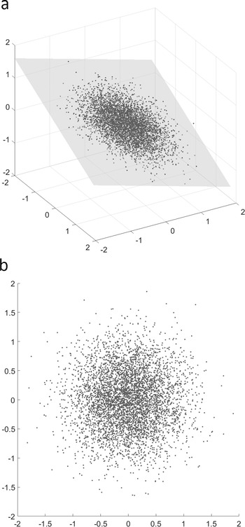
To a close approximation, this is what both PCA and LDA try to do. Returning to the idea of our data set as a cloud of points in our pixel space, we can think of PCA and LDA as techniques for finding informative slices (or cross-sections) of this cloud. Whereas we might think of finding the best angle for making this slice, both techniques assume that we will cut along the first M dimensions of the space and then rotate our coordinate space so that dimensions 1 through N are ordered by informativeness, with the first dimension being the most informative and the last being the least informative. With that completed, it is up to researchers to decide how many of the trailing dimensions to drop (i.e., cut away). If they retain only the first two dimensions, this is akin to selecting the most revealing two-dimensional slice of the cloud (see fig. 1).
a, Samples of data with a disk-like shape and an informative two-dimensional slice of the data. b, Cross-section defined by the slice.

Where PCA and LDA differ is in their criterion of informativeness. PCA defines ‘most informative’ as highest variance. For example, if you wanted to cut a potato into the largest possible chips, you would slice along the longest dimension of the potato as well as the second-longest dimension at right angles to the first. This not only gives you large chips, it gives you the biggest cross-section of the potato and thus a highly informative view of the potato’s internal structure, such as it is. In essence, this is what PCA does. It reorients the data, so that the points are most widely separated along the first dimension, next most widely separated along the second dimension, and so on. Variance is defined as the average distance between each value and the mean value. As such, maximizing variance along a dimension maximizes how much the location of an image along that dimension tells you about how that image differs from the mean image. Figure 1 illustrates the kind of two-dimensional cross-section PCA might recommend for three-dimensional data.
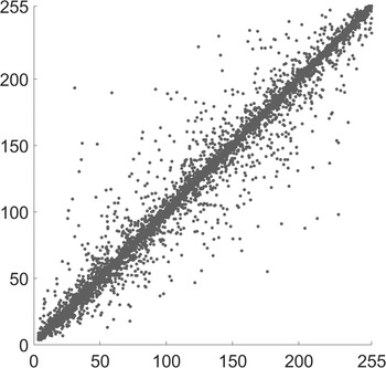
To solidify these concepts, it would be helpful to understand exactly why this approach is at all likely to work in practice. Recall that random images will be uniformly distributed in the pixel space, and any slices you take of it will look pretty much the same. Of course, ordinary images are not random. In particular, the brightness values for individual pixels are highly correlated. For example, if I know the value of one pixel, it is typically a safe bet to guess that neighboring pixels are approximately the same color. This guess will not be perfect, but it is usually much better than guessing the mean color for that pixel across our data set. Luckily, correlations between dimensions (i.e., between the brightness values for different pixels) have the effect of flattening the cloud that represents our data (see fig. 2). This, in turn, means that the cloud affords more informative slices. To appreciate why this flattening is important, consider the difference between a hand and a basketball. Any cross-section you make of the basketball is likely to be roughly equally informative. However, a cross-section of the hand parallel to the palm is much more informative than a cross-section perpendicular to it (either width-wise or lengthwise).
Brightness values for the first two pixels in the first row of the images in the CelebFaces data set (Liu et al. Reference Liu, Luo, Wang and Tang2015).

The numerous correlations between pixels imply a considerable degree of redundancy in the original representation of the image since the brightness values for each pixel carry a lot of information about the brightness of other pixels. In the limit case of perfect correlation, for example, knowing the value of a single variable allows one to perfectly predict the values of the correlated variables. This redundancy is an indicator that image data should be compressible, and as such, we should be able to identify features that represent the images well with less redundancy. To do so, we should aim to identify a few nonredundant dimensions of variation that underlie the highly correlated variables in our original data.Footnote 6 For example, the disk-shaped data shown in figure 1 vary principally along two axes, and the slice defining the cross-section is made along these axes. Given the low variance along the axis orthogonal to the slice, knowing the position of a point along the new axes allows us to make a good guess about the location of any point in the original space.
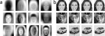
At present, it may be difficult to connect this simple, low-dimensional case to the high-dimensional case involving images. Fortunately, the relevant mathematics makes visualizing the new dimensions easy. Once again, PCA attempts to rotate the coordinate space so that the first dimension is aligned with the direction of highest variance in our data, the second is aligned with the direction of second highest variance (orthogonal to the first), and so on. Geometrically, this operation can be understood as a rotation of the original space. To find the location of our images in this new space, we must rotate those data using a rotation matrix. The details here are not important, but the important thing to know is that each of an image’s coordinates in the rotated space is simply a weighted sum of its original coordinates. Since the original coordinates are pixel brightness values, there is one weight per pixel for each of the new dimensions. We can call these ‘pixel weights’. Rearranging the pixel weights into the shape of an image, we can see how much each new dimension “cares” about each pixel—representing small weights as gray, large positive weights as white, and large negative weights as black (see fig. 3a).
a, First 12 components extracted by PCA using images from the CelebFaces data set. b, Images recovered using a subset of those components. The images on the far left are original. The next three (from left to right) use the first 100, 300, and 500 components, respectively. The cat and car images are taken from the CAT data set (Zhang, Sun, and Tang Reference Zhang, Sun and Tang2008) and Cars data set (Krause et al. Reference Krause, Stark, Deng and Fie-Fie2013), respectively.

Pixels with large weights (either positive or negative) will most affect an image’s coordinate along the new dimension. Conversely, the weighted sum we compute as the value for each dimension tells how relevant that dimension is to reconstructing the image. We can call each set of pixel weights a ‘component’ and these sums ‘component weights’. The component weights (i.e., the new coordinates for each new dimension) tell us how much of each component (literally the pixel weights) must be added to the mean image to recover the original image. Hence, PCA represents images as a weighted sum of components that specifies the difference between each image and the mean image. Since the variance is highest for the earlier components, the magnitude of their component weights will be the greatest on average. Hence, when we drop later components, we will be dropping those dimensions that (on average) capture the smallest deviations from the mean image and retaining those that capture the largest deviations.
This aspect of dimensionality reduction via PCA is important because it illustrates how PCA is a form of compression. PCA identifies the most significant ways that images in our data set differ from the mean image. These “ways” correspond to the components returned by PCA. If we select the first 30 of these components for use as features, we will encode a great deal of information relevant to reconstructing the images while using fewer numbers (i.e., 30 rather than 4,096). Images can be recovered (or “decompressed”) by computing the weighted sum of these components and adding it back to the mean image. Consistent with real patterns, this compression depends on the exploitation of patterns specific to our data set. The components for one data set will not be the same as those for another since the correlations between pixels in each data set will differ. As figure 3b illustrates, when one tries to represent a cat or car image using face components, the fidelity of the recovered images is significantly reduced since face-based components do not capture significant sources of variation in cat or car images. Looking at the components returned by PCA (fig. 3a), it is easy to see why adding them together to produce an image of something other than a face would be difficult.
So far, our exploration of PCA seems promising for the idea that compression is integral to feature extraction. It is easy to see why representing our data in terms of its principal components would facilitate classification since the weights for these components capture the most significant ways our images differ from one another. However, there are strong reasons to think that compression is merely one tool for feature extraction—a tool that is more useful in some contexts than in others.
3.2. Linear Discriminant Analysis
With the essential details of PCA explained, it is easier to understand how LDA differs. Again, both PCA and LDA rotate data so that informative cross-sections of those data can be identified, and both represent images as a weighted sum of components that specify the difference between each image and the mean. Where these techniques differ is in their criterion of informativeness. PCA is an unsupervised technique. That is, it is blind to the categories to which our data belong. In the previous section, I noted that our task was to classify images as belonging to either men or women, but these labels played no role in selecting features via PCA. Unsupervised approaches are useful when we have a lot of unlabeled data since those data need not be discarded when selecting features (Alpaydin Reference Alpaydin2010). However, we do have labels for all 8,000 images used in this case study, and it stands to reason that we might be able to identify better features if we could somehow consider the labels assigned to each image.
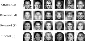
As a supervised technique, LDA does consider these category labels, and (as we will see) LDA extracts better features than PCA for our task. To understand why, we should first get clear on LDA’s criterion of informativeness. Instead of rotating our coordinate space so that the dimensions are prioritized by maximizing variance, LDA prioritizes dimensions by maximizing the ratio of between-category variance to within-category variance. Dimensions fare well under this criterion if the values for items in the same category are similar and the values for items in different categories are dissimilar. Hence, LDA attempts to find dimensions along which the values for images of each category are maximally separable. The effect of this criterion is that the first LDA features tend to emphasize only those aspects of the images that are useful for discriminating between the categories of interest. As figure 4 illustrates, images recovered from the first 30 LDA components exclude many details that are irrelevant to gender identification. For example, things like background color, age, race, eye glasses, and head orientation are lost in the recovered images.
Six pairs of faces. The middle two rows represent the faces as recovered from the top 30 features extracted by LDA.

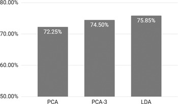
The reader may now begin to see why LDA will not return features that are optimized for compression, but first it is important to establish that LDA can extract better features. Figure 5 compares gender classification results for three sets of features: the first 30 PCA features, the fourth through thirty-fourth PCA features, and the first 30 LDA features. The 2,000 test images classified for this comparison were not among those included in the training set of 8,000 images used to extract the features. Images were classified using a version of the k-nearest neighbors algorithm. For each test image, the algorithm finds the 15 nearest training images in the feature space and guesses the test image’s label on the basis of the distance and labels of these “nearest neighbors” (with closer neighbors getting more of a say).Footnote 7 As we can see, the first 30 PCA features performed worst, the fourth through thirty-fourth PCA features performed better, and the first 30 LDA features performed best. Hence, we can conclude that LDA has identified better features for our task than has PCA.Footnote 8
Classification results for PCA and LDA. PCA-3 images were recovered from the fourth through thirty-fourth PCA features, dropping the first three.

It now remains to be shown that despite their improved performance for classification, LDA features are less optimized for compression than PCA features. The first clue that optimal compression and optimal feature extraction are distinct is that ignoring the first three PCA dimensions improves performance. This is not a novel strategy on my part but a recommendation based on observed performance differences (Belhumeur et al. Reference Belhumeur, Hespanha and Kriegman1997)—differences replicated here. If better compression means better features, it is very surprising that the most informative PCA components can be dropped in order to improve performance. However, if selecting good features is a distinct project with distinct aims, then this need not surprise us.
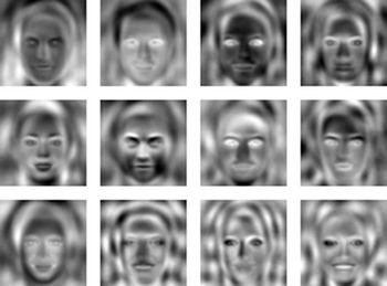
To see how we might explain this result, compare the LDA components shown in figure 6 to the PCA components shown in figure 3. Looking at the earliest components (starting in the top left), the LDA components seem to contain more structural information than the PCA components. The first three PCA components seem to capture a lot of information about the coarse-grained shading of the image. For example, the first PCA component conveys information about foreground/background contrast. This is a very important feature for recovering accurate brightness values for pixels in the image since it tells us about the approximate brightness of large portions of the original image. Nevertheless, it has little to do with identifying the gender of the person in the photo. Learning that the photo is of a fair-skinned person against a dark background does essentially nothing to predict the gender of the subject. In contrast, the information about facial structure captured by the LDA components and later PCA components is more relevant.
First 12 components extracted by LDA. Compare with figure 3a.

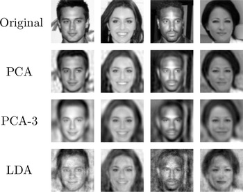
As this suggests, PCA extracts those features that are most relevant to recovering the original image. In practice, this means that the earliest PCA features tend to capture information about large-scale differences in shading, while later dimensions capture finer differences in facial structure. LDA, however, extracts those features that are most relevant to telling men from women. These features also emphasize structural differences but are more narrowly tailored to the task at hand and even less optimized for image reconstruction. As figure 7 shows, the first 100 PCA features easily outperform both the fourth through 104th PCA features and the first 100 LDA features in image reconstruction. Most striking is the fact that as the fidelity of the recovered images drops, classification performance increases. This subjective judgment can be confirmed by common measures of reconstruction error (e.g., Euclidean distance in the pixel space). Hence, it should now be clear that while PCA features are more optimized for compression, they are less optimized for our modeling task.
Four faces recovered from 100 features identified by PCA and LDA. PCA-3 images were recovered from the fourth through 104th PCA features, dropping the first three.

4. Philosophical Lessons
The results reported in the previous section would be surprising if feature extraction were best understood as the process of finding whichever features permit the most accurate and economical reconstruction of the original data (i.e., are most optimized for compression). Nevertheless, the defender of real patterns might argue that descriptive economy still explains why patterns in coarse-grained features reflect patterns in fine-grained data. This argument proceeds as follows:
Even if data scientists do not select features optimized for compression, they nevertheless select features that efficiently encode information about their data. For example, the LDA features efficiently encoded a lot of information about the original data—just not as much as the PCA features. For this reason, we can still say that the LDA features reflect patterns in our data—even if they differ in other ways from features optimized for compression.Footnote 9
There is certainly something right about this idea. In most cases, our features will be of lower dimensionality than our original data and will carry a relatively large amount of information about those data (i.e., they will be efficient). The argument also suggests a helpful distinction between an ontological account of when we should take patterns in a feature seriously and practical considerations about whether that feature is useful for a given task. For example, it would be strange to deny that the first PCA feature represents a real and important dimension of variation in our data just because it is irrelevant to gender classification. Foreground/background contrast really is a major dimension along which our data vary, and the efficiency of that feature seems like a good, task-independent indicator of that fact. Data scientists may have good practical reasons for choosing less efficient features (e.g., LDA features), but the efficiency of these features in absolute terms may best explain why patterns in these features reflect patterns in the original data.
On the contrary, I argue that data scientists’ choices reflect a deeper fact about the relationship between features and data—namely, that the efficiency of a feature is not a good indicator of whether patterns in a feature reflect patterns in our data. To see why, consider the following case. Suppose we are observing a panel of blinking lights arranged in a grid and make note of the states of each light at regular intervals. We notice that the light in the top-left corner turns off and on every second (i.e., 1 second on, 1 second off, etc.). Time series data for this light would be highly compressible since its pattern of illumination is simple and regular. As such, we could reasonably conclude that the light exhibits a pattern—a pattern that is clearly reflected in our original data since the state of the top-left light feature has been selected directly from those data (i.e., our observations).
This much seems obvious, but notice that I said nothing about the behavior of the other lights. Nevertheless, we were able to recognize the pattern in the upper-left light without determining whether the state of the light efficiently encoded any information about the panel as whole. Moreover, the state of the upper-left light seems like a perfectly legitimate feature irrespective of whether the other lights blink in perfect unison with it or whether they blink according to a totally different pattern. In the former case, the state of the upper-left light is a highly efficient feature since we can recover the states of all the other lights once we know its state. In the latter case, the state of the upper-left light is a very inefficient feature since ex hypothesi it tells us little or nothing about the states of the other lights. The primary implication of this case is that efficiency in highly sensitive to the degree of correlation between our features and the variables in our original data. Further, whether any particular data set exhibits such correlations will depend heavily on which variables researchers have chosen to include. For example, if our data only included the states of the first row of lights (which, let’s suppose, blink in unison), the state of the upper-left light could be used to capture the state of the entire row. However, suppose a second row was included, a row that blinks randomly. Should we take the pattern observed in the state of the first light less seriously? Clearly not.
For these reasons, it seems evident that the efficiency of a feature is not what ensures that patterns in that feature reflect patterns in our original data.Footnote 10 This strongly suggests that efficiency is ill suited to explaining how patterns in coarse-grained events reflect patterns in fine-grained events. Perhaps no general explanation of this connection can be given (whether in terms of efficiency or otherwise). In this case, defenders of real patterns may need to rethink the relationship between finer and coarser grains along the lines suggested by Ladyman and Ross (Reference Ladyman and Ross2007, Reference Ladyman, Ross, Ross, Ladyman and Kincaid2013), who reject the claim that coarse-grained patterns are ultimately patterns in fine-grained events. However, it seems too early to conclude that no satisfactory account of this relationship can be given.
Fortunately, there are important feature extraction practices that may offer insights into this relationship. We have seen that feature extraction is concerned with finding features that are useful for a given task, but feature extraction is also concerned with ruling out spurious features. For example, a feature might be contrived to favor a particular hypothesis, introduce misleading artifacts, or encode obscure, coincidental, or idiosyncratic details of our training data. Crucially, patterns in a spurious feature need not reflect any pattern in our data and, more importantly, in the physical events those data describe. By better understanding this fact about spurious features, we might better understand why patterns in good features reflect real patterns in the world.
For example, neural networks are highly flexible feature learning systems, but this flexibility introduces a serious risk that they will merely memorize training data (Arpit et al. Reference Arpit2017). Simplifying for clarity, suppose a particular neuron “fires” whenever a memorized face is seen. The output of such a neuron is a feature of our data to be sure, but compare this neuron to a neuron that responds to differences in facial structure. The activation of either neuron may strongly predict a particular category label, but only in the latter case does this high-level pattern depend on a significant pattern of variation in our original data. Memorizing the fact that a particular image is labeled “woman” is markedly different from learning a relevant type of variation across images. For this reason, constraints are placed on the flexibility of neural networks. For example, researchers might penalize a network for making full use of its connection weights (e.g., by penalizing nonzero weights; Goodfellow, Bengio, and Courville Reference Goodfellow, Bengio and Courville2016), or they might randomly disable particular neurons during training (Arpit et al. Reference Arpit2017). To a first approximation, these constraints force the network to learn features that can be easily and robustly identified.
This suggests that patterns in easily and robustly identifiable features are more likely to reflect patterns in our original data. While this suggestion is intuitively plausible, it is important to get clear on the nature and significance of these virtues. Fortunately, data scientists are keenly interested in offering theoretical motivations for their practices (e.g., in mathematical, geometrical, or information-theoretic terms).Footnote 11 Given their interest in finding patterns in data, understanding how data scientists motivate their criteria for assessing features will likely shed light on why patterns in good features reflect patterns in our original data and, ultimately, in the world those data describe.
To be clear, I am not saying that philosophers can directly read off ontological conclusions from feature extraction algorithms—just as Dennett does not read off his ontological account from image compression algorithms. Instead, Dennett identifies the information-theoretic principles underlying compression algorithms and then explains what these principles have to say about the analogous case of patterns in the world. Similarly, defenders of real patterns might now identify the principles underlying feature extraction and employ these principles to explain how patterns in high-level events relate to patterns in lower-level events. Given the interests of data scientists and the close analogy between features and high-level event descriptions (sec. 2.2), this approach seems highly promising.
5. Conclusion
In this article, I have shown that Dennett’s theoretical motivation for real patterns elides an important aspect of modeling—the identification of useful coarse-grained representations via feature extraction. Further, I have shown that the rationale for real patterns (i.e., the relationship between compression and regularity) cannot be extended to give an account of when patterns in coarse-grained features reflect patterns in our original data. Taken together, this shows that compression alone cannot account for the relationship between high- and low-level models of the world. Crucially, this is not to say that good high-level models fail to capture real patterns in fine-grained events. I believe that they do, but considerations of compressibility can only show that these models capture patterns in coarse-grained events. Connecting these patterns to patterns in fine-grained events is not the project of this article, but the foregoing sections suggest an important direction for future research. Dennett (Reference Dennett1991) attempted to connect two virtues of good models—simplicity and predictive accuracy—to the existence of patterns in the world. Advocates of real patterns might now attempt to complete this picture by connecting patterns in coarse-grained events to patterns in fine-grained events by considering the virtues of good features—especially those concerned with preventing the extraction of spurious features. Fortunately, data science is already in the business of identifying these virtues and has made considerable progress in identifying effective methods of feature extraction. Future work on real patterns would likely benefit from close engagement with data scientific research in this area.