1. INTRODUCTION
Let X = (X1,…, Xn) denote n ≥ 2 jointly distributed real-valued random variables. The order statistics of this set is a reordering of the Xi in terms of nondecreasing values, expressed as X1:n ≤ ··· ≤ Xk:n ≤ ··· ≤ Xn:n. The lowest- and highest-order statistics are denoted by X1:n and Xn:n, respectively. One of the central problems in statistics is to find, bound, or approximate the expected value of order statistics under varying assumptions on the distribution of the random variables. For detailed reviews on this subject, the reader is referred to [9] and [2].
In this article, we focus on finding bounds on the expected value of order statistics under moment information on the random variables. Let X ∼θ m denote the set of feasible distributions θ that satisfies the given moments m for the random variables.
Definition 1: Zk:n* is a tight upper bound on the expected value of the kth-order statistic if

that is, there exists a feasible distribution or a limit of a sequence of feasible distributions that achieves the upper bound.
No other assumptions on independence or the type of distribution are made. In this article, we develop methods to compute Zk:n* under first and second moment information on the random variables. Next, we review some of the classical bounds for order statistics.
1.1. Some Known Bounds
Given identical means and variances (μ,σ2) for the random variables, one of the earliest known bounds for the expected highest-order statistic was derived by Gumbel [10] and Hartley and David [11]. Under the assumption of independence, they obtained the upper bound

. Moriguti [18] extended this result to the special case of symmetrically distributed random variables.
For more general distributions (not necessarily independent or identically distributed), Arnold and Groeneveld [3] obtained an upper bound on the expected value of the kth-order statistic:

Under identical means and variances, this bound reduces to

For this particular case, Arnold and Groeneveld [3] showed that (2) is tight by explicitly constructing a distribution that achieved the bound. However, for general mean–variance information, (1) is not necessarily tight. Aven [4] proposed an alternative upper bound on the expected value of the highest-order statistic:

This bound is also not tight under general mean–variance information. In this article, we develop an algorithmic approach to find (possibly) tight bounds on the expected value of the order statistic Zk:n*. We characterize cases for which the bound can be computed tractably, or we propose simple closed-form bounds that seem promising.
1.2. Contributions
Our main contributions in this article are as follows:
- In Section 2 we find the tight upper bound on the expected value of the highest-order statistic Zn:n* under mean–variance information on the random variables. An efficiently solvable bisection search approach is developed to compute Zn:n*. A discrete extremal distribution is identified that attains the tight bound. Two simple closed-form bounds for the expected highest-order statistic are proposed. Under additional covariance information, we propose a semidefinite programming approach to find the tight bound on the expected highest-order statistic.
- In Section 3 we extend the bisection search method to obtain bounds on the expected value of the general kth-order statistic under mean–variance information. For k < n, we show that the bound is tight under identical means and variances. For general mean–variance information, the bound found with the bisection search method, although not necessarily tight, is at least as strong as (1).
- In Section 4 we provide computational experiments to test the performance of the different bounds.
2. BOUNDS ON EXPECTED HIGHEST-ORDER STATISTIC
We first compute the tight upper bound on the expected highest-order statistic Zn:n* under mean–variance information on the random variables. The mean and variance information on the random variables are denoted as μ = (μ1,…, μn) and σ2 = (σ12,…, σn2). The set of feasible distributions satisfying these moment restrictions is represented by X ∼θ (μ, σ2). For simplicity of presentation, we will assume that all of the σi are strictly positive. As discussed later, this condition can in fact be relaxed.
The approach to compute the tight upper bound on the expected value of the highest-order statistic is based on a convex reformulation technique, initially proposed by Meilijson and Nadas [17] and developed later in Bertsimas, Natarajan, and Teo [5]. The reformulation is based on the observation that the highest-order statistic Xn:n is a convex function in the Xi variables. We review the key ideas of this reformulation next.
Theorem 1 (Bertsimas et al. [5]): The tight upper bound on the expected value of the highest-order statistic Zn:n* given X ∼θ (μ, σ2) is obtained by solving

where x+ = max(0,x).
Sketch of Proof: We first show that (4) provides an upper bound on Zn:n*. To see this, note that we have the following inequality for each variable Xi:

Since the right-hand side of this inequality is independent of the particular i, we have

Taking expectations and minimizing over the zi variables, we obtain the best upper bound:

Optimizing over distributions with given mean–variance information, we obtain an upper bound:

Note that the inner problem is optimization over probability distributions of single random variables θi, since no cross-moment information is specified. For a proof that the bound is tight, the reader is referred to [5]. Alternatively, we construct an extremal distribution in Theorem 3 that attains the bound. █
The solution for the inner problem in (4) is in fact known in closed form from [13] and [22]. We now outline a simple proof for this bound.
Proposition 1: The tight upper bound on the expected value Eθi [Xi − zi]+ given Xi ∼θi (μi,σi2) is

Proof: We have the basic equality

Taking expectations, we obtain

Furthermore, this bound can be shown to be tight since it is attained by the distribution

Using this closed-form bound, we now show that the tight upper bound on the expected highest-order statistic can be found by solving a univariate convex minimization problem.
Theorem 2: The tight upper bound on the expected value of the highest-order statistic Zn:n* given X ∼θ (μ, σ2) is obtained by solving the strictly convex univariate minimization problem

Proof: Combining Theorem 1 and Proposition 1, the tight upper bound on the expected highest-order statistic is

We next show that (7) can be simplified to a single-variable optimization problem. Let z* be an optimal solution to (7) and let zn:n* denote the highest-order statistic. Note that the second term,

, is decreasing in zi. Hence, for any i < n with zi:n* < zn:n*, by increasing zi:n* up to zn:n* the first term remains unaffected while the second term decreases, thus reducing the objective. Since we are minimizing the objective, the optimal solution will set all of the zi* values equal to zn:n*. █
It can be easily checked that fn:n is a strictly convex function, implying that the function has a unique global minimum. The optimal decision variable z* in (6) hence satisfies the first-order condition obtained by setting the derivative ∂fn:n(z)/∂z to zero:

Remark: Our result can be viewed as an extension of the bound from Lai and Robbins [15] and Ross [21]. In their case, under completely known marginal distributions Xi ∼θ θi, they obtain the following tight bound on the highest-order statistic:

Note that this result follows also from Meilijson and Nadas [17].
2.1. An Extremal Probability Distribution
We construct an n-atom discrete distribution that satisfies that mean–variance requirements and attains the bound in (6).
Theorem 3: Let z* denote the optimal minimizer to (6). An n-atom extremal distribution for X that achieves the upper bound and satisfies the mean–variance requirements is

where X(j) = (X1(j),…, Xn(j)) is expressed as

Proof: From the definition, it is clear that the pj values denote a probability measure since pj ≥ 0 for all j and

It can be verified for this n-atom distribution that

Furthermore, the maximum among the n random variables for the jth atom is attained by Xj(j). Thus,

This n-atom distribution attains the upper bound on the expected value of the highest-order statistic and satisfies the mean and variance requirements. This verifies that the bound in Theorem 1 is tight. █
2.2. Solution Techniques
In general, it does not seem possible to find Zn:n* in closed form. A special case under which this is possible is discussed next.
2.2.1. Identical Mean and Variance
For identical mean–variance pairs (μ,σ2), solving (8) yields the optimal value for z*:

Substituting this into (6) yields the tight bound

Note that this is exactly (2) obtained by Arnold and Groeneveld [3] for k = n. A distribution that attains this bound is randomly selecting n elements without replacement from the set in which one element has the value
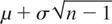
and the remaining n − 1 elements have the value

.
2.2.2. General Mean–Variance Pairs
For the general case, we outline a simple bisection search algorithm to find Zn:n*.
Description of the Algorithm
1. Initialize zl and zu such that ∂fn:n(zl)/∂z ≤ 0 and ∂fn:n(zu)/∂z ≥ 0 and ε > 0 to a given tolerance level.
2. Let z = (zl + zu)/2.
3. While |∂fn:n(z)/∂z| ≥ ε, do:
(a) If ∂fn:n(z)/∂z ≥ 0, set zu = z; or else set zl = z.
(b) Go back to Step 2.
4. Output Zn:n* = fn:n(z).
We propose two simple upper and lower bounds zu and zl on the range of the optimal z* to initialize the algorithm. Consider the problem of finding a zu such that f′(zu) ≥ 0. One such zu is constructed such that each term on the left-hand side of (8) contributes at least a fraction (n − 2)/n:

which reduces to

We choose zu as

Similarly, a lower bound zl can be found such that

A zl that satisfies this condition is

Our computational tests indicate that these values of zu and zl lead quickly to the tight bound.
2.2.3. New Closed-Form Bounds
Based on the two end points, we now propose simple closed-form bounds on the expected value of the highest-order statistic.
Theorem 4: Two closed-form upper bounds on the expected value of the highest-order statistic given X ∼θ (μ, σ2) are


Proof: Substitute z = zl and z = zu in (6) respectively. █
Note that (13) and (14) reduce to the tight upper bound (10) on the expected highest-order statistic for random variables with identical mean–variance pairs.
2.3. Extensions
We now extend the results to the case where some of the σi2 = 0 (i.e., Xi is deterministic). Without loss of generality, we assume that exactly one variable is deterministic since the case with multiple constants can be reduced to this case by choosing the maximum of the constants. Given n ≥ 1 random variables with strictly positive variances and a constant K, we want to find the tight upper bound on Eθ [max(Xn:n,K)]. By introducing an extra decision variable, zn+1, for the term K, (4) reduces to

Using an argument similar to Theorem 2, it can be checked that the optimal solution will set all of the zi values the same at a value greater than or equal to K. Hence, the tight upper bound on the expected highest-order statistic is

which reduces to the constrained version of (6):

The tight upper bound can be found by a modified bisection search method:
- Solve the unconstrained version of (16) with bisection search to find z*.
- Output fn:n(max(z*,K)).
We propose using the following two closed-form bounds in this case:

and

2.4. Extensions to Additional Covariance Information
In this subsection, we propose an algorithmic approach to find the tight upper bound on the expected value of the highest-order statistic under covariance information. Given the mean and covariance matrix for the random variables X ∼θ (μ,Q), the tight upper bound is computed by finding a distribution θ that solves

Here

if

and zero otherwise represents the indicator function. This problem has been well studied under the class of moment problems in Isii [12] and Karlin and Studden [14]. To solve (19), we construct the dual problem by introducing variables y, Y, and y0 for each of the moment constraints. The dual problem is formulated as

The constraints in (20) imply the nonnegativity of a quadratic function over

. By taking the expectation of the dual constraints, it is easy to see that Z* ≥ Zn:n*. Furthermore, Isii [12] showed that if the covariance matrix Q [sc ] 0 is strictly positive definite, then Z* = Zn:n*. Under this assumption, the convexity of Xn:n implies that the tight upper bound on the expected highest-order statistic is

Let e(i) denote a unit vector with the ith component ei(i) = 1 and zero otherwise. The equivalence between the global nonnegativity of a quadratic polynomial and the semidefinite representation [20] implies that (21) can be rewritten as

Here A [sccue ] 0 denotes the constraint that the matrix A is positive semidefinite. Formulation (22) is a semidefinite optimization problem that can be solved within ε > 0 of the optimal solution in polynomial time in the problem data and log(1/ε) [19]. In practice, standard semidefinite optimization codes such as SeDuMi [23] can be used to find the tight upper bound on the expected highest-order statistic under covariance information.
3. BOUNDS ON EXPECTED kTH-ORDER STATISTIC
In this section, we generalize our results to find bounds on the expected value of the kth-order statistic for k < n under mean–variance information on the random variables; that is,

Our results are based on the simple observation that

We find tight bounds on the expected value of the right-hand side of (23) to obtain bounds on the expected value of the kth-order statistic.
Theorem 5: The tight upper bound on the expected value of the sum of the kth- to nth-order statistic given X ∼θ (μ, σ2) is obtained by solving

Proof: Using the result from Bertsimas et al. [5], the upper bound on the sum of the expected value of the kth- to nth-order statistic is

As earlier, (25) can be reduced to a single-variable optimization problem. To see this, let z* be an optimal solution to (25). For any l < k with zl:n* < zk:n*, we can increase zl:n* to zk:n* since the first term is unaffected (

is unaffected by change in zl:n*, for l < k, provided zl:n* < zk:n*) while the second term decreases in zl:n*. Hence, we have zl:n* = zk:n* for l < k. Furthermore, for l > k with zl:n* > zk:n*, by decreasing zl:n* to zk:n* the first term decreases at a rate of 1 while the second term increases at a rate of at most 1. Since we want to minimize our objective, we have zl:n* = zk:n* for l = 1,…, n. █
Using (23) and Theorem 5, we now obtain a bound on the expected kth-order statistic.
Theorem 6: An upper bound on the expected value of the kth-order statistic Zk:n* given X ∼θ (μ, σ2) is obtained by solving

Note that the nonconvex structure of the kth-order statistic for k < n implies that (26) is not necessarily tight for general mean–variance pairs. However, (26) is at least as tight as (1) proposed by Arnold and Groeneveld [3]. This follows from observing that they obtained their bound by bounding (23), although not in the tightest manner. A special case under which (26) is tight is described next.
3.1. Identical Mean and Variance
For identical mean–variance pairs (μ,σ2), (26) yields the optimal value for z*:

Substituting this into (26) yields

This is exactly (2) obtained by Arnold and Groeneveld [3]. To see that (27) is tight, consider a distribution obtained by randomly selecting n elements without replacement from the set in which n − k + 1 elements have the value

and the remaining k − 1 elements have the value

. It is easy to verify that this distribution attains the bound as described earlier.
3.2. General Mean-Variance Pairs
For the general case, we propose the use of the bisection search algorithm to find the bound on the expected kth-order statistic by solving minz fk:n(z). The lower and upper bounds on the range of the optimal z* to initialize the bisection search method in this case reduces to

and

Theorem 7: Two closed form upper bounds on the expected value of the kth-order statistic given X ∼θ (μ, σ2) are


4. COMPUTATIONAL RESULTS
In this section, we evaluate the quality of the various bounds proposed in this article. The first example is an application of the highest-order statistic bound in a financial context. The second example is a simulation experiment to compare the performance of the bounds for the general kth-order statistic. The computations were conducted on a Pentium II (550 MHz) Windows 2000 platform with the total computational time under a minute.
4.1. Application in Option Pricing
One of the central questions in financial economics is to find the price of a derivative security given information on the underlying assets. Under a geometric Brownian motion assumption on the prices of the underlying assets and using the no-arbitrage assumption, the Black–Scholes [7] formula provides an insightful answer to this question. Assuming no arbitrage, but without making specific distributional assumptions, Lo [16], Bertsimas and Popescu [6], and Boyle and Lin [8] derived moment bounds on the prices of options. Our particular focus is on finding bounds on the price of an option known as the lookback option under moment information on the asset prices.
Let x1,x2,…, xn denote the price of an asset at n different times. A simple lookback European call option on these assets with strike price K ≥ 0 has a payoff of max(Xn:n − K,0). Let r denote the risk-free interest rate and T denote the maturity date. Under the no-arbitrage assumption, the price of the lookback option is

where the expectation is taken over the martingale measure. Clearly, the price of this option depends on the highest-order statistic. Under mean and variance information on Xi, Boyle and Lin [8] proposed the following upper bound on the price of the lookback option:

We use the results from Section 2 to find the best bounds on P(K). Note that although the asset prices are nonnegative in practice, we do not model this explicitly here to compute our bounds.
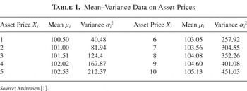
The specific lookback option-pricing example is taken from Andreasen [1]. An upper bound on the price of a European call lookback option over n = 10 time steps is calculated. The risk-free interest rate (r) is 5% and the time to maturity (T) is 1 year. Table 1 provides the mean and variance information of the asset prices over the 10 periods.
Mean–Variance Data on Asset Prices

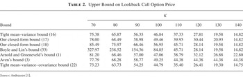
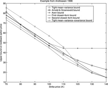
The bounds on the option price are computed for strike prices K from 70 to 140 in steps of 10. Table 2 provides six bounds under mean–variance information and an additional bound under covariance information. For the last bound, we assumed that the asset prices were uncorrelated and solved (22) with the semidefinite optimization code SeDuMi. From Table 2, it is observed that Boyle and Lin's bound is very loose for small values of K. On average, our proposed closed-form bound (17) outperforms both Arnold and Groeneveld's [3] and Aven's [4] bound, respectively. Although the closed-form bound (18) is weaker for smaller K, it is in fact tight for larger K, indicating its usefulness. In Figure 1, we provide the graphical comparison of the bounds (excluding Boyle and Lin's [8] bound, which is tight only for large K).
Upper Bound on Lookback Call Option Price


Upper bound on lookback call option price. From Andreasen [1].
4.2. Simulation Test
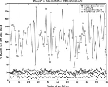
The second example is a simulation test to compare the relative performance of the different bounds under randomly generated moment information. We consider n = 30 random variables. The mean–variance pairs for each random variable were independently chosen from a uniform distribution with μi ∼ U [0, 50] and σi2 ∼ U [100,400]. One hundred mean–variance pairs were sampled in these ranges and the bounds on the expected order statistics were computed. For each closed-form bound, we evaluate the relative percentage error:

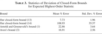
For the highest-order statistic, the percentage error of the bounds are provided in Figure 2 and Table 3.

Deviation of closed-form bounds from tight bound on expected highest-order statistic.
Statistics of Deviation of Closed-Form Bounds for Expected Highest-Order Statistic

Note that in this case, the bisection search method finds the tight bound Zn:n*. In this case, our closed-form bound (13) performs the best and bound (14) is relatively weaker.
We next consider the results for a lower-order statistic. Since the upper bound for the lowest-order statistic Z1:n* from (23) simply reduces to

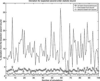
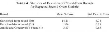
, we use the second lowest-order statistic Z2:n* to compare the bounds. For this case, the bisection search method does not guarantee finding the tight bound. The results obtained are presented in Figure 3 and Table 4. For this case, our closed-form bound (14) is observed to be tightest among the closed-form bounds, with an average percentage error of about 1%.

Deviation of closed-form bounds from bisection bound on second-order statistic.
Statistics of Deviation of Closed-Form Bounds for Expected Second-Order Statistic

The simulation results seem to indicate that the two closed-form bounds perform well in reasonable settings. Interestingly, in each of the two simulations, the best-closed form bounds were observed to be one of our bounds. Although cases can be constructed for which both of the bounds are weaker than either Arnold and Groeneveld's and Aven's bounds, the results suggest that the bounds are useful.
5. SUMMARY
In this article, we studied the problem of finding tight bounds on the expected value of order statistics under first and second moment information on the random variables. For the highest-order statistic, we showed that the tight upper bound could be found efficiently under mean–variance information with a bisection search method and under mean–variance–covariance information with semidefinite programming. For the general kth-order statistic, we provided efficiently computable bounds (not necessarily tight) under mean–variance information. Finding tight bounds for the general kth-order statistic under mean–variance and possibly covariance information is a potential research area for the future.
Acknowledgment
This research was supported in part by the Singapore–MIT alliance.