1. Introduction
Magnetic reconnection is a change of topology of the magnetic field lines taking place in regions of intense localised current, referred to as current sheets. This fundamental process ultimately converts magnetic energy into bulk flow and particle heating, and is responsible for the explosive release of magnetic energy in astrophysical and laboratory plasmas. The instabilities of very elongated reconnecting current sheets leading to the formation of secondary magnetic islands, called plasmoids, have generated a lot of interest, as they are believed to achieve fast reconnection. Plasmoids have been thoroughly studied through the most standard reconnection model based on the Sweet–Parker (SP) theory in the resistive magnetohydrodynamics (RMHD) framework (Biskamp Reference Biskamp1986; Loureiro et al. Reference Loureiro, Cowley, Dorland, Haines and Schekochihin2005). In Biskamp (Reference Biskamp1986), it has been shown that collisional current sheets become unstable above a critical Lundquist number $S= \mu _0 L_{\rm sp} v_A /\eta > S_c = 10^4$ , where $L_{\rm sp}$
 is the length of the SP current sheet, $\eta$
 is the resistivity and $v_A$
 is the Alfvèn speed. Much work has followed and allowed to identify the plasmoid regime as a function of the Lundquist number and of the characteristic scale of a dynamic of the ions (ion-sound Larmor radius $\rho _s$
 or ion skin depth $d_i$
 scales) at which a transition to a non-collisional regime, dominated by kinetic effects, occurs (Uzdensky, Loureiro & Schekochihin Reference Uzdensky, Loureiro and Schekochihin2010a,Reference Uzdensky, Loureiro and Schekochihinb; Ji & Daughton Reference Ji and Daughton2011; Daughton & Roytershteyn Reference Daughton and Roytershteyn2012; Loureiro & Uzdensky Reference Loureiro and Uzdensky2015; Bhat & Loureiro Reference Bhat and Loureiro2018). This extension of the resistive reconnection regime with the inclusion of the ion dynamics enlarged the study to a broader parameter space, but also suggested that plasmoids are fundamental features of reconnecting current sheets, regardless of the value of the Lundquist number (Ji & Daughton Reference Ji and Daughton2011; Daughton & Roytershteyn Reference Daughton and Roytershteyn2012).
The plasma in the magnetosphere and solar wind, which regularly undergoes reconnection, is so dilute that collisions between particles are extremely infrequent. In such plasmas, electron inertia becomes particularly relevant to drive reconnection in thin current sheets. Indeed, recent observations revealed many reconnection onsets driven by electrons, in the presence of a strong guide field, close to the dayside magnetopause and magnetosheath (Burch et al. Reference Burch, Torbert, Phan, Chen, Moore, Ergun, Eastwood, Gershman, Cassak and Argall2016; Phan et al. Reference Phan, Eastwood, Shay, Drake, Sonnerup, Fujimoto, Cassak, Oieroset, Burch and Torbert2018) with current sheets having a thickness of the order of the electron inertial length. Regarding experiments, a study by Olson et al. (Reference Olson, Egedal, Greess, Myers, Clark, Endrizzi, Flanagan, Milhone, Peterson and Wallace2016) also gave direct experimental proof of plasmoid formation at the electron scale in a weakly collisional regime. In these collisionless, magnetised environments, effects of the finite electron Larmor radius (FLR) on the reconnection process can also become non-negligible, in particular when $\beta _e$ , defined as the ratio between equilibrium thermal electron pressure and guide field magnetic pressure, is not much smaller than unity. Although the plasma-$\beta$
 effect was found to have an effect on the plasmoid instability threshold in the collisional regime (Ni et al. Reference Ni, Ziegler, Huang, Lin and Mei2012) and in the semi-collisional regime (Baty Reference Baty2014), it has been ignored in most collisionless studies. This motivates the study of the formation of plasmoids in non-collisional current sheets and, in particular, of the effects relevant at the electron scales such as the electron skin depth and the electron Larmor radius.
In Granier et al. (Reference Granier, Borgogno, Comisso, Grasso, Tassi and Numata2022a), the purely collisionless plasmoid regime was investigated in the regime of strong guide field with $\beta _e \rightarrow 0$ . The instability was studied in a phase space defined by two kinetic scales, $d_e$
 (electron inertial length) and $\rho _s$
 (the ion-sound Larmor radius), compared with the current sheet length $L_{{\rm cs}}$
 . In a first regime, where the ion-sound Larmor radius is much smaller than the thickness of the boundary layer, $\rho _s \ll \delta _{\rm in}$
 , plasmoids were obtained for current sheets having a critical aspect ratio $A_\star ^{(1)} = (L_{{\rm cs}}/\delta _{{\rm cs}}) \sim (L_{{\rm cs}}/d_e) \sim 10$
 . In a second regime, where the ion-sound Larmor radius is of the order of, or larger than, the thickness of the inner region, the critical aspect ration can be below $10$
 and was found to scale as $A_\star ^{(2)} \propto L_{{\rm cs}}/\rho _s$
 . In the present work, we relax the assumption of small $\beta _e$
 and carry out a detailed study of the effect of a finite $\beta _e$
 , on the collisionless plasmoid instability, in the case of a strong guide field. We consider inertial reconnection, and finite electron FLR effects arise from the combination of electron inertia and finite $\beta _e$
 parameters. This study is conducted through a comparison of gyrofluid and gyrokinetic simulations. Previously, the gyrokinetic method was successfully employed to examine reconnection (Pueschel et al. Reference Pueschel, Jenko, Told and Büchner2011; Zocco & Schekochihin Reference Zocco and Schekochihin2011; Zacharias et al. Reference Zacharias, Comisso, Grasso, Kleiber, Borchardt and Hatzky2014; Numata & Loureiro Reference Numata and Loureiro2015; Rogers et al. Reference Rogers, Kobayashi, Ricci, Dorland, Drake and Tatsuno2007). Both approaches are assuming that the plasma is immersed in a strong guide field oriented along the $z$
 direction. As a by-product of our analysis, we also obtain a way to validate, by means of gyrokinetic simulations, part of the results on collisionless plasmoid instability obtained by Granier et al. (Reference Granier, Borgogno, Comisso, Grasso, Tassi and Numata2022a) with a gyrofluid approach in the $\beta _e \rightarrow 0$
 limit (later referred to as the fluid limit).
The adopted gyrofluid model is the 2-field system presented in Granier et al. (Reference Granier, Borgogno, Grasso and Tassi2022b) and assumes cold and immobile ions along the guide field direction. Gyrofluid models, although greatly simplified with respect to the original gyrokinetic system, are useful tools for studying collisionless reconnection, in which the microscopic scales, such as the electron skin depth and the electron Larmor radius, can be more important than resistivity. In addition, the gyrofluid framework is less costly in terms of computational resources, and physically more intuitive when compared with the kinetic or gyrokinetic framework. So far, gyrofluid modelling has allowed us to gain a good understanding of the role of collisionless effects (e.g. Del Sarto et al. Reference Del Sarto, Marchetto, Pegoraro and Califano2011; Comisso et al. Reference Comisso, Grasso, Waelbroeck and Borgogno2013; Tassi et al. Reference Tassi, Grasso, Borgogno, Passot and Sulem2018; Granier et al. Reference Granier, Tassi, Borgogno and Grasso2021, Reference Granier, Borgogno, Grasso and Tassi2022b).
The gyrokinetic model, adopted for the comparison, is a $\delta f$ model which solves the electromagnetic gyrokinetic Vlasov–Maxwell system. The gyrokinetic equations are solved by means of the AstroGK code, presented and used in Numata et al. (Reference Numata, Howes, Tatsuno, Barnes and Dorland2010); Numata & Loureiro (Reference Numata and Loureiro2015). One of the main advantages of using the AstroGK code for a comparison with the gyrofluid results, is that, in a specific limit, the gyrokinetic system solved by AstroGK reduces to the one that was taken to derive the 2-field gyrofluid model used in this study (Howes et al. Reference Howes, Cowley, Dorland, Hammett, Quataert and Schekochihin2006). This allows us to study the effect of the closure applied on the moments, performed during the derivation of the gyrofluid model, on the distribution and conversion of energy during reconnection, and identify the possible limitations of the gyrofluid approach. The specific limit in which the AstroGK code has to be used, in order to reproduce the parent gyrokinetic model of the gyrofluid model, is that corresponding to a straight guide field, with no density and temperature gradients and without collisions. To be consistent with the gyrofluid approach, the ions are assumed to be cold.
The article is organised as follows. In § 2 we present the gyrofluid and gyrokinetic systems, as well as the numerical set-up. In § 3 we present the results concerning the plasmoid instability obtained from a comparison of the two approaches. In § 4 we compare the energy variations in the two frameworks and discuss the effect of the closure hypothesis on the energy conversion. Section 5 is devoted to conclusions.
2. Adopted models
2.1. Gyrofluid
The gyrofluid model used for our analysis is that considered by Granier et al. (Reference Granier, Borgogno, Grasso and Tassi2022b), which consists of the following evolution equations


complemented by the relations


Equation (2.1) corresponds to the electron gyrocentre continuity equation, whereas (2.2) refers to the electron momentum conservation law, along the guide field direction. The static relations (2.3)–(2.5) descend from quasi-neutrality and from the projections of Ampère's law along directions parallel and perpendicular to the guide field, respectively. As mentioned previously, the guide field is directed along the $z$ axis of a Cartesian coordinate system $x,y,z$
 , and, in the present two-dimensional (2D) version of the model, the dependent variables are functions only of $x$
 and $y$
 , as well as of the time variable $t$
 . We indicated with $N_e$
 and $U_e$
 the fluctuations of the electron gyrocentre density and parallel velocity, respectively, whereas $\phi$
 and $B_\parallel$
 indicate the fluctuations of the electrostatic potential and of the magnetic field along the guide field. The variable $A_e$
 is defined by $A_e=G_{10e} A_{\parallel } - d_e^2 U_e$
 , where $A_{\parallel }$
 is the $z$
 -component of the magnetic vector potential, $d_e=\sqrt {m_e c^2/{4 {\rm \pi}e^2 n_0}}/L$
 is the normalised electron skin depth and $G_{10e}$
 is an electron gyroaverage operator, defined later in (2.10). The operator $[ \, , \, ]$
 is the canonical Poisson bracket and is defined by $[f,g]=\partial _x f \partial _y g - \partial _y f \partial _x g$
 , for two functions $f$
 and $g$
 . The perpendicular Laplacian operator $\nabla _{\perp }^2$
 is defined by $\nabla _{\perp }^2 f=\partial _{xx}f + \partial _{yy} f$
 . The variables are normalised as


where the hat indicates dimensional variables, $c$ is the speed of light, $L$
 is a characteristic scale length, $n_0$
 is the equilibrium uniform density, $B_0$
 is the amplitude of the guide field and $v_A=B_0/\sqrt {4 {\rm \pi}m_i n_0}$
 is the Alfvén speed, with $m_i$
 indicating the ion mass. The normalised ion skin depth is defined by $d_i=\sqrt {m_i c^2/{4 {\rm \pi}e^2 n_0}}/L$
 , where $e$
 indicates the proton charge. In (2.7a,b) we also introduced the quantities $N_i$
 and $U_i$
 , corresponding to the ion gyrocentre density and parallel velocity fluctuations, respectively. Such moments do not evolve in the model (2.1)–(2.5), and the assumptions on such quantities are discussed later in this section, as well as in § 4. We find it also useful to write explicitly the expression for the magnetic field normalised with respect to the guide field amplitude. In the present 2D setting, by virtue of the normalisation (2.6a–c)–(2.8a–c), such expression is given by

where $\boldsymbol {z}$ is the unit vector along $z$
 . Independent parameters in the model are $\beta _e=8 {\rm \pi}n_0 T_{0e}/B_0^2$
 , $\rho _s=\sqrt {{T_{0e} m_i c^2}/{(e^2 B_{0}^2)}}/L$
 and $d_e$
 .Footnote 1 These three parameters correspond to the ratio between equilibrium electron pressure and magnetic guide field pressure, to the normalised sonic Larmor radius and to the electron skin depth, respectively.
The model is formulated on a domain $\{ (x,y) : -L_x \leq x \leq L_x , -L_y \leq y \leq L_y \}$ , with $L_x$
 and $L_y$
 positive constants. Periodic boundary conditions are assumed. This allows to express gyroaverage operators in terms of the corresponding Fourier multipliers. In particular, we associate the electron gyroaverage operators $G_{10e}$
 and $G_{20e}$
 with corresponding Fourier multipliers in the following way (Brizard Reference Brizard1992)

where $k_{\perp }^2=k_x^2 + k_y^2$ is the squared perpendicular wave number and $k_x=m {\rm \pi}/L_x$
 , $k_y=n {\rm \pi}/L_y$
 are the $x$
 and $y$
 components of the wave vector, with $m$
 and $n$
 positive integers. As is customary with gyrofluid models, (2.1) and (2.2) are expressed in terms of gyrocentre variables. However, for the sake of the subsequent analysis, it can be useful also to express their relation with particle variables. Such relation, in particular, is affected by the quasi-static assumption, used in the derivation of the model (Tassi, Passot & Sulem Reference Tassi, Passot and Sulem2020) to obtain a closure on the infinite hierarchy of moment equations obtained from a parent gyrokinetic system. As a consequence of such quasi-static closure (which are briefly recalled in § 4) the normalised density fluctuations and parallel velocity fluctuations of the electrons, indicated with $n_e$
 and $u_e$
 , respectively, are related to those of the corresponding gyrocentres by


In addition, in our gyrofluid model we neglect the contributions due to the density and parallel velocity fluctuations of the ion gyrocentres, by imposing that $N_i=0$ , $U_i=0$
 . Furthermore, ions are assumed to be cold, i.e. $\tau \rightarrow 0$
 , where $\tau =T_{0i}/T_{0e}$
 is the ratio between ion and electron equilibrium temperature.
In terms of the ion particle density and parallel velocity fluctuations, denoted as $n_i$ and $u_i$
 , respectively, such assumptions lead to the relations $n_i= \nabla _{\perp }^2 \phi + B_\parallel = n_e$
 and $u_i=0$
 . From the quasi-neutrality relation (2.3), Ampère's law (2.4) and (2.5), combined with (2.11) and (2.12), we can obtain the relations


that permit to express the electron particle (as opposed to gyrocentre) density and parallel velocity fluctuations, in terms of electromagnetic perturbations such as $\phi$ , $B_\parallel$
 and $A_{\parallel }$
 .
It is also particularly relevant to consider the limit $\beta _e \rightarrow 0$ with $d_e$
 and $\rho _s$
 remaining finite (which implies $m_e /m_i \rightarrow 0$
 ). This corresponds to suppressing the effects of parallel magnetic perturbations and electron FLR effects. One of the purposes of our investigation is indeed to consider possible modifications, due to kinetic effects, of the plasmoid instability scenario described by Granier et al. (Reference Granier, Borgogno, Comisso, Grasso, Tassi and Numata2022a) and which was conceived namely in the regime with $\beta _e \rightarrow 0$
 and finite $d_e$
 and $\rho _s$
 . In this limit, the gyroaverage operators can be approximated in the Fourier space in the following way:

Using this development in (2.1)–(2.5) and neglecting the first-order corrections, we obtain the evolution equations (Schep, Pegoraro & Kuvshinov Reference Schep, Pegoraro and Kuvshinov1994)


where the static relations (2.3)–(2.5) are replaced by


In this limit, particle density and parallel velocity fluctuations coincide with the corresponding gyrocentre counterparts. The system (2.16) and (2.17), complemented by the static relations (2.18) and (2.19) corresponds to the model by Cafaro et al. (Reference Cafaro, Grasso, Pegoraro, Porcelli and Saluzzi1998), adopted for describing collisionless reconnection in the presence of electron inertia and finite sonic Larmor radius effects. Because of the absence of FLR effects, we refer to the model (2.16)–(2.19) as to the fluid limit of the general gyrofluid model (2.1)–(2.5). This model was used extensively for studying reconnection in the past, and a dispersion relation was derived in Porcelli (Reference Porcelli1991).
We point out that it is possible to take the small FLR limit of (2.2), with parameters satisfying ($d_e \ll 1$ , $\rho _s \ll 1,$
 $d_e/\rho _s \ll 1$
 , $\beta _e = O(1))$
 and $\nabla _{\perp }^2 = O(1)$
 , to obtain an Ohm's law given by

This equation retains first-order corrections proportional to $(\beta _e/4)d_e^2$ and $\beta _e\rho _s^2/(2+\beta _e)$
 , that arise from both electron FLR (assuming $G_{10e} \approx 1 +(\beta _e/4)d_e^2 \nabla _\perp ^2$
 for $d_e \ll 1$
 ) and finite $B_\parallel$
 effects, respectively. The dispersion relation of Porcelli (Reference Porcelli1991), which was obtained by adopting boundary layer and asymptotic matching techniques for $\beta _e=0$
 , can be extended by identifying an effective electron skin depth $d_e'$
 and effective sonic Larmor radius $\rho _s'$
 , given by $d_e'/d_e = \sqrt {1 - \beta _e/4}$
 and $\rho _s'/\rho _s=\sqrt {2/(\beta _e +2})$
 , respectively. This assumes that one can perform the matching asymptotic expansion as in the case without electron FLR effects, apart from the correction embedded in $d_e '$
 . This excludes, in particular, the role played, in the dispersion relation, by a possible innermost boundary layer of size proportional to some positive power of $\beta _e$
 . However, as shown in figure 1, the comparison with numerical simulations suggests that, at least for the small values of $\beta _e$
 considered, such approximation, appears to describe effectively the dependence on $\beta _e$
 of the linear growth rate.
Evolution of linear growth rate as a function of $k_y$ for $d_e = 0.085$
 , $\rho _s = 0.3$
 . For $\beta _e = 0$
 , the solution corresponds to that of Porcelli (Reference Porcelli1991), while the cases $\beta _e = 0.12$
 and $\beta _e = 0.24$
 represent an extension of this solution accounting for small electronic FLR effects and parallel magnetic perturbations.

2.2. Gyrokinetic
In this section, we present the electromagnetic $\delta f$ gyrokinetic model used in this work (Howes et al. Reference Howes, Cowley, Dorland, Hammett, Quataert and Schekochihin2006; Numata et al. Reference Numata, Howes, Tatsuno, Barnes and Dorland2010), from which the gyrofluid model can be derived with appropriate approximations and closure hypotheses (Tassi et al. Reference Tassi, Passot and Sulem2020). The gyrokinetic model is formulated in terms of the perturbation of the gyrocentre distribution function $g_s = g_s(\textbf {X}_s, v_{\parallel }, v_\perp, t)$
 where $v_{\parallel }$
 , $v_\perp$
 are the parallel and perpendicular velocity coordinates. The guiding centre coordinates are given by

where $\boldsymbol {x}$ is the particle position, $\boldsymbol {v}$
 is the particle velocity, $v_{{\rm th}_s}=\sqrt {T_{0s}/m_s}$
 is the thermal speed and $\omega _{cs}=e B_0 /(m_s c)$
 is the cyclotron frequency. The index $s$
 labels the particle species, with $s=e$
 for electrons and $s=i$
 for ions. For simplicity, we assume a uniform background plasma, and two-dimensionality ($\partial /\partial z = 0)$
 . By adopting the same normalisation scheme with the gyrofluid model, the gyrokinetic system can be written in the following way:


Equation (2.23) is the gyrokinetic equation, whereas (2.24)–(2.26) correspond to the quasi-neutrality relation and to the parallel and perpendicular projection of Ampère's law. We have introduced the following additional normalisations

where the Maxwellian equilibrium distribution function in the dimensional form is

The species-dependent parameters are the mass ratio $\sigma _s = m_s/m_i$ , temperature ratio $\tau _s = T_{0s}/T_{0e}$
 and charge number ratio $Z_s = q_s/q_i$
 . Obviously, $\sigma _i=1$
 , $\tau _e = 1$
 , $Z_i=1$
 . We fix $Z_e=-1$
 , i.e. $q_i=e$
 , throughout this work. We may occasionally denote the non-trivial ones as $\sigma _e = \sigma$
 , $\tau _i = \tau$
 .
The velocity moments of the distribution function appear in (2.24)–(2.26) are defined by


where the volume element ${\rm d} \hat {\mathcal {W}}$ in velocity space is defined as ${\rm d} \hat {\mathcal {W}} = {\rm \pi}v_{{\rm th}_s}^3 \, {\rm d} v_{\parallel } \, {\rm d} v_\perp ^2$
 . Note that these quantities are moments of $g_s$
 , thus are different from the actually particle density, flow and pressure, i.e. the moments of the total distribution function $\delta {\mathcal {F}}_s$
 defined later on.
Finally, the gyroaverage operators $\mathcal {J}_{0s}$ and $\mathcal {J}_{1s}$
 can be expressed, analogously to (2.10), in terms of Fourier multipliers in the following way:

where $J_0$ and $J_1$
 are the zeroth- and first-order Bessel functions, respectively, and the argument is defined by $\alpha _s = k_{\perp } v_\perp v_{{\rm th}_s}/(L \omega _{cs}) = k_{\perp } v_\perp (\rho _s \sqrt {\sigma _s \tau _s}/Z_s)$
 .
2.3. Connection between the gyrofluid and the gyrokinetic models
We assume the distribution function can be written as

where $H_{m}$ and $L_{n}$
 indicate the Hermite and Laguerre polynomials, respectively, of order $m$
 and $n$
 , with $m$
 and $n$
 non-negative integers. From the orthogonality properties of the Hermite and Laguerre polynomials, the following relation holds:

The functions $f_{mn_{s}}$ are coefficients of the expansion and are proportional to fluctuations of the gyrofluid moments. Indeed, for instance, $f_{{20}_e}$
 is proportional to gyrocentre electron parallel temperature fluctuations and $f_{{00}_e}$
 is proportional to gyrocentre electron density fluctuations.
In the present 2D case with an isotropic equilibrium temperature, the system is closed by a closure called ‘quasi-static’ which was derived in Tassi et al. (Reference Tassi, Passot and Sulem2020) and which implies that, with the exception of $N_{e,i}$ and $U_{e,i}$
 , all the other gyrofluid moments are constrained by the relations

where $\delta _{m0}$ is a Kronecker delta and $m$
 and $n$
 are non-negative integers, with $(m,n) \neq (0,0)$
 and $(m,n) \neq (1,0)$
 , namely to exclude $N_{e,i}$
 and $U_{e,i}$
 . In (2.35), we also introduced the gyroaverage operators which, as Fourier multipliers, are given by


with $b_s=k_\perp ^2 v_{{\rm th}_s}^2/(L\omega _{cs})^2 = k_\perp ^2 d_i^2 (\sigma _s \tau _s \beta _e/(2 Z_s^2))=k_{\perp }^2\rho _s^2 (\sigma _s\tau _s/Z_s^2)$ . Expressed in terms of particle variables, this closure implies that, with the exception of $n_{e,i}$
 and $u_{e,i}$
 , the fluctuations of the particle moments are zero.
The (2D) quasi-static closure is valid when

for $s=e,i$ are satisfied, where $\hat {k}_y$
 is the $y$
 component of the wave vector and $\hat {\omega }$
 is the frequency obtained from the dispersion relation of the gyrokinetic equation linearised about an equilibrium ${\phi }^{(0)}={B}_{\parallel }^{(0)}=0,A_{\parallel }^{(0)}=a x$
 , with a constant $a$
 (strictly speaking, in order to perform the gyroaverage of the function $A_{\parallel }^{(0)}=a x$
 , the linearisation is not carried out on (2.23), which assumes periodic fields, but on its slightly more general form, in which Bessel function operators are replaced by gyroangle averages, so that, for instance, $\mathcal {J}_{0s} f$
 , for a function $f$
 , is replaced by $< f (\boldsymbol {x})>_{\boldsymbol {X}_s}=(1/(2{\rm \pi} ))\int _0^{2{\rm \pi} }\, {\rm d} \theta f(\boldsymbol {X}_s - (v_{{\rm th}_s}/\omega _{cs}) \boldsymbol {v}\times \boldsymbol {z})$
 , with $\theta$
 indicating the gyroangle). The condition (2.38) is better fulfilled for waves with small phase velocity along $y$
 , which justifies the term quasi-static. With regard to the moments not fixed by the quasi-static closure, we have that the dynamics of $N_e$
 and $U_e$
 is governed by the evolution (2.1) and (2.2), that can then be obtained from the zeroth- and first-order moment, with respect to the parallel velocity coordinate $v_{\parallel }$
 , of the electron gyrokinetic equations (2.23), with $s=e$
 .
In the context of the tearing instability, the dispersion relations of the tearing mode usually satisfy the condition $\omega /k_y \ll v_{{\rm th}_e}$ . This relation indicates that electrons have time to thermalise along the field lines while the tearing mode develops. Similar comments have already been made in the context of the MHD model with pressure anisotropies. Shi, Lee & Fu (Reference Shi, Lee and Fu1987) discussed the following two equations of state: double adiabatic and isothermal. According to Kulsrud (Reference Kulsrud1983), a double adiabatic closure requires $L/t \gg v_{{\rm th}_e}$
 , with $t$
 the characteristic scale of time variation and $L$
 the scale of the spatial variation. Shi et al. (Reference Shi, Lee and Fu1987) indicated that $L/t \gg v_{{\rm th}_e}$
 cannot be satisfied by most tearing modes with $t$
 and $L$
 taken to be the growth time and the wavelength of the mode, respectively. On the other hand, the isothermal closure for the electrons, valid in the opposite regime ($L/t \ll v_{{\rm th}_e}$
 ) can be a better approximation for the study of the tearing instability.
Concerning $N_i$ and $U_i$
 , as stated previously, we assume the conditions

to hold. This assumption effectively decouples the ion gyrofluid dynamics from the electron gyrofluid dynamics, leaving (2.1)–(2.5) a closed system.
Whereas all the terms in (2.1)–(2.5) do not assume any ordering on $\beta _e$ , the assumption (2.39a,b), as can be derived from the four-field model in Granier et al. (Reference Granier, Borgogno, Grasso and Tassi2022b), is valid for $\beta _e \ll 1$
 .Footnote 2 Thus, in this respect, the adopted gyrofluid model is not derived from the parent gyrofluid model (or from gyrokinetics) under a consistent ordering in $\beta _e$
 . For this reason, our analysis will be restricted to moderate values of $\beta _e$
 (we take $\beta _e \leq 0.692$
 ), where effects of $\beta _e$
 associated with electron FLR and parallel magnetic perturbations are nevertheless appreciable. Checking that, in gyrokinetic simulations, the energy associated with the perturbations $N_i$
 and $U_i$
 remains small, will be an empirical way to make sure that the condition (2.39a,b) is approximately fulfilled. On the other hand, we expect, in the gyrokinetic simulations, a departure from the condition (2.39a,b) as $\beta _e$
 increases.
We finally mention that in both gyrofluid and gyrokinetic simulations, we consider the cold-ion case, i.e.

where we recall that $\tau =\tau _i = T_{0i}/T_{0e}$ .
2.4. Numerical set-up
We assume an equilibrium in which the electromagnetic quantities are given by

with $A_{\parallel 0}^{\rm eq}=1.299$ , in order to have $\max _x(B_{y}^{\rm eq}(x))=1$
 . This equilibrium corresponds to a current sheet centred at $x=0$
 , of dimensionless length $2L_y=2\hat {L}_y/L$
 , and of dimensionless width corresponding to unity. Due to periodicity assumption in the simulations,Footnote 3 the dimensionless equilibrium $A_{\parallel }^{(0)}$
 is replaced by

where $a_n$ are the Fourier coefficients of the function $1/\cosh ^2 ( x )$
 .
Note that, in order to satisfy (2.3)–(2.5) at equilibrium, the corresponding equilibrium density and parallel electron velocity fluctuations of the electron gyrocentres are fixed as

Also in the gyrokinetic simulations, in accordance with (2.43a,b), the equilibrium current density is assumed to be entirely due to the parallel electron velocity (we recall that, as discussed in § 2.3, the gyrokinetic admits, unlike the gyrofluid model, also a finite parallel ion flow). For both the gyrofluid and gyrokinetic simulations, the perturbation of the equilibrium magnetic flux function $A_{\parallel }^{(0)}$ is of the form $A_{\parallel }^{(1)} \propto \cos (k_y y)$
 and is initially excited by the mode $m=1$
 . The stability condition is given by the tearing parameter (Furth, Killeen & Rosenbluth Reference Furth, Killeen and Rosenbluth1963), which for our equilibrium is given by

The equilibrium (2.41a–c) is tearing unstable when $\varDelta '(k_y) >0$ , which corresponds to wave numbers $k_y = {\rm \pi}m/L_y < \sqrt {5}$
 . In this article, we refer to $\varDelta '$
 as that associated with the initially excited mode $m=1$
 . However, depending on the ratio between the width and the length of the initial current sheet, several wavenumbers $k_y$
 with a positive tearing parameter can result from nonlinear interactions of the mode $m=1$
 . After the saturation of the tearing modes, eventually, the $X$
 -point collapse and a secondary thinning current sheet forms. The secondary current sheet becomes thinner until reaching a minimum width, and is subject to an inflow that compresses it. Therefore, the instability threshold of this secondary current sheet is not indicated by $\varDelta '$
 which is specific to the initial static current sheet. In this secondary current sheet, small perturbations can grow and cause the emergence of other islands, when they enter their nonlinear phase. This dynamics is due to the superposition of several unstable modes with different wavenumbers and growth rates, among which the fastest mode is obviously the dominant one.
The fluid numerical solver SCOPE3D (Solver Collisionless Plasma Equations in 3D) (Granier et al. Reference Granier, Borgogno, Comisso, Grasso, Tassi and Numata2022a) is pseudo-spectral and the advancement in time is done through a third-order Adams–Bashforth scheme. The numerical solver SCOPE3D has been adapted to solve the gyrofluid equations. The gyrokinetic model is solved by AstroGK (Numata et al. Reference Numata, Howes, Tatsuno, Barnes and Dorland2010). Although AstroGK employs some sophisticated techniques for the treatment of linear terms, it uses essentially the same pseudo-spectral and temporal schemes.
3. Results on the plasmoid onset
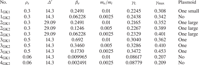
An extensive numerical simulation campaign, reported in tables 1 and 2, was carried out to study the physical conditions under which plasmoids appear.
Gyrofluid and fluid simulations.

Gyrokinetic simulations.

Each simulation is identified by a code of the form $p_{F/{\rm GF}/{\rm GK} \, r}$ , where $p$
 and $r$
 are integers and $F$
 , GF and GK indicate whether the simulation is carried out in the fluid limit, with the gyrofluid model or with gyrokinetic model, respectively. For all the simulations, the value of the electron skin depth is fixed to $d_e=0.085$
 . Simulations with the same number $p$
 are characterised by the same values of $d_e$
 , $\rho _s$
 and $\varDelta '$
 . For a fixed $p$
 , different values of the index $r$
 , on the other hand, indicate different values of $\beta _e$
 (and, consequently, of $m_e/m_i$
 ), with $\beta _e$
 decreasing as $r$
 increases. Not all the simulations of table 1 have a corresponding simulation in table 2 and vice versa, although this is the case for most of the simulations. In particular, we point out that, because gyrokinetic simulations always have a finite value of $\beta _e$
 , strictly speaking there is no gyrokinetic counterpart for the fluid simulations, which formally correspond to the $\beta _e \rightarrow 0$
 limit.
For all the gyrokinetic simulations, the temperature ratio is set to $\tau = 10^{-3}$ , where the ion Larmor radius is $\sqrt {\tau }\rho _s$
 . As mentioned before, the gyrofluid model assumes $\tau \rightarrow 0$
 . Therefore, in both the gyrofluid and gyrokinetic approach, the ion Larmor radius effects are neglected.
For $p=1,3,4$ , the initial current sheet extends along $-{\rm \pi} < y < {\rm \pi}$
 , which gives $\varDelta '_{m=1}=14.3$
 for the initially excited mode, and $\varDelta '_{m=2}=1.23$
 for the generated mode $m=2$
 . For $p=2$
 , we enlarge the box along $y$
 to $-1.4{\rm \pi} < y < 1.4{\rm \pi}$
 , which gives $\varDelta '_{m=1}=29.09$
 , and the modes $m=2$
 and $m=3$
 are generated with $\varDelta _{m=2}'=5.94$
 and $\varDelta _{m=3}'=0.46$
 .
As a first general comment, we observe, by comparing gyrofluid and gyrokinetic simulations with the same indices $p$ and $r$
 , that, in terms just of appearance or absence of plasmoids, gyrofluid simulations agree with the gyrokinetic ones. Therefore, in this respect, we can conclude that the quasi-static closure for the electrons and the suppression of ion gyrocentre fluctuations, do not affect critically the stability of the nonlinear current sheet. However, as discussed in the following sections, differences appear in terms of the number and size of plasmoids. In particular, when more than one plasmoid is observed, this is indicated in tables 1 and 2, generically, as ‘several plasmoids’. The number of plasmoids in the same simulation can indeed vary in time, as plasmoids can form at different times and pairs of plasmoids can merge into a single one.
3.1. Growth rates
Before discussing in detail the plasmoid instability, we briefly comment about the linear growth rate of the $m=1$ tearing mode excited by the perturbation of the initial equilibria (2.41a–c). In the tables, we reported the value of the linear and maximum growth rate of the tearing instability, evaluated measuring the following quantity at the $X$
 -point

The linear growth rate obtained by the two approaches are in very good agreement.
For a fixed $p$ , increasing $\beta _e$
 and $m_e/m_i$
 stabilises the tearing mode. This aligns with the results of Numata et al. (Reference Numata, Dorland, Howes, Loureiro, Rogers and Tatsuno2011), in which similar stabilisation effects are observed when increasing $\beta _e$
 and the mass ratio.
Figure 1 shows the solution of the dispersion relation derived from the fluid model by Porcelli (Reference Porcelli1991) given by

As shown in figure 1, for $d_e=0.085$ and $\rho _s=0.3$
 , this dispersion relation agrees with the linear growth rate of $1_F$
 and $2_F$
 . With Ohm's law (2.21) that retains first-order FLR corrections as well as corrections due to parallel magnetic perturbations, we can extend the dispersion relation (3.2) by replacing $d_e$
 and $\rho _s$
 with the effective parameters $d_e'=\sqrt {1 -\beta _e/4} d_e$
 and $\rho _s'=\sqrt {2/(2 +\beta _e)} \rho _s$
 , respectively. The solution of this small FLR dispersion relation, for $\beta _e=0.12$
 and $\beta _e=0.24$
 , are shown on figure 1 and allow a good prediction of the linear growth rate of the gyrofluid simulations for $\rho _s=0.3$
 . In particular, this permits the isolation of the stabilising effect of $\beta _e$
 on the growth rate, when only $\beta _e$
 is varied. Such stabilising effect becomes easier to identify in the small $\varDelta '$
 limit, in which (3.2) (with $d_e$
 and $\rho _s$
 replaced by the corresponding primed effective parameters) yields $\gamma \, \propto \, d_e' \rho _s'\varDelta ' \sim d_e \rho _s (1 - (3/8)\beta _e)\varDelta '$
 for $\beta _e \rightarrow 0$
 .
By comparing the growth rate results, for a fixed mass ratio, of simulations $p=1, 3, 4$ , we note that increasing $\beta _e$
 and $\rho _s$
 , as $\rho _s \sim \sqrt {\beta _e/2}$
 , destabilises the tearing mode. Increasing these parameters can be seen as fixing the background density, the ion mass and the guide field amplitude, while increasing the electron temperature. It was shown numerically in Numata & Loureiro (Reference Numata and Loureiro2015) and Granier et al. (Reference Granier, Borgogno, Grasso and Tassi2022b) that, in this latter situation, the linear tearing growth rate is first ruled by the destabilising effect of the sonic Larmor radius. However, in cases where the electron temperature is high enough for the effects of $\rho _e$
 to take over those of $\rho _s$
 , the linear growth rate is damped. Here, we find ourselves in the first case, for which the effects of the sonic Larmor radius are visibly dominant.
In the nonlinear phase, a slight discrepancy in the maximum growth rate can be noted for the largest $\beta _e$ values. Figure 2 shows the value of $\gamma _{\rm max}$
 for the set of simulations $p=2$
 and $p=3$
 . The gyrofluid and gyrokinetic simulations yield the same dependence of $\gamma _{\rm max}$
 on the parameters, with the gyrofluid simulations slightly underestimating the maximum growth rate measured in the nonlinear phase. This discrepancy suggests that, for large values of $\beta _e$
 and during the nonlinear phase, the efficiency of the gyrofluid model to reproduce the gyrokinetic results becomes limited. As commented in § 2.3, one reason for this might be the absence of ion gyrocentre density and parallel velocity fluctuations, which occurs in the gyrofluid model, even for large $\beta _e$
 , due to the imposed condition (2.39a,b).
Maximum growth rates of the collisionless tearing mode as a function of $\beta _e$ , for the cases (a) $p=2$
 and (b) $p=3$
 .

3.2. Remarks on the numerical resolution
It is important to anticipate the role of the resolution in this study. In the forming nonlinear current sheet, tearing modes grow and can become unstable at different times. The current sheet can therefore be broken by multiple dominant modes, and the number of plasmoids is highly sensitive to the resolution used. Given that the fluid simulations $2_F$ and $3_F$
 were those which allowed the formation of several plasmoids, we carried out resolution tests with the gyrofluid code on these two simulations to determine the necessary number of points along $y$
 , that does not prevent the growth of large mode numbers.
Table 3 reports the number of visible plasmoids for simulation $2_F$ as a function of the number of points and indicates their order of appearance. The convergence is reached for a resolution of $2304^2$
 .
number of visible plasmoids for simulation $2_F$ for different grids.

For $3_F$ , which is close to marginal stability, a spatial discretisation smaller than $2 L_y / n_y \sim 0.0078$
 was needed. Unfortunately, it is not foreseeable to perform gyrokinetic simulations with such a high resolution. Therefore, a grid of $256 \times 128$
 points has been used for all the gyrokinetic runs. We compared these gyrokinetic simulations to fluid/gyrofluid simulations performed with a nearly identical resolution. However, since the fluid code is much less demanding in computation time, we also performed the fluid simulations with grids up to $2304^2$
 points.
3.3. Effect of $\beta _e$ on the plasmoid onset

In this section we present how the $\beta _e$ parameter changes modify the critical aspect ratio for the plasmoid formation. We measure the current sheet aspect ratio using the current density $j_{\parallel }$
 . The length is defined such that the current distribution from the $X$
 -point to $L_{{\rm cs}}/2$
 equals a specific value $\alpha$


where ${\rm \Delta} y$ is the mesh length along $y$
 and $N$
 indicates the number of points from $y=0$
 to $y=L_{{\rm cs}}/2$
 . The constant $\alpha$
 is taken to $1/3$
 as it gives good measurement of the length of the region with a strong current. Formula (3.3) allows us to apply a single consistent method for all the simulations, while taking into account the reduction of the current intensity along the layer. The width of the current sheet corresponds to the distance between the two points along $x$
 where the value of $j_{\parallel }$
 takes the same value as at the point $(0,L_{{\rm cs}}/2)$
 .
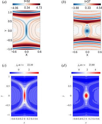
We focus first on the comparison of the series of simulations for $p=1$ , starting with the higher $\beta _e$
 case, for which $\beta _e=0.2491$
 . The contour plots of the parallel electron velocity $u_e$
 (proportional to the parallel current density), for the gyrofluid simulation $1_{\rm GF1}$
 and of the current density, $j_{\parallel }$
 , for the gyrokinetic simulations $1_{\rm GK1}$
 , are shown in figure 3. Isolines of the magnetic potential, showing the topology of the magnetic field, are overplotted. Both approaches indicate the formation of an island at the $X$
 -point. For the fluid simulation, the aspect ratio is $A_{{{\rm cs}_f}}=4.90$
 . In the gyrokinetic case, we measure $A_{{{\rm cs}_k}}=4.03$
 . We observe a persistent difference between the value of the gyrofluid and gyrokinetic aspect ratios, which is explained by the difference in resolution. However, their evolution according to the parameters are in agreement.
(a,b) Contour of the parallel electron velocity $u_e$ (proportional to the parallel current density and normalised by $\widehat {d_i}/L$
 and by the Alfvén velocity $v_A$
 ) for simulation $1_{\rm GF1}$
 . (c,d) Contour of the parallel current density $j_{\parallel }$
 (normalised by $e n_0 v_A$
 ) of simulation $1_{\rm GK1}$
 . The difference in normalisation conventions leads to a factor $-d_i = -0.85$
 between the two quantities. Isolines of the magnetic potential are superimposed on all the contours.

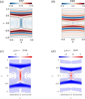
For the lowest $\beta _e$ cases, for which $\beta _e=0.06228$
 , the contour plots of the simulations $1_{\rm GF2}$
 and $1_{\rm GK2}$
 , are shown in figure 4. The two simulations lead to the formation of a stable current sheet having an aspect ratio decreasing in time. The maximum aspect ratio is reached when the growth rate measure by (3.3) has reached its maximum value and the process enters the saturation phase. From the gyrofluid simulation we measured a maximum aspect ratio $A_{{{\rm cs}_f}}=5.11$
 . In the gyrokinetic case, the aspect ratio is $A_{{{\rm cs}_k}}=4.14$
 . The measured aspect ratio are very close to those obtained for $\beta _e=0.2491$
 , and yet, no island develops at the $X$
 -point.
(a,b) Contour of the electron velocity $u_e$ (proportional to the parallel current density) for simulation $1_{\rm GF2}$
 . (c,d) Contour of the parallel current density $j_{\parallel }$
 of simulation $1_{\rm GK2}$
 . The difference in normalisation conventions leads to a factor $-d_i = -1.7$
 between the two quantities. Isolines of the magnetic potential are superimposed on all the contours.

Exciting only the mode $m=1$ results in the development of secondary modes due to nonlinear interactions. The growth of these modes can be observed by comparing their amplitude evolution over time. As is typical for tearing instability, we observe that these modes grow faster than the mode $m=1$
 , but their amplitudes remain smaller in our simulations. In addition, we find that increasing $\beta _e$
 (while increasing the mass ratio) slows down the growth of these generated modes in all simulations. In simulation set $p=1$
 , there is the mode $m=2$
 , which according to theory has a positive $\varDelta '$
 . However, in the case with $\beta _e=0.2491$
 , for which mode 2 grows more slowly, a plasmoid forms at the $X$
 -point. It is worth pointing at the reference Del Sarto & Deriaz (Reference Del Sarto and Deriaz2017) in which they observed that after the saturation of $m=1$
 , the linear growth of $m=2$
 persists and dominates until the formation of a second island, despite the absence of a secondary evolving current sheet. However, here, by examining the evolution of the amplitude of the Fourier modes for which $\varDelta ' > 0$
 , as well as the time derivative of their amplitude evolution, we see that the appearance of plasmoids occurs after the saturation of all the subdominant primary modes that fulfill the instability criterion for the initial magnetic equilibrium.
For $1_{\rm GF1}$ , we measured $L_{{\rm cs}}/\rho _s \sim 2$
 and $L_{{\rm cs}}/\rho _e \sim 12$
 , and the plasmoid formation indicates that the critical aspect ratio is $A_\star < L_{{\rm cs}}/\delta _{{\rm cs}} \sim 4$
 . In contrast, for $1_{\rm GF2}$
 , we have $L_{{\rm cs}}/\rho _s \sim 3$
 and $L_{{\rm cs}}/\rho _e \sim 64$
 , and the critical aspect ratio has not been reached, $A_\star > L_{{\rm cs}}/\delta _{{\rm cs}} \sim 4$
 , indicating that no plasmoids are formed. In this first set of tests, we are operating at the boundary between stability and instability. By increasing $\beta _e$
 , electron FLR effects become especially significant in the inner region, providing an additional mechanism to break the frozen-in condition. These combined effects are crucial in reducing the critical aspect ratio of the secondary current sheet. In addition to the electron FLR effects, a notable difference between the regimes of negligible $\beta _e$
 and finite $\beta _e$
 is the behavior of the perpendicular velocity flow. In the fluid case, the perpendicular velocity is determined by $\boldsymbol {u}_{\perp }= \hat {z} \times \boldsymbol {\nabla } \phi$
 , whereas in the gyrofluid case, a nonlinear grad-B drift due to the non-uniformity of the parallel magnetic field also affects the perpendicular velocity, which is given by $\boldsymbol {u}_{\perp }= \hat {z}\times \boldsymbol {\nabla } (G_{10e} \phi - \rho _s^2 2 G_{20e} B_\parallel )$
 . When examining the velocity vector field in the $x$
 direction near the reconnection points, we observe that it is not uniform in time, we see intermittent acceleration and deceleration, resulting in a non-uniform flow. This non-uniformity of the inflows and outflows becomes more pronounced as the grad-B drift becomes significant.
In the series of simulations for $p=2$ , the idea is to consider the same parameters as those for $p=1$
 but with a longer forming current sheet. Since highly unstable primary reconnecting modes favour the formation of extended secondary current sheets we consider a larger domain size along the $y$
 direction, with $L_y=1.4 {\rm \pi}$
 , that corresponds to $\varDelta '=29.9$
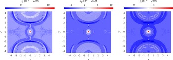
 . The other parameters are kept the same. In this case, the current sheet has an aspect ratio above the critical value, indicating that plasmoid formation occurs also for $\beta _e=0$
 . Figure 5 shows the plasmoids obtained at the end of the simulations $2_{\rm GK1}$
 –$2_{\rm GK3}$
 . The magnetic potential contour is shown as the plasmoid reaches its maximum size, which occurs in the saturation phase of the tearing instability. Figure 6 shows the evolution in time of the aspect ratio of the secondary current sheet. It can be seen that increasing $\beta _e$
 results in larger sized plasmoids, although, from the aspect ratio measurement, increasing $\beta _e$
 reduces the aspect ratio obtained just before the plasmoid onset.
Contour of the parallel current density $j_{\parallel }$ for simulations $2_{\rm GK3}$
 , $2_{\rm GK2}$
 and $2_{\rm GK1}$
 . Isolines of the magnetic potential are superimposed on all the contours.

Aspect ratio of the forming current sheet as a function of time for simulations $2_{\rm GK1}$ , $2_{\rm GK2}$
 and $2_{{\rm GK3}}$
 .

In comparison, figure 7 shows the aspect ratio obtained for the simulations $4_{\rm GK1}$ and $4_{\rm GK2}$
 . For this set of simulations, the effects of $\beta _e$
 are negligible and the parameters $\rho _s$
 and $\varDelta '$
 are smaller than those of simulations $2_{\rm GK1}$
 –$2_{\rm GK3}$
 . Nevertheless, despite a very different set of parameters, the two set of simulations lead to the formation of current sheets whose aspect ratio is almost identical. Yet, unlike cases $2$
 , cases $4$
 remain stable.
Aspect ratio of the forming current sheet as a function of time for the simulations $4_{\rm GK1}$ and $4_{\rm GK2}$
 .

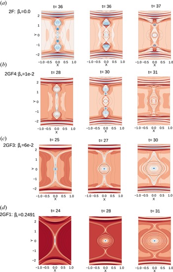
Figure 8 shows the evolution of the instability in detail for the runs $2_{F}$ , $2_{\rm GF4}$
 , $2_{\rm GF3}$
 and $2_{\rm GF1}$
 with the highest resolution. In the secondary current sheet, we observe that some modes may reach a high amplitude from an early stage and continue growing, while others may remain stable for a long time until they become unstable at a later stage and experience explosive growth. In the case $\beta _e = 0$
 , it was observed in Granier et al. (Reference Granier, Borgogno, Comisso, Grasso, Tassi and Numata2022a) that for $\rho _s \gg d_e$
 , the first plasmoids that break up the current sheet are symmetrically located above and below the $X$
 -point of the mode $m=1$
 . These plasmoids are then ejected from the current sheet, carried by the outflow, and merge with the island of the $m=1$
 tearing mode. A recent result obtained in a 2D collisionless fluid model (Grasso & Borgogno Reference Grasso and Borgogno2022) has indeed shown that $\rho _s$
 significantly enlarge the spectrum of the linear unstable reconnecting modes that develop in the presence of a sheared flow and magnetic field. Given the shape of the initial perturbation of the equilibrium, these plasmoids cannot coincide with the $O$
 -points of low tearing modes. For example, some of the $O$
 -points of modes 3, 4, 5 and 6 would grow at $1.4{\rm \pi} /3$
 , $2\times 1.4{\rm \pi} /4$
 , $1.4{\rm \pi} /5$
 and $2\times 1.4{\rm \pi} /6$
 , respectively. Instead, the position of the appearing $O$
 - and $X$
 -points of these new reconnection events indicates that the wavelength which has reached its nonlinear phase is associated with a large mode.
Contour of $u_e$ with isolines of $A_{\parallel }$
 . From (a) to (d) panels: $2_{F}$
 ($2304^2$
 ), $2_{\rm GF4}$
 , $2_{\rm GF3}$
 and $2_{\rm GF1}$
 ($2304\times 2400$
 ).

When $\beta _e$ is increased, we observe fewer plasmoids, as shown in figure 8. The emergence of these structures from the current starts when the associated mode reaches a sufficiently large amplitude. After they emerge, their growth becomes extremely rapid, taking only a few Alfvèn timescales to form. While increasing $\beta _e$
 may suggest a decrease in the critical aspect ratio, our observations reveal that it actually results in a slower growth rate of the modes propagating in the current sheet. Therefore, this parameter is also responsible for the slower development of these plasmoids, resulting in only one island reaching an explosive growth before the others. This island is located at the centre of the secondary current sheet and is therefore not affected by the upstream and downstream outflow, and ejects any other growing magnetic islands towards the $m=1$
 mode islands.
3.4. Validation of the plasmoid regime for $\rho _s \gg d_e$

A theory and numerical study developed by Granier et al. (Reference Granier, Borgogno, Comisso, Grasso, Tassi and Numata2022a) stated that, for a current sheet close to marginal stability, the regime $\rho _s \gg d_e$ promotes the plasmoid formation. In this reference, the simulations were carried out with the fluid model (2.16) and (2.17) which assumes a negligible mass ratio and a negligible $\beta _e$
 . In this subsection, we present a gyrokinetic validation of these results. In addition to observing a possible role played by the closure, we also compare the fluid results with those including a finite mass ratio of $m_e/m_i=0.005$
 , and consequently a small $\beta _e$
 . Moreover, as already recalled, the evolution of ion quantities such as $N_i$
 and $U_i$
 , prevented by the gyrofluid model, but present in the gyrokinetic simulations, might in principle also play a role.
Therefore, in this subsection we focus on the low $\beta _e$ regime and compare the simulation set for $p=3$
 , for which $\rho _s \gg d_e$
 , with the simulation set for $p=4$
 , for which $\rho _s \ll d_e$
 . These two sets of simulation lead to the formation of a secondary current layer close to the instability threshold. In the gyrofluid and fluid model, $\rho _s$
 is related to electron parallel compressibility effects and can be shown to be due to a non-isotropic component of the electron pressure tensor. When $\rho _s$
 becomes non-negligible, ion-sound Larmor effects become important, and the diamagnetic drift $\boldsymbol {z}\times \nabla _\perp ^2\rho _s^2 N_e$
 affects the perpendicular flow. This alters the structure of the current sheet and transforms it into a cross-shaped pattern aligned with the magnetic island separatrices, as described in Cafaro et al. (Reference Cafaro, Grasso, Pegoraro, Porcelli and Saluzzi1998). This effect is known to enhance the linear growth rate of the tearing mode significantly.
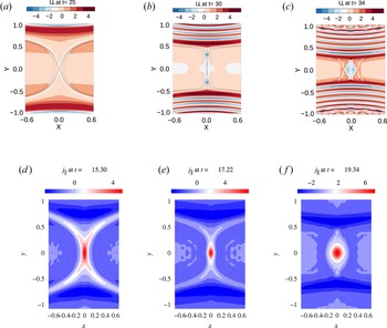
Figure 9 shows the evolution of the instability for the simulations $3_{\rm GK3}$ (lowest $\beta _e$
 gyrokinetic case of this series) and $3_F$
 . For the two approaches, the current sheet becomes plasmoid unstable. Also in this case the resolution plays an important role. With a resolution of $1728^2$
 , three plasmoids were visible in the simulations $3_F$
 . However, the same fluid simulation performed with a resolution $500\times 360$
 shows only one plasmoid. Since a resolution higher than that was not foreseeable with the gyrokinetic code, we used a grid of $256\times 128$
 points that allowed to observe one single plasmoid at the centre. In the regime $\rho _s \gg d_e$
 , the current aligns with the magnetic field lines, thus forming a cross shaped current sheet. This behavior is retrieved by the gyrokinetic simulation.
(a–c) Contour of the parallel current density $u_e=U_e$ for simulation $3_{F}$
 ($1728^2$
 ). (d–f) Contour of the parallel current density $j_{\parallel }$
 of simulation $3_{\rm GK3}$
 . The difference in normalisation conventions leads to a factor $-d_i = -1.7$
 between the two quantities. Isolines of the magnetic potential are superimposed on all the colour maps.

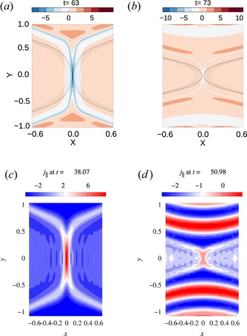
Figure 10 shows the evolution of the secondary current sheet for the cases $4_{\rm GK3}$ (lowest $\beta _e$
 gyrokinetic case of this series) and $4_F$
 . The current sheet formed in the two frameworks does not follow the separatrices but remains mainly aligned along $x=0$
 . For $4_F$
 , where ion-sound Larmor radius effects are negligible, the secondary current sheet has the dimensions $A_\star > A_{{\rm cs}} \sim 9$
 . This is consistent with the numerical results of Granier et al. (Reference Granier, Borgogno, Comisso, Grasso, Tassi and Numata2022a), which indicate that in this regime, an aspect ratio threshold of $A_{\star }^{(1)} \sim 10$
 is required for plasmoid growth. On the other hand, for $3_F$
 where $\rho _s > \delta _{{\rm in}}$
 , the threshold $A_\star ^{(2)}$
 decreases proportionally to $L_{{\rm cs}}/\rho _s$
 , and plasmoids form.
(a,b) Contour of the parallel current density $u_e=U_e$ for simulation $4_{F}$
 ($1728^2$
 ). (c,d) Contour of the parallel current density $j_{\parallel }$
 of simulation $4_{\rm GK2}$
 . The difference in normalisation conventions leads to a factor $-d_i = -1.7$
 between the two quantities. Isolines of the magnetic potential are superimposed on all the colour maps.

This comparison makes it possible to show that, if $L_{{\rm cs}}/d_e$ is sufficiently large, the current sheet becomes unstable regardless of the value of $\rho _s$
 . However, the effect of a large sonic Larmor radius is significant, when the system is marginally stable, to switch from a stable secondary current sheet to an unstable one. This is consistent with the fact that ion-sound Larmor radius effects allows for faster than exponential growth in the nonlinear phase (Aydemir Reference Aydemir1992).
4. Energy partition: similarities and differences between gyrokinetics and gyrofluid
4.1. Energy components
As we consider here a plasma with no collisions, the gyrokinetic system solved by AstroGK conserves the total energy (Hamiltonian) (Howes et al. Reference Howes, Cowley, Dorland, Hammett, Quataert and Schekochihin2006; Schekochihin et al. Reference Schekochihin, Cowley, Dorland, Hammett, Howes, Quataert and Tatsuno2009), normalised by $B_{0}^2/(4{\rm \pi} )$

where $\delta {\mathcal {F}}_{s}=g_{s} + (1/di) (2Z_{s}/(\tau _s \beta _e)) (\mathcal {J}_{0s}^2-1) \phi + d_i v_\perp ^2 \mathcal {J}_{1s}\mathcal {J}_{0s} B_\parallel$ is the perturbation of the particle distribution function for the species $s$
 . The first term is the perturbed entropy of the species $s$
 , while the second term and third terms are the energy of the perpendicular and parallel perturbed magnetic field. We can extract the first two moments from the perturbed particle distribution function as

where the perturbed density and parallel velocity of the particle of species $s$ are denoted as $n_s$
 and $u_s$
 , respectively, and $h_s'$
 contains all higher moments of the perturbed distribution function. By definition,

We can therefore decompose the expression (4.1) in the following way

The first term is the energy generated by the electron density variance, the second term is the kinetic energy of the parallel electron flow, and the third term is the free electron energy.
With regard to the collisionless gyrofluid model, the system of (2.1)–(2.5) possesses a conserved Hamiltonian given by

We remark that, as is shown in the Appendix, the form of the Hamiltonian (4.5), obtained from the quasi-static closure, is the same that one obtains by imposing what we refer to as an isothermal gyrofluid closure (the relations between $\phi, A_{\parallel }, B_\parallel$ and $N_e, U_e$
 will, however, be different in the two cases).
Using the relation (2.13) and (2.14) we can also write the Hamiltonian in terms of particle variables as follows:

When we consider the limit $\beta _e$ , $m_e/m_i \rightarrow 0$
 the Hamiltonian of the gyrofluid equations is reduced to

which is namely the Hamiltonian of the fluid (2.16) and (2.17). In (4.7), the contribution from left to right are the energy generated by the electron density fluctuation, the parallel electron kinetic energy, the perpendicular magnetic energy and the perpendicular plasma kinetic energy which is essentially the $\boldsymbol {E} \times \boldsymbol {B}$ flow energy.
4.2. Negligible $\beta _e$: fluid versus gyrokinetic

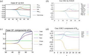
On figure 11 we present the comparison between the energy variation of the fluid case $1_F$ and that of the low $\beta _e$
 gyrokinetic case $1_{\rm GK3}$
 ($\beta _e=0.062$
 ). The variations are defined as $(1/2)\int \text {d} \boldsymbol {r}( \xi (x,y,t) - \xi (x,y,0)) / E(0)$
 where the function $\xi$
 can be replaced by the different contributions to $\hat {W}$
 and $H$
 (where $\hat {W}$
 is also considered in the 2D limit) and $E(0)$
 is the initial total energy. On the gyrokinetic plots, the four main energy channels are shown as solid lines. The solid purple line is the total ion energy variation. We also show the evolution of the variations relative to the density variance (dashed dotted), the parallel kinetic energy (densely dashed) and the perpendicular kinetic energy (loosely dashed), that are components of the total particle energy. The same channels are shown for the electrons in green.
Time evolution of the energy variations for the cases $1_F$ (a) and $1_{\rm GK3}$
 (b). (c) and (d) show the time evolution of the different contributions to the parallel kinetic energy for the corresponding simulations. No plasmoids in this case.

The amount of magnetic energy that is converted is identical between fluid and gyrokinetics and appears to be transferred mainly to the electrons. On the other hand, it is not identically distributed in the gyrokinetic and fluid frameworks. For the fluid simulations, the magnetic energy has no choice but to be converted into electron density fluctuations or electron parallel acceleration, whereas in the gyrokinetic case, there is little energy sent to these channels. This suggests that, in the gyrokinetic framework, the energy of the electrons increases due the fluctuations of the higher-order moments of the distribution function due to phase mixing (Loureiro, Schekochihin & Zocco Reference Loureiro, Schekochihin and Zocco2013; Numata & Loureiro Reference Numata and Loureiro2015), such as, for instance, the perpendicular and parallel electron temperature. It is likely that the magnetic energy is actually converted into thermal electron energy. Such possibility is prevented in the fluid case because, as a consequence of the closure, for $\beta _e \rightarrow 0$ , no temperature fluctuations are allowed.
The striking difference between the two approaches is that the parallel electron kinetic energy increases in the fluid case, whereas it is quasi-constant or decreasing in the gyrokinetic one (figure 11). In order to investigate the origin of this difference, we performed an initial condition check and decomposed the parallel electron kinetic energy. The decomposition leads to three energy components, namely the equilibrium part ($u_{\rm eq}^2$ ), the perturbation part ($\tilde {u}_e^2$
 ) and the cross term ($2\tilde {u}_eu_{\rm eq}$
 ). The change of each component is shown on the bottom panel of figure 11. The equilibrium contribution clearly does not change in time. The quadratic perturbation part is always positive but globally the variation of parallel electron kinetic energy can decrease because of the cross term becoming negative, which is the case for the gyrokinetic simulation. For the fluid case, the perturbation term increases considerably, leading to a positive variation of the parallel kinetic energy, since the electrons are highly accelerated for conservation of the total energy.
With regard to the ions, the closure assumptions imply an even rougher approximation of the ion dynamics, in the fluid case, with respect to gyrokinetics. In the gyrokinetic case, for low $\beta _e$ , we can see on figure 11 that the main component of the total ion energy consists of the perpendicular kinetic energy, which is included in the ${h_s}'$
 part in (4.4),Footnote 4 given by

where the perpendicular ion velocity $\boldsymbol {u}_{\perp, i}$ is calculated directly from its definition as a moment in the following way:

Note that the perpendicular flow holds the identity from the definition

where the perpendicular pressure tensor is given by

The perpendicular flow is given by the sum of $\boldsymbol {E}\times \boldsymbol {B}$ drift and diamagnetic drift of perturbed pressure.
In spite of the closure, the evolution of the energy component (4.8) is very similar to that of the $\boldsymbol {E}\times \boldsymbol {B}$ flow energy of the gyrofluid case. For a very small $\beta _e$
 , no parallel ion kinetic energy and parallel magnetic energy seems to be generated.
4.3. Finite $\beta _e$: gyrofluid versus gyrokinetic

When $\beta _e$ is very small, the FLR corrections become negligible and the particle and gyrocentre variables coincide. On the other hand, for non-negligible $\beta _e$
 , the electron Larmor radius becomes finite and the relations (2.11) and (2.12) allow us to relate the density and parallel velocity of the particles to those of the gyrocentres. In figure 12 we compare the gyrofluid energy variations with the gyrokinetic ones for $0 < \beta _e < 1$
 . For this purpose, we use the simulation set for $p=3$
 .
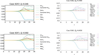
Time evolution of the energy variations for the cases $3_{GF}$ and $3_{GK}$
 .

In the plot referring to the gyrofluid energy, we show the variation of both the particles and gyrocentres energy. For instance, the curve referring to ‘Kin$_{\parallel e}$ ’ corresponds to the variation of $(1/2)\int {\rm d} x \, {\rm d} y d_e^2 u_e^2$
 , which is comparable to the second term of the gyrokinetic energy (4.4). The one referring to ‘Gyrocentre Kin$_{\parallel e}$
 ’ corresponds to the variation of $(1/2)\int {\rm d} x\, {\rm d} y d_e^2 U_e^2$
 . By increasing $\beta _e$
 , the difference between the variation of the energy of the gyrocentres and that of the particles increases. With finite $\beta _e$
 , we now note a loss of parallel kinetic energy of the electrons for the gyrofluid case, which is in better agreement with the gyrokinetic approach. Increasing $\beta _e$
 , will also generate more parallel magnetic energy, which is well reproduced by the gyrofluid model. On the other hand, the gyrokinetic cases indicate that a significant part of the magnetic energy is now converted into parallel ion kinetic energy. As mentioned previously, a limitation of the reduced gyrofluid model is that the ion parallel velocity has been ‘artificially’ removed by imposing $U_i=u_i=0$
 . The limitations of this assumption become evident, in particular, from figure 12 which shows that, in the gyrokinetic case, for sufficiently large $\beta _e$
 , the ion fluid is actually accelerated along the $\boldsymbol {z}$
 axis. On the other hand, it seems that despite this missing element, the gyrofluid model is suitable for studying the formation of plasmoid for $0<\beta _e<1$
 .
5. Conclusion
In this work, we have numerically investigated the plasmoid formation employing both gyrofluid and gyrokinetic simulations, assuming a finite, but small $\beta _e$ . We can conclude that the formation of plasmoids in a current sheet depends on various parameters, including the relative scales of the electron and ion-sound Larmor radii and the current sheet length. When electron FLR and ion-sound Larmor radius effects are taken into account, the critical aspect ratio $A_{{\rm cs}}^\star$
 for plasmoid formation is reduced, which promotes plasmoid growth. These results contribute to shedding light on collisionless reconnection mediated by the plasmoid instability and, in particular, on the role of the effects present at the electron scale.
This work has shown the ability of the reduced gyrofluid model to achieve relevant new insights into current-sheet stability and magnetic reconnection. In particular, predictions on marginal stability on current sheets, obtained by Granier et al. (Reference Granier, Borgogno, Comisso, Grasso, Tassi and Numata2022a) in the fluid limit, have been confirmed by gyrokinetic simulations. It also indicates that the fluid and gyrofluid models make it possible to obtain accurate results in short computational times.
The comparison between the gyrofluid and the gyrokinetic models has revealed key similarities and differences between the two frameworks, which gives insight into the important underlying physical effects. Indeed, the adopted gyrokinetic model is a $\delta f$ model from which the gyrofluid model can be derived with appropriate approximations and closure hypotheses. This has allowed us to directly identify possible limitations of the closures applied to the gyrofluid moments, that distinguish the gyrofluid model from its gyrokinetic parent model. We therefore presented the effect of the closure on the distribution and conversion of energy during reconnection. The closure, which does not allow for parallel temperature fluctuations, implies that gyrocentre moment fluctuations energies in which the magnetic energy can be converted, must be those of the electron density and parallel velocity. This is not in agreement with the gyrokinetic simulations, but does not seem to interfere with the formation of plasmoids. In particular, for relatively small but finite $\beta _e$
 , the hypothesis of absent parallel ion motion made in the gyrofluid framework is valid and does not affect the plasmoid instability. The gyrokinetic perpendicular ion velocity is well represented by the fluid $\boldsymbol {E}\times \boldsymbol {B}$
 velocity. On the other hand, gyrokinetic simulations show a large fraction of magnetic energy transferred to fluctuations of higher-order moments.
Acknowledgements
The authors thank the anonymous reviewers for valuable feedback.
Editor Alex Schekochihin thanks the referees for their advice in evaluating this article.
Declaration of interest
The authors report no conflict of interest.
Funding
The work of RN was partly supported by JSPS KAKENHI Grant Number 22K03568. The numerical simulations were performed using the EUROfusion high-performance computer Marconi Fusion and Galileo100 hosted at CINECA (project FUA35-FKMR and IsC86 MR-EFLRA), the computing facilities provided by the Mesocentre SIGAMME hosted by the Observatoire de la Côte d'Azur, as well as JFRS-1 supercomputer system at the Computational Simulation Centre of the International Fusion Energy Research Centre (IFERC-CSC) at the Rokkasho Fusion Institute of QST (Aomori, Japan) and on the ‘Plasma Simulator’ (NEC S$X$ -Aurora TSUBASA) of NIFS with the support and under the auspices of the NIFS Collaboration Research program (NIFS22KISS019). ET acknowledges support from the GNFM.
Appendix. Comparison between the gyrofluid isothermal and the quasi-static closure
In this appendix, we first show how the gyrofluid Hamiltonian (4.5) can be obtained from the gyrokinetic Hamiltonian (4.1) by applying the quasi-static closures and the assumptions described in § 2.3. Subsequently, we compare with the gyrofluid Hamiltonian obtained by applying what we refer to as gyrofluid isothermal closure.
The conserved energy (4.1) of the $\delta f$ gyrokinetic model used for the comparison in this paper can be expressed in terms of the gyrocentre perturbed distribution function

where $\langle \ \rangle _{\boldsymbol {X}_s}$ denotes the gyroaverage at constant guiding centre $\boldsymbol {X}_s$
 and $\boldsymbol {A}_\perp$
 is the magnetic vector potential associated with parallel magnetic perturbations, so that $\boldsymbol {\nabla } \times \boldsymbol {A}_{\perp } = B_\parallel \boldsymbol {z}$
 . In this way, we obtain

Note that, in (A2), we already took the spatial 2D limit, in order to directly obtain the gyrofluid Hamiltonian.
The gyrocentre perturbed distribution function can be developed as a series of its gyrocentre moments using Hermite and Laguerre polynomials. Here, we retain only the first two moments of the hierarchy for the two species, and apply two different closures, namely the quasi-static closure (Tassi et al. Reference Tassi, Passot and Sulem2020), and a gyrofluid isothermal closure, where the perpendicular and parallel gyrocentre temperature fluctuations $T_{\perp s } = T_{\parallel s}=0$ , are set equal to zero (as all the other higher-order gyrofluid moments). Such kind of closure is applied, for instance, by Scott (Reference Scott2010), although in this reference, gyrocentre temperature, as well as heat flux fluctuations, are retained and all the other higher-order moments are set equal to zero.
For the quasi-static closure, the expansion of the gyrocentre perturbed distribution functions for the two species are given by


The difference between electron and ion treatments in (A3) and (A4), is clearly due to the assumption (2.39a,b). We mention that, by retaining, in (A4), also ion gyrocentre density and parallel velocity fluctuations, and applying the same procedure described in the following, one can derive the energy of the 4-field Hamiltonian gyrofluid model described by Granier et al. (Reference Granier, Borgogno, Grasso and Tassi2022b).
In the case of the gyrofluid isothermal closure the truncated expansion simply gives


To simplify the infinite sums in (A3) and (A4), we can make use of the following relations (Szegö Reference Szegö1975)


where $L_n^{(1)}$ are associated Laguerre polynomials and of the expression of the operators (2.36) and (2.37a,b). We therefore obtain the following equality, that can be injected in (A3) and (A4),

We can now reduce the gyrokinetic Hamiltonian (A2) to gyrofluid ones by injecting the two sets of truncated perturbed gyrocentre distribution functions. In the quasi-static case, thanks to the relation (A9), all the contributions involving $G_{1n_s}$ and $G_{2n_s}$
 , with $n \geq 1$
 , cancel. It turns out that the two resulting gyrofluid Hamiltonians can be written in an identical form, which corresponds to the following

where we recall that $A_e=G_{10e} A_{\parallel } - d_e^2 U_e$ and the linear operators $\mathcal {L}_{U_e}$
 , $\mathcal {L}_\phi$
 and $\mathcal {L}_B$
 are given by


through the quasi-neutrality relation and the two components of Ampère's law. The expression (A10) coincides, up to integration by parts, to the Hamiltonian (4.5).
Evidently, the quasi-static quasi-neutrality equation and Ampère's law will differ from the isothermal ones. Therefore, the total conserved energy are actually evolving differently and the operators $\mathcal {L}_B$ , $\mathcal {L}_{\phi }$
 and $\mathcal {L}_{U_e}$
 are closure-dependent operators.
For instance, the explicit form of the quasi-neutrality relation, in the quasi-static case, can be written as

while in the case of the gyrofluid isothermal closure, we have

and where the $\varGamma _{0,1 e}$ operators are defined in Fourier space in the following way

where $I_n$ are the modified Bessel functions of order $n$
 .
A first comment is that the two closures, and consequently the two sets of static equations are, in fact, identical if we assume

which gives the approximations

On the other hand, the relations (A 17a,b) can be interpreted in a different way, i.e. considering the exact expressions (A 15a,b) for $\varGamma _{0e}$ and $\varGamma _{1e}$
 , and assuming that the expressions for $G_{10e}$
 and $G_{20e}$
 can be adapted to match the quasi-neutrality relations following from the two closures. In this way, from the first relation in (A 17a,b), one retrieves, for the case $s=e$
 , the approximate expression for the operators $G_{10s}$
 introduced by Dorland & Hammett (Reference Dorland and Hammett1993). The advantages of this approach have been more recently discussed also by Mandell, Dorland & Landreman (Reference Mandell, Dorland and Landreman2018). The above approach is indeed reminiscent of the approach used by Dorland & Hammett (Reference Dorland and Hammett1993) in order to find an expression for $G_{10s}$
 yielding a better agreement of liner gyrofluid theory with the linear gyrokinetic theory. A similar approach, accounting also for $G_{20s}$
 in a finite-$\beta$
 gyrofluid model, was followed by Despain (Reference Despain2011).
A second point is that, in the limit of negligible ion and electron Larmor radius, when considering $\tau _i \rightarrow 0$ and $\beta _e \rightarrow 0$
 , the two sets of static relations become identical and we obtain the same fluid Hamiltonian
For instance, both (A14) and (A13) will reduce to the quasi-neutrality relation

which is going to give rise to the $\boldsymbol {E}\times \boldsymbol {B}$ flow energy in the fluid Hamiltonian.