


1 Introduction
The goal of this paper is to confirm a conjectured criterion for zero-one dual characters of flagged Weyl modules due to Mészáros, St. Dizier, and Tanjaya [Reference Mészáros, Dizier and Tanjaya25, Conjecture 3.9]. A polynomial is called zero-one (or, multiplicity-free) if its coefficients are equal to either
 $0$
or
 $1$
. It is well known that dual flagged Weyl characters encompass Schubert and key polynomials as special cases. So our result leads to a unified proof for previously known criteria, respectively, for zero-one Schubert polynomials by Fink, Mészáros, and St. Dizier [Reference Fink, Mészáros and St Dizier10] and zero-one key polynomials by Hodges and Yong [Reference Hodges and Yong14].
Motivations of investigating zero-one dual characters of flagged Weyl modules are multifold. It was proved by Fink, Mészáros, and St. Dizier [Reference Fink, Mészáros and St9] that the supports of the dual character of a flagged Weyl module are exactly the same as the integer points in its Newton polytope. Hence, a zero-one dual flagged Weyl character is completely determined by the integer points in its Newton polytope.
As aforementioned, Schubert and key polynomials appear as special cases of dual characters of flagged Weyl models, see, for example, [Reference Fink, Mészáros and St9] and references therein. A criterion for zero-one Schubert polynomials was found by Fink, Mészáros, and St. Dizier [Reference Fink, Mészáros and St Dizier10], whose proof makes use of Magyar’s orthodontia formula for Schubert polynomials [Reference Magyar22, Reference Mészáros, Setiabrata and St Dizier23]. By the work of Knutson and Miller [Reference Knutson and Miller21], Schubert polynomials are the multidegree polynomials of matrix Schubert varieties. Particularly, zero-one Schubert polynomials correspond to multiplicity-free matrix Schubert varieties, and in this case, one could capture the entire information of K-polynomials (namely, Grothendieck polynomials) from that of zero-one Schubert polynomials [Reference Brion4–Reference Eur and Larson6, Reference Knutson20, Reference Mészáros, Setiabrata and St Dizier24, Reference Pechenik and Satriano27]. Moreover, for a permutation whose associated Schubert polynomial is zero-one, the CDG generators of the defining ideal of its matrix Schubert variety form a diagonal Gröbner basis [Reference Hamaker, Pechenik and Weigandt12, Reference Klein15].
A criterion (first announced in [Reference Hodges and Yong13, Theorem 4.10]) for zero-one key polynomials was proved by Hodges and Yong [Reference Hodges and Yong14] by employing two combinatorial models for key polynomials: the quasi-key model by Assaf and Searles [Reference Assaf and Searles3] and the Kohnert diagram model by Kohnert [Reference Kohnert17]. The algebraic motivation of studying zero-one key polynomials stems from the classification of Levi-spherical Schubert varieties [Reference Gao, Hodges and Yong11, Reference Hodges and Yong13].
Another notable subfamily of dual flagged Weyl characters are for northwest diagrams. This subfamily also includes Schubert and key polynomials as special cases. It was shown by Armon, Assaf, Bowling, and Ehrhard [Reference Armon, Assaf, Bowling and Ehrhard1] that the dual flagged Weyl character for a northwest diagram coincides with the Kohnert polynomial defined in [Reference Assaf and Searles2]. As remarked in [Reference Hodges and Yong14], the techniques they developed for zero-one key polynomials do not seem to extend to zero-one dual flagged Weyl characters for northwest diagrams.
We proceed by describing the criterion for zero-one dual characters of flagged Weyl modules, as stated in [Reference Mészáros, Dizier and Tanjaya25, Conjecture 3.9]. Let
 $[n]=\{1,2,\ldots , n\}$
. A subset D of boxes in the grid
 $[n]\times [n]$
is called a diagram. The flagged Weyl module
 $\mathcal {M}_{D}$
associated a diagram D is a module of the group B of invertible upper-triangular matrices over
 $\mathbb {C}$
[Reference Kraskiewicz and Pragacz18, Reference Kraśkiewicz and Pragacz19, Reference Magyar22], see Section 2 for the precise definition. The dual character of
 $\mathcal {M}_{D}$
, denoted
 $\chi _{D}(x)$
, is a polynomial in
 $x_1,\ldots , x_n$
, which coincides with the Schubert polynomial
 $\mathfrak {S}_w(x)$
when D is the Rothe diagram of a permutation w, and the key polynomial
 $\kappa _\alpha (x)$
when D is the skyline diagram of a composition
 $\alpha $
. The flagged Weyl modules have inspired considerable recent research interests, see, for example, [Reference Armon, Assaf, Bowling and Ehrhard1, Reference Fan and Guo7–Reference Fink, Mészáros and St Dizier10, Reference Mészáros, Setiabrata and St Dizier23, Reference Mészáros, Dizier and Tanjaya25, Reference Mészáros and Tanjaya26, Reference Peng, Lin and Sun28].
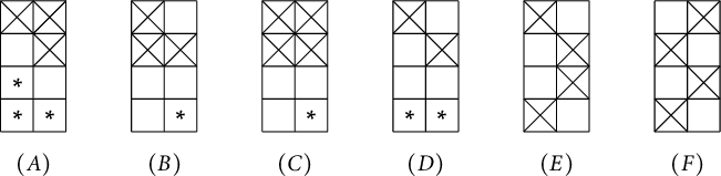
Following the terminology in [Reference Mészáros, Dizier and Tanjaya25], a multiplicitous configuration refers to one of the six instances of configurations listed in Figure 1. Here, a crossing “
 $\times $
” indicates the absence of a box, a blank square indicates the presence of a box, and a star “
 $*$
” indicates no restriction on the presence or absence of a box.
Multiplicitous configurations.

A diagram D is called multiplicitous if it contains one of multiplicitous configurations as a subdiagram, up to possibly swapping the order of the columns. This means that there exist row indices
 $i_1<i_2<i_3<i_4$
and column indices
 $j_1<j_2$
such that the subdiagram of D, which is restricted to rows
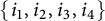 $\{i_1, i_2, i_3, i_4\}$
and columns
 $\{j_1, j_2\}$
, is either a multiplicitous configuration or a configuration obtained from a multiplicitous configuration by swapping its two columns. We call a diagram D multiplicity-free if it is not multiplicitous. So a multiplicity-free diagram avoids a total of 12 configurations.
In light of an observation in [Reference Fink, Mészáros and St Dizier10, Theorem 5.8], it is readily verified that if the dual character
 $\chi _{D}(x)$
is zero-one, then D must be multiplicity-free [Reference Mészáros, Dizier and Tanjaya25, Proposition 3.11]. This paper aims to prove the reverse direction which appears as [Reference Mészáros, Dizier and Tanjaya25, Conjecture 3.9].
Theorem 1.1 [Reference Mészáros, Dizier and Tanjaya25, Conjecture 3.9]
If D is a multiplicity-free diagram, then the dual character
 $\chi _{D}(x)$
is zero-one.
Combining Theorem 1.1 with the above mentioned [Reference Mészáros, Dizier and Tanjaya25, Proposition 3.11] gives a full criterion for zero-one dual Weyl characters.
Corollary 1.2 The dual character
 $\chi _{D}(x)$
is zero-one if and only if D is a multiplicity-free diagram.
The above corollary on the one hand specializes to the criterion for zero-one Schubert polynomials [Reference Fink, Mészáros and St Dizier10, Theorem 1] when D is the Rothe diagram of a permutation, and on the other hand to the criterion for zero-one key polynomials [Reference Hodges and Yong14, Theorem 1.1] when D is the skyline diagram of a composition.
This paper is structured as follows. In Section 2, we review the construction of the flagged Weyl module
 $\mathcal {M}_{D}$
, as well as some facts about its dual character
 $\chi _{D}(x)$
. Particularly, it will be seen that the coefficient of a monomial
 $x^a$
in
 $\chi _{D}(x)$
is equal to the dimension of the eigenspace in
 $\mathcal {M}_{D}$
corresponding to
 $x^a$
. Section 3 is devoted to several lemmas concerning the properties of multiplicity-free diagrams. In Section 4, we finish the proof of Theorem 1.1 which will be achieved by showing that when a diagram D is multiplicity-free, each eigenspace in
 $\mathcal {M}_{D}$
has dimension exactly equal to one. The arguments are combinatorial.
2 Dual characters of flagged Weyl modules
In this section, we give an overview of some basic information about flagged Weyl modules. We mainly follow the notation in [Reference Fink, Mészáros and St9, Reference Fink, Mészáros and St Dizier10].
For the square grid
 $[n]\times [n]$
, let us use
 $(i, j)$
to denote the box in row i and column j in the matrix coordinate. Recall that a diagram D is a subset of boxes in
 $[n]\times [n]$
. Write
 $D=(D_{1}, D_{2},\ldots , D_{n})$
, where, for
 $1\leq j\leq n$
,
 $D_j$
stands for the j-th column of D. We shall often represent
 $D_j$
by a subset of
 $[n]$
, that is,
 $i\in D_j$
if and only if the box
 $(i,j)$
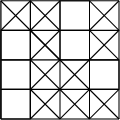
belongs to D. For example, the diagram in Figure 2 can be written as
 $D=(\{2,3,4\},\emptyset ,\{1,2\},\{3\})$
. As before, we use crossings to represent the absence of boxes.
A diagram in
 $[4]\times [4]$
.

For two k-element subsets
 $R=\{r_1< \cdots <r_k\}$
and
 $S= \{s_1< \cdots <s_k\} $
of
 $[n]$
, write
 $R\leq S$
if
 $r_i\leq s_i$
for
 $1\leq i\leq k$
. This defines a partial order, called the Gale order, on all k-element subsets of
 $[n]$
. For a given subset S of
 $[n]$
, the collection of subsets
 $R\leq S$
constitutes the basis of a matroid, called Schubert matroid, on the ground set
 $[n]$
[Reference Fink, Mészáros and St9]. It is worth mentioning that the Gale order plays an important role in the study of the positroid decomposition of (positive) Grassmannians [Reference Knutson, Lam and Speyer16, Reference Postnikov29]. For two diagrams
 $C=(C_{1}, \ldots , C_{n})$
and
 $D=(D_{1}, \ldots ,D_{n})$
, write
 $C\leq D$
if
 $C_{j}\leq D_{j}$
for each
 $1\leq j\leq n$
.
Let
 $\mathrm {GL}(n,\mathbb {C})$
be the general linear group of
 $n\times n$
invertible matrices over
 $\mathbb {C}$
, and B the Borel subgroup of
 $\mathrm {GL}(n,\mathbb {C})$
consisting of all upper-triangular matrices. Let Y be the upper-triangular matrix of variables
 $y_{ij}$
with
 $1\leq i\leq j\leq n$
:
 $$ \begin{align*} Y= \begin{bmatrix} y_{11} & y_{12} & \ldots & y_{1n}\\ 0 & y_{22} & \ldots & y_{2n}\\ \vdots & \vdots & \ddots & \vdots\\ 0 & 0 & \ldots & y_{nn} \end{bmatrix}. \end{align*} $$
Denote by
 $\mathbb {C} [Y]$
the linear space of polynomials over
 $\mathbb {C}$
in the variables
 $\{y_{ij}\}_{i\leq j}$
. Define the (right) action of B on
 $\mathbb {C} [Y]$
by
 $f(Y)\cdot b=f(b^{-1}\cdot Y)$
, where
 $b\in B$
and
 $f\in \mathbb {C} [Y]$
. For two subsets R and S of
 $[n]$
with the same cardinality, we use
 $Y^{R}_{S}$
to represent the submatrix of Y obtained by restricting to rows indexed by R and columns indexed by S. It is not hard to check that
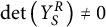 $\det \left (Y^{R}_{S}\right )\neq 0$
if and only if
 $R\leq S$
. Given two diagrams
 $C=(C_{1}, \ldots , C_{n})$
and
 $D=(D_{1}, \ldots , D_{n})$
with
 $C\leq D$
, denote
 $$\begin{align*}\mathrm{det}\left(Y_{D}^C\right)=\prod_{j=1}^{n}\mathrm{det}\left(Y_{D_{j}}^{C_{j}}\right). \end{align*}$$
The flagged Weyl module
 $\mathcal {M}_{D}$
for D is a subspace of
 $\mathbb {C} [Y]$
defined by
 $$ \begin{align*} \mathcal{M}_{D}=\mathrm{Span}_{\mathbb{C}}\left\{\mathrm{det}\left(Y_D^C\right)\colon C\leq D\right\}, \end{align*} $$
which is a B-module with the action inherited from the action of B on
 $\mathbb {C} [Y]$
.
Let X be the diagonal matrix with diagonal entries
 $x_{1},\ldots ,x_{n}$
. The character of
 $\mathcal {M}_{D}$
is defined by
 $$\begin{align*}\mathrm{char}(\mathcal{M}_{D})(x_{1},\ldots, x_{n})=\mathrm{tr}(X\colon \mathcal{M}_{D}\rightarrow \mathcal{M}_{D}).\end{align*}$$
It can be directly checked that
 $\mathrm {det}\left (Y_{D}^C\right )$
is an eigenvector of X with eigenvalue
 $$\begin{align*}\prod_{j=1}^n\prod_{i\in C_j}x_i^{-1}.\end{align*}$$
The dual character is defined as
 $$ \begin{align*} \chi_{D}(x):=\mathrm{char}(\mathcal{M}_{D})(x_{1}^{-1},\ldots,x_{n}^{-1}). \end{align*} $$
Hence, the coefficient of a monomial
 $x^a$
in
 $\chi _{D}(x)$
is equal to the dimension of the corresponding eigenspace:
 $$ \begin{align} [x^a]\,\chi_{D}(x)=\dim \mathrm{Span}_{\mathbb{C}}\left\{\mathrm{det}\left(Y_{D}^C\right)\colon C\leq D, \, x^C=x^a\right\}, \end{align} $$
where
 $$\begin{align*}x^{C}=\prod_{j=1}^{n}\prod_{i\in C_{j}} x_{i}. \end{align*}$$
In particular, the set of monomials appearing in
 $\chi _{D}(x)$
is
 $ \left \{x^C\colon C\le D\right \}$
.
Proposition 2.1 The dual character
 $\chi _{D}(x)$
is zero-one if and only if each eigensapce on the right-hand side of (1) has dimension one.
We end this section with a combinatorial expression for the generator
 $\mathrm {det}\left (Y_{D}^C\right )$
. A flagged filling of a diagram
 $D=(D_1,\ldots , D_n)$
is a filling of the boxes of D with positive integers such that
-
(1) each box receives exactly one integer, and the entries in each column are distinct;
-
(2) the entry in the box
 $(i,j)\in D$
cannot exceed i.

Let
 $F=(F_1,\ldots , F_n)$
be a flagged filling of D, where, for
 $1\leq j\leq n$
,
 $F_j$
denotes the j-th column of F. Define the inversion number
 $\mathrm {inv}(F)$
of F as follows. Let
 $w=w_1\cdots w_m$
be the word obtained by reading the entries of
 $F_j$
from top to bottom. Denote by
 $\mathrm {inv}(F_j)$
the inversion number of w, namely,
 $$\begin{align*}\mathrm{inv}(F_j)=\#\{(r, s)\colon 1\leq r<s\leq m, \ w_r>w_s\}. \end{align*}$$
In the case when
 $D_j$
is empty, we adopt the convention that
 $\mathrm {inv}(F_j)=0$
. Define
 $$\begin{align*}\mathrm{inv}(F)=\mathrm{inv}(F_1)+\cdots +\mathrm{inv}(F_n). \end{align*}$$
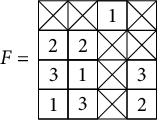
For the flagged filling depicted in Figure 3,
A flagged filling.

the column reading words are
 $231, 213, 1$
and
 $32$
from left to right, and so we have
 $\mathrm {inv}(F)=2+1+0+1=4$
. Assign a weight to F in the following way:
 $$ \begin{align*} y^{F}=\prod_{(i, j)\in D}y_{c_{ij}i}, \end{align*} $$
where
 $c_{ij}$
is the entry of F filled in the box
 $(i, j)$
. For example, the flagged filling in Figure 3 gives
 $$\begin{align*}y^{F}=y_{11}\,y_{22}^2\,y_{13}\,y_{33}^2\,y_{14}\,y_{24}\,y_{34}. \end{align*}$$
For
 $C\leq D$
, let
 $\mathcal {F}_{D}(C)$
denote the set of flagged fillings
 $F=(F_1,\ldots , F_n)$
of D such that for
 $1\leq j\leq n$
, the set of entries in
 $F_j$
is exactly
 $C_j$
. The following proposition appears as [Reference Peng, Lin and Sun28, Lemma 2.2].
Proposition 2.2 For
 $C\leq D$
, we have
 $$ \begin{align}\mathrm{det}\left(Y_{D}^C\right)=\sum_{F\in \mathcal{F}_{D}(C)}\mathrm{sgn}(F)\cdot y^{F}, \end{align} $$
where
 $\mathrm {sgn}(F)=(-1)^{\mathrm {inv}(F)}$
.
As explained in [Reference Peng, Lin and Sun28, Remark 2.3], the formula in (2) may not be cancellation-free, that is, there may exist distinct fillings in
 $\mathcal {F}_{D}(C)$
that contribute the same weight, but have opposite signs.
3 Multiplicity-free diagrams
In this section, we investigate the distribution of boxes in a multiplicity-free diagram. This will be a step stone in the proof that each eigenspace for a multiplicity-free diagram has dimension exactly equal to one.
Clearly, the dual character
 $\chi _{D}(x)$
is independent of the order of columns of D. We say that two diagrams are equivalent if one can be obtained from the other by reordering the columns. We shall designate a particular representative in the class of diagrams equivalent to D. Such a representative is called the normalization of D.
3.1 Normalization of diagrams
Let
 $D=(D_1,\ldots , D_n)$
be a diagram. The normalization, denoted
 $\mathrm {Norm}(D)$
, of D is the unique diagram equivalent to D by rearranging the columns in the following way. For
 $1\leq j\leq n$
, let
 $\overline {D}_j=([n]\setminus D_j)\cup \{\infty \}$
. For
 $ {D}_{j_1}\neq {D}_{j_2}$
, suppose that
 $$\begin{align*}\overline{D}_{j_1}=\{a_1<\cdots<a_s<a_{s+1}=\infty\},\ \ \ \ \ \overline{D}_{j_2}=\{b_1<\cdots<b_t<b_{t+1}=\infty\}. \end{align*}$$
Define
 $ {D}_{j_1}\prec {D}_{j_2}$
if
 $\overline {D}_{j_1}<_{\mathrm {lex}}\overline {D}_{j_2}$
in the lexicographic order, that is, there exists some index k such that
 $a_i=b_i$
for
 $1\leq i<k$
and
 $a_k<b_k$
. The usage of
 $\infty $
in
 $\overline {D}_{j}$
is to ensure that any two distinct columns of D are comparable. Now,
 $\mathrm {Norm}(D)$
is defined by rearranging the columns of D increasingly from left to right with respect to
 $\prec $
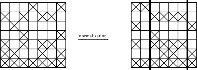
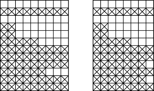
. See Figure 4 for an illustration of the normalization of a diagram.
An illustration of normalization.

A diagram D is called normalized if
 $D=\mathrm {Norm}(D)$
. Given a normalized diagram D, we partition the columns of D into distinct regions, according to the positions of the first crossing in each column. Here, the crossings in each column are counted from top to bottom. Precisely, columns of D belong to the same region if the first crossings in these columns lie in the same row. For example, the right normalized diagram in Figure 4 is partitioned into three regions, as divided by lines in boldface.
3.2 Columns in the same region
In this subsection, we analyze the distribution of boxes of a diagram
 $D=(D_1,\ldots , D_n)$
in the same region. We could always assume that each column in
 $[n]\times [n]$
has at least two “
 $\times $
” since otherwise one may embed D into a larger grid
 $[m]\times [m]$
with
 $m>n$
. With this in mind, we distinguish the columns of D into three types, according to the number of boxes below the second crossing. For
 $1\leq j\leq n$
, we say that
-
•
$D_j$
is of
$\mathrm {Type\ I} $
if there is no box of
$D_j$
below the second crossing; -
•
$D_j$
is of
$\mathrm {Type\ II} $
if there is exactly one box of
$D_j$
below the second crossing; -
•
$D_j$
is of
$\mathrm {Type\ III} $
if there are at least two boxes of
$D_j$
below the second crossing.


Define the signature of
 $D_j$
as the number of boxes of
 $D_j$
lying between the first and the second crossings. For example, the third column in the right diagram in Figure 4 is a Type II column with signature equal to 1. When D is a normalized diagram, the signatures of columns in the same region are weakly increasing from left to right.
Lemma 3.1 Let
 $D=(D_1,\ldots , D_n)$
be a normalized multiplicity-free diagram. Consider the columns of D in the same region. Suppose that a column
 $D_j$
does not reach the maximum signature among columns in the region. Then
 $D_j$
must be of
 $\mathrm {Type\ I} $
.
Proof Since
 $D_j$
does not reach the maximum signature, there exists a column
 $D_{j^{\prime }}$
with
 $j<j^{\prime }$
in the same region such that
 $D_{j^{\prime }}$
has a larger signature than
 $D_j$
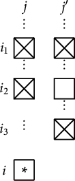
. Assume that the first two crossings in column j are at the positions
 $(i_1,j)$
and
 $(i_2,j)$
. Since
 $D_j$
and
 $D_j^{\prime }$
lie in the same region, the first crossing in column
 $j^{\prime }$
lies in row
 $i_1$
. Suppose that the second crossing in column
 $j^{\prime }$
lies in row
 $i_3$
. Then we have
 $i_3>i_2$
, and so the box
 $(i_2, j^{\prime })$
belongs to
 $D_j^{\prime }$
. See Figure 5 for an illustration.
An illustration for the proof of Lemma 3.1.

Let
 $(i,j)$
be any box below
 $(i_2, j)$
. We conclude that
 $(i,j)$
does not belong to
 $D_j$
since otherwise the subdiagram of D, which is restricted to rows
 $\{i_1, i_2, i\}$
and columns
 $\{j, j^{\prime }\}$
, would form the configuration obtained by swapping the columns of
 $(A)$
in Figure 1. This implies that
 $D_j$
is a column of Type I.
From Lemma 3.1, we see that if there are
 $\mathrm {Type\ II} $
or
 $\mathrm {Type\ III} $
columns occurring in the same region, then they must be columns with the maximum signature. We discuss this in detail in the next lemma.
Lemma 3.2 Let
 $D=(D_1,\ldots , D_n)$
be a normalized multiplicity-free diagram. Consider the columns in the same region. Then
-
(1)
$\mathrm {Type\ II} $
columns and
$\mathrm {Type\ III} $
columns cannot occur simultaneously. -
(2) If there is a
$\mathrm {Type\ II} $
column occurring, then all
$\mathrm {Type\ II} $
columns have the same configuration (In this case, the region starts with some
$\mathrm {Type\ I} $
columns, followed by some copies of a
$\mathrm {Type\ II} $
column, see the left picture in Figure 6 for an illustration).Figure 6:Illustrations of the regions in (2) and (3) of Lemma 3.2, respectively.
-
(3) If there is a
$\mathrm {Type\ III} $
column occurring, then this is the only
$\mathrm {Type\ III} $
column in the region (In this case, the region starts with some
$\mathrm {Type\ I} $
columns, followed by a single
$\mathrm {Type\ III} $
column, see the right picture in Figure 6 for an illustration).


Proof (1) Suppose to the contrary that there are both a
 $\mathrm {Type\ II} $
column (say,
 $D_{j_1}$
) and a
 $\mathrm {Type\ III} $
column (say,
 $D_{j_2}$
) occurring in the same region. We only consider the case for
 $j_1<j_2$
, and the arguments for
 $j_1>j_2$
are the same. Since column
 $j_1$
and column
 $j_2$
are in the same region, their first crossings lie in the same row, say row
 $i_1$
. By Lemma 3.1,
 $D_{j_1}$
and
 $D_{j_2}$
have the same signature, and so the second crossings in column
 $j_1$
and column
 $j_2$
are also in the same row, say row
 $i_2$
. Let
 $(i, j_1)$
be the unique box of
 $D_{j_1}$
below row
 $i_2$
. Since
 $D_{j_2}$
is of
 $\mathrm {Type\ III} $
, it has at least two boxes below row
 $i_2$
. We have the following observation.
-
(O) For
$i_2<h<i$
, there is no box
$(h, j_2)$
belonging to
$D_{j_2}$
, since otherwise the subdiagram, restricted to rows
$\{i_2, h, i\}$
and columns
$\{j_1, j_2\}$
, would become the configuration obtained by swapping the columns of
$(A)$
in Figure 1.


The arguments are divided into two cases.
Case 1: The box
 $(i, j_2)$
belongs to
 $D_{j_2}$
. By the observation in (O), there exists another box
 $(\ell , j_2)$
of
 $D_{j_2}$
with
 $\ell>i$
. So the subdiagram, restricted to rows
 $\{i_1,i_2, i, \ell \}$
and columns
 $\{j_1, j_2\}$
, is the configuration by swapping the columns of
 $(C)$
in Figure 1, leading to a contradiction.
Case 2: The box
 $(i, j_2)$
does not belong to
 $D_{j_2}$
. Still, by the observation in (O), one can choose a box
 $(\ell ,j_2)$
of
 $D_{j_2}$
with
 $\ell>i$
. In this case, the subdiagram, restricted to rows
 $\{i_2, i, \ell \}$
and columns
 $\{j_1, j_2\}$
, forms the configuration
 $(A)$
in Figure 1, yielding a contradiction. This concludes the assertion in (1).
(2) Let
 $D_{j_1}$
and
 $D_{j_2}$
with
 $j_1<j_2$
be two columns of
 $\mathrm {Type\ II}$
. As in (1), let
 $(i_1, j_1), (i_2, j_1)$
(respectively,
 $(i_1, j_2), (i_2, j_2)$
) be boxes containing the first two crossings in column
 $j_1$
(respectively, column
 $j_2$
). The unique box of
 $D_{j_1}$
below row
 $i_2$
must be in the same row as the unique box of
 $D_{j_2}$
below row
 $i_2$
, since otherwise there would result in a subdiagram of D which is the same as the configuration
 $(A)$
(possibly by swapping the columns) in Figure 1.
(3) Suppose to the contrary that there are two
 $\mathrm {Type\ III} $
columns (say,
 $D_{j_1}$
and
 $D_{j_2}$
with
 $j_1<j_2$
) occurring. Again, let us use
 $(i_1, j_1), (i_2, j_1)$
(respectively,
 $(i_1, j_2), (i_2, j_2)$
) to denote positions of the first two crossings in column
 $j_1$
(respectively, column
 $j_2$
). In
 $D_{j_1}$
(respectively,
 $D_{j_2}$
), locate the top most two boxes below row
 $i_2$
, denoted
 $(h_1,j_1)$
and
 $(h_2,j_1)$
with
 $i_2<h_1<h_2$
(respectively,
 $(\ell _1,j_2)$
and
 $(\ell _2,j_2)$
with
 $i_2<\ell _1<\ell _2$
). If
 $h_1=\ell _1$
, then the subdiagram, restricted to rows
 $\{i_1, i_2, h_1, h_2\}$
and columns
 $\{j_1, j_2\}$
, is the configuration
 $(C)$
in Figure 1. If
 $h_1\neq \ell _1$
, then the subdiagram, restricted to rows
 $\{i_2, h_1, \ell _1\}$
and columns
 $\{j_1, j_2\}$
, is the configuration
 $(A)$
(possibly after a swapping of columns) in Figure 1. In both situations, we are led to a contradiction.
3.3 Columns in distinct regions
We now investigate the columns in distinct regions. Both lemmas in this subsection will be used in Sections 4.2 and 4.3.
Lemma 3.3 Let
 $D=(D_1,\ldots , D_n)$
be a normalized multiplicity-free diagram. Suppose that
 $D_{j_1}$
and
 $D_{j_2}$
with
 $j_1<j_2$
lie in distinct regions, and the first crossing of column
 $j_1$
(respectively, column
 $j_2$
) is in row
 $i_1$
(respectively, row
 $i_2$
). Suppose further that
 $\emptyset \neq D_{j_1}=\{d_1<d_2<\cdots <d_k\}$
, and that
 $D_{j_2}\neq [i_2-1]$
(that is, there is at least one box of
 $D_{j_2}$
lying below row
 $i_2$
). Then we have
 $i_2>d_{k-1} $
(here we set
 $d_0=0$
). In other words, the first crossing in column
 $j_2$
is below row
 $d_{k-1}$
.
Before giving a proof of this lemma, let us explain that the assumption that
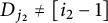 $D_{j_2}\neq [i_2-1]$
is natural. Suppose that D has a column
 $D_j=[m]$
. Such a column is called a standard interval in [Reference Mészáros, Setiabrata and St Dizier23]. Then there is only one choice of
 $C_j$
such that
 $C_j\leq D_j$
, namely,
 $C_j=D_j=[m]$
. So the diagram
 $D^{\prime }$
obtained by removing
 $D_j$
from D inherits all information of D in the sense that
 $\chi _{D}(x)=x_1\cdots x_m\, \chi _{D^{\prime }}(x)$
. So, to prove Theorem 1.1, we may without loss of generality require that D has no standard intervals.
Proof of Lemma 3.3
The assertion is trivial when
 $k=1$
. Assume now that
 $k\geq 2$
. Suppose to the contrary that
 $i_2\leq d_{k-1}$
. We shall deduce the contradiction that
 ${D_{j_2}=[i_2-1]}$
. Since
 $D_{j_1}$
and
 $D_{j_2}$
lie in distinct regions, we have
 $i_1<i_2$
. Our aim is to verify that any box in column
 $j_2$
, lying below row
 $i_2$
, contains a crossing. There are two cases.
Case 1: The box
 $(i_2, j_1)$
belongs to
 $D_{j_1}$
. In this case, we have
 $d_k>i_2$
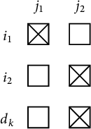
. To avoid the configuration
 $(D)$
in Figure 1, the box
 $(d_k, j_2)$
must contain a crossing, as illustrated in Figure 7.
An illustration for the proof of Case 1.

Consider the box
 $(i, j_2)$
with
 $i>d_k$
. Since each box in column
 $j_1$
, lying below row
 $d_k$
, contains a crossing, to avoid the configuration
 $(E)$
in Figure 1, the box
 $(i, j_2)$
must contain a crossing.
It remains to consider the box
 $(r, j_2)$
with
 $i_2<r<d_k$
. We assert that
 $(r, j_2)\not \in D_{j_2}$
. Suppose otherwise that
 $(r, j_2)\in D_{j_2}$
. If
 $(r, j_1)$
belongs to
 $D_{j_1}$
, then the boxes of D in rows
 $\{i_1, i_2, r\}$
and columns
 $\{j_1, j_2\}$
form the configuration
 $(D)$
in Figure 1, and if
 $(r, j_1)$
does not belong to
 $D_{j_1}$
, then the boxes of D in rows
 $\{i_1, i_2, r, d_p\}$
and columns
 $\{j_1, j_2\}$
form the configuration by swapping the columns of
 $(F)$
in Figure 1. In either case, we are led to a contradiction. This concludes the assertion.
Case 2: The box
 $(i_2, j_1)$
contains a crossing. In this case, we have
 $d_{k-1}>i_2$
. To avoid the configuration
 $(B)$
in Figure 1, the box
 $(d_{k-1}, j_2)$
must contain a crossing. Moreover, to avoid the configuration
 $(A)$
in Figure 1, any box in column
 $j_2$
, which lies below row
 $d_{k-1}$
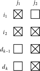
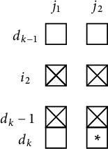
, contains a crossing. The boxes in rows
 $\{i_1, i_2, d_{k-1}, d_k\}$
and columns
 $\{j_1, j_2\}$
look as depicted in Figure 8.
An illustration for the proof of Case 2.

We still need to check that any box in column
 $j_2$
, which lies between row
 $i_2$
and row
 $d_{k-1}$
, contains a crossing. Suppose otherwise that there exists a box
 $(i, j_2)$
with
 $i_2<i<d_{k-1}$
belonging to
 $D_{j_2}$
. Consider the box
 $(i, j_1)$
. If it belongs to
 $D_{j_1}$
, then the boxes in rows
 $\{i_1,i_2, i, d_{k-1}\}$
and columns
 $\{j_1, j_2\}$
would form the configuration
 $(B)$
in Figure 1, and otherwise, the boxes in rows
 $\{i_2, i, d_{k-1}\}$
and columns
 $\{j_1, j_2\}$
would form the configuration by swapping the columns of
 $(A)$
in Figure 1. This verifies that any box
 $(i, j_2)$
with
 $i_1<i<d_{p-1}$
contains a crossing. So the proof is complete.
Lemma 3.4 Take the same assumptions as in Lemma 3.3 (so
 $i_2>d_{k-1}$
).
-
(1) If
$i_2<d_k-1$
, then
$D_{j_2}=[i_2-1]\cup \{d_k\}$
. -
(2) If
$i_2=d_k-1$
, then
$[i_2-1]\cup \{d_k\} \subseteq D_{j_2}$
.




Proof Keep in mind that
 $i_2>d_{k-1}$
.
(1) First, to avoid the configuration obtained by swapping the columns of
 $(A)$
in Figure 1, the box
 $(d_k-1, j_2)$
must contain a crossing. So the boxes in rows
 $\{d_{k-1}, i_2, d_k-1, d_k\}$
and columns
 $\{j_1, j_2\}$
are as illustrated in Figure 9.
An illustration for the proof of (1).

For the same reason as above, any box in column
 $j_2$
, lying between row
 $i_2$
and row
 $d_k-1$
, contains a crossing. Let us look at the box
 $(d_k, j_2)$
. We assert that this box belongs to
 $D_{j_2}$
. Suppose otherwise that
 $(d_k, j_2)$
contains a crossing. To avoid the configuration by swapping the columns of
 $(A)$
in Figure 1, any box in column
 $j_2$
lying below row
 $d_k$
contains a crossing. This, along with the above analysis, implies that
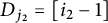 $D_{j_2}=[i_2-1]$
, contradicting the assumption that
 $D_{j_2}\neq [i_2-1]$
. So the assertion is verified.
Now, because
 $(d_k, j_2)\in D_{j_2}$
, any box
 $(i, j_2)$
with
 $i>d_k$
contains a crossing since otherwise the boxes in rows
 $\{i_2, d_k-1, d_k, i\}$
and columns
 $\{j_1, j_2\}$
would yield the configuration by swapping the columns of
 $(C)$
in Figure 1. This shows that
 $D_{j_2}=[i_2-1]\cup \{d_k\}$
.
(2) We need to check that
 $(d_k, j_2)\in D_{j_2}$
. Suppose otherwise that
 $(d_k, j_2)\not \in D_{j_2}$
. Since
 $D_{j_2}\neq [i_2-1]$
, there exists a box
 $(i, j_2)$
with
 $i>d_k$
belonging to
 $D_{j_2}$
. Then the subdiagram, restricted to rows
 $\{d_k-1, d_k, i\}$
and columns
 $\{j_1, j_2\}$
, becomes the configuration
 $(A)$
in Figure 1, leading to a contradiction.
4 Proof of Theorem 1.1
To complete the proof of Theorem 1.1, by Proposition 2.1, it is equivalent to showing that when
 $D=(D_1,\ldots , D_n)$
is multiplicity-free, the eigenspace
 $$\begin{align*}\mathrm{Span}_{\mathbb{C}}\left\{\mathrm{det}\left(Y_{D}^C\right)\colon C\leq D, \, x^C=x^a\right\} \end{align*}$$
has dimension one. We do this by showing that
 $\mathrm {det}\left (Y_{D}^C\right )=\mathrm {det}\left (Y_{D}^{C^{\prime }}\right )$
for
 $C, C^{\prime }\leq D$
with
 $x^C=x^{C^{\prime }}$
. In light of Proposition 2.2, this will be achieved by establishing a bijection between the sets
 $\mathcal {F}_{D}(C)$
and
 $\mathcal {F}_{D}(C^{\prime })$
which preserves both the sign and the weight.
Theorem 4.1 Let
 $D=(D_1,\ldots , D_n)$
be a normalized multiplicity-free diagram, and let
 $C=(C_1,\ldots , C_n) $
and
 $ C^{\prime }=(C_1^{\prime },\ldots , C^{\prime }_n)$
be two distinct diagrams, that are less than or equal to D, such that
 $x^C=x^{C^{\prime }}$
. Then there is a sign- and weight-preserving bijection between the sets
 $\mathcal {F}_{D}(C) $
and
 $\mathcal {F}_{D}(C^{\prime })$
.
Without loss of generality, we may make the following extra assumptions on D:
-
(C 1): each column in
$[n]\times [n]$
has at least two crossings; -
(C 2): D has no column of the form
$[m]$
where
$m\geq 1$
.


The reasons for (C 1) and (C 2) have been explained, respectively, in the beginning of Section 3.2 and below Lemma 3.3.
The construction of the bijection is an iterative procedure, based on an operation, denoted
 $\Phi $
, acting on flagged fillings. The operation depends only on
 $D, C,$
and
 $C^{\prime }$
. Roughly speaking, for
 $F\in \mathcal {F}_{D}(C)$
, the operation
 $\Phi $
interchanges the columns of F by sliding certain entries along the same rows. After applying
 $\Phi $
, we get a new flagged filling
 $\Phi (F)$
, which is “closer” to a flagged filling in
 $\mathcal {F}_{D}(C^{\prime })$
in the sense that there are more columns whose entries match the subsets in
 $C^{\prime }$
. Then we replace F by a flagged filling, denoted
 $\hat {\Phi }(F)$
, which is obtained from
 $\Phi (F)$
by ignoring certain columns that have been adjusted by
 $\Phi $
, and we continue to apply
 $\Phi $
to
 $\hat {\Phi }(F)$
. Eventually, we arrive at a flagged filling belonging to
 $\mathcal {F}_{D}(C^{\prime })$
, which is defined as the image of F.
The description of
 $\Phi $
will be distinguished into three cases, depending on the configuration of the first region of D. Specifically, according to Lemma 3.2, each region of D is one of the following three types: it contains
-
(R 1): only Type I columns, or
-
(R 2): Type I columns followed by some copies of a Type II column, or
-
(R 3): Type I columns followed by exactly one Type III column.
In the remainder of this section, let
 $F=(F_1,\ldots , F_n)$
be any fixed filling in
 $\mathcal {F}_D(C)$
. Our task is to construct
 $\Phi (F)$
, as well as
 $\hat {\Phi }(F)$
obtained from
 $\Phi (F)$
by ignoring some specific columns.
4.1 The first region of D is of Type (R 1)
In this case, the first region of D contains only Type I columns. Suppose that there are m columns in the first region. We may further suppose that for
 $1\leq j\leq m$
,
 $D_j$
is not empty (since empty columns can be obviously ignored). Recall that D satisfies the requirement (C 2) given below Theorem 4.1. Therefore, for
 $1\leq j\leq m$
, the signature of
 $D_j$
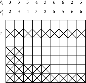
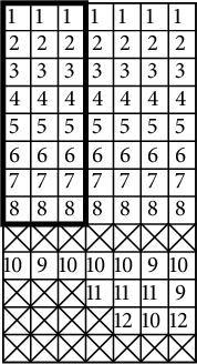
is positive. As an illustration, Figure 10 lists the columns in the first region. Here, we have erased some rows, lying on the bottom, which contain only crossings.
Columns in a Type (R 1) region and their labels.

To describe the operation
 $\Phi $
, we label the m columns in two ways. Suppose that the first crossing in each column is in row r. Let
 $1\leq j\leq m$
. Assume that
 $(n_j, j)$
is the box right above the second crossing in column j (which is the lowest box of
 $D_j$
). Note that
 $n_1\leq n_2\leq \cdots \leq n_m$
. For the region in Figure 10, we have
 $m=9$
and
 $(n_1,\ldots , n_9)=(3,3,5,5,5,6,6,6,6)$
. Observe that
 $C_j=[{n}_j]\setminus \{\ell _j\}$
for some
 $r\leq \ell _j \leq {n}_j$
, and
 $C_j^{\prime }=[{n}_j]\setminus \{\ell _j^{\prime }\}$
for some
 $r\leq \ell _j^{\prime } \leq {n}_j$
. By assigning
 $D_j$
with a label
 $\ell _j$
or
 $\ell _j^{\prime }$
, we obtain two kinds of labelings for the m columns. See Figure 10 for an illustration of the labelings, from which we could recover
 $C_j$
and
 $C^{\prime }_j$
.
Lemma 4.2 As multisets,
 $\{\ell _1,\ldots , \ell _m\}$
is the same as
 $\{\ell _1^{\prime },\ldots , \ell _m^{\prime }\}$
.
Proof For notational simplicity, we denote
 $p=n_m$
. Write
 $$\begin{align*}x^C=x^{C^{\prime}}=x_1^{a_1}\cdots x_p^{a_p}\,x_{p+1}^{a_{p+1}}\cdots x_n^{a_n}. \end{align*}$$
Consider the factor
 $x_1^{a_1}\cdots x_p^{a_p}$
. It can be seen that
 $$ \begin{align*} x_1^{a_1}\cdots x_p^{a_p}&=\frac{\prod_{j=1}^{m}x_1\cdots x_{n_j}}{x_{\ell_1}\cdots x_{\ell_m}}\prod_{j={m+1}}^n\prod_{t\in C_j \atop 1\leq t\leq p} x_t \\ &=\frac{\prod_{j=1}^{m}x_1\cdots x_{n_j}}{x_{\ell_1^{\prime}}\cdots x_{\ell_m^{\prime}}}\prod_{j={m+1}}^n\prod_{t\in C_j^{\prime} \atop 1\leq t\leq p} x_t. \end{align*} $$
By Lemma 3.3, for
 $m+1\leq j\leq n$
, the first crossing in column j is strictly lower than row
 $p-1$
, and thus we have
 $[p-1]\subseteq D_j$
, and hence
 $[p-1]\subseteq C_j$
and
 $[p-1]\subseteq C_j^{\prime }$
. Therefore,
 $$ \begin{align*} x_1^{a_1}\cdots x_p^{a_p}&=\frac{\prod_{j=1}^{m}x_1\cdots x_{n_j}}{x_{\ell_1}\cdots x_{\ell_m}}(x_1\cdots x_{p-1})^{n-m}\prod_{j={m+1}}^n\prod_{p\in C_j} x_p \\ &=\frac{\prod_{j=1}^{m}x_1\cdots x_{n_j}}{x_{\ell_1^{\prime}}\cdots x_{\ell_m^{\prime}}}(x_1\cdots x_{p-1})^{n-m}\prod_{j={m+1}}^n\prod_{p\in C_j^{\prime}} x_p. \end{align*} $$
From the above, we know that
 $\{m+1\leq j\leq n\colon p\in C_j\}$
and
 $\{m+1\leq j\leq n\colon p\in C_j^{\prime }\}$
have the same cardinality. So we have
 $x_{\ell _1}\cdots x_{\ell _m}=x_{\ell _1^{\prime }}\cdots x_{\ell _m^{\prime }}$
, which justifies
 $\{\ell _1,\ldots , \ell _m\}=\{\ell _1^{\prime },\ldots , \ell _m^{\prime }\}$
as multisets.
The operation
 $\Phi $
will be performed on the columns of F in the first region, based on a column-interchanging procedure. Let
 $1\leq j_{1}<j_{2}\leq m$
. Note that if
 $(i, j_1)$
is a box of
 $F_{j_1}$
, then
 $(i, j_2)$
is a box of
 $F_{j_2}$
. We say that
 $F_{j_1}$
and
 $F_{j_2}$
are interchangeable if the resulting filling by swapping the entries in the same rows of
 $F_{j_1}$
and
 $F_{j_2}$
(leaving the entries of
 $F_{j_2}$
below row
 $n_{j_1}$
unchanged) is still a flagged filling. Equivalently, the entries of
 $F_{j_1}$
have no intersection with the entries of
 $F_{j_2}$
that lie below row
 $n_{j_1}$
.
Lemma 4.3 If
 $\ell _{j_2}\leq n_{j_1}$
, then
 $F_{j_1}$
and
 $F_{j_2}$
are interchangeable.
Proof Recall that for
 $1\leq j\leq m$
,
 $C_j=[n_j]\setminus \{\ell _j\}$
. When
 $\ell _{j_2}\leq n_{j_1}$
, the elements in the interval
 $[n_{j_1}+1, n_{j_2}]$
all belong to
 $C_{j_2}$
, and they occupy the boxes of
 $F_{j_2}$
below row
 $n_{j_1}$
. So, after the column-interchanging, the resulting filling is still a flagged filling.
We can now describe the construction of
 $\Phi (F)$
in the Type (R 1) case.
Step 1. Denote
 $c{\kern-1pt}={\kern-1pt}\max \{\ell _1,\ldots , \ell _m\}$
. Let
 $A{\kern-1pt}={\kern-1pt}\{1\leq j\leq m\colon \ell _j{\kern-1pt}={\kern-1pt}c\}$
,
 $B{\kern-1pt}={\kern-1pt}\{1\leq j\leq m\colon \ell _j^{\prime }=c\}$
and
 $S=A\cap B$
. By Lemma 4.2, we have
 $|A|=|B|$
. Assume that
 $A\setminus S=\{j_1<\cdots <j_t\}$
and
 $B\setminus S=\{j_1^{\prime }<\cdots <j_t^{\prime }\}$
. For every
 $1\leq s\leq t$
, swap the entries in the same rows of
 $F_{j_s}$
and
 $F_{j_s^{\prime }}$
(clearly, this is independent of the order of s).
We explain that after Step 1, the resulting filling is also a flagged filling. Consider two cases:
 $j_s>j_s^{\prime }$
and
 $j_s<j_s^{\prime }$
. In the former case, we have
 $\ell _{j_s}=c=\ell ^{\prime }_{j^{\prime }_{s}}\leq n_{j^{\prime }_{s}}$
, and in the latter case, we have
 $\ell _{j_s^{\prime }}<c=\ell _{j_s}\leq n_{j_s}$
. Both cases satisfy the requirement in Lemma 4.3, and thus
 $F_{j_s}$
and
 $F_{j_s^{\prime }}$
are interchangeable.
Step 2. After Step 1, the columns labeled with c are indexed by the set B. Ignore such columns, and then return to Step 1 where the operation is applied to the remaining columns in the first region.
The above algorithm eventually terminates. Define
 $\Phi (F)$
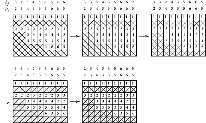
to be the resulting flagged filling. Figure 11 gives an illustration of the construction of
 $\Phi $
. Note that for
 $1\leq j\leq m$
, the label of the j-th column in
 $\Phi (F)$
is equal to
 $\ell _j^{\prime }$
.
An illustration of the construction of
 $\Phi $
in the Type (R 1) case.

Assume that
 $\Phi (F)=(F^{\prime }_1,\ldots , F_n^{\prime })$
. For
 $1\leq j\leq m$
, the set of entries in
 $F_j^{\prime }$
is equal to
 $C_j^{\prime }$
, while for
 $m<j\leq n$
, we have
 $F_j^{\prime }=F_j$
. This means that
 $\Phi (F)$
is “closer” to a filling in
 $\mathcal {F}_D(C^{\prime })$
. We set
 $\hat {\Phi }(F)$
to be the flagged filling obtained from
 $\Phi (F)$
by ignoring the columns in the first region.
4.2 The first region of D is of Type (R 2)
Still, let
 $(D_1,\ldots , D_m)$
be the columns of D in the first region. As in Section 4.1, we assume that each
 $D_j$
for
 $1\leq j\leq m$
is not empty. We also adopt the notation
 $n_j$
which means that
 $(n_j,j)$
is the box right above the second crossing in column j. Note that when
 $D_j$
is a column of Type II,
 $(n_j,j)$
is not the lowest box of
 $D_j$
.
Imitating Section 4.1, we label each column
 $D_j$
for
 $1\leq j\leq m$
in two ways, also denoted by
 $\ell _j$
and
 $\ell _j^{\prime }$
. Let us first define
 $\ell _j$
. Consider
 $[n_j]\setminus C_j$
. If
 $D_j$
is of Type I, then
 $[n_j]\setminus C_j$
contains exactly a single element, just as in Section 4.1. While, if
 $D_j$
is of Type II, then
 $[n_j]\setminus C_j$
either contains a single element or is the empty set. Clearly,
 $[n_j]\setminus C_j=\emptyset $
if and only if
 $C_j=[n_j]$
. When
 $[n_j]\setminus C_j$
contains a single element, let
 $\ell _j$
be this element, and when
 $[n_j]\setminus C_j=\emptyset $
, let
 $\ell _j=\emptyset $
. In completely the same manner, we may define
 $\ell ^{\prime }_j$
with respect to
 $C^{\prime }_j$
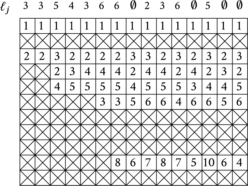
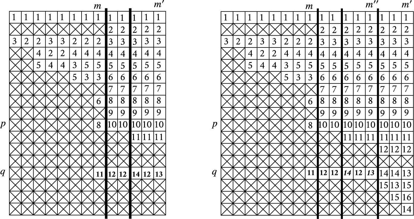
. Figure 12 illustrates the columns, as well as their labels, in the first (Type (R 2)) region of a filling F in
 $\mathcal {F}_{D}(C)$
.
Lemma 4.4 As multisets,
 $\{\ell _1,\ldots , \ell _m\}$
is the same as
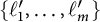 $\{\ell _1^{\prime },\ldots , \ell _m^{\prime }\}$
.
An illustration of columns and their labels in a Type (R 2) region.

Proof The proof is similar to (actually slightly easier than) that of Lemma 4.2. Let
 $p=n_m$
, and write
 $x^C=x^{C^{\prime }}=x_1^{a_1}\cdots x_p^{a_p}\,x_{p+1}^{a_{p+1}}\cdots x_n^{a_n}.$
By Lemma 3.3, for
 $m+1\leq j\leq n$
, the first crossing in column j is lower than row p, which implies
 $[p]\subseteq D_j$
and in turn
 $[p]\subseteq C_j$
and
 $[p]\subseteq C_j^{\prime }$
. Now, we see that
 $$ \begin{align*} x_1^{a_1}\cdots x_p^{a_p}=\frac{\prod_{j=1}^{m}x_1\cdots x_{n_j}}{x_{\ell_1}\cdots x_{\ell_m}}(x_1\cdots x_{p})^{n-m} =\frac{\prod_{j=1}^{m}x_1\cdots x_{n_j}}{x_{\ell_1^{\prime}}\cdots x_{\ell_m^{\prime}}}(x_1\cdots x_{p})^{n-m}, \end{align*} $$
where we set
 $x_{\emptyset }=1$
. It follows that
 $x_{\ell _1}\cdots x_{\ell _m}=x_{\ell _1^{\prime }}\cdots x_{\ell _m^{\prime }}$
, and so
 $\{\ell _1,\ldots , \ell _m\}=\{\ell _1^{\prime },\ldots , \ell _m^{\prime }\}$
as multisets.
Unlike Section 4.1, the construction of
 $\Phi (F)$
in the Type (R 2) case requires two algorithms. The first algorithm acts on the columns in the first region in the same way as the algorithm in Section 4.1. Here, the label
 $\emptyset $
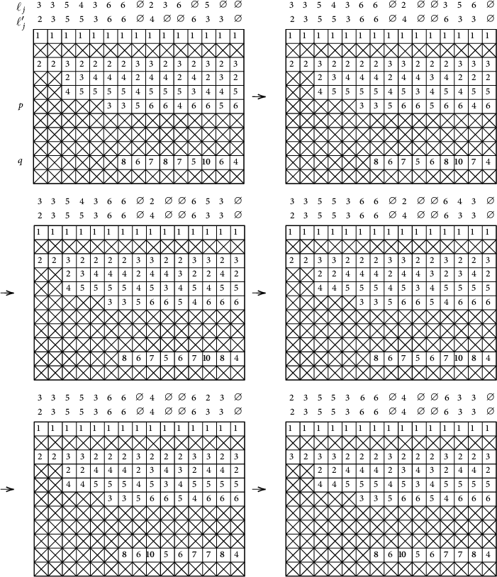
is regarded as the infinity which is greater than any positive integer. This procedure will be best understood via an example in Figure 13.
Illustration of the first algorithm in the Type (R 2) case.

After applying the above algorithm, the label of
 $D_j$
for
 $1\leq j\leq m$
becomes
 $\ell _j^{\prime }$
. Denote by
 $F^{(1)}$
the resulting flagged filling. Suppose that
 $F^{(1)}=(F^{(1)}_1,\ldots , F^{(1)}_n)$
belongs to
 $\mathcal {F}_{D}(C^{(1)})$
where
 $C^{(1)}=(C^{(1)}_1,\ldots , C^{(1)}_n)$
. Clearly, we have
 $F^{(1)}_j=F_j$
for
 $m< j\leq n$
. For
 $1\leq j\leq m$
, we have
 $C_j^{(1)}=C_j^{\prime }$
when
 $D_j$
is either a Type I column or a Type II column labeled with
 $\emptyset $
.
We still need to consider the Type II columns in the first region whose labels are not
 $\emptyset $
. Let
 $p=n_m$
. By (2) in Lemma 3.2, the lowest boxes in the Type II columns lie in the same row, say row q. Our next task is to adjust the entries in row q that are greater than p. Note that such entries lie in the Type II columns whose labels are not
 $\emptyset $
. In Figure 13, the entries greater than p lying in row q are displayed in boldface, where
 $p=6$
and
 $q=10$
.
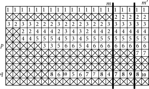
To deal with the entries in row q that are greater than p, we need additionally to invoke the regions (after the first region) whose first crossings lying in or above row
 $q-1$
. According to Lemma 3.3, the first crossing in each such region is below row p. Suppose that there are
 $k-1$
(
 $k\geq 1$
) such regions. By Lemma 3.4, each column in these regions contains a box of D in row q. Together with the first region, we next consider the first k regions of D. Assume that the first k regions have a total of
 $m^{\prime }$
columns. For
 $1\leq r\leq k$
, assume that the first crossing in the r-th region is in row
 $i_r$
. Note that
 $1\leq i_1<\cdots <i_k\leq q-1.$
The description of the second algorithm will be divided into two cases, according to the relative values of
 $i_k$
and
 $q-1$
.
Case 1.
 $i_k<q-1$
. By (1) in Lemma 3.4, for
 $m<j\leq m^{\prime }$
,
 $D_j$
has exactly one box below the first crossing which lies in row q. The second algorithm acts on the entries in the row q of
 $F^{(1)}$
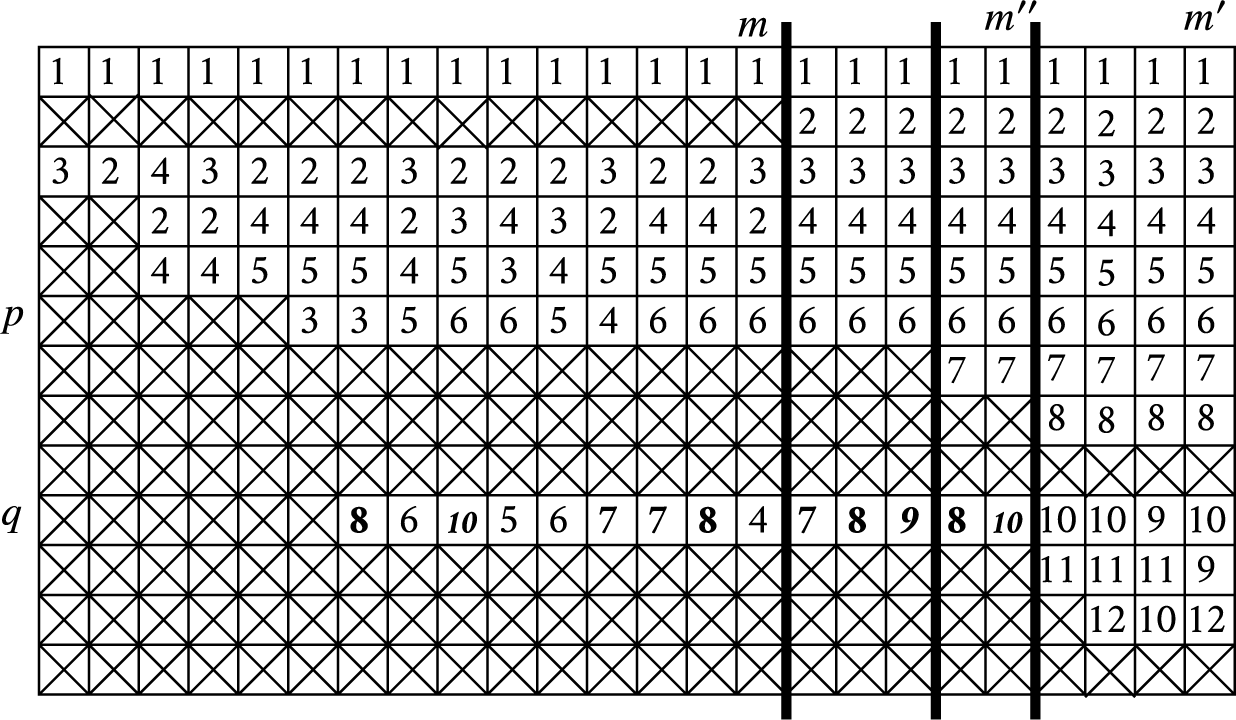
, restricted to the first k regions, that are greater than p. Suppose that there are d such entries, say
 $(a_1,\ldots , a_d)$
listed from left to right, and that for
 $1\leq t\leq d, \ a_t$
lies in column
 $j_t$
. An illustration is given in Figure 14, where we set
 $k=3$
and
 $d=10$
, and the entries in
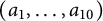 $(a_1,\ldots , a_{10})$
are drawn in boldface.
An illustration for Case 1 in the second algorithm.

Notice that for
 $1\leq t\leq d$
,
 $a_t$
can be obviously read off from
 $C^{(1)}_{j_t}$
. To be precise, suppose that
 $D_{j_t}$
is in the r-th region. For
 $r=1$
,
 $a_t$
is the unique element in
 $C^{(1)}_{j_t}$
that is greater than p, while for
 $2\leq r\leq k$
,
 $a_t$
is the unique element in
 $C^{(1)}_{j_t}=C_{j_t}$
that is greater than or equal to
 $i_r$
. We define
 $b_t$
by replacing
 $C^{(1)}_{j_t}$
with
 $C^{\prime }_{j_t}$
.
Lemma 4.5 As multisets, we have
 $\{a_1,\ldots , a_d\}=\{b_1,\ldots , b_d\}$
.
Proof Note that the first crossing in any column of D after the k-th region lie in or below row q. The proof is then done by using completely similar arguments to those for Lemma 4.2.
Define
 $\Phi (F)$
to be the flagged filling obtained from
 $F^{(1)}$
by replacing the entry
 $a_t$
with
 $b_t$
for
 $1\leq t\leq d$
. Write
 $\Phi (F)=(F_1^{\prime },\ldots , F_n^{\prime })$
. Then, for
 $1\leq j\leq m^{\prime }$
, the set of entries in
 $F_j^{\prime }$
is equal to
 $C_j^{\prime }$
, while for
 $m^{\prime }<j\leq n$
, we have
 $F_j^{\prime }=F_j$
. Let
 $\hat {\Phi }(F)$
be obtained from
 $\Phi (F)$
by ignoring the first
 $m^{\prime }$
columns.
Case 2.
 $i_k=q-1$
. By (2) in Lemma 3.4, each column of D in the k-th region has a box in row q. Focus on the columns of
 $F^{(1)}$
in the first
 $k-1$
regions (columns in the k-th region will be kept unchanged). We consider the entries in the q-th row. In the same way as in Case 1, we may define the sequences
 $(a_1,\ldots , a_d)$
and
 $(b_1,\ldots , b_d)$
. See Figure 15 for an illustration, where
 $k=4$
, and the entries in the sequence
 $(a_1,\ldots , a_d)$
are shown in boldface.
An illustration for Case 2 in the second algorithm.

In this figure, we use italics to distinguish the entries equal to
 $q-1$
or q, and the reason for this will be clear later.
Lemma 4.6 The multiset obtained from
 $\{a_1,\ldots , a_d\}$
by removing the elements equal to
 $q-1$
or q is the same as the multiset obtained from
 $\{b_1,\ldots , b_d\}$
by removing the elements equal to
 $q-1$
or q.
Proof The proof is the analogous to that for Lemma 4.4, and so is omitted.
It should be pointed out that the subset of
 $\{a_1,\ldots , a_d\}$
consisting of
 $q-1$
and q is not necessarily equal to the subset of
 $\{b_1,\ldots , b_d\}$
consisting of
 $q-1$
and q, because of the existence of the k-th region (namely, the region with topmost crossings in row
 $q-1$
).
We construct
 $(a_1^{\prime },\ldots , a_d^{\prime })$
by reordering the elements of
 $(a_1,\ldots , a_d)$
as follows. First, shuffle the subword including elements not equal to
 $q-1$
or q and the subword including
 $q-1$
and q, such that the elements not equal to
 $q-1$
or q occupy the same positions as in
 $(b_1,\ldots , b_d)$
(this is well defined according to Lemma 4.6). Then, rearrange the elements not equal to
 $q-1$
or q such that they have the same order as in
 $(b_1,\ldots , b_d)$
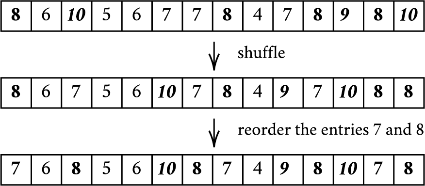
. For example, assuming
 $(b_1,\ldots , b_d)=(7,8,9,8,7,9,8,10,7,8)$
, the sequence
 $(a_1,\ldots , a_d)$
in Figure 15 will be changed into
 $(a_1^{\prime },\ldots , a_d^{\prime })$
as illustrated in Figure 16.
An illustration from
 $(a_1,\ldots , a_d)$
to
 $(a_1^{\prime },\ldots , a_d^{\prime })$
.

Define
 $\Phi (F)$
as the flagged filling obtained from
 $F^{(1)}$
by replacing the entry
 $a_t$
with
 $a_t^{\prime }$
for
 $1\leq t\leq d$
. Write
 $\Phi (F)=(F_1^{\prime },\ldots , F_n^{\prime })$
. Suppose that there are
 $m^{\prime \prime }$
columns in the first
 $k-1$
regions. For
 $m^{\prime \prime }<j\leq n$
, we clearly have
 $F_j^{\prime }=F_j$
. While, for
 $1\leq j\leq m^{\prime \prime }$
, when
 $F_j^{\prime }$
does not contain
 $q-1$
or q, the set of entries in
 $F_j^{\prime }$
is equal to
 $C_j^{\prime }$
.
The construct of
 $\hat {\Phi }(F)$
is as follows. First, ignore the “well-behaved” columns, namely, the columns in the first
 $k-1$
regions of
 $\Phi (F)$
not containing
 $q-1$
or q. Then, merge the remaining columns (namely, columns containing
 $q-1$
or q) into the k-th region, in such a way that we erase all crossings above row
 $q-1$
. Specifically, for
 $1\leq j\leq m^{\prime \prime }$
, if
 $F^{\prime }_j$
contains
 $q-1$
or q, then we replace
 $D_j$
by
 $D_j\cup [q-2]=[q-2]\cup \{q\}$
, and correspondingly, we replace
 $C^{(1)}_j$
and
 $C^{\prime }_j$
, respectively, by
 $C^{(1)}_j\cup [p-2]$
and
 $C^{\prime }_j\cup [p-2]$
. For the portion in Figure 15, the illustration that the columns containing
 $q-1$
or q are merged into the k-th region is given in Figure 17.
The merging procedure for Figure 15.

We remark that all the entries above row
 $q-1$
in the merged columns, which are framed by lines in boldface in Figure 17, will keep unchanged in the next round of the iteration. So the merging operation merely plays a role that the columns in the first
 $k-1$
regions, containing
 $q-1$
or q, are viewed as columns in the k-th region, so that our algorithms could be implemented in the next iteration.
4.3 The first region of D is of Type (R 3)
In this case, the construction of
 $\Phi (F)$
as well as
 $\hat {\Phi }(F)$
is nearly the same as that for the Type (R 2) case in Section 4.2. So the description will be sketched. All but one of the notation (namely, the notation p) will be fully consistent with what we used in Section 4.2.
Let
 $(D_1,\ldots , D_m)$
be the first region of D. Keep in mind that
 $D_j$
for
 $1\leq j<m$
are Type I columns, and
 $D_m$
is a Type III column. For
 $1\leq j\leq m$
, let
 $n_j$
be the row index such that
 $(n_j, j)$
is the box right above the second crossing in column j. Note that
 $[n_j]\setminus C_j$
(respectively,
 $[n_j]\setminus C_j^{\prime }$
) contains a single element, or is equal to
 $\emptyset $
(this possibly occurs only when
 $j=m$
), which is defined as the label
 $\ell _j$
(respectively,
 $\ell _j^{\prime }$
).
Perform the first algorithm as in Section 4.2 to interchange the columns of F in the first region. The resulting flagged filling is denoted
 $F^{(1)}=(F^{(1)}_1,\ldots , F^{(1)}_n)$
. Suppose that
 $F^{(1)}$
belongs to
 $\mathcal {F}_{D}(C^{(1)})$
where
 $C^{(1)}=(C^{(1)}_1,\ldots , C^{(1)}_n)$
. Then
 $C^{(1)}_j=C_j^{\prime }$
for
 $1\leq j<m$
. Moreover, one has
 $F^{(1)}_j=F_j$
for
 $m< j\leq n$
. We next deal with the column
 $F^{(1)}_m$
, parallel to what we do in the second algorithm in Section 4.2.
Since
 $D_m$
is a Type III column, there are at least two boxes of
 $D_m$
lying below the second crossing. Let
 $p<q$
be the row indices such that
 $(p,m)$
and
 $(q,m)$
are the lowest two boxes of
 $D_m$
. Unlike in Section 4.2, we will no longer have the relation
 $p=n_m$
. Suppose that there are k regions whose first crossings lie in or above row
 $q-1$
.
For
 $1\leq r\leq k$
, assume that the first crossing in the r-th region is in row
 $i_r$
. We consider two cases.
Case 1.
 $i_k<q-1$
. The left picture in Figure 18 is an instance of this case. Define
 $\Phi (F)$
and
 $\hat {\Phi }(F)$
by applying the same procedure as in Case 1 of Section 4.2.
Illustrations for Type (R 3) case with
 $i_k<q-1$
or
 $i_k=q-1$
.

Case 2.
 $i_k=q-1$
. This case is demonstrated in the right picture in Figure 18. Define
 $\Phi (F)$
and
 $\hat {\Phi }(F)$
by applying the same procedure as in Case 2 of Section 4.2.
4.4 Proof of Theorem 4.1
Starting with
 $F\in \mathcal {F}_D(C)$
, we iterate the operation
 $\Phi $
and eventually arrive at a flagged filling, denoted
 $\Omega (F)$
, in
 $\mathcal {F}_D(C^{\prime })$
. We explain that
 $\Omega $
is a bijection from
 $\mathcal {F}_D(C)$
to
 $\mathcal {F}_D(C^{\prime })$
that preserves both the sign and weight. To check that
 $\Omega $
is a bijection, the key is to make clear which and how columns are swapped in each step. By our construction, this only depends on the diagrams
 $D, C,$
and
 $ C^{\prime }$
, independent of the flagged filling F. Moreover, it is easy to see that the operation in each step in Sections 4.1–4.3 may be reversed.
We next check that
 $\Omega $
preserves the sign and weight of F. It suffices to verify that F and
 $\Phi (F)$
have the same sign and weight. Since the entries (if moved) are slid in the same row, we have
 $y^{F}=y^{\Phi (F)}$
. To see that F and
 $\Phi (F)$
have the same sign, recall that there are two kinds of operations in our construction.
-
(1) Two columns
$F_{j_1}$
and
$F_{j_2}$
(
$j_1<j_2$
) of F are exchanged. Suppose that
$F_{j_1}$
has column reading word
$u=a_1 a_2\cdots a_s$
, and
$F_{j_1}$
has column reading word
$v=b_1 b_2\cdots b_t$
. Note that
$s\leq t$
. After column-exchanging, the reading words in columns
$j_1$
and
$j_2$
become
$u^{\prime }=b_1 b_2\cdots b_s$
and
$v^{\prime }=a_1 a_2\cdots a_s \,b_{s+1}\cdots b_t$
, respectively. Notice that any element in
$\{b_{s+1}, \ldots , b_t\}$
is bigger than any element in
$\{a_1,\ldots , a_s\}$
or
$\{b_1,\ldots , b_s\}$
. This implies that
$\mathrm {inv}(u)+\mathrm {inv}(v)=\mathrm {inv}(u^{\prime })+\mathrm {inv}(v^{\prime })$
. -
(2) Some entries in row q are reordered. In this case, the inversion number of each column reading word is unchanged since the moved entries in row q are bigger than any entry above row q in the corresponding columns.


By the above analysis, we obtain that
 $\Omega $
is a sign- and weight-preserving bijection. This allows us to conclude the proof of Theorem 4.1.
Acknowledgements
We would like to thank the anonymous referee for valuable comments and suggestions.
Funding
This work was supported by the National Natural Science Foundation of China (No. 12371329) and the Fundamental Research Funds for the Central Universities (Grant No. 63243072).