Introduction
Since von Helmholtz’s study (von Helmholtz, Reference von Helmholtz1867) in 1867, visuomotor transformation, which is the principal element of human arm reaching movement, has been a subject of extensive investigation (Trommershäuser et al., Reference Trommershäuser, Maloney and Landy2003; Körding & Wolpert, Reference Körding and Wolpert2006; Tassinari et al., Reference Tassinari, Hudson and Landy2006). Visuomotor transformation is considered an important field for explicating the basic control mechanisms of human movement. Identification of an object’s spatial position based on visual input and the transformation of this visual input into a motor output towards the object’s coordinates are essential processes in the human control mechanism (Kawato, Reference Kawato1999). Prism adaptation is frequently used in visuomotor transformation. When a subject performs an arm reaching movement, while his or her visual field is horizontally shifted by using prism glasses, the subject’s arm initially moves significantly away from the target and toward the direction of the visual shift (direct effect). The magnitude of error in the initial movement lessens with the number of trials, and after several attempts, the correct movement toward the target is finally achieved. This process is called prism adaptation. When the same reaching movement is performed after removing the prism glasses, a similar error occurs in the opposite direction. The magnitude of error after removing the prism glasses is called the magnitude of the after effect, and it represents the subject’s degree of prism adaptation (Redding & Wallace, Reference Redding and Wallace1978). A large magnitude of the after effect indicates that a new calibration between the visual input and motor output has been firmly achieved. However, the degree of prism adaptation is not always the same for each subject, and it depends on various situations that can occur during the process of prism adaptation (Norris et al., Reference Norris, Greger, Martin and Thach2001). Redding et al. (1988, 1990) reported that the degree of prism adaptation varies according to the differences in the amounts of proprioceptive and visual sensations. In the recent studies, several investigators have reported that the determination of spatial coordinates required for prism adaptation does not generate coordinates common to visual or proprioceptive sensations, but that the determination is independently performed based on the reliable feedback information (Ernst & Banks, Reference Ernst and Banks2002; Helbig & Ernst, Reference Helbig and Ernst2008).
A probabilistic prediction model for determining movement has been recently proposed from computational model viewpoints (Kersten & Yuille, Reference Kersten and Yuille2003; Ernst & Bülthoff, Reference Ernst and Bülthoff2004; Scheidt & Ghez, Reference Scheidt and Ghez2007). In the field of control systems engineering, estimation of some hidden states using system identification has been also widely used for appropriate motor control in human (Baddeley et al., Reference Baddeley, Ingram and Miall2003; Wolpert, Reference Wolpert2007; Burge et al., Reference Burge, Ernst and Banks2008). A computational model is one approach to prospectively estimate various information processing activities in the brain. An external observation of prism adaptation cannot directly reveal the process of transformation between visual and motor sensations. However, by statistically estimating the state parameters, the processes in which the brain internal model estimates an external state can be known (Rao, Reference Rao1999). Kitazawa et al. (Reference Kitazawa, Kohno and Uka1995) studied the mechanism of the prism adaptation by a lag of the sight for visual feedback. They suggested a discrete model using only two parameters: correction rate and initial error for the adaptation process. His proposal is one of the most definite parametric linear models based on a unique identification. On the other hand, a probabilistic estimation model is well known to sequentially determine the state parameter according to changes in external dynamics (Tin & Poon, Reference Tin and Poon2005; Burge et al., Reference Burge, Girshick and Banks2010; Wei & Körding, Reference Wei and Körding2010). There is a probabilistic model using Kalman filtering for system identification. The Kalman filter model flexibly determines the optimal parameters based on the relationship between the error variance of observation data and the uncertainty of system estimation (Kalman, Reference Kalman1960; Kalman & Bucy, Reference Kalman and Bucy1961). The computational algorithm of Kalman filtering is composed of mathematical frameworks based on Bayesian estimation (Wolpert, Reference Wolpert2007). Bayesian estimation handles the state parameter vectors as a conditional probability distribution and calculates the likelihood function of the optimal parameters (Bayes & Price, Reference Bayes and Price1763). The probabilistic model based on Bayesian estimation has been considered very effective in explaining human intracerebral information processing, such as decision-making and behavior selection (Pouget et al., Reference Pouget, Dayan and Zemel2003; Ma et al., Reference Ma, Beck, Latham and Pouget2006; MacNeilage et al., Reference MacNeilage, Ganesan and Angelaki2008; Zemel et al., Reference Zemel, Dayan and Pouget1998). In a recent study on human reaching movement based on the probabilistic model, Baddeley et al. (Reference Baddeley, Ingram and Miall2003) proposed that the changes occurring in everyday life are better represented as the accumulation of many smaller perturbations contaminated with measurement noise. They tested human performance to follow random fluctuations in the displayed cursor location instead of the hand movements during a pointing task. They manipulated the mapping between the hand and end-point position by adding an artificial drift parameter and observation noise. The several computational models were compared based on the human efficiency levels. They speculated that the efficiency of the human performance appears to be limited by action noise (system errors of the estimation process). In consideration of system errors derived from variations in visuomotor transformation, a modified probabilistic model was also reported. Burge et al. (Reference Burge, Ernst and Banks2008) studied the effects of measurement uncertainty (by blurring the visual feedback) on human reaching movement. They investigated how Kalman filtering model takes into account the statistical systematic errors and the reliability of the observation errors by calculating recalibration rate. For most visual feedback conditions, behavior of human and Kalman filter was similar: Increasing measurement uncertainty caused similar decreases in recalibration rate; alternatively, more variation in systematic error increased recalibration rate.
This study aims to create an optimal model for hidden state estimation and to elucidate the required information processing for identifying an external dynamics. Questions on obtaining a likelihood state estimation remain: how is the plurality of information selected, furthermore, how is uncertain information processed? To address these questions, we set up various perturbations on the visual sensation and measured the prism adaptation process. First, we changed the amount of the visual information in regard to the fingertip trajectory and arrival positions. Next, visual coordinates system was switched from egocentrism coordinates to external coordinates. Furthermore, presentation timing of the images was delayed. Under these conditions, we compared Kalman filtering model and the discrete linear model. We postulated that the linear model can well predict in a certainly feedback information but not be fitting in an uncertainly visual information. The estimation using Kalman model may be well fitting in all conditions. Indeed, it would be beneficial to know a priori how such modeling techniques would differentially predict prism adaptation in distinct feedback conditions. In this study, we hoped to clarify the estimating process based on feedback information for visuomotor transformation from computational model viewpoints.
Materials and methods
Experimental setup
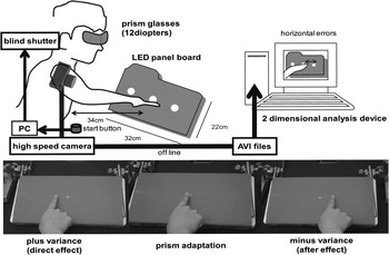
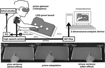
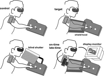
In the experiment, 57 healthy male right-handed students between the ages of 20 and 39 years were used as subjects. The mean age was 29.5 ± 2.3 years old. We explained the purpose and method of this study to each subject based on the Helsinki Declaration and obtained their written consent. We informed them that they could withdraw their consent at any time. The subjects sat in front of a light-emitting diode (LED) panel placed on a desk. The size of the LED panel, which was covered with a green sheet, was 32 × 22 cm. Three LEDs (0.5 cm diameter) were horizontally arranged at the center of the panel at 3.4 cm intervals. Movies of the subject’s reaching movements were taken continuously by a high speed camera (EX-F1; Casio Computer Co., Ltd., Tokyo, Japan), which was installed in the center of the panel’s upper frame (at a height of 22 cm from the top of the desk). The angle of the camera to the panel was 20 deg. The camera’s frame rate was 300 f/s. The image data from the camera were converted into AVI files. Using a coordinate-calibrated two-dimensional motion analysis device (Frame-DIAS IV; DKH Co., Ltd., Tokyo, Japan), the horizontal error between the target LED and subject’s finger position was calculated. The accuracy of the measurement was below ±1.5 mm. In addition, the reaction time and duration for reaching movement were calculated from motion analysis at off line. Fig. 1 shows the experimental setup.
Experimental setup. Each of the subjects placed his or her right index finger at a point 34 cm in front of the panel. The subjects were then instructed to rapidly perform reaching movements to one of the randomly illuminating LED lights. The subjects started reaching movement by turning off the button of the fingertip, and the off signal was sent to the personal computer. The liquid crystalline shutter was operated by the trigger signal. The experimental protocol for prism adaptation was composed of three blocks. In the first block, the subjects performed their reaching movements without wearing prism glasses. In the second block, their movements were performed while wearing prism glasses and produces direct effect of plus variance. In the third block, their movements were again performed with their naked eye and produces after effect of minus variance.
Experimental protocol
Each of the subjects placed his or her right index finger at a point 34 cm in front of the panel. The subjects were then instructed to rapidly perform reaching movements to one of the randomly illuminating LED lights. The experimental protocol for prism adaptation was composed of three blocks. In the first block, the subjects performed their reaching movements without wearing prism glasses. In the second block, their movements were performed while wearing prism glasses. In the third block, their movements were again performed without wearing prism glasses. Thirty trials were conducted for each block, that is, 90 trials in total. The prism glasses allowed a refractive displacement of 12 diopters in the left horizontal direction. The subjects closed their eyes while putting on and removing the prism glasses between blocks. The trials in the next block were initiated immediately after putting on or removing the prism glasses as required. We did not explain the effect of the visual field displacement expected from the use of the prism glasses to the subjects. Therefore, some of the subjects were unaware of the visual field displacement until the end of the experiment. Each LED was controlled by a microcomputer controller (IMTEC Inc., Osaka, Japan). The time required for each subject to finish the experiment was roughly 40 min.
Perturbation of visual feedback
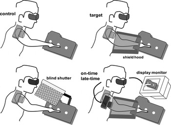
To investigate the effects of various perturbations of visual feedback on prism adaptation, we prepared four test conditions in Fig. 2. For the first condition (called the target condition), the trajectory of the fingertip movement was shielded, and only a reaching error was fed back to the subject based on the difference in position between the fingertip and LED target at the end of the movement. Under this condition, visual information of the fingertip position before and during the movement was not given, and only the proprioceptive sensation during the movement was fed back. For the second condition (called the trajectory condition), although the trajectory of the fingertip movement could be seen, the final reaching error was not fed back. In other words, during a reaching movement, both the visual and proprioceptive sensations were fed back. For the target condition, a homemade black shield hood (made of polypropylene; 55 × 28 × 15–20 cm) was installed at the location where the reaching movement was to be performed. The participants could not egocentrically evaluate the position of their limb to the target. To realize the trajectory condition, a blind shutter (Takei Instruments Co., Ltd., Niigata-city, Japan) installed just in front of the subject was closed immediately before the end of the reaching movement. The liquid crystal shutters were closed by a personal computer used for collection of movement duration. The subjects started reaching movement by turning off the button of the fingertip, and the off signal was sent to the same personal computer, and the liquid crystal shutter operated 200 ms later (Fig. 1). The shutting precision of the liquid crystalline shutter was below 1 ms. The movement duration for all trials was 320 ms or less. When further duration occurred, the data were excluded from count. Referring to the adaptation conditions proposed by Redding and Wallace (Reference Redding and Wallace1988, Reference Redding and Wallace1990), these two conditions were established to restrict the amount of visual feedback information. In the target condition, the visual feedback of the limb position on the visual field was neither available during premovement nor response control, whereas in the trajectory condition, it was available in both phase. Because the feedback methods of sense were different under conditions of these, the sensory mapping for the visuomotor transformation developed a different sensory motor calibration (Prablanc et al., Reference Prablanc, Echallier, Komilis and Jeannerod1979). In our experiment, two more restricted visual feedback conditions were prepared. These conditions were established based on the study reported by Norris et al., (Reference Norris, Greger, Martin and Thach2001). To show the reaching movement to the subject, a digital video camera (HDR-CX560V; Sony Co., Ltd., Tokyo, Japan) with an average bit rate of 9 Mbps was installed along the median line of the subject. The video images were reproduced on a diagonal of 48.1-cm LCD display (LCD Display L-W191; Sharp Co., Ltd., Osaka, Japan) located around 50 cm away from the subject. That is, instead of the space where the subject’s egocentric coordinates (i.e., Euclidean distance from operator to some environmental object/target) (Previc, Reference Previc1998), the subject underwent prism adaptation based on the monitor images, which were converted into external coordinates. Under one condition, the images were reproduced at the same time the reaching movement occurred (which we call on-time condition). Indeed, playback lag was below 1 ms in this condition. This accuracy has been maintained by directly using pass way to monitoring, namely, the digital data have not been stored. In the other condition, the images were reproduced with 220 ms of delay (late-time condition). Captured images were sent to personal computer (R-500; IBM Co., Ltd., New York). After it was stored by a personal computer, the image data were played back by a digital capture board in the form MPEG-2. In this condition, a temporal gap was generated between the visual sensation and the feedback of the motor sensation. We investigated the effects of asynchronism between the visual feedback and motor sensation under this condition. Finally, trials under normal prism adaptation were conducted as a control group. The subjects were randomly divided into five groups. Target was 12 subjects, and trajectory, on-time, and late-time conditions were 10 subjects, respectively. In addition, control was 15 subjects.
Schematic overview of five different visual feedback conditions. Both the trajectory of the fingertip and LED target are visible in control condition. In the target condition, the trajectory of the fingertip movement was shielded, and only a reaching error was fed back to the subject. In the trajectory condition, the trajectory of the fingertip movement was visible but the final reaching error was not fed back. To realize the trajectory condition, a blind shutter installed just in front of the subject was closed immediately (50–100 ms) before the end of the reaching movement. In the on-time condition and the late-time condition, subject underwent prism adaptation based on the monitor images, which were converted into external coordinates. Under on-time condition, the images were reproduced at the same time the reaching movement occurred. In the late-time condition, the images were reproduced with 220 ms of delay.
Comparing models describing prism adaptation
We measured the horizontal error distance between the LED and reaching position of the fingertip in each trial under every condition. To estimate the dynamics of prism adaptation due to the different visual feedbacks, we set up a linear parametric model and a probabilistic model a priori.
Discrete linear model
For the estimation of the linear parametric model, we employed the following discrete linear model proposed by Kitazawa et al. (Reference Kitazawa, Kohno and Uka1995):
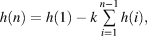
where h represents the horizontal error distance, n is the number of discrete trials, and k indicates the correction parameter coefficient. The correction parameter coefficient represents the feedback weighting effect. Using this simple model, they clearly explained the dynamics of prism adaptation as being due to the different exhibiting times of visual error feedback.
Statistical model using dynamic Bayesian estimation: Kalman filtering
When time series data are observed, these dynamics depend on the state variable of the system. Kalman filtering sequentially obtains the optimal solution from recurrence equations by using a random state variable. Kalman filtering is composed of the following recurrence equations:


In these equations, the state variable  is estimated based on the observation data
 . Moreover, F represents the observation matrix, G is the state transition matrix, and ω and ξ are the observation and system noises following the Gaussian distribution, respectively. Here, the method for updating the state variable
 in the Bayesian estimation framework with normal distribution is considered to be as follows:


The posterior probability distribution,  , of state variable
 is obtained by multiplying the prior probability distribution,
 , of
 , which is estimated at time t, and the likelihood,
 , of observation data
 . In this case, the data likelihood are affected by the reliability of the difference (innovation) between the value of the state estimation and the observation data. The actual state variable,
 , can be obtained by correcting
 , which is predicted from system equation (3) using
 as follows:

where the proportionality coefficient, κ, in the error term is used to adjust the reliability of the innovation using Kalman gain. κ can be obtained as follows:

Kalman gain is the ratio of the variance of an expected value obtained using the state transition of the predicted state variable caused by the system to the variance of the observation data at the next moment in time. Kalman gain creates a tradeoff between the reliability of a system and that of the observation data. For example, when Kalman gain is large, the predicted state variable  is more accurately corrected using the observation data.
Results
The mean of reaction time was 249 ± 11.0 ms in all conditions. Control condition was 247 ms, target condition was 249 ms, trajectory condition was 251 ms, on-time condition was 248 ms, and late-time condition was 252 ms (mean ± s.d.). We show the mean of reaching duration in three blocks in each condition. Control condition was 286 ± 19.4 ms, target condition was 291 ± 17.4 ms, trajectory condition was 296 ± 21.5 ms, on-time condition was 287 ± 22.3 ms, and late-time condition was 289 ± 23.9 ms (mean ± s.d.). None had the significant difference (P > 0.114). The mean of trial taken beyond 320-ms duration was 4.2 trials in each subject. Those data were finally omitted.
Differences between prism effects
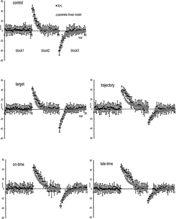
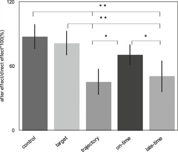
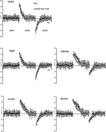
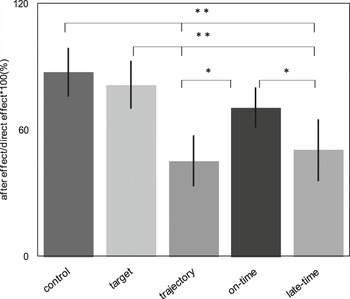
We observed the following tendencies under almost all conditions. We compared the convergent of the error distance by the mean of 10 trials of the latter half through 30 trials at each block. Consequently in block 1, the control element was 2.3 ± 0.7 mm (mean ± s.d.), and the target, trajectory, late-time, and on-time conditions were 2.7 ± 0.5 mm, 3.6 ± 1.0 mm, 3.9 ± 1.7 mm, and 2.9 ± 1.1 mm (mean ± s.d.), respectively. There was a significant difference in between control condition and trajectory and late-time conditions (P < 0.05). In block 2, the visual field was displaced due to the direct effect. The magnitude of error was the largest toward the left side at the initial trial but either gradually or rapidly converged to nearly 0 mm. sequentially, the control condition was 2.4 ± 0.2 mm (mean ± s.d.), and the target, trajectory, late-time, and on-time conditions were 2.9 ± 0.8 mm, 4.0 ± 1.6 mm, 4.3 ± 1.4 mm, and 2.8 ± 1.5 mm (mean ± s.d.), respectively. There was a significant difference in between control condition and trajectory and late-time conditions similarly to block 1 (P < 0.05). In block 3, reverse changes as that in block 2 were observed due to the after effects (Fig. 3). Therefore, the control condition was 2.1 ± 0.5 mm (mean ± s.d.), and the target, trajectory, late-time, and on-time conditions were 2.6 ± 0.7 mm, 3.7 ± 1.4 mm, 3.7 ± 1.9 mm, and 2.9 ± 0.9 mm (mean ± s.d.), respectively. We had no significant difference in between block 1 and block 3 for each condition. Direct effect size is error distance at initial trial in block 2. After effect size is initial error distance after having taken off the prism glasses. The ratio of after effect to direct effect size is reported to be approximately 80% in general prism adaptation (Redding & Wallace, Reference Redding and Wallace1988; Kitazawa et al., Reference Kitazawa, Kohno and Uka1995). In other words, the ratio of direct effect and after effect represents depth of the adaptation in block 2. We compared the ratio of after effect to direct effect under four conditions. A one-way variance analysis revealed the main effects between the factors [F(4,52) = 28.357, P < 0.0001]. Tukey–Kramer multiple comparison test was used as a test between levels. Consequently, the control element was 87.40 ± 11.56% (mean ± s.d.), and the target, trajectory, late-time, and on-time conditions were 81.25 ± 11.41%, 45.10 ± 12.12%, 50.30 ± 14.61%, and 70.40 ± 9.61% (mean ± s.d.), respectively (Fig. 4). The averages and standard deviations of the horizontal errors in the three blocks are plotted in Fig. 3. As shown in the figure, the sizes of the direct effect and after effect for the prism adaptation in the control and target conditions were constant and similar. The triangular dots represent the horizontal error values predicted using the discrete linear model proposed by Kitazawa et al. (Reference Kitazawa, Kohno and Uka1995). As shown in this figure, in the control, target, and on-time conditions, the predicted values almost followed the observed data. However, in the trajectory and late-time conditions, the predicted values did not sufficiently reflect the dynamics of the observed data.
Serial change of the actual horizontal errors and predicted horizontal errors. The averages and standard deviations of the horizontal errors [black rectangular; x(n)] in the three blocks are plotted. The triangular dots represent the horizontal error values predicted using the discrete linear model proposed by Kitazawa et al. (Reference Kitazawa, Kohno and Uka1995).
Comparison of adaptation rate among different feedback conditions. The adaptation ratio is defined as after effect/direct effect. **P < 0.01; *P < 0.05.
Fitting the dynamics using the discrete model
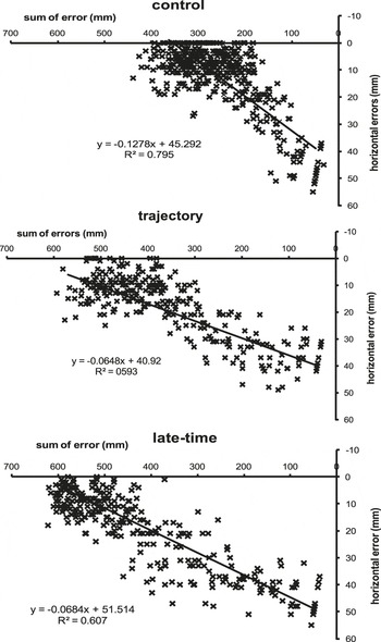
Fig. 5 shows the relation between the error (ordinate) and the cumulative sum of error (abscissa) in block 2. The solid line represents the simple regression line. By using this kind of plot (error-summation scatter gram), Kitazawa et al. (Reference Kitazawa, Kohno and Uka1995) proposed a simple linear parameter model. We can guess uniquely the next error value from the model by using the initial error value and the error correction parameter coefficient (k). The error correction coefficient was calculated from the ratio of the summation error value and the next trial error value. In the control condition, fitting was good, but, in trajectory and late-time conditions, fitting of the regression lines was poor. Kitazawa et al. (Reference Kitazawa, Kohno and Uka1995) indicated that there was linear relation between summation error values and its error (r = 0.9 approximately). However, in our results, in some of adaptation dynamics, we observed poor relation between the error estimate and the observation value by their model. In the scatter diagram of block 2, the values of R 2 for the control, target, on-time, trajectory, and late-time conditions, respectively, were as follows: R 2 = 0.795, 0.710, 0.769, 0.593, and 0.607. The correction coefficients in block 2 were 0.127, 0.118, and 0.094 for the control, target, and on-time conditions, respectively, and were 0.064 and 0.068 for the trajectory and late-time conditions, respectively. The number of errors required for the initial error to be converged was larger in the trajectory and late-time conditions than in the control.
Relation between cumulative sum of error and trial error in three feedback conditions. The solid line represents a simple regression line.

Fitting the dynamics using Kalman filtering
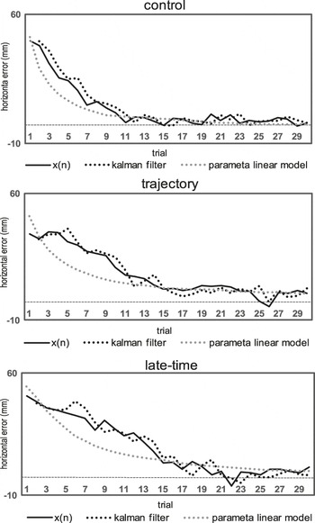
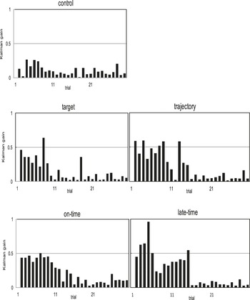
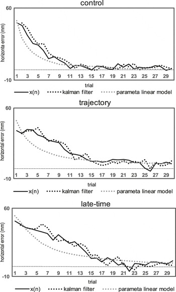
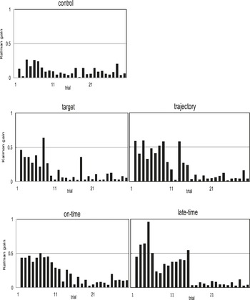
Fig. 6 shows temporal changes in the estimated values obtained using the linear model and Kalman filtering and observed data in the control, trajectory, and late-time conditions. In the control, the estimated values of both models fitted well with the observed values. However, the estimated values obtained using the linear model differed significantly from the observed values in the trajectory and late-time conditions, that is, uncertain state estimation were performed. Parameter estimation using Kalman filtering accurately followed the changes in observed values generated in each trial. The goodness of fit between the estimated and observed values in each model was examined using Akaike information criterion (AIC) (Akaike, Reference Akaike1992) in block 2. AIC would be one way to evaluate two models with different number of parameters. In the control, the value of AIC was 179.0 and 154.0 for the linear model and Kalman filtering, respectively, while these values were 173.6 and 161.1 for the target condition, 202.8 and 159.7 for the trajectory condition, 192.7 and 180.8 for the on-time condition, and 206.9 and 174.0 for the late-time condition. When we estimated optimal model using Kullback–Leibler information, the AIC was the estimator. We can choose the model that a value of the AIC is minimized as an optimal model. Under every condition, the value of AIC of the estimated values for Kalman filtering was smaller than that for the linear model. By examining the variance ratio (Kalman gain) between the prior-estimated and observed values, we can stochastically see that the posterior-estimated value is determined by relying on either the prior-estimated or observed value. In block 2, Kalman gain in the control was 0.07–0.26, whereas in the target and on-time conditions was 0.03–0.50. From eqn. (6), Kalman gain relies on the prior estimation distribution when its value is below 0.5. Kalman gain in the trajectory and late-time conditions was 0.03–0.60 and 0.08–0.95, respectively. Fig. 7 shows the changes in Kalman gain in block 2.
Actual horizontal errors and predicted horizontal errors under three different feedback conditions. The thin line is actual observation value (x(n)), gray dashed line is the estimated values using the parameter linear model, and black dashed line is the predicted values by using the Kalman filter model.
Sequential change of the Kalman gain in block 2 under five different feedback conditions.
Discussion
In 1982, Marr (Marr & Vaina, Reference Marr and Vaina1982) reported that three criteria (computation, representation, and implementation) are required to understand the behavioral characteristics of a biological system. For the computation criterion, he mentioned that naturally occurring phenomena should be simulated using a model based on the computational theory in mathematical engineering. We computationally analyzed the error variance (noise) generated in visuomotor transformation when the visual feedback information was artificially manipulated.
Difference in the magnitude of after effect
The after effect indicates the strength of prism adaptation. The after effects in the trajectory and late-time conditions were smaller than those in the control and target conditions. This means that prism adaptation is affected by the differences in visual feedback conditions. This idea is supported by the results of a prism experiment conducted by Norris et al. (Reference Norris, Greger, Martin and Thach2001), in which the visual feedback was abstracted. They examined changes in after effect under the differences in visual conditions and suggested that interpretations of adaptations made in abstract training and experimental conditions may be greatly affected by visual feedback elements. Welch et al. (Reference Welch, Choe and Heinrich1974) assumed that three internal structures are required for prism adaptation. The first structure is remapping of the visual target position projected on the retina; namely, the mechanism used to recalculate the visual target position on the retina and adapt to that change. The second structure is recalibration of the body’s center to the body’s environment, which is perceived by the motor proprioceptive sensation system. The third structure is a mechanism to shift the visual target position in the head–eye coordinates. We believe that prism adaptation in the trajectory condition is mediated by a recalibration of motor proprioceptive sensation. In the trajectory condition, the apparent trajectory of the fingertip shifted further toward the displacement direction than the predicted trajectory shifts toward the prism-shifted target position. The strategy for prism adaptation in the trajectory condition is postulated to exclude errors between the motor sensation presumed from the predicted trajectory and the sensation generated from the actual fingertip movement. Kitazawa et al. (Reference Kitazawa, Kohno and Uka1995) assumed a forward model that forecast a motor sequence from the predicted trajectory and feed forward to the motor system. The authors thought that motor correction would be accomplished by comparing the real motor sensation with the predicted motor sensation. In the target condition, adaptation was made on the head/eye-centered coordinate system based on the visual feedback error. Wei and Körding (Reference Wei and Körding2009) developed an ideal observer model derived from the specification of a probabilistic generative model. They investigated how motor adaptation was executed in the human reaching with perturbed visual feedback. They assumed that vision and proprioception provide the sensory cues in estimating the hand position, although they are noisy. The visual cue and the proprioceptive cue both reflect the true movement error. They described that new state was estimated based on the movement error occurring from reliable feedback cues. Since the after effect was significantly smaller in the trajectory condition than in the target condition, the degree of prism adaptation was considered to rely on the error in visual sensation rather than the error in motor sensation. These results are different from the study of the grasp movement of Jakobson and Goodale (Reference Jakobson and Goodale1991). They suggested that subjects adopt independent strategies on the basis of the predictability of visual feedback, namely, that at a given kinematic profile of the reaching limbs and visual profile of the object size. However, we thought that the prediction accuracy changed if feedback manipulations were different. Similar to the trajectory condition, the after effect was smaller in the late-time condition than in the control and target conditions. Because convergence characteristics with block 1 were different from control, under conditions of these, visuomotor transformation was insufficiently accomplished regardless of the displacement of the field. The sensory feedback used for adaptation in the late-time condition may not be mundane sensory information. There was a temporal difference in the sensory feedback between the visual profile and kinematic profile. The decrease in after effect of prism adaptation under the late-time condition strongly suggests the necessity of synchronous feedback between the motor sensation and visual position of the fingertip.
Computational model
In the control, target, and on-time conditions, the linear parametric model was successfully able to simulate the dynamics of adaptation. However, in the trajectory and late-time conditions, the goodness of fit to dynamics was low under the linear model rather than the Kalman model. Because the correction rate is constant in the linear model, the predicted parameters based on the sum of errors are uniquely determined. In the case of the trajectory or late-time conditions, where the error variance of trials was large, the linear model could not successfully simulate variation of the external dynamics. A Kalman filtering model expresses hidden variables (parameters) of the state space in the external world using two recurrence eqns. (2) and (3). System noise (ξ) is a system error generated due to unstable sensory calibration processing, and observation noise (ω) is a random error generated due to inadequate visuomotor transformation (Gold & Shadlen, Reference Gold and Shadlen2003; Cisek & Kalaska, Reference Cisek and Kalaska2005; Deneve, Reference Deneve2008). The Kalman filtering model is a sequentially updating model, in which the system error due to the internal model is compared with the random error generated at the visuomotor transformation. We believe that the Kalman filtering model is more suitable for expressing the dynamics of prism adaptation than the linear parametric model. The AIC of the estimated value and observation data in block 2 were smaller in the Kalman filtering model than in the linear parametric model under every condition. Therefore, the predictability of the Kalman filtering model was affirmed.
How is the estimation parameter decided using Kalman filtering?
We infer that the internal dynamics of state-space estimation had changed according to the reliability of visual feedback information (Gold & Shadlen, Reference Gold and Shadlen2001; Tin & Poon, Reference Tin and Poon2005; Burge et al., Reference Burge, Ernst and Banks2008; Izawa & Shadmehr, Reference Izawa and Shadmehr2008; Kiani & Shadlen, Reference Kiani and Shadlen2009; Stevenson et al., Reference Stevenson, Fernandes, Vilares, Wei and Körding2009). A system error variance derived from internal model reflects the accuracy of the estimation parameters. Even if the predicted parameter differs from the visual target position, the prediction accuracy should be high when the system error variance is small. In contrast, when the random error variance is small, the visuomotor transformation is correctly performed. The estimated parameter is updated using Kalman gain. Kalman gain provides the reliability to the difference between an estimated parameter and an observation data. Since Kalman gain in the control and target condition of block 2 was small through all trials, prism adaptation was considered to be generally performed based on the certainty of the estimated parameters. Kalman gain in the trajectory and late-time conditions largely varied with trials. In these conditions, the updated parameter vector should be affected by both the estimated parameter and the actual observation data. When Kalman gain is below 0.5, the estimated parameter derived from the internal system is reliable. When the gain is above 0.5, there is a strong correction based on the observation data. In the late-time condition, there were asynchronous visual feedback input and motor proprioceptive sensation input. Large Kalman gains observed at some trials of late time conditions may indicate that the visual and proprioceptive sensations competed with each other based on the certainty of either information. Consequently, the estimation process was unstably performed. Hence, following that visuomotor transformation was inadequate. Smeets et al. (Reference Smeets, van den Dobbelsteen, de Grave, van Beers and Brenner2006) reported that heterosensory calibration was performed not to accord common coordinates but to select criteria based on the reliability of various sensory information. In the late-time condition, adaptation should be performed, while the reliability of the sensory information was unstable. Therefore, the estimation processing had to be switched at each trial. For actual implementation, the hardware might include multiple system modules that can be instantaneously switched according to the reliability of the sensation (Gold & Shadlen, Reference Gold and Shadlen2001; Kiani & Shadlen, Reference Kiani and Shadlen2009). In this study, we assumed that the estimation dynamics in human was sequentially determined according to the change of the external dynamics. The probabilistic prediction model based on Bayesian estimation could clearly simulate the estimation process even in unstable internal dynamics.
Conclusion
We investigated the dynamics structure of an internal model required for prism adaptation based on the computational model. Consequently, the Kalman filter, a state estimation model based on Bayesian theory, expressed the dynamics of the internal model under uncertain feedback information better than the linear parametric model. We consider that the Kalman filtering is one of the most suitable estimation models for the sequential simulation of dynamics, reaching a level requiring human behavioral decisions.
Acknowledgments
We thank Department of physical therapy of Kansai medical college for equipments setup during the experiments. Conflict of interest: There are no conflicts of interests.