
Introduction
Selective laser melting (SLM) manufactures a three-dimensional (3D) object by adding layer upon layers.[Reference Gan and Wong1] In SLM, a layer of powder is deposited and the laser will scan at the areas marked in the sliced stereolithography file. Once the laser has completed the scanning, a fresh layer of powder will be deposited and the process will repeat until the part is completed. It has seen applications in various industries such as aerospace, automotive as well as medical.[Reference Chua, Wong and Yeong2, Reference Lim, Le, Lu and Wong3] Its freedom of design allows the incorporation of lattice structures to produce lightweight parts.[Reference Yan, Hao, Hussein, Young and Raymont4, Reference Zhou, Shrotriya and Soboyejo5]
SLM is a complex process which involves numerous parameters such as laser power, scanning speed, hatch spacing, layer, and scanning strategy. These parameters contribute to the energy density applied on the powder bed, and will affect the quality of the part.[Reference Fatemi, Ashany, Aghchai and Abolghasemi6–Reference AlMangour, Grzesiak, Borkar and Yang8] Gan and Wong observed that by varying the layer thickness, the porosities and the mechanical properties of the printed parts are affected.[Reference Gan and Wong9] However, it was found that parameters such as the scanning speed and laser power exhibit larger influence over the part's properties.[Reference Yadroitsev, Bertrand and Smurov10]
Relying on experiments to conduct parametric studies can be costly and time-consuming. The use of numerical modeling can assist in determining the optimum sets of processing parameters. Khairallah et al. made use of a numerical model to study the Plateau–Rayleigh instability phenomena on the continuity of the melt track.[Reference Khairallah and Anderson11] Kruth et al. explained the melt pool will tend to reduce its free surface energy. The melt pool can be treated as a half cylinder and when the total surface of the melt pool exceeds that of a sphere with the same volume, it will break to form spheres known as the balling phenomena.[Reference Kruth, Froyen, Van Vaerenbergh, Mercelis, Rombouts and Lauwers12]
Mechanical properties of the printed part can be affected by the melt pool. When a deep keyhole is formed by high energy density, the keyhole will become unstable and collapse, while trapping gas within the melt pool.[Reference Matsunawa, Kim, Seto, Mizutani and Katayama13] This will give rise to porous parts. Kempen et al. observed that fractures are initiated by pores near the surface of the printed part.[Reference Kempen, Thijs, Van Humbeeck and Kruth14] AlMangour et. al. noted that the melt pool affects the hardness and the grain sizes of the printed part.[Reference AlMangour, Grzesiak, Cheng and Ertas15] Another importance of the melt pool is its effect on microstructure evolution. The melt pool can affect the local thermal gradient, which in turn influences the growth rate of the microstructures.[Reference Niendorf, Leuders, Riemer, Richard, Tröster and Schwarze16]
In view of the above, this paper looks at how different processing parameters will affect the melt pool and track formation. These investigations will reveal the relationships between the different characteristics of the melt pool, which in turn will affect the mechanical properties of the printed part.
Methodology
To numerically generate the powder bed, a Discrete Element Method model using LIGGGHTS® software was carried out.[17] The powder size follows a Gaussian distribution of mean diameter 27 µm with a full width at half maximum value of 5 µm. The powders were released from a height of 700 µm onto a 1000 × 200 × 200 µm substrate to simulate the random scattering of powders observed in the actual experiment. The coordinates and the radii of individual powders are extracted and input into a CFD software (OpenFOAM®) which is capable of modeling the melting and solidification process.
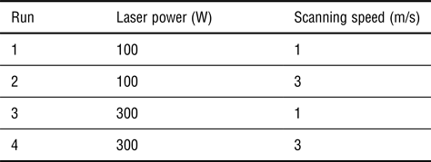
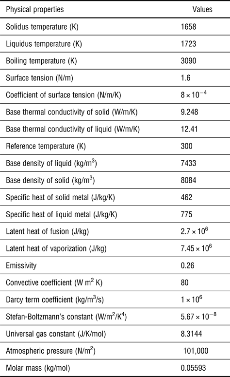
OpenFOAM® (Open Field Operation and Manipulation) is an open-source Computational Fluid Dynamics toolbox which is used in the present study to model the SLM process.[18] The metal used in the simulation is SS316L. The mesh size used in the simulations was 2.5 µm. The parameters used for the single-track model for different runs are shown in Table I. Table II shows the physical properties of SS316L and the constants used for the modeling. In the model, a timestep of 10 ns were used. The length of each track was 800 µm. The data from each simulation were extracted and plotted against each other for comparisons.
Parameters used

Physical properties of SS316L and constants used in the simulations.

Thermal fluids equations
There are two different phases in the model, metallic and gas phase. The volume of fluid method was used to distinguish between the metallic and gas phases.[Reference Qiu, Panwisawas, Ward, Basoalto, Brooks and Attallah19] The phase fraction, α, is used to distinguish the different phases present in the simulation. The relationship is given as
 $$\alpha _1 + \alpha _2 = 1$$
where the metallic phase is represented by α1 and the gas phase is represented by α2.
In the metallic phase, the metal can exist in the solid or liquid state. To determine the state of the metal, a liquid fraction, γ was introduced.[Reference Rösler and Brüggemann20] The values of γ lies between 0 and 1. When γ = 0, the metal is in the solid state. When γ = 1 the metal is in the liquid state. Any values between 0 and 1 will be referred as the mushy state.
In the simulation, there will be meshes which comprise air and metal mixture. In this region, the average material property,  $\bar \varphi $, is used and is calculated using
 $$\bar \varphi = \varphi _{{\rm air}}\cdot \alpha _2 + \varphi _{{\rm metal}}\cdot \alpha _1$$
where φ air is the material property for air and φ metal is the material of the metal. An example of the volume average of the density is given by  $\bar \rho = \rho _{{\rm air}}\cdot {\rm \alpha} _2 + \rho _{{\rm metal}}\cdot {\rm \alpha} _1$.
There are three main governing equations used in the model. They are the conservation of mass, conservation of momentum, and conservation of energy equations. The metal was assumed to be incompressible and therefore the continuity equation can be represented by
 $$\nabla \cdot {\bi \vec u} = 0$$
where  ${\bi \vec u}$ is flow velocity.
For the conservation of momentum, the forces acting on the system are considered. The recoil pressure, Marangoni force, buoyancy force, surface tension, and gravitational force can be found on the right-hand side of[Reference Panwisawas, Qiu, Anderson, Sovani, Turner, Attallah, Brooks and Basoalto21]
 $$\eqalign{\displaystyle{{\partial \bar \rho {\bi \vec u}} \over {\partial t}} & + \nabla \cdot \lpar {\bar \rho {\bi \vec u} \otimes {\bi \vec u}} \rpar = - \nabla p \cr & + \nabla \cdot \lpar {\bar \mu \cdot \nabla {\bi \vec u}} \rpar + \bar \rho g\hat e_z\beta \lpar {T - T_{{\rm ref}}} \rpar - K_c\left[ {\displaystyle{{{\lpar {1 - \gamma} \rpar }^2} \over {\gamma^3 + C_k}}} \right]{\bi \vec u} \cr &+ \left\{ {\sigma k\hat n + \displaystyle{{d\sigma} \over {dt}}\lsqb {\nabla T - \hat n\lpar {\hat n\cdot \nabla T} \rpar } \rsqb + p_v} \right\}\vert {\nabla \alpha_1} \vert \displaystyle{{2\bar \rho} \over {\lpar {\rho_{{\rm metal}} + \rho_{{\rm air}}} \rpar}}}$$
where  $\bar \rho $ is the volume average of density,
 $\bar \mu $ is the volume average of viscosity, t is the time, T is the temperature, T ref is the reference temperature, p is pressure, g is gravitational acceleration, and p v is the recoil pressure.
 ${\hat e}_z$ is the unit normal to the gravitational force, β is the thermal expansion coefficient, and K c is the permeability coefficient. C k is a constant to avoid division by zero, σ is the surface tension, and k is the surface curve normal to
 $\hat n$.
 $\; \vert {\nabla {\rm \alpha}_1} \vert $ was used to transform a surface force per unit area into a volumetric surface force.[Reference Saldi22, Reference Brackbill, Kothe and Zemach23]
The Marangoni force is expressed as  $(d\sigma /dt)\lsqb {\nabla T - \hat n\lpar {\hat n\cdot \nabla T} \rpar } \rsqb $. From the equation, it shows that the force is temperature dependent. In the melt pool, the temperature gradient will result in a difference in surface tension.[Reference DebRoy and David24] The molten metal will flow from the region with low surface tension to a region with high surface tension.
During the laser melting process, the surface of the molten metal may reach over the boiling point of the metal. The metal will vaporize and exerts a downward pressure on the melt pool, commonly observed as the keyhole phenomena. This pressure is known as the recoil pressure and is defined by[Reference Cho, Farson, Milewski and Hollis25]
 $$p_v = 0.54p_0{\rm \; exp}\left( {\Delta H_V\cdot M\displaystyle{{T - T_{LV}} \over {RTT_{LV}}}} \right)$$
where p 0 is the atmospheric pressure, ΔH V is the enthalpy change due to vaporization, M is the molar mass of the metal, T LV is the evaporation temperature of the metal, and R is the universal gas constant.
In the model, the heat transfer due to conduction, convection, radiation, laser input, and phase transformation are represented in the conservation of energy equation, given by
 $$\eqalign{& \displaystyle{{\partial {\bar C}_p\bar \rho T} \over {\partial t}} + \nabla \cdot \lpar {{\bi \vec u}{\bar C}_p\bar \rho T} \rpar = - \displaystyle{{\partial \bar \rho \Delta H_f} \over {\partial t}} - \nabla \cdot \lpar {\bar \rho {\bi \vec u}\Delta H_f} \rpar + \cr & {\nabla \cdot \lpar {\bar k\nabla T} \rpar + Q_T - \lsqb {h_c\lpar {T - T_{{\rm ref}}} \rpar }} \cr & + \sigma_s\varepsilon \lpar {T^4 - T_{{\rm ref}}^4} \rpar + Q_v \rsqb \vert {\nabla \alpha_1} \vert \displaystyle{{2{\bar C}_p\cdot \bar \rho} \over {\lpar {C_{\,p\lpar {{\rm metal}} \rpar }\cdot \rho_{{\rm metal}} + C_{p\lpar {{\rm air}} \rpar }\cdot \rho_{{\rm air}}} \rpar }}}$$
where Q T is the laser input, ΔH f is the enthalpy change due to fusion,  $\bar k$ is the volume average of thermal conductivity, h c is the heat transfer coefficient,
 $\bar C_p$ is the volume average of specific heat, σ s is the Stefan–Boltzmann constant, ε is the emissivity, Q v is the heat loss due to evaporation. The term
 $ - (\partial \bar \rho {\rm \Delta} H_f/\partial t) - \nabla \cdot \lpar {\bar \rho {\bi \vec u}{\rm \Delta} H_f} \rpar $ is the enthalpy change due to the melting of the metallic phase. The conduction, convection, and radiation are given by
 $\nabla \cdot \lpar {\bar k\nabla T} \rpar $, h c(T − T ref), and
 $\sigma _s\varepsilon \lpar {T^4 - T_{{\rm ref}}^4} \rpar $, respectively.
The laser beam intensity can be approximated as a Gaussian distribution given by
 $$I = \displaystyle{{2\eta P} \over {\pi r^2}}\hbox{exp}\left[ { - 2\displaystyle{{{\lpar {x + v\cdot t - x_0} \rpar }^2 + {\lpar {y - y_0} \rpar }^2} \over {r^2}}} \right]$$
where η is the absorptivity coefficient, p is the laser power, x and y are the coordinates of the center of the laser beam at time t, x 0, and y 0 are the starting coordinates of the laser beam, r is the radius of the laser beam, and v is the scanning speed. The radius of the laser beam for the simulation is set to be 27 µm and the absorptivity was taken to be 0.4.
To obtain the laser beam energy density, the intensity of the beam can be approximated as
 $$Q_T = \displaystyle{{I\cdot f_{{\rm absorb}}} \over {\Delta z}} $$
where Δz represents the height of the numerical grid and f absorb is an indicator ranging from 0 to 1 to ensure the heat flux is only applied on the top surface of the metal. Further explanation of f absorb can be found in the supplementary material. In this model, the Fresnel absorption was neglected due to the high computational cost.
In the laser process, the prominence of evaporation increases along with temperature increase and cannot be neglected. Therefore, the heat loss due to evaporation is defined as[Reference Cho, Farson, Milewski and Hollis25]
 $$Q_v = 0.82\displaystyle{{\Delta H_v\cdot M} \over {{\lpar {2\pi MRT} \rpar }^{0.5}}}p_0\hbox{exp}\left( {\Delta H_v\cdot M\displaystyle{{T - T_{LV}} \over {RTT_{LV}}}} \right) $$
Results and discussions
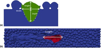
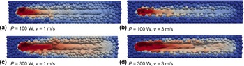
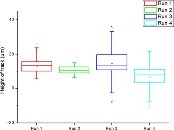
Figure 1 illustrates how the measurements of the dimensions were taken for Table II. Figure 1(a) shows the cross-section of a solidified track (green region) when measuring the height, width, and depth of the melt pool. Fig. 1(b) shows the red region representing the molten metal to record the reading of the length of the melt pool. Figure 2 shows the top view of the melt tracks. The dimensions of the melt pool are shown in Table III. Comparing Figs. 2(a) and 2(c) to Figs 2(b) and 2(d) respectively, it can be observed that increasing the scanning speed from 1 m/s to 3 m/s will induce narrower tracks. Since the melt pool generated from a higher scanning speed is smaller than that of a lower scanning speed, it will affect the width of the melt track. With a narrower track width, the hatch spacing will have to be reduced to avoid unmelted regions between tracks. From the energy density equation,[Reference Yap, Chua and Dong26] it can be noted that despite run 1 and run 4 sharing the same energy density, their melt track profiles vary significantly with run 4 having a wider melt pool. Therefore, it shows that the parameters have different impacts on the melt pool. This is in agreement with the experimental observation by Bertoli et al.[Reference Scipioni Bertoli, Wolfer, Matthews, Delplanque and Schoenung27] In their experiments, the track with a lower laser power and scanning speed displayed a more consistent melt profile. Similarly from this model, Fig. 2(a) has a smoother melt surface when compared with Fig. 2(d). In Fig. 3, the heights of the tracks were measured and plotted to show the mean and deviations which relate to the surface roughness of the track. A greater deviation would directly translate to a rougher surface of the track. The difference in surface roughness can be explained using Rayleigh–Plateau instability principle. It occurs due to the effect of surface tension. The melt pool can be observed as a semi-cylindrical fluid. When the length to width ratio of the melt pool increases beyond a critical value of 2.1, it will result in Raleigh–Plateau instability.[Reference Kruth, Froyen, Van Vaerenbergh, Mercelis, Rombouts and Lauwers12, Reference Rombouts, Kruth, Froyen and Mercelis28] If the melt pool is long, it will result in necking and breaking of the semi-cylindrical shape, resulting in unevenness of the melt pool profile. In Table III, the lengths of the melt pool were measured. Comparing the length of the melt pools to the surface roughness, a positive correlation can be established.
Measurements of the melt pool's dimension on the 1000 × 200 × 200 µm substrate model. (a) Green represents the solidified track and (b) red region represents the molten metal.

Top view of the tracks of (a) run 1, (b) run 2, (c) run 3, and (d) run 4.

Heights of tracks along the scanning direction.

Dimensions of melt pools

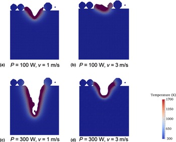
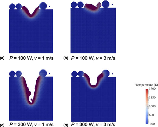
Figure 4 shows the cross-section of the melt pool during the melting process. Comparing Figs. 4(a) and 4(c), it was observed that the laser power primarily affects the depth of the melt pool. The widths of run 1 and 3 are approximately similar, while their depths differ significantly. Taking Run 2 as an example, increasing the laser power to 300 W will achieve a greater impact on the resultant depth than reducing the scanning speed to 1 m/s. In run 1, the low scanning speed will result in heat being conducted away from the melt pool. Temperature around the melt pool will be lowered leading to a reduction in the vaporization of the molten metal. This will lead to a decrease in recoil pressure and giving a shallower depth. In run 4, the high laser power will be absorbed by the metal, resulting in its temperature soaring above the boiling point. The higher rate of metal vaporizing will increase the recoil pressure and therefore, leading to a deeper depth. When comparing the effects of laser power and scanning speed on the width of the track, varying the laser power from 100 W to 300 W will give a wider melt pool than using a lower scanning speed of 1 m/s. A similar conclusion can be drawn from experimental results.[Reference Yadroitsev, Yadroitsava, Bertrand and Smurov29]
Cross-sections of melt pool of (a) run 1, (b) run 2, (c) run 3, and (d) run 4.

Conclusions
In this paper, the use of simulation is able to show the relationship between the length of the melt pool with the resultant surface roughness of the track. A longer melt pool will give rise to a rougher surface due to the instability of the melt pool.
Next, it can be concluded that laser power has more effect over the width and depth of the melt pool. Similar conclusions can be derived from experimental studies by Yadroitsev et al.[Reference Yadroitsev, Yadroitsava, Bertrand and Smurov29] This shows that modeling of SLM process can aid in the parametric study of SLM and provide a good representation of the experiments. It can help to reduce the time and materials cost of conducting experiments.
Supplementary Material
The supplementary material for this article can be found at https://doi.org/10.1557/mrc.2018.180
Acknowledgements
The work is funded by SLM Solutions Group AG (RCA-14/089) in collaboration with Singapore Centre for 3D Printing, Nanyang Technological University, Singapore. The work is also supported by EDB-IPP and SLM Solutions Singapore Pte Ltd.
Conflict of interest
The authors declare no conflict of interest.