A. Institutional Background

Although risk preferences are central to decisions under uncertainty and economic analysis, measuring risk aversion has been challenging. In recent years, eliciting risk aversion parameters from insurance data has received increasing attention (Cohen and Einav (Reference Cohen and Einav2007), Sydnor (Reference Sydnor2010), Barseghyan, Prince, and Teitelbaum (Reference Barseghyan, Prince and Teitelbaum2011), Einav, Finkelstein, Pascu, and Cullen (Reference Einav, Finkelstein, Pascu and Cullen2012), Barseghyan, Molinari, O’Donoghue, and Teitelbaum (Reference Barseghyan, Molinari, O’Donoghue and Teitelbaum2013)). In this article, we follow Cohen and Einav (Reference Cohen and Einav2007) to estimate individuals’ levels of risk aversion by exploiting data on deductible choices in auto insurance contracts. The key assumption of using insurance data to estimate individuals’ risk aversion is that individuals choose insurance contracts to hedge against risk.

Our main data source is the auto insurance platform of CIITC, which constructs and operates a centralized platform for sharing insurance data and information in China. The platform is publicly accessible and pools nationwide insurance data and information for motor vehicles in China.

In China, motor vehicles are mandatorily insured with “Automobile Mandatory Insurance” and optionally insured with motor vehicle commercial insurance, from which we can observe individuals’ deductible choices. Commercial insurance includes primary insurance and optional insurance. Primary insurance covers loss insurance, Automobile Third-Party Liability insurance, onboard personnel liability insurance, and theft insurance. For primary insurance, the default deductible rate is 15%. For optional insurance, individuals can choose a policy with a zero-deductible rate. The deductible amount for the insurer of each policy equals the coverage multiplied by the loss rate multiplied by the deductible rate of the policy, in which the loss rate equals the ratio of realized loss to the coverage. Unlike the typical options of a regular deductible and a low deductible in Israel, for instance, individuals in China have the option to choose a policy with a zero-deductible rate and an additional premium or a policy with a 15% deductible rate and no additional premium. All else equal, individuals who choose the policy with a lower deductible rate despite the additional premium are more likely to exhibit higher risk aversion. The mandatory policy, the primary insurance structure, and the observable variation in deductible choices make the screening model of risk preferences plausible.

B. Benchmark Model of Deductible Choice

Let $ p $ , $ d $ , $ I $ , $ t $ denote the premium rate, the deductible rate, the coverage, and the duration of each additional policy, respectively. Consider the two deductible choices: ( $ {p}_i^0 $ , $ {d}_i^0 $ ) stands for the low deductible choice, where individual $ i $ needs to pay an additional premium $ {I}_i\times {p}_i^0 $ and the deductible rate $ {d}_i^0 $ is 0; and ( $ {p}_i^1 $ , $ {d}_i^1 $ ) stands for the high deductible choice, where individual $ i $ does not need to pay an additional premium $ \left({p}_i^1=0\right) $ and the deductible rate $ {d}_i^1 $ is fixed at 15%. The loss rate of each claim is $ L $ , which is the ratio of realized loss to the coverage and is assumed to be lognormally distributed. Consistent with the key assumption in Cohen and Einav (Reference Cohen and Einav2007), the annual claim rate of individual $ i $ , $ {\lambda}_i $ , is assumed to follow a Poisson process and to be known to individual $ i $ . In addition, there is no moral hazard in the model, so that $ {\lambda}_i $ is independent of the deductible choice.Footnote ¹ Therefore, by definition, a risk-neutral individual $ i $ would choose the low deductible choice if and only if the claim rate $ {\lambda}_i\ge \frac{\left({p}_i^0-{p}_i^1\right)\times {I}_i}{\left({d}_i^1-{d}_i^0\right)\times {I}_i\times L}=\frac{p_i^0}{d_i^1\times L}. $

For individual $ i $ with endowment wealth of $ {w}_i $ , the expected utility of a deductible choice $ \left({p}_i,{d}_i\right) $ can be written as

(1) $$ v\left({p}_i,{d}_i\right)=\left(1-{\lambda}_i{t}_i\right)u\left({w}_i-{I}_i{p}_i{t}_i\right)+{\lambda}_i{t}_iu\left({w}_i-{I}_i{p}_i{t}_i-{I}_i{Ld}_i\right), $$

where $ u(w) $ is the utility function.

To estimate individuals’ levels of risk aversion, the basic idea is that, when the expected utility is indifferent between the low deductible choice and the high deductible choice, it will provide a lower bound on the risk aversion of individuals who choose the low deductible choice and an upper bound on the risk aversion of individuals who choose the high deductible choice. Therefore, we can analyze the equation $ v\left({p}_i^0,{d}_i^0\right)=v\left({p}_i^1,{d}_i^1\right) $ and proceed to calculate the expression of the claim rate as

(2) $$ {\displaystyle \begin{array}{c}\lambda =\underset{\hskip0.22em {t}_i\to 0\;\hskip0.1em }{\mathit{\lim}}\frac{\frac{1}{t_i}\left(u\left({w}_i-{I}_i{p}_i^0{t}_i\right)-u\left({w}_i-{I}_i{p}_i^1{t}_i\right)\right)}{u\left({w}_i-{I}_i{p}_i^1{t}_i-{I}_i{Ld}_i^1\right)-u\left({w}_i-{I}_i{p}_i^0{t}_i-{I}_i{Ld}_i^0\right)-u\left({w}_i-{I}_i{p}_i^1{t}_i\right)+u\left({w}_i-{I}_i{p}_i^0{t}_i\right)}\\ {}=\frac{\left({p}_i^0-{p}_i^1\right){I}_i{u}^{\prime}\left({w}_i\right)}{u\left({w}_i-{I}_i{Ld}_i^0\right)-u\left({w}_i-{I}_i{Ld}_i^1\right)}.\end{array}} $$

Using Taylor’s expansion, we have

(3) $$ u\left(w-\epsilon \right)=u(w)-{u}^{\prime }(w)\epsilon +\frac{1}{2}{u^{\prime}}^{\prime }(w){\epsilon}^2+o\left({\epsilon}^2\right). $$

Combining equations (2) and (3) and using the definition of absolute risk aversion, we can infer the individual’s level of absolute risk aversion as

(4) $$ r\equiv \frac{-{u^{\prime}}^{\prime }(w)}{u^{\prime }(w)}=\frac{\frac{p_i^0-{p}_i^1}{\lambda \left({d}_i^1-{d}_i^0\right)}-E(L)}{\frac{d_i^0+{d}_i^1}{2}{I}_iE\left({L}^2\right)}, $$

where $ r $ stands for the individual’s absolute risk aversion, and $ E(L) $ and $ E\left({L}^2\right) $ are the first and second moments of the loss rate, respectively.

C. Estimating Absolute Risk Aversion

Based on individuals’ deductible choices in the auto insurance data, $ \left({p}_i,{d}_i\right) $ and $ {I}_i $ are observable. In particular, $ {d}_i^0=0 $ , $ {d}_i^1=0.15 $ , and $ {p}_i^1=0 $ . We can therefore rewrite the formula for absolute risk aversion in equation (4) as

(5) $$ r=\frac{\frac{p_i^0}{0.15\times \lambda }-E(L)}{0.075\times {I}_iE\left({L}^2\right)}. $$

In addition, we can estimate the mean and variance of the loss rate from the realized insurance claim data. For example, we randomly select about 10,000 claims; the fitted loss rate distribution is plotted in Supplementary Material Figure IA.I. The loss rate of claims is approximately lognormally distributed, as is typically assumed in the literature. In our sample data set, the mean and variance of the loss rate are 0.02 and 0.00285, respectively.

In an econometric exercise, we use the observable data, denoted by $ {x}_i $ , from the deductible choices to estimate the annual claim rate and the absolute risk aversion of each individual $ i $ : $ \left({\lambda}_i,{r}_i\right) $ . Assuming that $ \left({\lambda}_i,{r}_i\right) $ is bivariate lognormally distributed, we can write the econometric model as

(6) $$ \mathit{\ln}\left({\lambda}_i\right)={x}_i^{\prime}\beta +{\epsilon}_i, $$

(7) $$ \mathit{\ln}\left({r}_i\right)={x}_i^{\prime}\gamma +{\delta}_i, $$

and the residuals $ {\epsilon}_i $ and $ {\delta}_i $ satisfy

(8) $$ \left(\begin{array}{c}{\epsilon}_i\\ {}{\delta}_i\end{array}\right)\sim N\left(\begin{array}{c}\left[\begin{array}{c}0\\ {}0\end{array}\right],\left[\begin{array}{cc}{\sigma}_{\lambda}^2& {\rho \sigma}_{\lambda }{\sigma}_r\\ {}{\rho \sigma}_{\lambda }{\sigma}_r& {\sigma}_r^2\end{array}\right]\end{array}\right). $$

The variable $ {\lambda}_i $ in equation (6) and the variable $ {r}_i $ in equation (7) are treated as latent variables, since they are unobservable. We observe the realized number of claims and the deductible choices of individuals on the auto insurance platform. As is typically assumed, the number of claims of individual $ i $ is generated by a Poisson process:

(9) $$ {Claims}_i\sim Poisson\left({\lambda}_i{t}_i\right). $$

In addition, individual $ i $ chooses the low deductible choice $ \left({Choice}_i=0\right) $ 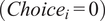if and only if the risk aversion $ {r}_i $ is higher than the lower bound generated from the formula in equation (5) when $ \lambda ={\lambda}_i $ :

(10) $$ \begin{array}{l}\mathit{\Pr}\left({Choice}_i=0\right)=\mathit{\Pr}\left(\begin{array}{c}{r}_i>\frac{\frac{p_i^0}{0.15\times {\lambda}_i}-E(L)}{0.075\times {I}_iE\left({L}^2\right)}\end{array}\right)\\ {}\hskip2.4em =\mathit{\Pr}\left(\begin{array}{c}{e}^{x_i^{\prime}\gamma +{\delta}_i}>\frac{\frac{p_i^0}{0.15\times {e}^{x_i^{\prime}\beta +{\epsilon}_i}}-E(L)}{0.075\times {I}_iE\left({L}^2\right)}\end{array}\right).\end{array} $$

Based on the assumption in equation (9) and the result in equation (10), we can estimate the parameters $ \beta $ and $ \gamma $ from the auto insurance data and then recover $ {\lambda}_i $ and $ {r}_i $ . In practice, we use the Markov chain Monte Carlo (MCMC) algorithm, specifically Gibbs sampling, to obtain the limiting distribution and then the posterior distribution of claims and choices. Finally, we obtain the estimated annual claim rate and the absolute risk aversion of each individual after 100,000 iterations. See the Supplementary Material in Cohen and Einav (Reference Cohen and Einav2007) for details on the MCMC algorithm.

A. Insurance Data

The original sample from the auto insurance platform of CIITC comprises 10 million policy-level records from 2011 to 2017, including all first-time and repeated applications. The sample was randomly drawn from the nearly 200 million policy-level records in the entire platform at the individual level: once an individual is selected into the sample, all of that individual’s policies across the entire sample period are included.Footnote ² This design ensures that we observe the complete insurance history for each sampled individual, which is essential for exploiting within-person variation and including person fixed effects. For each record, the data contain demographic characteristics of the applicant, car attributes, insurance clauses, and claims within the duration of the policy. Supplementary Material IA.1 reports a description of the full detailed sample.

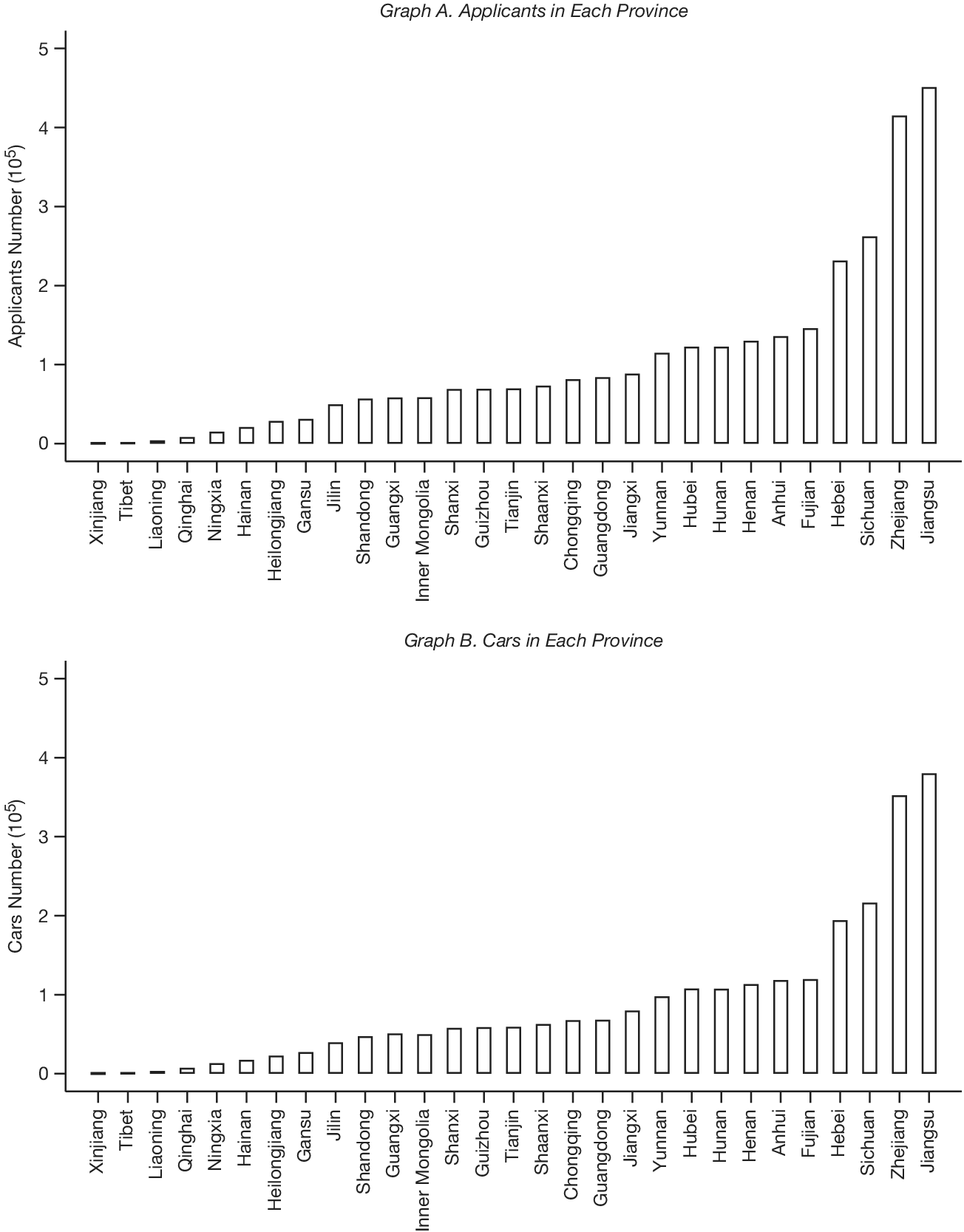
In this sample, auto insurance applications are aggregated on a quarterly basis for each applicant.Footnote ³ There are 2,951,145 unique applicants with 10,229,255 valid observations in the final sample and nearly 101,764 applicants on average in each province. The distributions of the final sample in each province are reported in Figure 1. Jiangsu and Zhejiang have the most applicants, while Xinjiang and Tibet have the least. In addition, we collect the province-level and city-level macro outputs and consumption data, lottery sales data, stock trading volume, bond trading volume, and the total trading volume of capital assets from the Wind database.

FIGURE 1Sample Distributions by Province

Figure 1 shows the sample distribution across provinces. Graph A reports the number of applicants; Graph B reports the number of cars. There are 29 provinces in the sample. The final sample is a 5% random draw from the original China Insurance Information Technology Management (CIITC) sample.

FIGURE 1 Long description

Two vertically stacked bar charts.

Top panel: Graph A. Applicants in Each Province. The y-axis is labeled Applicants Number 10 super 5, with a scale from 0 to 5. The x-axis lists 29 provinces. From left to right, the bars show a steady increase starting near zero for Xinjiang, Tibet, and Liaoning. The values rise gradually through central provinces like Shanxi and Hubei, then increase sharply at the right end. The highest counts are in Hebei, Sichuan, Zhejiang, and Jiangsu, with Jiangsu reaching approximately 4.5 times 10 super 5.

Bottom panel: Graph B. Cars in Each Province. The y-axis is labeled Cars Number 10 super 5, with a scale from 0 to 5. The x-axis lists the same 29 provinces in the same order as Graph A. The data distribution mirrors Graph A, showing a low concentration in western provinces and a high concentration in eastern coastal provinces. Jiangsu again represents the peak at approximately 3.8 times 10 super 5.

Provinces listed on the x-axis for both graphs are: Xinjiang, Tibet, Liaoning, Qinghai, Ningxia, Hainan, Heilongjiang, Gansu, Jilin, Shandong, Guangxi, Inner Mongolia, Shanxi, Guizhou, Tianjin, Shaanxi, Chongqing, Guangdong, Jiangxi, Yunnan, Hubei, Hunan, Henan, Anhui, Fujian, Hebei, Sichuan, Zhejiang, and Jiangsu.

B. Summary Statistics

Summary statistics for the main variables are given in Table 1. The final sample includes 10,229,255 applicant-quarter observations, referring to applications of 2,951,145 individuals. The applicants’ absolute risk aversion (ARA)—estimated using the approach described in Section II—has an average of $ 6.842\times {10}^{-4} $ $ {CNY}^{-1} $ . It is about four times the estimate of $ 1.02\times {10}^{-3} $ $ {USD}^{-1} $ in Cohen and Einav (Reference Cohen and Einav2007) for auto insurance applicants and about 14 times the estimate $ 3.1\times {10}^{-4} $ $ {USD}^{-1} $ in Gertner (Reference Gertner1993) for television game show participants. Since the exchange rate of the USD to the Chinese CNY is between 6 and 7 from 2011 to 2017, our estimates are largely consistent with the literature.

TABLE 1Summary Statistics

TABLE 1 Long description

The table contains 9 columns: Variable, N, Mean, Std. Dev., p1, p25, Median, p75, and p99.

* A R A times 10 super minus 4: N 10,229,255; Mean 6.842; Std. Dev. 9.141; Median 3.748.

* Ln A R A: N 10,229,255; Mean minus 8.259; Std. Dev. 2.297; Median minus 7.889.

* R R A: N 8,997,276; Mean 15.112; Std. Dev. 22.116; Median 7.818.

* Ln R R A: N 8,997,276; Mean 1.686; Std. Dev. 2.334; Median 2.056.

* Male: N 10,229,255; Mean 0.723; Std. Dev. 0.447; Median 1.

* Age: N 10,229,255; Mean 38.292; Std. Dev. 9.289; Median 38.

* LnExpense: N 10,229,255; Mean 7.225; Std. Dev. 0.479; Median 7.178.

* LnCoverage: N 10,229,255; Mean 11.452; Std. Dev. 0.584; Median 11.449.

* CarAge: N 10,229,255; Mean 2.914; Std. Dev. 2.412; Median 2.

* G D P Growth: N 10,229,255; Mean 0.087; Std. Dev. 0.018; Median 0.083.

* IndGrowth: N 9,649,944; Mean 0.090; Std. Dev. 0.036; Median 0.083.

* RetailGrowth: N 9,649,944; Mean 0.119; Std. Dev. 0.024; Median 0.119.

* R Estate Growth: N 9,646,529; Mean 0.124; Std. Dev. 0.116; Median 0.110.

* ConsGrowth: N 9,649,944; Mean 0.084; Std. Dev. 0.036; Median 0.079.

We follow the standard risk aversion model to estimate the RRA of applicants by multiplying the ARA by the annual consumption. Since annual consumption data of applicants are unavailable, we instead use per capita annual consumption of the city in which the applicant lives. There are 8,997,276 observations of estimated RRA. The missing observations are due to the unavailability of consumption data in certain cities. The estimated RRA has an average value of 15.112 and a median value of 7.818, with a standard deviation of 22.116, which is also of the same order of magnitude as the estimate of 14.84 in Cohen and Einav (Reference Cohen and Einav2007) and 4.79 in Gertner (Reference Gertner1993).

In addition to the risk aversion measures, the applicants in our sample are between 22 and 62 years old, with an average age of 38.3 years, and 72.3% of the applications are from male applicants. For the loss policies, the averages of the natural logarithms of premium and coverage are 7.225 and 11.452. The insured cars have been used for 2.914 years on average. The real quarterly GDP growth rate of provinces in our sample has an average of 8.7% with a standard deviation of 1.8%. As alternative macroeconomic indicators, the mean of the real quarterly growth rates of industrial production, aggregate retail sales, and real estate investment in each province are 9.0%, 11.9%, and 12.4%, respectively. Per capita consumption has an annual growth rate of 8.4% with a standard deviation of 3.6%.

C. Validity of Risk Aversion Estimates

Although risk aversion has long been discussed in theoretical studies, quantitatively measuring individuals’ risk aversion is not easy. A body of empirical studies measures risk preferences using hypothetical survey questions, such as Dohmen, Falk, Huffman, Sunde, Schupp, and Wagner (Reference Dohmen, Falk, Huffman, Sunde, Schupp and Wagner2011), Barsky, Juster, Kimball, and Shapiro (Reference Barsky, Juster, Kimball and Shapiro1997), and Guiso et al. (Reference Guiso, Sapienza and Zingales2018), or by television game show participation, such as Gertner (Reference Gertner1993).

In this article, we follow Cohen and Einav (Reference Cohen and Einav2007) to estimate individuals’ levels of risk aversion based on their deductible choices in auto insurance, from which we can study both the time-series and cross-sectional variations in risk aversion. As discussed in Section II, our estimated ARA and RRA are of the same order of magnitude as those estimates in the literature. We now further examine the validity of our estimated risk aversion from several angles.

First, we estimate panel regressions to test whether the estimated risk aversion is correlated with individuals’ demographic characteristics. The results are reported in Table 2. We estimate panel regressions with no fixed effects or with year $ \times $ quarter fixed effects, with the dependent variable being the ARA measure, as reported in columns 1 and 2, the logarithm of the ARA measure, as reported in columns 3 and 4, the RRA measure, as reported in columns 5 and 6, or the logarithm of the RRA measure, as reported in columns 7 and 8. In the Chinese auto insurance market, we do not find significant evidence supporting the inference that females are more risk averse than males. In the level regressions (columns 1–2 and 5–6), male applicants even exhibit significantly higher absolute and RRA. However, in the logarithm specifications (columns 3–4 and 7–8), the male coefficients are economically small and statistically indistinguishable from 0, indicating that male and female applicants do not differ significantly in risk aversion. The estimated coefficients of age show an increasing pattern of individuals’ risk aversion over the life cycle: individuals become more risk averse as they grow older. These findings together indicate that applicants’ risk aversion increases with age.

TABLE 2Regressions of Risk Aversion on Demographic Characteristics

TABLE 2 Long description

The table presents panel regressions with eight columns. The dependent variables are A R A (Columns 1 and 2), Ln open parenthesis A R A close parenthesis (Columns 3 and 4), R R A (Columns 5 and 6), and Ln open parenthesis R R A close parenthesis (Columns 7 and 8).

Independent variables and their coefficients (with t-statistics in parentheses) include:

* Male: Positive and significant for A R A (0.384 and 0.394) and R R A (0.713 and 0.790), but insignificant for logarithm forms.

* Age: Consistently positive and significant across all models, ranging from 0.011 to 0.208.

* LnExpense: Consistently positive and highly significant across all models, with coefficients ranging from 0.520 to 17.275.

* LnCoverage: Consistently negative and highly significant across all models, with coefficients ranging from -1.924 to -38.480.

* CarAge: Mixed results; negative and significant in logarithm models and Column 2, but positive and significant in Column 5 and 6.

* Constant: Positive and highly significant in all specifications.

Bottom rows specify:

* Fixed effect: ‘No’ for odd-numbered columns; ‘Year times quarter’ for even-numbered columns.

* Number of Observations: 10,229,255 for A R A models; 8,997,276 for R R A models.

* Within R-squared: Ranges from 0.240 to 0.635.

We then investigate the correlation of our risk aversion measure with other risky asset preferences. A classic way to estimate individuals’ risk aversion in the literature is to measure their preference for lottery choices, such as Donkers, Melenberg, and Van Soest (Reference Donkers, Melenberg and Van Soest2001), Holt and Laury (Reference Holt and Laury2002), and Andersen, Harrison, Lau, and Rutström (Reference Andersen, Harrison, Lau and Rutström2008). In another study, Guiso et al. (Reference Guiso, Sapienza and Zingales2018) use the subjective choices of respondents on lotteries as the quantitative indicator of their risk preferences. To validate our measure of risk aversion, we examine the correlation of our risk aversion measure with lottery sales growth. In each province, we average the risk aversion measure of applicants as the aggregate indicator of the province on a quarterly basis. We estimate the panel regression of the quarterly growth rate of lottery sales, which is calculated as the change in the natural logarithm of current lottery sales to the 4-quarter-prior lottery sales within the province, on the aggregate risk aversion indicator in the province-quarter panel. We use the change in the natural logarithm of aggregate lottery sales as the dependent variable to mitigate the influence of autocorrelation. The results are reported in Table 3. In columns 1 and 2 of Panel B, the growth rate of lottery sales is negatively correlated with the aggregate ARA of individuals. The estimated coefficient of $ Ln(ARA) $ is −0.169, which is statistically significant with a $ t $ -statistic of −4.61. The RRA indicator $ Ln(RRA) $ has an estimated coefficient of −0.140 with a $ t $ -statistic of −5.26, remaining statistically significant. The aforementioned results remain unchanged when we replace the explanatory variable with the raw variable of ARA or RRA. The negative correlation between our risk aversion measures and the lottery sales growth rate is consistent with individuals being less likely to buy lotteries when they are more risk averse, in line with the literature.

TABLE 3Risk Aversion and Risky Asset Preference

TABLE 3 Long description

The table is divided into two vertical panels and eight columns. Columns 1 and 2 measure Delta Ln(Lottery), columns 3 and 4 measure Delta Ln(Insurance), columns 5 and 6 measure RelStock, and columns 7 and 8 measure RelBond.

Top Panel (Linear Measures):

* A R A: Shows negative correlation with Delta Ln(Lottery) (-0.023) and RelStock (-0.028), and positive correlation with Delta Ln(Insurance) (0.017) and RelBond (0.026).

* R R A: Shows negative correlation with Delta Ln(Lottery) (-0.009) and RelStock (-0.009), and positive correlation with Delta Ln(Insurance) (0.007) and RelBond (0.009).

Bottom Panel (Logarithmic Measures):

* Ln(A R A): Shows negative correlation with Delta Ln(Lottery) (-0.169) and RelStock (-0.196), and positive correlation with Delta Ln(Insurance) (0.124) and RelBond (0.184).

* Ln(R R A): Shows negative correlation with Delta Ln(Lottery) (-0.140) and RelStock (-0.142), and positive correlation with Delta Ln(Insurance) (0.111) and RelBond (0.129).

All models include Province fixed effects. Number of observations range from 196 to 812. Within R super 2 values range from 0.122 to 0.253. T-statistics are provided in parentheses below each coefficient.

In addition to lottery sales growth, we investigate the correlation of our risk aversion measure with individuals’ preference for insurance. In each province, we calculate the quarterly growth rate of aggregate insurance sales as the logarithm change from 4-quarter-prior insurance sales to current total insurance sales within the province, including the sales of property insurance, life insurance, accident insurance, and health insurance. As in the analysis of lottery sales growth, we reestimate the panel regression of the quarterly growth rate of aggregate insurance sales on the aggregate risk aversion indicator in the province-quarter panel. We present the results in columns 3 and 4 of Table 3. In column 3 of Panel B, the estimated coefficient of $ Ln(ARA) $ is 0.124, statistically significant with a $ t $ -statistic of 4.07. Column 4 also shows that the logarithm of RRA is positively correlated with the change in the logarithm of aggregate insurance sales, with an estimated coefficient of 0.111 and a $ t $ -statistic of 4.87. Again, the aforementioned results are robust when we replace the explanatory variable with the raw variable of ARA or RRA. These results suggest that individuals with higher risk aversion tend to purchase more insurance policies.

We further validate our risk aversion measure by testing its correlation with household portfolio allocation across risky and riskless assets. Our test builds on the idea that investors with lower risk aversion hold more of their wealth in risky assets (Brunnermeier and Nagel (Reference Brunnermeier and Nagel2008)). We study the time-varying allocation to stocks and bonds at the aggregate level within the province on an annual basis since quarterly data are unavailable. Relative stock trading (RelStock) is defined as the ratio of annual stock trading volume to the total trading volume of capital assets. Relative bond trading (RelBond) is defined as the ratio of annual bond trading volume to the total trading volume of capital assets. The capital assets here include stocks, funds, bonds, and warrants. Then we estimate the panel regressions of relative stock trading and relative bond trading on the aggregate risk aversion indicator in the province-year panel and report the results in columns 5–8 of Table 3. Columns 5 and 6 of Panel B show that relative stock trading volume is negatively correlated with the logarithm of ARA with a coefficient of −0.196 and negatively correlated with the logarithm of RRA with a coefficient of −0.142, both of which are statistically significant. In contrast, the relative bond trading volume is positively correlated with the logarithm of ARA with a coefficient of 0.184 and positively correlated with the logarithm of RRA with a coefficient of 0.129, both statistically significant at the 10% level, as shown in columns 7 and 8. The statistical significance of the aforementioned results gets stronger when we replace the explanatory variable with the raw variable of ARA or RRA. In sum, the results are consistent with investors shifting from stocks toward bonds when risk aversion is high.

Lastly, as an exploratory exercise, we examine whether our risk aversion measures contain information about asset prices.Footnote ⁴ To explore this question, we construct monthly aggregate risk aversion series by averaging ARA and RRA (and their logarithms) across all individuals in each month and examine whether these series predict Chinese equity factor returns 1 month ahead. Table 4 reports the results. We regress six factor returns, including market return, market premium, SMB, HML, RMW, and conservative-minus-aggressive (CMA), on lagged aggregate risk aversion. The sample consists of 84 monthly observations, and we report $ t $ -statistics computed from heteroscedasticity-robust standard errors; given the short sample, the evidence is necessarily suggestive. ARA does not predict market returns or CMA but significantly predicts SMB ( $ -0.554 $ ), HML ( $ 0.254 $ ), and RMW ( $ 0.309 $ ). The RRA-based regressions yield consistent results: RRA predicts SMB ( $ -0.163 $ ), HML ( $ 0.075 $ ), and RMW ( $ 0.092 $ ). The logarithm specifications (Panel B of Table 4) deliver the same qualitative pattern. These findings suggest that when aggregate risk aversion is high, SMB returns are lower, value-minus-growth returns are higher, and RMW returns are higher. We caution, however, that aggregate risk aversion does not predict the aggregate market return itself,Footnote ⁵ which limits what the exercise contributes to the aggregate market-return predictability emphasized by Campbell and Cochrane (Reference Campbell and Cochrane1999).

TABLE 4Factor Return Predictability

TABLE 4 Long description

A complex data table divided into two vertical sections reporting monthly predictive regressions for Chinese equity factor returns.

Column Headers (Factors 1 through 12):

* Market Return (1, 2)

* Market Premium (3, 4)

* S M B (5, 6)

* H M L (7, 8)

* R M W (9, 10)

* C M A (11, 12)

Top Panel Rows:

* A R A: Shows a significant negative correlation with S M B (-0.554, t = -3.23) and positive correlations with H M L (0.254, t = 1.86) and R M W (0.309, t = 2.67).

* R R A: Shows a significant negative correlation with S M B (-0.163, t = -3.28) and positive correlations with H M L (0.075, t = 1.85) and R M W (0.092, t = 2.60).

* Constant: Values range from -2.390 to 4.556 across models.

Bottom Panel Rows (Logarithmic counterparts):

* Ln A R A: Significant negative correlation with S M B (-4.188, t = -3.00) and positive with H M L (1.870, t = 1.71) and R M W (2.378, t = 2.61).

* Ln R R A: Significant negative correlation with S M B (-2.578, t = -2.87) and positive with H M L (1.197, t = 1.68) and R M W (1.506, t = 2.42).

* Constant: Values range from -30.011 to 17.197.

General Data:

* Number of Observations: 84 for all models.

* Significance levels are indicated by asterisks, with three asterisks representing the highest statistical significance.

Our risk aversion measures are consistent with existing estimates in the literature. First, they are similar in magnitude. Second, our risk aversion measures increase with individuals’ age. Individuals with higher risk aversion are less likely to buy lotteries and stocks but more likely to buy insurance and bonds, supporting the interpretation that our measure captures variation in risk preferences across asset classes. These results are also consistent with the domain generality in risky asset preferences (Einav et al. (Reference Einav, Finkelstein, Pascu and Cullen2012)), meaning that the relative ranking of individuals’ risk preferences is stable across contexts. Lastly, higher aggregate risk aversion is associated with factor returns such as SMB, HML, and RMW.

A. Aggregate-Level Indication

In a seminal paper, Campbell and Cochrane (Reference Campbell and Cochrane1999) build a consumption-based model with time-varying, countercyclical risk aversion at its core to jointly explain a number of important asset pricing phenomena. However, directly testing whether individuals’ levels of risk aversion are time-varying and countercyclical is challenging, even though the idea is appealing. The central challenge is how to measure individuals’ risk aversion, especially the time-series risk aversion measures across years. To the best of our knowledge, there is no direct empirical evidence of time-varying and countercyclical risk aversion based on transaction data. The closest result to this idea might be the study of Guiso et al. (Reference Guiso, Sapienza and Zingales2018), in which they used repeated surveys on the same investors in 2 years, 2007 and 2009, and found that investors’ risk aversion increased after the 2008 global financial crisis. Andersen et al. (Reference Andersen, Harrison, Lau and Rutström2008) conducted repeated field experiments to elicit the risk preferences of subjects over a 17-month period but did not detect a general tendency for variation in risk attitudes. Cohn et al. (Reference Cohn, Engelmann, Fehr and Maréchal2015) measured the risk aversion of financial professionals by their willingness to take financial risks in controlled experiments and compared the risk-taking behaviors across subjects in different scenarios. They found that subjects primed with a financial “bust” were substantially more fearful and risk-averse than those primed with a financial “boom,” thus supporting countercyclical risk aversion. Unlike these studies, the major advantage of using the deductible choices from auto insurance data to estimate risk aversion in this article is that we can continuously estimate the risk aversion of each applicant over different years.

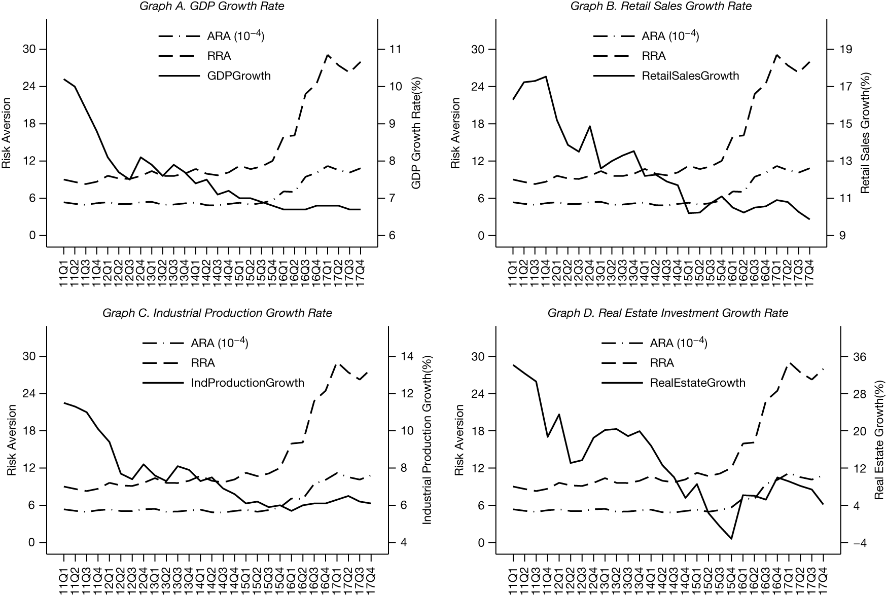
With continuous measures of individuals’ risk aversion, we can first examine whether risk aversion fluctuates over time at the aggregate level.Footnote ⁶ Since our final sample is an approximately representative sample of all the motor vehicle users in China, we measure aggregate risk aversion by averaging the estimated risk aversion measures across all applicants. In Figure 2, we plot the aggregate ARA and RRA together with macroeconomic indicators, including the aggregate GDP growth rate, aggregate retail sales growth rate, aggregate industrial production growth rate, and aggregate real estate investment growth rate. In Graph A, we can see that aggregate ARA was nearly unchanged at around 0.0005 before 2014 but began to increase in late 2015 and doubled to about 0.0010 in 2017. Aggregate RRA slightly fluctuated from 8 to 10 before 2015 but increased rapidly in 2016 and fluctuated between 25 and 30 in 2017. Meanwhile, the aggregate quarterly GDP growth rate of China kept decreasing, although not monotonically, from 2011 to 2017, with a minimum of 6.7% in late 2016 and late 2017. Graph B shows that the quarterly growth rate of aggregate retail sales dropped from around 17% in 2011 to below 11% in 2016 and 2017. In Graph C, we see that the quarterly growth rate of aggregate industrial production also dropped from above 10% in 2011 to around 6% after 2015, with a minimum of 5.7% in the first quarter of 2016, when both aggregate ARA and aggregate RRA began to increase rapidly. Again, as shown in Graph D, aggregate real estate investment increased substantially, with a growth rate higher than 30% in the first half of 2011, and then slowed down. In late 2015, the quarterly growth rate of aggregate real estate investment turned negative and then reversed. Across these graphs, we find that macroeconomic indicators vary earlier and, more importantly, counter to risk aversion. The lagged reaction of risk aversion might be attributable to the general insensitivity of individuals to macroeconomic variations. Figure 2 thus offers preliminary evidence that risk aversion is time-varying and countercyclical, as judged from its countervariation with macroeconomic indicators.

FIGURE 2Average Risk Aversion and Quarterly Macro Indicators

Figure 2 shows the average risk aversion with quarterly macro indicators. The dash-dotted line denotes absolute risk aversion (ARA), and the dashed line denotes relative risk aversion (RRA). The solid line denotes the quarterly growth rate of aggregate GDP in Graph A, the quarterly growth rate of aggregate retail sales in Graph B, the quarterly growth rate of aggregate industrial production in Graph C, and the quarterly growth rate of aggregate real estate investments in Graph D. The absolute risk aversion of each applicant in each quarter is measured using the method of Cohen and Einav (Reference Cohen and Einav2007). Relative risk aversion is the product of absolute risk aversion and the annual per capita consumption of the city in which the applicant lives. We average ARA and RRA across all applicants in each quarter. The sample is from the first quarter of 2011 to the fourth quarter of 2017.

FIGURE 2 Long description

A four-panel line graph set. Each panel shares a common horizontal x-axis representing time from 11 Q 1 to 17 Q 4 and a primary vertical y-axis on the left for Risk Aversion scaled from 0 to 30. A secondary y-axis on the right measures the specific macro indicator growth rate in percentage.

* Graph A. G D P Growth Rate: The solid line for G D P growth starts high at approximately 10 percent and trends downward to 7 percent. The dash-dotted A R A (10 super -4) and dashed R R A lines remain relatively flat until 2016, where they both show a significant upward spike.

* Graph B. Retail Sales Growth Rate: The solid line for retail sales growth fluctuates between 11 and 18 percent, showing a general decline over the period. A R A and R R A follow the same pattern as Graph A, remaining stable before rising sharply in the final two years.

* Graph C. Industrial Production Growth Rate: The solid line for industrial production growth starts near 12 percent, drops to around 6 percent by 2015, and stabilizes. A R A and R R A trends are consistent with previous panels, showing a late-period surge.

* Graph D. Real Estate Investment Growth Rate: The solid line for real estate growth shows the most volatility, starting near 34 percent, dropping sharply to a trough near 0 percent in 2015, and recovering slightly to 8 percent. A R A and R R A lines mirror the other graphs, indicating an inverse relationship with the macro indicator during the 2016 to 2017 period.

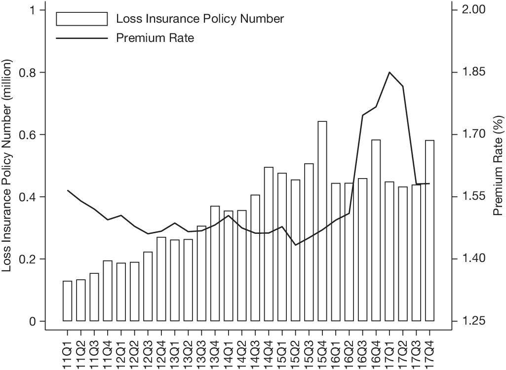
Unlike the cross-sectional variation in risk aversion, the time-varying measure may be influenced by changes in aggregate auto insurance prices over time. For primary auto loss insurance in China, the default deductible rate is 15%. Individuals have the option to choose a policy with a zero-deductible rate and an additional premium, which is 15% of the primary loss insurance premium. Thus, the price of the deductible choice is proportional to the price of the primary loss insurance. To address the concern regarding an aggregate price effect on individuals’ deductible choice and risk aversion measures over time, we plot the number of loss insurance policies and the average premium rate in Figure 3. The figure shows that loss insurance policies increased steadily before 2014 but remained unchanged each year after 2015, although loss insurance sales are higher in the fourth quarter relative to other quarters. Regarding the loss insurance price, the average premium rate fluctuated around 1.5% before the second quarter of 2016 and then increased to about 1.85% in the first quarter of 2017 and decreased afterward. Even though the aggregate loss insurance price changed over time, meaning that the aggregate deductible choice price changed over time, indeed, we do not find a clear comovement between risk aversion measures and the insurance price. In addition, the loss insurance premium is included in the estimation procedure of individuals’ risk aversion parameter. For these reasons, aggregate-level time-varying and countercyclical risk aversion is unlikely to be explained by changes in auto insurance prices.

FIGURE 3Number of Loss Insurance Policies and Average Premium Rate

Figure 3 shows the number of loss insurance policies and the average premium rate in each quarter. The left axis shows the number of loss insurance policies in millions. The right axis shows the average premium rate, which is defined as the loss insurance premium divided by the loss coverage for each policy. The sample is from the first quarter of 2011 to the fourth quarter of 2017.

FIGURE 3 Long description

A combination bar and line graph. The horizontal X axis represents time in quarters from 11 Q 1 to 17 Q 4. The left vertical Y axis measures Loss Insurance Policy Number in millions from 0 to 1. The right vertical Y axis measures Premium Rate as a percentage from 1.25 to 2.00.

* Loss Insurance Policy Number (Bar Chart): Shows a consistent upward trend. Starting at approximately 0.12 million in 11 Q 1, the bars rise steadily to reach a peak of roughly 0.65 million in 15 Q 4, before stabilizing between 0.4 and 0.6 million through 2017.

* Premium Rate (Line Graph): Displays a more volatile trend. It begins at approximately 1.56 percent in 11 Q 1, gradually declining to a low of about 1.43 percent in 15 Q 2. Following this trough, the rate spikes sharply, reaching its highest peak of approximately 1.85 percent in 17 Q 1, before dropping back to around 1.58 percent by 17 Q 4.

A legend at the top left identifies the white bars as Loss Insurance Policy Number and the solid black line as Premium Rate.

B. Individual-Level Regressions

In Section III, we have shown that aggregate risk aversion can fluctuate over time as well as in the opposite direction of economic trends, which are evaluated by macroeconomic indicators. To study the quantitative relationship between individuals’ risk aversion and economic indicators, we further estimate panel regressions with the GDP growth rate and with alternative economic indicators at the individual level.

1. Baseline Findings

The key dependent variable of interest here is RRA. One potential caveat involves the estimation error of RRA because we estimate RRA by the product of ARA and the per capita annual consumption of the city instead of the individual’s annual consumption. Thus, the estimated slope coefficient of GDPGrowth might be biased when the dependent variable is RRA. To address this concern, we additionally use the natural logarithm of RRA as the dependent variable. When the ratio of the individual’s consumption to the per capita consumption of the city is independent and identically distributed (IID) and fixed effects (individual fixed effects, city fixed effects, or time fixed effects) are controlled, the estimated slope coefficient of GDPGrowth is unbiased. See Supplementary Material IA.2 for details.

Table 5 reports the results of both regression models with the dependent variable being the raw estimated risk aversion and the natural logarithm of estimated risk aversion. Unless stated otherwise, all $ t $ -statistics in the panel regressions of the person-quarter panel are adjusted with standard errors clustered by both province and year $ \times $ quarter and account for correlations across individuals, autocorrelations, and other correlations within the province. In Panel A, we control for the individual’s person fixed effects. Similar to Pástor, Stambaugh, and Taylor (Reference Pástor, Stambaugh and Taylor2017), the ordinary least squares estimator controlling for person fixed effects is a weighted average across individuals of the slope coefficients from person-to-person time-series regressions and thus reflects only the time-series variation in risk aversion and the GDP growth rate. It also absorbs the potential effect of time-invariant personal characteristics, such as demographics and wealth endowment, on risk aversion. In column 1, the regression coefficient of GDPGrowth is −86.739, statistically significant with a $ t $ -statistic of −3.74, meaning that the individual’s ARA is negatively correlated with the GDP growth rate. When we use the natural logarithm of ARA as the dependent variable in column 2, the estimated coefficient is −13.602 with a $ t $ -statistic of −3.08. This means that a 1-standard-deviation decline in the quarterly GDP growth rate is associated with a 24.5% increase in the individual’s ARA. For the individual’s RRA, column 4 shows it to be negatively correlated with the GDP growth rate, with an estimated coefficient of −20.340 and statistically significant at the 1% level. The magnitude of the coefficient means that a 1-standard-deviation decline in the quarterly GDP growth rate is associated with a 36.6% increase in RRA. The level regression in column 3 is consistent: the estimated coefficient is −293.244, statistically significant at the 1% level, corresponding to an increase of 5.3 in RRA, though this level estimate is subject to the consumption-proxy bias. The results show that the time-series negative correlation between an individual’s risk aversion and the GDP growth rate is both statistically and economically significant.

TABLE 5Regressions of Risk Aversion on GDP Growth Rate

TABLE 5 Long description

The table consists of four columns of data labeled 1 through 4. The column headers are A R A, L n open parenthesis A R A close parenthesis, R R A, and L n open parenthesis R R A close parenthesis.

Panel A. Person Fixed Effect

G D P Growth coefficients are negative and statistically significant at the 1 percent level across all columns: -86.739 for A R A, -13.602 for L n A R A, -293.244 for R R A, and -20.340 for L n R R A. T-statistics range from -3.08 to -3.93. Number of observations is 10,229,255 for A R A and 8,997,276 for R R A. Within R-squared values range from 0.011 to 0.068.

Panel B. Province Fixed Effect

G D P Growth coefficients remain negative and significant at the 1 percent level: -68.413 for A R A, -15.210 for L n A R A, -242.217 for R R A, and -21.839 for L n R R A. T-statistics range from -3.79 to -4.76. Observation counts are identical to Panel A. Within R-squared values range from 0.010 to 0.026.

Panel C. Person and Year times Quarter Fixed Effects

G D P Growth coefficients are no longer statistically significant. Values are -15.154 for A R A, 0.876 for L n A R A, -25.950 for R R A, and 1.507 for L n R R A. T-statistics range from -1.48 to 0.38. Within R-squared values are near zero (0.001 or 0.000).

Panel B reports the results of panel regressions controlling for the province fixed effects. The regression coefficient essentially captures the average covariation in risk aversion and the GDP growth rate within the province. However, there is no cross-sectional variation in the GDP growth rate within the province, meaning that the regression coefficient captures the average time-series correlation between risk aversion and the GDP growth rate within the province. Therefore, controlling for province fixed effects could help verify the estimated time-series correlation of risk aversion and the GDP growth rate in Panel A. Columns 1 and 2 show that, consistent with the previous findings, the time-series correlation between the individual’s ARA and the GDP growth rate within the province is significantly negative. The estimated coefficients of GDPGrowth are −68.413 and −15.210, which are statistically significant. When we use the raw RRA as the dependent variable in column 3, the estimated coefficient is −242.217 with a $ t $ -statistic of −4.10. In column 4, the estimated coefficient of GDPGrowth on the natural logarithm of RRA is −21.839 and statistically significant ( $ t $ -stat = −4.76). Considering the economic significance, columns 2 and 4 show that, within the province, a 1-standard-deviation decline in the quarterly GDP growth rate is associated with a 27.4% increase in the individual’s ARA and a 39.3% increase in RRA. In sum, the time-series negative correlation between the individual’s risk aversion and the GDP growth rate within the province remains significant and is larger in economic magnitude.

The aforementioned results show a quantitatively negative relation between risk aversion and the GDP growth rate in the time series, providing direct support for time-varying and countercyclical risk aversion, which is the main empirical result of the article. To further investigate the extent to which risk aversion varies inversely with economic trends, we estimate panel regressions controlling for both person and quarter fixed effects in Panel C. Compared with the panel regression controlling for the person fixed effects, the addition of time fixed effects would additionally control for the aggregate variation in variables over time but not the variation across individuals. Intuitively, the slope coefficient reflects the time-series relation of risk aversion and the GDP growth rate after deducting the aggregate economic trends effect. In Panel C, the estimated coefficients of GDPGrowth contract drastically in magnitude and are statistically indistinguishable from 0 for both absolute and RRA. This means that the time-series negative correlation between the individual’s risk aversion and the GDP growth rate is almost entirely explained by changes in aggregate economic trends.

2. Evidence Against Mechanical Explanations

As discussed in Section II, the risk aversion formula in equation (5) maps each individual’s deductible choice into an ARA estimate through the expected-loss moments $ E(L) $ and $ E\left({L}^2\right) $ and the premium rate $ {p}_i^0 $ (the price of the zero-deductible add-on, equal to 15% of the primary premium divided by coverage). This mapping raises the concern that the countercyclical pattern could be mechanically induced rather than reflecting genuine preference variation. First, if $ E(L) $ or $ E\left({L}^2\right) $ varies cyclically (e.g., with road conditions or repair cost inflation) or geographically, the estimated risk aversion could inherit that variation. Second, because the add-on price is a fixed proportion of the base premium, any cyclical movement in premiums passes into $ {p}_i^0 $ , and a higher $ {p}_i^0 $ mechanically implies a higher inferred $ r $ , so cyclical pricing could masquerade as countercyclical risk aversion. Third, the changing composition of insured vehicles over time could confound the relationship if vehicle age correlates with both pricing and the business cycle. We subsequently address all three concerns: the first two by reestimating individual risk aversion via the Gibbs sampler under alternative inputs (Table 6) and the third by restricting the sample to narrow vehicle age bands (Table 7).

TABLE 6Risk Aversion on GDP Growth Rate: Evidence Against Mechanical Explanations

TABLE 6 Long description

The table consists of four panels (A, B, C, and D) with four columns each. The columns are labeled 1: A R A, 2: Ln(A R A), 3: R R A, and 4: Ln(R R A). All panels use G D P Growth as the independent variable and include Person fixed effects.

Panel A (Year-Specific): G D P Growth coefficients are -223.047 (t-stat -4.53) for A R A, -22.393 (t-stat -2.78) for Ln(A R A), -661.841 (t-stat -4.07) for R R A, and -28.557 (t-stat -3.44) for Ln(R R A).

Panel B (Year-Quarter-Specific): G D P Growth coefficients are -298.789 (t-stat -3.61) for A R A, -29.957 (t-stat -3.16) for Ln(A R A), -877.869 (t-stat -3.36) for R R A, and -36.848 (t-stat -3.71) for Ln(R R A).

Panel C (Province-Specific): G D P Growth coefficients are -449.655 (t-stat -3.88) for A R A, -65.928 (t-stat -6.03) for Ln(A R A), -1,317.626 (t-stat -3.45) for R R A, and -72.770 (t-stat -5.81) for Ln(R R A).

Panel D (First-Policy Premium Rate): G D P Growth coefficients are -124.527 (t-stat -7.65) for A R A, -33.301 (t-stat -7.00) for Ln(A R A), -383.223 (t-stat -5.93) for R R A, and -39.769 (t-stat -7.82) for Ln(R R A).

All G D P Growth coefficients across all panels are statistically significant at the 1 percent level, indicated by three asterisks. The number of observations is 10,229,255 for A R A columns and 8,997,276 for R R A columns.

TABLE 7Countercyclical Risk Aversion across Narrow Car-Age Bands

TABLE 7 Long description

The table consists of four columns of dependent variables: 1 A R A, 2 Ln A R A, 3 R R A, and 4 Ln R R A. All panels use Person fixed effects.

Panel A. Car Aged 1 to 3 Years:

* G D P Growth coefficients: -5.431, -3.556, -66.281 (significant at 1 percent), and -8.456 (significant at 1 percent).

* Number of Observations: 3,015,747 for A R A and 2,546,646 for R R A.

* Within R-squared: 0.000 to 0.011.

Panel B. Car Aged 4 to 6 Years:

* G D P Growth coefficients: -51.636 (significant at 10 percent), -14.430 (significant at 5 percent), -211.553 (significant at 5 percent), and -21.365 (significant at 1 percent).

* Number of Observations: 1,180,650 for A R A and 1,036,650 for R R A.

* Within R-squared: 0.006 to 0.024.

Panel C. Car Aged 7 to 9 Years:

* G D P Growth coefficients: -186.427 (significant at 10 percent), -30.955 (significant at 5 percent), -681.361 (significant at 5 percent), and -42.628 (significant at 1 percent).

* Number of Observations: 283,455 for A R A and 256,914 for R R A.

* Within R-squared: 0.018 to 0.044.

Across all panels, the magnitude of the negative coefficients for G D P Growth increases as the car age increases.

We first address the expected-loss concern. We replace the full-sample $ E(L) $ and $ E\left({L}^2\right) $ with time- or geography-adjusted values and rerun the entire Gibbs sampling procedure from scratch. Specifically, we consider three specifications: i) year-specific $ {E}_t(L) $ and $ {E}_t\left({L}^2\right) $ computed from claims in each calendar year, ii) year-quarter-specific $ {E}_t(L) $ and $ {E}_t\left({L}^2\right) $ computed from claims in each quarter, and iii) province-specific $ {E}_p(L) $ and $ {E}_p\left({L}^2\right) $ computed from claims in each province. We then rerun the main GDP growth regressions from Table 5 using each set of reestimated measures. Panels A–C of Table 6 report the GDP growth coefficients, all controlling for person fixed effects. In Panel A (year-specific $ {E}_t(L) $ ), Panel B (year-quarter-specific $ {E}_t(L) $ ), and Panel C (province-specific $ {E}_p(L) $ ), the coefficient on GDP growth is negative and statistically significant across all dependent variables.Footnote ⁷ Replacing the full-sample expected-loss moments with time- or geography-adjusted values therefore does not change the countercyclical pattern.

We next address the premium-rate concern with an experiment that removes any within-person time variation in the premium rate. We reestimate risk aversion via the full Gibbs sampler with each individual’s premium rate $ {p}_i^0 $ held fixed at its first-policy value across all of the individual’s policies. Panel D of Table 6 reports the results. The coefficient on GDP growth remains negative and statistically significant across all four risk aversion measures, indicating that the countercyclical pattern is unlikely to be mechanically driven by cyclical movements in the premium rate.Footnote ⁸ We caution that this is an illustrative experiment rather than a counterfactual reestimation: holding $ {p}_i^0 $ at a counterfactual value changes the price the individual faces, at which the optimal deductible choice could itself differ, yet we continue to treat the observed deductible choice as data.Footnote ⁹ This inconsistency biases the level of the reestimated risk aversion, so the exercise is best interpreted as a diagnostic of whether the countercyclical pattern survives when the premium rate is held fixed, not as a structurally interpretable estimate of its magnitude.

We finally consider the concern that vehicle composition changes over time: if newer vehicles carry systematically different pricing or deductible choices, shifts in the vehicle age distribution could confound the relationship between risk aversion and macroeconomic conditions. We therefore restrict the sample to narrow car-age bands—vehicles aged 1–3, 4–6, and 7–9 years—and reestimate the main specification within each band, holding vehicle age approximately constant. Table 7 reports the results. The countercyclical pattern persists across all three bands and strengthens for older vehicles: the coefficient on Ln(RRA) rises in magnitude to $ -42.628 $ ( $ t=-2.60 $ ) in the 7–9-year band. If the pattern were driven by mechanical coverage dynamics, the effect should be weaker for older cars, which have lower replacement values; the opposite gradient is more consistent with genuine preference variation.

Taken together, these analyses provide evidence against the most plausible mechanical explanations for the countercyclical pattern—cyclical loss moments, premium-rate movements, and vehicle composition. We nonetheless emphasize a limitation of our design. As Panel C of Table 5 shows, the GDPGrowth coefficient becomes statistically indistinguishable from 0 once common year $ \times $ quarter fixed effects are included, so identification ultimately rests on aggregate time-series variation. As a result, we cannot fully rule out other market-wide changes, such as underwriting, contract menus, or sales practices, that coincide with the business cycle and could affect the insurance-implied risk aversion measure. We view such confounds as unlikely to reproduce the breadth of patterns we document, but the present design cannot eliminate them entirely.

A. Seasonality in Risk Aversion

The link between seasons and risk aversion is based on the view that a seasonal reduction in daylight hours can lead to a marked deterioration in people’s moods and is also based on clinical evidence that a dampened mood can have a negative influence on risk-taking behavior (Kamstra et al. (Reference Kamstra, Kramer, Levi and Wermers2017)). The incidence of depression is linked with SAD because of the seasonal reduction in daylight hours. In addition, healthy people could also suffer a milder but still problematic disorder, commonly called “winter blues” (Kamstra et al. (Reference Kamstra, Kramer and Levi2003), Kramer and Weber (Reference Kramer and Weber2012)). Existing studies have documented seasonal patterns in the returns of stocks and bonds, the movement of money between mutual fund categories, both consistent with seasonally varying risk preferences (Kamstra et al. (Reference Kamstra, Kramer and Levi2003), (Reference Kamstra, Kramer and Levi2015), (Reference Kamstra, Kramer, Levi and Wermers2017), Garrett et al. (Reference Garrett, Kamstra and Kramer2005)). Kamstra, Kramer, Levi, and Wang (Reference Kamstra, Kramer, Levi and Wang2014) also developed an asset pricing model with a representative agent experiencing seasonally varying risk preferences and generated the empirically observed seasonal patterns in equity and Treasury returns.

In this section, we examine seasonality in risk aversion with our measures. We follow Kamstra et al. (Reference Kamstra, Kramer and Levi2003) to measure the effect of SAD by the number of nighttime hours from sunset to sunrise during the fall and winter. We first calculate the sun’s declination angle at day $ t $ as $ {\lambda}_t=0.4102\times \mathit{\sin}\left(\frac{2\pi }{365}\times \left({Julian}_t-80.25\right)\right) $ , where $ {Julian}_t $ is the number of the day in the year, which ranges from 1 to 365 (366 in a leap year). Since all cities in our sample are in the Northern Hemisphere, we then calculate the number of nighttime hours as $ {SAD}_t=12-7.72\times \mathit{\operatorname{arccos}}\left(-\mathit{\tan}\left(\frac{2\pi \delta}{360}\right)\mathit{\tan}\left({\lambda}_t\right)\right) $ , where $ \delta $ is the latitude of the city in which the applicant lives. The $ {SAD}_t $ measure is set to be 0 in the spring and summer. We also include a dummy variable for the fall and winter. The results are reported in Table 8. City and year fixed effects are included in all specifications to control for the variations in risk aversion across cities and years.

TABLE 8Seasonally Varying Risk Aversion

TABLE 8 Long description

Panel A. Absolute Risk Aversion (A R A).

This panel presents six regression models. Models 1 to 3 use A R A as the dependent variable, and models 4 to 6 use Natural Logarithm of A R A.

* S A D: Coefficients are 0.336 (t-stat 3.59) in model 1, 0.271 (t-stat 2.47) in model 3, 0.061 (t-stat 3.25) in model 4, and 0.052 (t-stat 2.56) in model 6.

* Fall forward slash Winter: Coefficients are 0.474 (t-stat 4.53) in model 2, 0.132 (t-stat 3.42) in model 3, 0.085 (t-stat 3.71) in model 5, and 0.020 (t-stat 3.04) in model 6.

* Fixed effects: City and year for all models.

* Number of Observations: 10,166,390.

* Within R-squared: Ranges from 0.048 to 0.062.

Panel B. Relative Risk Aversion (R R A).

This panel presents six regression models. Models 1 to 3 use R R A as the dependent variable, and models 4 to 6 use Natural Logarithm of R R A.

* S A D: Coefficients are 0.769 (t-stat 2.89) in model 1, 0.643 (t-stat 2.11) in model 3, 0.062 (t-stat 3.07) in model 4, and 0.053 (t-stat 2.40) in model 6.

* Fall forward slash Winter: Coefficients are 1.072 (t-stat 3.53) in model 2, 0.259 (t-stat 2.79) in model 3, 0.086 (t-stat 3.53) in model 5, and 0.018 (t-stat 2.42) in model 6.

* Fixed effects: City and year for all models.

* Number of Observations: 8,997,276.

* Within R-squared: Ranges from 0.067 to 0.100.

In Panel A, column 1 shows that ARA appears to be positively correlated with the SAD measure with a coefficient of 0.336, which is statistically significant with a $ t $ -statistic of 3.59. In column 2, the indicator variable for fall and winter is statistically significant with a coefficient of 0.474 and a $ t $ -statistic of 4.53. We jointly estimate a regression of ARA on the SAD measure and the indicator variable for fall and winter in column 3; both coefficients decrease in magnitude but remain statistically significant. When we use the natural logarithm of ARA as the dependent variable in columns 4–6, the results also show a positive correlation between ARA and the SAD measure and indicate that individuals’ ARA is statistically higher in the fall and winter. We then reestimate the regression of RRA in Panel B. In columns 1 and 2, the coefficient of SAD is 0.769, and the coefficient of the indicator variable for fall and winter is 1.072 in the univariate regression, and both are statistically significant. We interpret the economic magnitudes in the multivariate regression in column 3 as follows: First, the SAD measure is significant with a coefficient of 0.643 and a $ t $ -statistic of 2.11, meaning that a 1-hour increase in nighttime hours in the fall and winter is associated with an increase in the RRA coefficient of 0.643. Second, the coefficient of the indicator variable for fall and winter is 0.259, remaining significant. Since the mean of the SAD measure in the fall and winter is 1.264, an average individual’s RRA is 1.072 ( $ 0.259+1.264\times 0.643 $ ) higher in the fall and winter than in the spring and summer. This magnitude is the same as the coefficient in the univariate regression in column 2. In columns 4–6, the correlations of both the SAD measure and the indicator variable for fall and winter with individuals’ RRA are also positive and statistically significant, consistent with the results of level regressions. Overall, the results are consistent with individuals’ risk aversion increasing with the length of the night and being higher in the fall and winter.

B. Zodiac Years

We follow Fisman et al. (Reference Fisman, Huang, Ning, Pan, Qiu and Wang2023) to investigate the role of superstition, specifically the “zodiac year effect,” in the variation in risk aversion. In China, the zodiac year is the year when each person’s age is a multiple of 12. The zodiac year effect refers to the superstitious belief that people are at risk of encountering misfortunes in the zodiac year and therefore are more cautious when making decisions under uncertainty. To gain some insight into the plausibility of individuals’ superstition affecting their level of risk aversion, we test risk aversion fluctuations around the zodiac year.

In Table 9, we estimate panel regressions of risk aversion measures on the zodiac year indicator, controlling for demographic variables and car attributes. Odd-numbered columns include year fixed effects, and even-numbered columns add person fixed effects to exploit within-individual variation in zodiac year status. In the year fixed effects regressions, we find that individuals who are in their zodiac year have a 1.5% higher level of ARA and a 1.6% higher level of RRA than others, and both coefficients are statistically significant after controlling for demographic variables and car attributes. With person and year fixed effects, the zodiac year effect remains positive and statistically significant for logarithm risk aversion measures. The zodiac year is associated with a 0.5% higher Ln(ARA) ( $ t $ -stat = 4.58) and a 0.4% higher Ln(RRA) ( $ t $ -stat = 4.61), consistent with the zodiac year effect reflecting within-individual variation rather than cross-sectional composition effects. These results support the hypothesis that psychological forces could lead to time-varying risk aversion; in this case, an individual’s level of risk aversion is higher in the zodiac year every 12 years, consistent with superstitious beliefs.

TABLE 9Risk Aversion in Zodiac Years

TABLE 9 Long description

A regression table with 8 columns. The top header row lists four dependent variables, each covering two columns: A R A (columns 1 and 2), Ln(A R A) (columns 3 and 4), R R A (columns 5 and 6), and Ln(R R A) (columns 7 and 8).

Key independent variables and their coefficients (t-statistics in parentheses):

* Zodiac: Shows positive coefficients across all models, ranging from 0.004 to 0.318, all statistically significant at the 1% or 5% level.

* Male: Positive coefficients in odd-numbered columns (0.399 for A R A and 0.795 for R R A); omitted in even-numbered columns.

* Age: Generally positive and significant coefficients, except in column 8.

* LnExpense: Positive and highly significant coefficients across all models.

* LnCoverage: Negative and highly significant coefficients across all models.

* CarAge: Generally negative and significant coefficients.

Bottom rows specify model details:

* Fixed effect: Odd columns use Year; even columns use Person and Year.

* No. of Obs.: Ranges from approximately 8.16 million to 9.80 million.

* Within R-squared: Ranges from 0.074 to 0.613.

C. Risk Aversion Around Calendar Events

Stock returns on trading days before holidays are abnormally high: 9–14 times higher than ordinary-day returns across U.S. exchanges and international markets (Ariel (Reference Ariel1990), Kim and Park (Reference Kim and Park1994)), and the pattern persists over 90 years of data (Lakonishok and Smidt (Reference Lakonishok and Smidt1988)). The leading explanation is that the anticipation of leisure and festivity elevates mood, which in turn shifts risk attitudes (Meier (Reference Meier2022)). Our individual-level risk aversion measures allow us to examine this channel by tracing how risk preferences vary around calendar events.

We conduct event studies around China’s major national holidays: National Day (October 1–7, a week-long “Golden Week” of collective celebration and mass travel), Workers’ Day (May 1, leisure and public festivities), Spring Festival (Chinese New Year, a 7-day holiday that coincides with the bonus season), and New Year’s Day (January 1, coinciding with the fiscal year-end). We restrict the sample to policies issued within 1 week before each event, during the event, and 1 week after, and estimate panel regressions of risk aversion on indicators for the event period (Event) and the post-event week (Post1w), with the pre-event week as the benchmark. All regressions include person and year fixed effects.

Table 10 reports the results. When we pool four holidays (columns 1–4), the logarithm risk aversion measures are significantly higher during the holiday period: Ln(ARA) increases by 0.066 ( $ t=3.06 $ ) and Ln(RRA) by 0.060 ( $ t=2.80 $ ) relative to the pre-holiday week. The effect persists into the post-holiday week, with coefficients of 0.034 ( $ t=2.55 $ ) for Ln(ARA) and 0.035 ( $ t=2.70 $ ) for Ln(RRA), suggesting that the holiday effect does not disappear immediately.Footnote ¹² When we examine two holidays that coincide with fiscal year-ends and bonus seasons, New Year’s Day (columns 5–8) shows no significant effect on any measure of risk aversion, and Spring Festival (columns 9–12) is similarly not statistically significant.Footnote ¹³

TABLE 10Risk Aversion Around Calendar Events

TABLE 10 Long description

The table is organized into three main header groups: Four Holidays (Columns 1 to 4), Fiscal Year-End: New Year (Columns 5 to 8), and Bonus Season: Spring Festival (Columns 9 to 12). Each group contains four dependent variables: A R A, Ln(A R A), R R A, and Ln(R R A).

Key row variables include:

* Event: Shows a significant positive coefficient for Ln(A R A) at 0.066 and Ln(R R A) at 0.060 in the pooled Four Holidays group.

* Post 1 w: Shows significant positive coefficients for Ln(A R A) at 0.034 and Ln(R R A) at 0.035 in the pooled group.

* Age: Shows a highly significant positive coefficient for A R A at 3.774 and R R A at 12.751 specifically during the Bonus Season.

* LnExpense: Shows consistently positive and highly significant coefficients across all twelve columns, ranging from 4.941 to 15.920.

* LnCoverage: Shows consistently negative and highly significant coefficients across all columns, ranging from minus 29.182 to minus 87.199.

* CarAge: Shows generally negative coefficients, significant in the pooled and bonus season columns.

Bottom rows indicate that all specifications include Person F E and Year F E. The number of observations ranges from 97,843 to 890,167. Within R-squared values range from 0.071 to 0.356. T-statistics are provided in parentheses below coefficients.

These associations are consistent with a mood and affect channel: National Day and Workers’ Day—holidays centered on collective celebration and routine disruption—are associated with elevated risk aversion, much as seasonal darkness is associated with mood and risk preferences in the SAD analysis of Section V.A.

Together with the zodiac year finding in Section V.B, these analyses are consistent with psychological forces—seasonal mood, culturally embedded beliefs, and holiday-related emotional states—correlating with individual risk aversion over time.