1. Introduction
Over the past few decades, inflation has remained low and relatively stable in most advanced economies and a growing number of emerging economies. This development is often associated with the widespread adoption of inflation-targeting (IT) regimes, which the empirical literature typically characterizes as following a Taylor rule (see, e.g., Taylor and Davradakis, Reference Taylor and Davradakis2006; Çağlayan and Astar, Reference Çağlayan and Astar2010; Neuenkirch and Tillmann, Reference Neuenkirch and Tillmann2014).Footnote 1 By committing to an explicit inflation target and typically granting the central bank sufficient independence to pursue this objective, many countries were able to mitigate the time-inconsistency problem in monetary policy. In the absence of credible rules, policymakers often succumb to the temptation of expansionary monetary policies for short-term gains—such as monetizing fiscal deficits, exploiting short-run Phillips-curve trade-offs, or stimulating investment through lower interest rates. These policies typically lead to rising inflation, which in turn undermines growth, as illustrated most clearly by the stagflation experienced across many advanced economies in the 1970s. Yet, the empirical evidence on the growth effects of IT remains inconclusive. One reason may be that not all IT regimes are created equal. For example, El-Shagi and Ma (Reference El-Shagi and Ma2023) document that most IT countries do not satisfy the Taylor principle: policy rates do not increase more than proportionally with inflation expectations, so real interest rates fail to rise, thereby preventing monetary policy from becoming genuinely contractionary. In this paper, we contribute to this literature by examining how the central bank’s commitment to price stability—proxied by the long-run inflation coefficient in an estimated Taylor rule—affects economic growth. Since country fixed effects are a key component of a well-specified empirical growth model, we cannot exploit cross-country variation in the Taylor rule. Instead, we exploit the time variation in monetary policy rules documented in recent work.
We thus contribute to two strands of the literature. First, we add to the empirical literature on the growth effects of monetary policy. While there is a large body of work on how monetary policy regimes—including inflation targeting—shape growth, to the best of our knowledge ours is the first paper to examine how the implementation of a common policy rule in practice affects growth. Second, we extend the literature on time-varying estimates of monetary policy reaction functions (MPRF). A considerable empirical literature has explored time-varying monetary policy reaction functions—typically Taylor rules—for the Federal Reserve, the ECB, and a range of smaller economies. Yet relatively few studies analyze a broad cross-section of countries using a consistent and comparable empirical framework. A notable exception is the study by Anderl and Caporale (Reference Anderl and Caporale2024), who employ a time-varying GMM approach to estimate forward-looking Taylor rules for ten developed economies, using the estimation strategy introduced by Partouche (Reference Partouche2007). Although our ultimate goal is to assess growth effects rather than to analyze time variation in policy rules per se, our sample of 37 IT countries makes this the most comprehensive study to date in this line of empirical research.
Our findings indicate sizable and statistically robust effects of a more hawkish policy stance on economic growth, with annual impacts ranging from 0.8% to 1.7% across specifications. The growth benefits typically associated with inflation targeting are largely confined to countries that react more forcefully to inflation, implying that adopting an inflation-targeting label alone is insufficient. This underscores the importance of the intensity of policy reactions and suggests that even widely regarded “best-practice” monetary frameworks remain vulnerable to time-inconsistency problems that can undermine growth outcomes.
The remainder of this paper is structured as follows. The next section summarizes the literature. Section 3 introduces our research methodology, and Section 4 discusses the results. Finally, Section 5 concludes.
2. Literature review
2.1 Monetary policy and growth
The previous literature approaches the impact of monetary policy on growth from two fundamentally distinct perspectives. One strand, the literature on monetary neutrality, examines whether expansionary and contractionary monetary policy have persistent effects on output. The other strand focuses on institutional determinants of growth, analyzing how central bank features such as inflation targeting, central bank independence, and related governance arrangements shape economic performance. Both strands report mixed empirical findings.
Both King and Watson (Reference King and Watson1997) and Bernanke and Mihov (Reference Bernanke and Mihov1998) find that US postwar data is consistent with the neutrality – but not the superneutrality—of money. Yet Mankiw (Reference Mankiw2001) interprets the very findings of Bernanke and Mihov (Reference Bernanke and Mihov1998) as evidence of non-neutrality. More recently, Jordà et al. (Reference Jordà, Singh and Taylor2024) find that expansionary policy is neutral, whereas contractions leave permanent scars that reduce output. Serletis and Xu (Reference Serletis and Xu2024) emphasize that, for most countries, the data does not even permit meaningful tests of neutrality, but they confirm neutrality where such tests are feasible. Serletis and Koustas (Reference Serletis and Koustas1998) test the neutrality and superneutrality of money for ten developed countries and find neutrality in all cases and superneutrality in all but Italy. Italy stands out as the only country in their sample experiencing a persistent shock to money growth. This link between persistent money-growth shocks (and thus persistent changes to inflation) and the failure of superneutrality connects their findings to the broader literature on the growth effects of inflation (Bick, Reference Bick2010; López-Villavicencio and Mignon, Reference López-Villavicencio and Mignon2011), and, by extension, to the literature on how central bank institutions influence growth through their role in maintaining price stability.
Much of this work focuses on inflation targeting and central bank independence. For inflation targeting, some studies find that it can support long-run growth by anchoring expectations and reducing macroeconomic volatility (Mishkin, Reference Mishkin2007; Svensson, Reference Svensson2010), whereas others report little or no effect (Ball and Sheridan, Reference Ball and Sheridan2004; Brito and Bystedt, Reference Brito and Bystedt2010; Junankar and Wong, Reference Junankar and Wong2020). The evidence on central bank independence is similarly mixed. While some research argues that greater independence strengthens credibility and fosters growth (Akinci et al. Reference Akinci, Akinci and Yilmaz2015; Garriga, Reference Garriga2016), other studies find no systematic growth benefits (Neyapti, Reference Neyapti2001; de Mendonça, Reference de Mendonça2006; Anastasiou, Reference Anastasiou2009). A related, largely theoretical literature addresses the more fundamental question of which monetary policy framework—understood broadly as the rule or target variable guiding the conduct of policy—delivers the highest economic growth (see, e.g., Lai and Chin, Reference Lai and Chin2013; Chu and Ji, Reference Chu and Ji2016; Huang et al. Reference Huang, Yang and Cheng2017; Chu et al. Reference Chu, Ning and Zhu2019; Gil and Iglésias, Reference Gil and Iglésias2020).
By examining how the operational features of an IT framework shape growth, our paper bridges the two strands of literature on policy actions and institutional or rule-based frameworks. Concretely, we ask how a hawkish versus a dovish stance of the central bank within an IT framework affects growth. Empirical work on this aspect is still scarce. The paper closest to our question is Gil et al. (Reference Gil, Iglésias and Guimaraes2023), who provide theoretical support for the idea that strong policy responses to inflation—which are consistent with the Taylor principle—anchor expectations and create conditions that contribute to growth.
2.2 Time-varying monetary policy reaction functions
Our identification strategy exploits time variation in the Taylor rule. This allows us to estimate the effect of changes in Taylor-rule parameter—particularly the long-run inflation coefficient—on growth, while accounting for time-invariant country heterogeneity through fixed effects. Introducing time variation into estimated versions of the original backward-looking Taylor (Reference Taylor1993) specification is conceptually straightforward (see, e.g., Judd et al. Reference Judd and Rudebusch1998; Assenmacher-Wesche, Reference Assenmacher-Wesche2006; Kuzin, Reference Kuzin2006). However, since the seminal work of Clarida et al. (Reference Clarida, Galí and Gertler1998), it has become widely accepted that central banks typically respond to expected inflation and output rather than to current conditions. Future realizations—often used as proxies for expectations under the rational-expectations assumption—are endogenous to monetary policy by construction, since policy is explicitly designed to influence those future outcomes. Orphanides (Reference Orphanides2001) proposes using real-time forecasts, such as Greenbook or SPF projections, to address this endogeneity concern, since these forecasts are conditioned only on information available at the time and are therefore exogenous to contemporaneous policy shocks. Yet such forecasts are often unavailable, meaning that estimating a forward-looking policy rule requires an instrumental-variables approach that complicates time-varying-parameter estimation. Wesche (Reference Wesche2003) proxies inflation expectations using a VAR-based forecast in her Markov-switching framework, and, in a similar spirit, Trecroci and Vassalli (Reference Trecroci and Vassalli2010) use trend inflation—derived from a simple filtering procedure—as a measure of long-run expectations in his time-varying-parameter model. Both approaches amount to ad hoc modifications of a standard two-stage IV procedure to accommodate evolving monetary-policy parameters. A two-step procedure for estimating bias-corrected, forward-looking, time-varying Taylor rules was introduced by Kim and Nelson (Reference Kim and Nelson2006) and has been applied in various empirical settings, including the Brazilian case examined by Carvalho and Muinhos (Reference Carvalho and Muinhos2023). An alternative approach is the GMM framework proposed by Partouche (Reference Partouche2007), which Anderl and Caporale (Reference Anderl and Caporale2024) apply in their ten-country study. A much larger literature examines time variation in monetary policy using VAR-based approaches (see, e.g., Boivin and Giannoni, Reference Boivin and Giannoni2006; Cogley and Sargent, Reference Cogley and Sargent2005; Primiceri, Reference Primiceri2005; Sims and Zha, Reference Sims and Zha2006). However, these approaches do not permit identification of the policy parameters, rendering them unsuitable for addressing our research question.
In this paper, we employ the framework of Kim and Nelson (Reference Kim and Nelson2006) to model gradual shifts in the reaction function of 37 inflation-targeting countries.
3. Model and estimation strategy
3.1 Panel growth regression model
The model. We augment a standard panel growth regression by including a time-varying measure of policy hawkishness as our main explanatory variable.
Following the usual convention in the growth literature, we construct non-overlapping five-year periods and estimate our model on this quinquennial panel (see, e.g., Barro et al. Reference Barro2003; Bruns and Ioannidis, Reference Bruns and Ioannidis2020):
 \begin{equation} \Delta y_{i,t}= \delta _0 + \delta _1 y_{i,t - 1} + \delta _2 \text{Hawk}_{i,t-1} + \phi X_{i,t} + u_i + v_{t} + \varepsilon _{i,t}, \end{equation}
Here,
 $y_{i,t-1}$
is the log of real GDP per capita at the onset of the period, and
 $\text{Hawk}_{i,t-1}$
is an indicator for whether country
 $i$
exhibited a hawkish policy stance at that time. The vector
 $X_{i,t}$
contains standard growth determinants, including population growth, investment, government consumption (as a share of GDP), education, and trade openness, all measured at the end of period
 $t-1$
, corresponding to the beginning of the period
 $t$
. Country and time fixed effects are captured by
 $u_i$
and
 $v_t$
, and
 $\varepsilon _{i,t}$
is the idiosyncratic error term.
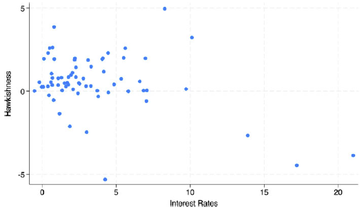
We define hawkishness as a strong response to inflation. In the public debate, this is often reduced to a preference for higher interest rates. This association arises because hawkishness attracts most attention when the trade-off between price stability and growth is most acute—that is, when combating inflation risks undermining economic expansion. However, hawkishness—in the sense of fighting inflation aggressively—is not necessarily associated with higher interest rates. If anything, low equilibrium inflation implies a low equilibrium nominal interest rate, and price stability may further reduce the real interest rate by compressing the average risk premium. Indeed, Figure A.1 shows no discernible correlation between real interest rates and hawkishness at moderate levels—if anything, it is extreme dovishness that tends to coincide with elevated rates. At the same time, expansionary policy offers only transitory support through the Phillips curve—once expectations adjust, the effect dissipates. Adherence to the Taylor principle, by contrast, may deliver permanent price stability. Since high and, more importantly, volatile inflation reduces allocative efficiency, hawkishness in our sense may well be beneficial for long-run growth.
Estimation. The specification in Equation (1) corresponds to an autoregressive process in the log level of GDP and can be rewritten equivalently as:
 \begin{equation} y_{i,t}= \delta _0 + (\delta _1+1) y_{i,t - 1} + \delta _2 \text{Hawk}_{i,t-1} + \phi X_{i,t} + u_i + v_{t} + \varepsilon _{i,t}, \end{equation}
Dynamic panel models such as Equation (2) require estimators that address the endogeneity introduced by the inclusion of the lagged dependent variable. A widely used approach in the growth literature is the system-GMM estimator of Arellano and Bover (Reference Arellano and Bover1995) and Blundell and Bond (Reference Blundell and Bond1998), which leverages additional moment conditions to enhance efficiency, especially when the variable of interest exhibits high persistence.
However, the validity of the assumptions required for system GMM when applied to growth regressions has been questioned, particularly the stationarity requirement for the level equation (Moral-Benito, Reference Moral-Benito2013, Reference Moral-Benito2016). Including country and time fixed effects can absorb much of the non-stationarity, as the stochastic trend in output is largely driven by global shocks to total factor productivity. Indeed, the autoregressive coefficient in Equation (2) is well below unity for almost all estimators we consider, indicating that stationarity is not a major concern. Yet to ensure robustness to the Moral-Benito critique, we rely on several estimation strategies rather than a single method.
First, we consider a standard fixed-effects estimator, which merely captures unobserved heterogeneity through fixed effects and leaves other identification issues unaddressed. Second, we use system-GMM to address potential endogeneity. Third, we employ the difference-GMM estimator of Arellano and Bond (Reference Arellano and Bond1991) as a robustness check against possible violations of the system-GMM moment assumptions. Finally, we use the quasi–maximum-likelihood estimator proposed by Kripfganz (Reference Kripfganz2016), which is asymptotically equivalent to GMM but offers improved finite-sample properties, particularly in the presence of endogenous regressors.
All results are reported in terms of Equation (2), in other words, the tables report
 $\hat {\delta }_1+1$
.
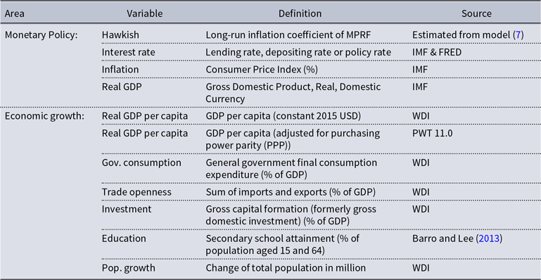
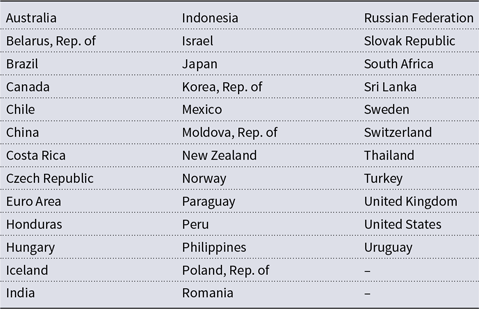
Sample and data. Our sample begins in 2000 and ends in 2020, the close of the most recent five-year block. We include all IT countries listed by Central Bank News (2022) for which sufficiently long time series are available. Most of the data for the growth model come from the World Bank’s World Development Indicators, with the exception of education, for which we use the latest vintage of the dataset originally introduced by Barro and Lee (Reference Barro and Lee2013). Details on variable definitions, transformations, and data sources are provided in Table A.1 and a list of IT countries used in this study in Table A.5 in the Appendix.
3.2 Identification of hawkishness
Our indicators of hawkishness and dovishness are based on a forward-looking specification of the Taylor rule with interest-rate smoothing. The central bank’s desired interest rate
 $r^{*}_{t}$
at time
 $t$
is given by:
 \begin{equation} r^{*}_{t} = b^{*}_{0,t} + b_{1,t}(E_{t}(\pi _{t,K}) - \pi ^{*}_{t}) + b_{2,t} E_{t}(y_{t,K}), \end{equation}
However, in practice the policy rate is typically only gradually adjusted toward the rule-implied rate
 $r^*$
, to avoid financial market volatility, signal policy consistency, and preserve room to avoid hitting the zero lower bound Rudebusch (Reference Rudebusch2002). This yields the policy reaction function,
 \begin{equation} r_{t} = (1 - a_{t}) r^{*}_{t} + a_{t} r_{t-1} + \mu _{t}. \end{equation}
Combining Equation (3) with Equation (4) implies that
 $b_{1,t}$
determines the long-run response of the policy rate to inflation, while the short-run response is
 $(1 - a_t)b_{1,t}$
. Throughout the remainder of the paper, the (policy) response to inflation or inflation coefficient refers to the long-run response
 $b_{1,t}$
.
Rather than imposing an exogenously determined threshold, we classify a country as hawkish at time
 $t$
if its long-run response to inflation,
 $b_{1,t}$
, exceeds the sample median.
Our approach follows Kim and Nelson (Reference Kim and Nelson2006). Their two-step estimation strategy addresses two problems inherent to time-varying forward-looking models.
First, they address endogeneity by rewriting the Taylor rule in terms of future realizations—rather than expectations—and adding a bias-correction term.
When substituting Equation (3) into (4) and replacing expectations with future realizations, we obtain:
 \begin{equation} r_{t} = (1 - a_{t})(b_{0,t} + b_{1,t}\pi _{t,K} + b_{2,t} y_{t,K}) + a_{t} r_{t-1} + e_{t}, \end{equation}
where
 \begin{equation} e_{t} = -(1 - a_{t})[ b_{1,t}(\pi _{t,K} - E_{t}(\pi _{t,K})) + b_{2,t}(y_{t,K} - E_{t}(y_{t,K})) ] + \mu _{t}. \end{equation}
The error term
 $e_t$
is correlated with the regressors
 $\pi _{t,K}$
and
 $y_{t,K}$
by construction, because both enter Expression (6). Recognizing that endogeneity arises from the forecast errors in inflation and the output gap, Kim and Nelson (Reference Kim and Nelson2006) recommend augmenting Equation (5) with orthogonalized prediction errors for
 $\pi _{t,K}$
and
 $y_{t,K}$
generated by an auxiliary model.
This yields the following expression:
 \begin{equation} r_t = (1 - a_t)(b_{0,t} + b_{1,t}\pi _{t,K} + b_{2,t}y_{t,K}) + a_t r_{t-1} + \rho _1\sigma _{e,t} v^*_{1t} + \rho _2\sigma _{e,t} v^*_{2t} + \omega _t, \end{equation}
where
 $v^*_{1t}$
and
 $v^*_{2t}$
are the orthogonalized forecast errors and
 $\omega _t$
is the now independent error term.
Second, although the interest-rate-smoothing parameter generally falls between
 $0$
and
 $1$
in constant-parameter specifications, TVP models can misread increases in the policy rate as explosive dynamics, yielding estimates of
 $a_t$
above one. In this case, the long-run policy coefficients in Equation (5) are no longer well identified
By defining
 $a_t$
as
 \begin{equation} a_t = \frac {1}{1 + \exp ({-}b_{3,t})} \end{equation}
and modeling
 $b_{3,t}$
rather than
 $a_t$
itself as random-walk process addresses this issue.
However, the resulting model is no longer linear. To obtain a tractable representation, Kim and Nelson (Reference Kim and Nelson2006) apply a first-order Taylor expansion to approximate the model linearly. The resulting linear specification, including the bias-correction terms described above, can then be estimated as a TVP model using a standard Kalman filter. In addition to the time-varying Taylor-rule parameters, their model also allows for heteroskedasticity modeled as stochastic volatility.
All Taylor-rules are estimated using quarterly data for the CPI and real GDP, where available, and unemployment otherwise. The data is sourced from the IMF and the Federal Reserve Economic Data FRED, hosted by the Fed St. Louis, and is seasonally adjusted using the X-13 ARIMA-SEATS. The output gap is computed using the Hodrick-Prescott filter. Where possible we use the policy rate, which is otherwise substituted by the lending rate. Where data availability allows, the samples used to estimate Taylor rules start in 1990.
4. Results
4.1 Time-Varying monetary policy reaction function
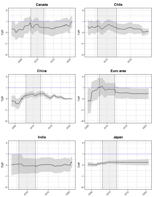
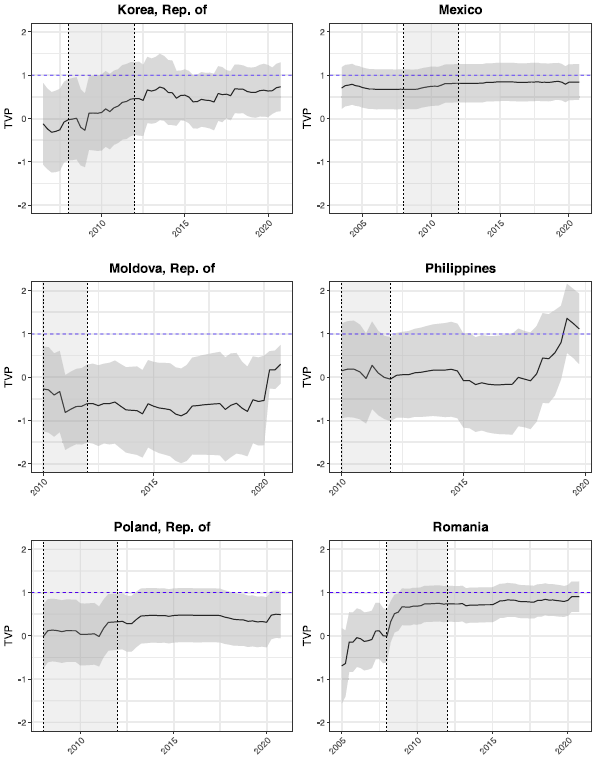
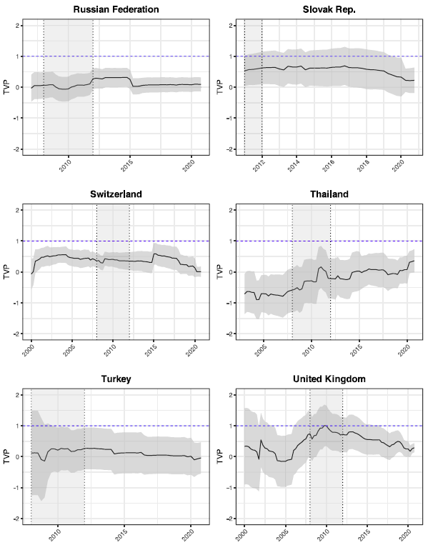
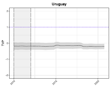
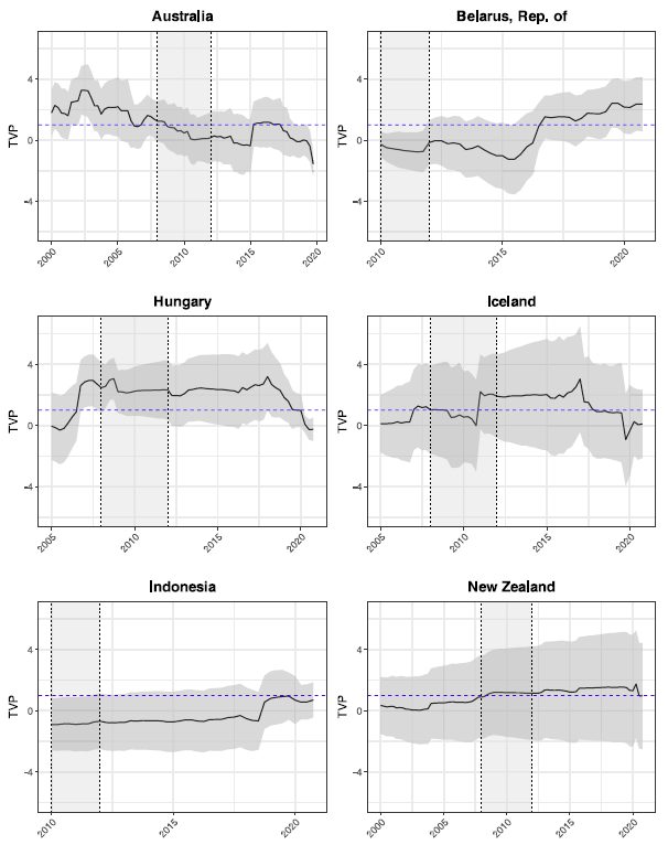
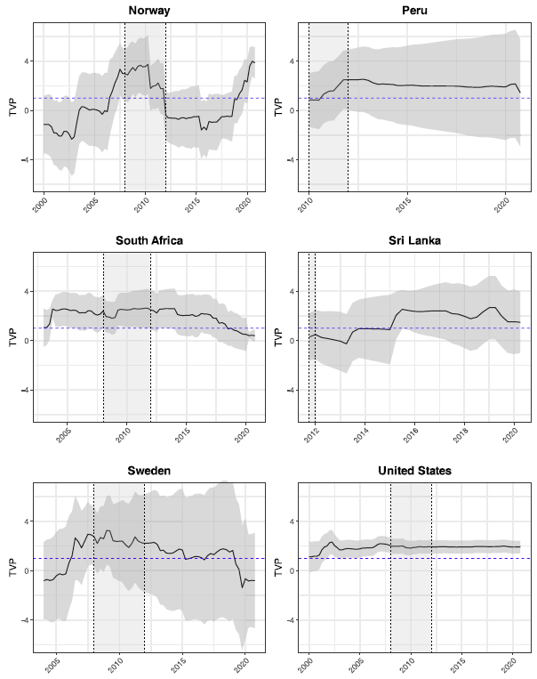
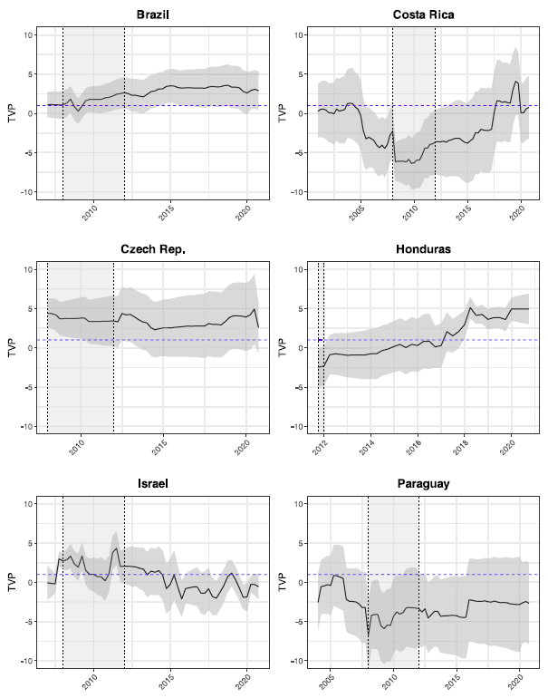
In almost all countries, the long-run response of monetary policy to inflation varies considerably over time (see Figures A.2–A.8).Footnote
2
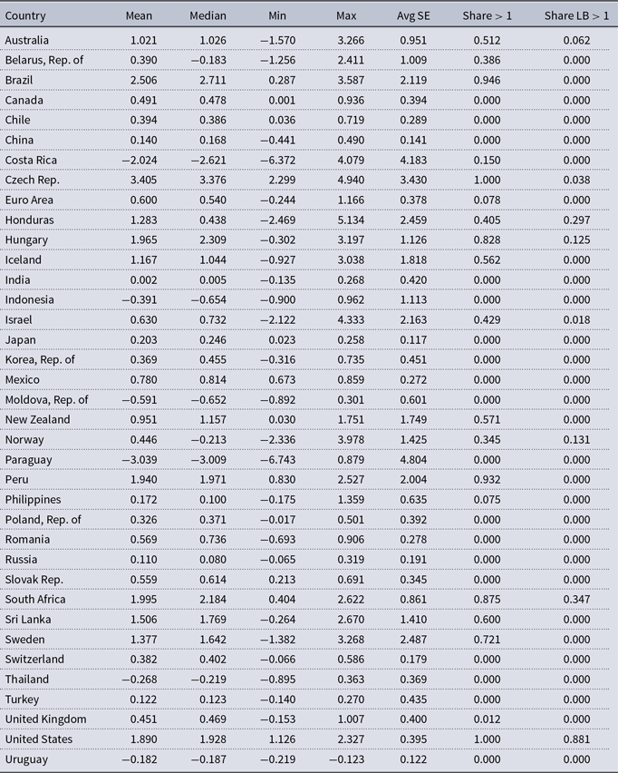
Consistent with earlier evidence (see, e.g., El-Shagi and Ma, Reference El-Shagi and Ma2023), our estimates indicate that the long-run coefficients mostly do not satisfy the Taylor principle. Only in the Czech Republic and the United States do our point estimates exceed one throughout the sample. Eleven additional countries exceed this threshold on average, with New Zealand coming close at a mean of around
 $0.95$
, having maintained a largely above-unity long-run coefficient over the past two decades. In 18 countries,
 $b_{1,t} \leq 1$
throughout the entire sample period—the Taylor principle was consistently not satisfied, see Table A.6.
The exact dynamics differ markedly across countries. While some, such as Costa Rica, India, Israel, Norway, Russia Federation, United Kingdom, and United States exhibit abrupt and sizable shifts, others display more gradual and continuous fluctuations.
The changes are slightly more pronounced during the period surrounding the global financial crisis (2008Q1–2012Q1). In roughly one quarter of the countries in our sample, we observe a considerable decline in the inflation response, suggesting a temporary shift toward greater dovishness. This pattern is consistent with the findings of Anderl and Caporale (Reference Anderl and Caporale2024) and Carvalho and Muinhos (Reference Carvalho and Muinhos2023), who likewise document that central banks tend to prioritize recovery over price stability in the aftermath of crises.
A caveat is that the confidence bounds are very wide for several countries. This reflects a common identification problem: the long-run inflation semi-elasticity of the interest rate is highly sensitive to the choice of smoothing parameter, with even minor adjustments producing substantial variation in the estimated long-run coefficient. To account for this issue, we implement a robustness test in our growth regressions by omitting all countries whose average standard error is above one.
4.2 Effects of key parameters of MPRF on economic growth
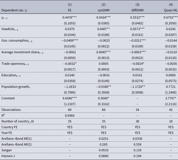
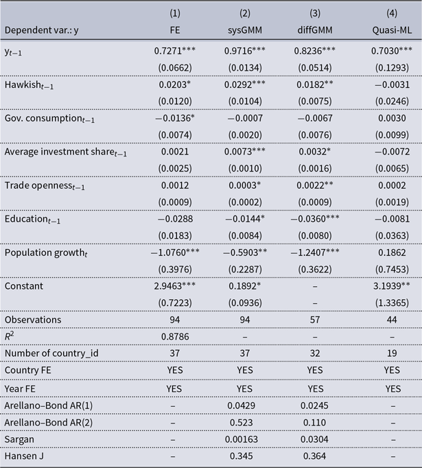
The hawkishness coefficient is positive across all specifications and statistically significant in the system-GMM and difference-GMM estimators, see Table 1. The magnitude is economically meaningful, with estimated coefficients implying growth effects of 4.0 to 5.7 percentage points over a five-year horizon in the GMM specifications. This finding aligns with theoretical contributions (e.g., Gil et al. Reference Gil, Iglésias and Guimaraes2023), which demonstrate that a strong policy reaction to inflation anchors expectations, lowers macroeconomic uncertainty, and promotes investment and long-run growth.
The effects of key parameters of the MPRF on economic growth (PPP-adjusted GDP)

Table 1. Long description
A table comparing the effects of key parameters of the monetary policy reaction function on economic growth using different estimation methods. The table has 11 rows and 5 columns. Column headers are: (1) FE, (2) sysGMM, (3) diffGMM, and (4) Quasi-ML. Row labels are: y_t-1, Hawkish_t-1, Gov. consumption_t-1, Average investment share_t-1, Trade openness_t-1, Education_t-1, Population growth_t, Constant, Observations, R^2, Number of country_id, Country FE, Year FE, Arellano-Bond AR(1), Arellano-Bond AR(2), Sargan, Hansen J. Row 1: y_t-1, 0.4478***, 0.5434***, 0.5532***, 0.6792***. Row 2: Hawkish_t-1, 0.0370, 0.0407**, 0.0573***, 0.0245. Row 3: Gov. consumption_t-1, -0.0409***, -0.0023, -0.0321***, -0.0144. Row 4: Average investment share_t-1, -0.0062, 0.0045**, -0.0063***, -0.0110. Row 5: Trade openness_t-1, -0.0032*, 0.0005, -0.0024*, -0.0036. Row 6: Education_t-1, 0.0140, -0.0031, 0.0161, 0.0869. Row 7: Population growth_t, -1.2633, -0.9180**, -1.1726**, 0.7721. Row 8: Constant, 6.6686***, 0.5660*, 3.7767*. Row 9: Observations, 89, 89, 54, 42. Row 10: R^2, 0.6966, , , . Row 11: Number of country_id, 35, 35, 30, 18. Row 12: Country FE, YES, YES, YES, YES. Row 13: Year FE, YES, YES, YES, YES. Row 14: Arellano-Bond AR(1), , 0.0251, 0.0336, . Row 15: Arellano-Bond AR(2), , 0.285, 0.559, . Row 16: Sargan, , 0.0510, 0.118, . Row 17: Hansen J, , 0.0880, 0.194, .
Note: Standard errors in parentheses. *
*
* p
 $\lt$
0.01, *
* p
 $\lt$
0.05, * p
 $\lt$
0.1. All variables measured in levels (including the hawkish) are end of period values. Lagged values therefore correspond to the value in the reference year of the current growth period. This avoids overlap between policy and its effects. Euro Area and Moldova are excluded from the PPP-adjusted GDP analysis because no PPP-adjusted GDP series exists for either of them.
With respect to the control variables, government consumption and population growth are consistent with standard growth model priors. Both variables have negative coefficients, with population growth statistically significant in the GMM specifications. Given that the model is estimated in levels, the coefficient on lagged GDP captures convergence dynamics documented in earlier work such as Barro et al. (Reference Barro2003), where estimates below unity imply lower growth as income rises, consistent with movement toward the steady state.
4.3 Robustness tests
Removing high uncertainty countries. To ensure that our results are not driven by misclassified countries, we exclude all cases in which the average standard error of the long-run inflation coefficient exceeds unity.
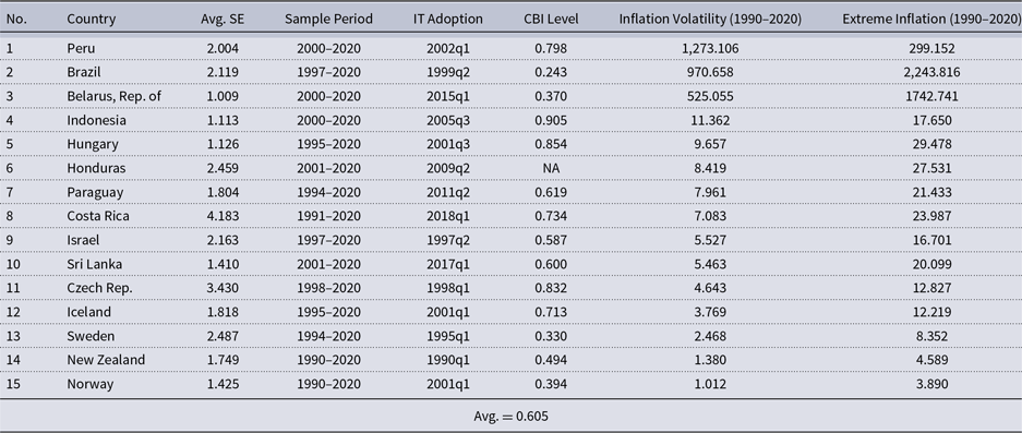
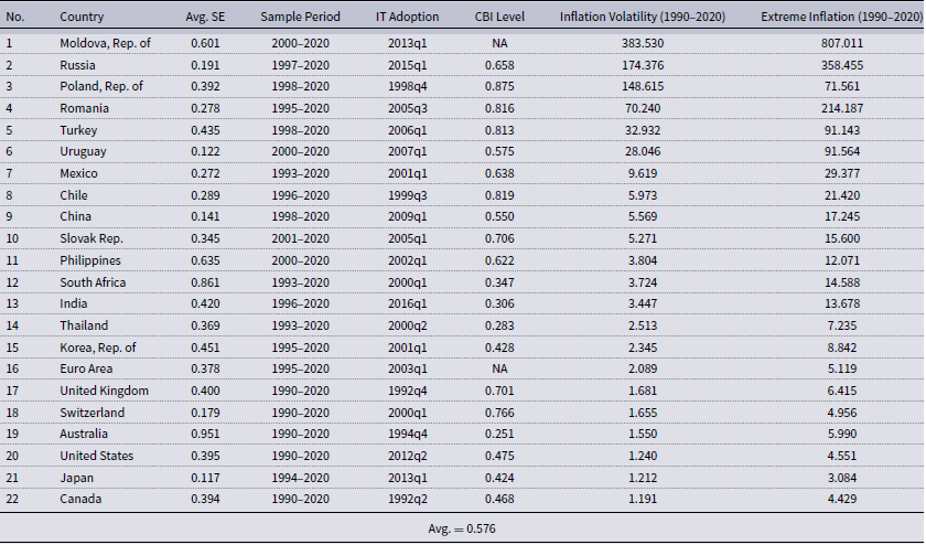
There is no obvious structural similarity setting the high-uncertainty economies apart from the low-uncertainty ones (see Tables A.7 and A.8). Both groups contain countries with hyperinflation episodes and high inflation volatility, a similar distribution of inflation-targeting adoption dates, and a comparable advanced-versus-emerging split. Central bank independence—one of the most widely used predictors of sound monetary policy—does not differ substantially across groups. This restriction therefore appears to reflect estimation precision rather than a shift in the type of economies studied. One caveat remains, high estimation uncertainty may proxy for a greater degree of monetary policy discretion, which could itself be a factor affecting growth. For our objective of studying the impact of policy rules, however, this restriction still is appropriate—it limits the sample to countries that follow the empirical rule more closely and it is thus more meaningful.
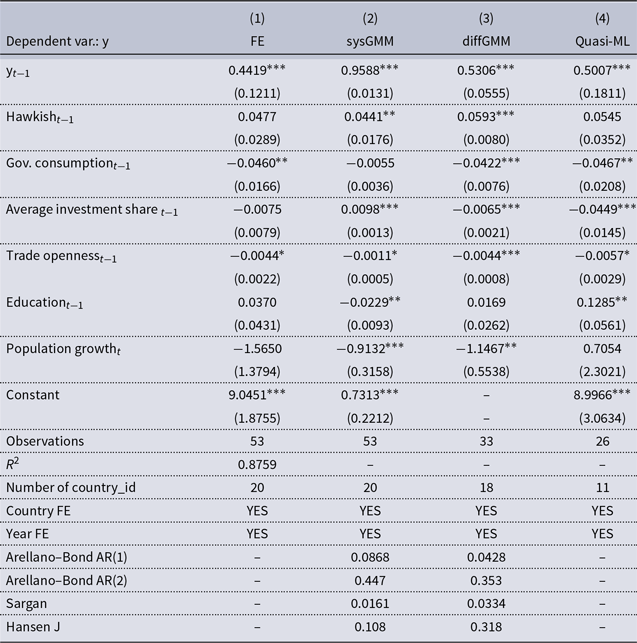
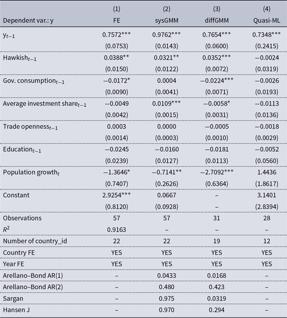
The effects of key parameters of the MPRF on economic growth (Robustness test)

Table 2 Long description
A table with four columns and multiple rows, presenting the effects of key parameters of the monetary policy reaction function (MPRF) on economic growth. The columns are labeled as FE, sysGMM, diffGMM, and Quasi-ML. Each row represents a different variable, including y sub t-1, Hawkish sub t-1, Gov. consumption sub t-1, Average investment share sub t-1, Trade openness sub t-1, Education sub t-1, Population growth sub t, and Constant. Each cell contains a value with standard errors in parentheses and significance levels indicated by asterisks. The table also includes summary statistics such as the number of observations, R-squared values, and various test statistics like Arellano-Bond AR(1), Arellano-Bond AR(2), Sargan, and Hansen J. The table aims to show the robustness of the relationship between these parameters and economic growth across different estimation methods.
Note: Standard errors in parentheses. *
*
* p
 $\lt$
0.01, *
* p
 $\lt$
0.05, * p
 $\lt$
0.1. This sample excludes 15 countries for which the average standard error of the long-run inflation coefficient exceeds unity (see Table A.6). Such cases reflect weakly identified inflation-response parameters – usually from near-unit-root interest rate smoothing or short samples.
The effect of hawkishness on economic growth remains robust after this restriction. GMM estimates range from 4.4 to 5.9 percentage points over a five-year horizon, similar to—and slightly larger than—the baseline. If anything, the effect strengthens when the sample is restricted to countries with more precisely estimated coefficients, suggesting the baseline result is not driven by imprecisely estimated inflation-response parameters (see Table 2). The increase in the estimated growth effect is consistent with low uncertainty reflecting countries with lower discretion—growth effects of the policy rule appear concentrated in economies that follow the rules more closely.
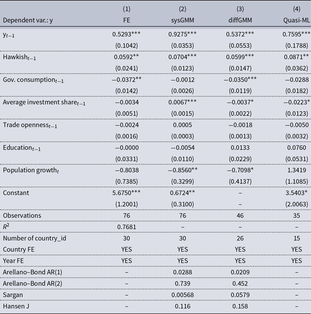
The effects of key parameters of the MPRF on economic growth (PPP-adjusted GDP)

Table 3. Long description
The table presents the effects of key parameters of the monetary policy reaction function on economic growth (PPP-adjusted GDP) using different estimation methods. It includes four columns labeled FE, sysGMM, diffGMM, and Quasi-ML, each representing a different estimation method. The rows are labeled with various parameters and their corresponding coefficients and standard errors. The table has 11 rows and 4 columns. Row 1: Dependent var.: y. Row 2: Yr-1, 0.5293, 0.9275, 0.5372, 0.7595. Row 3: Hawkish1, 0.0592, 0.0704, 0.0599, 0.0871. Row 4: Gov. consumption1, -0.0372, -0.0012, -0.0350, -0.0288. Row 5: Average investment share1, -0.0034, 0.0067, -0.0037, -0.0223. Row 6: Trade openness1, -0.0024, 0.0005, -0.0018, -0.0050. Row 7: Education1, -0.0000, -0.0054, 0.0133, 0.0760. Row 8: Population growth1, -0.8038, -0.8560, -0.7098, 1.3419. Row 9: Constant, 5.6750, 0.6724, -, 3.5403. Row 10: Observations, 76, 76, 46, 35. Row 11: R2, 0.7681, -, -, -. The table also includes additional statistical information such as the number of country IDs, country fixed effects, year fixed effects, and various statistical tests.
Note: Standard errors in parentheses. *
*
* p
 $\lt$
0.01, *
* p
 $\lt$
0.05, * p
 $\lt$
0.1. This sample excludes five countries with highly volatile estimated time-varying long-run inflation coefficients, defined as a standard deviation of first differences exceeding 0.5. These observations are excluded to reduce bias arising from measurement error in the generated regressor. All variables measured in levels (including the hawkish tvp) are end of period values. Lagged values therefore correspond to the value in the reference year of the current growth period. This avoids overlap between policy and its effects.
Excluding countries with highly volatile estimated reaction functions. In several countries,
 $b_{1,t}$
is estimated with comparable precision but fluctuates substantially over time. If the inflation response is not gradually evolving—or at least subject only to relatively rare discrete shifts—the inflation coefficient at the beginning of the corresponding growth period is a poor predictor of the degree of hawkishness throughout that period. Therefore, in a further robustness test we exclude countries with highly volatile estimated policy reaction functions, defined as a standard deviation of
 $\Delta b_{1,t}$
exceeding
 $0.5$
(see Table 3). As with the exclusion of imprecisely estimated countries, this does not alter the qualitative conclusion but somewhat strengthens the estimated effect of hawkishness. In contrast to the baseline, where statistical significance is obtained in two of the four specifications, the coefficient on hawkishness becomes statistically significant across all four estimators, with growth effects ranging from 5.9 to 8.7 percentage points over a five-year horizon.
GDP by PPP vs. GDP in constant USD. Consistent with the broader growth literature, we measure growth using PPP-adjusted real GDP as the baseline outcome. At the same time, studies on the growth effects of central bank characteristics, such as inflation targeting and central bank independence, often use GDP in constant U.S. dollars. Replacing PPP-adjusted GDP with GDP in constant U.S. dollars therefore serves as a robustness check and leads to moderate changes in the estimates. The coefficients are somewhat smaller than in the baseline, while the positive effect remains statistically significant in three of the four estimators, compared with two in the PPP-based baseline (see Table A.2).
Applying the same robustness checks using GDP in constant U.S. dollars yields smaller coefficient magnitudes relative to the PPP-based results. When restricting the sample to observations with well-identified inflation semi-elasticities, the implied growth effects range from 3.2 to 3.8 percentage points (Table A.3). When, in addition, highly volatile central banks are excluded, the effects decline further to between 2.0 and 3.2 percentage points (Table A.4). In both cases, the coefficients remain positive and statistically significant in three specifications, while the quasi–maximum-likelihood estimates are small and not statistically significant.
5. Conclusion
We analyze the relationship between the long-run inflation semi-elasticity of the policy rate and economic growth using data from 37 IT countries. Our findings indicate sizable and statistically robust effects of a more hawkish policy stance—measured as an above-median inflation semi-elasticity—on economic growth, with annual impacts ranging from 0.8% to 1.7% across specifications.
Whereas the previous literature has largely focused on the growth effects of inflation targeting—typically interpreted as an official commitment to a stated inflation target—our results suggest that adopting the label alone may be insufficient. This underscores that even under monetary frameworks widely viewed as best practice, the time-inconsistency problem can still bias policymakers toward short-run stabilization at the cost of long-run growth.
This points to new directions for the literature on central bank institutions and growth: rather than examining individual institutional features and their interactions with external factors such as development or governance quality, it may be necessary to assess how different dimensions of monetary policy jointly interact. For example, the lack of emphasis on inflation—even within an inflation-targeting framework—may well be linked to insufficient central bank independence.
Appendix A
Scatter plot of hawkishness against interest rates.

Time-varying long-run response of the policy rate to inflation, with 90% confidence bands.

Table 2 Long description
A table with four columns and multiple rows, presenting the effects of key parameters of the monetary policy reaction function (MPRF) on economic growth. The columns are labeled as FE, sysGMM, diffGMM, and Quasi-ML. Each row represents a different variable, including y sub t-1, Hawkish sub t-1, Gov. consumption sub t-1, Average investment share sub t-1, Trade openness sub t-1, Education sub t-1, Population growth sub t, and Constant. Each cell contains a value with standard errors in parentheses and significance levels indicated by asterisks. The table also includes summary statistics such as the number of observations, R-squared values, and various test statistics like Arellano-Bond AR(1), Arellano-Bond AR(2), Sargan, and Hansen J. The table aims to show the robustness of the relationship between these parameters and economic growth across different estimation methods.
Time-varying long-run response of the policy rate to inflation, with 90% confidence bands.

Time-varying long-run response of the policy rate to inflation, with 90% confidence bands.

Time-varying long-run response of the policy rate to inflation, with 90% confidence bands.

Time-varying long-run response of the policy rate to inflation, with 90% confidence bands.

Time-varying long-run response of the policy rate to inflation, with 90% confidence bands.

Time-varying long-run response of the policy rate to inflation, with 67% confidence bands.

Definition and sources of the variables used

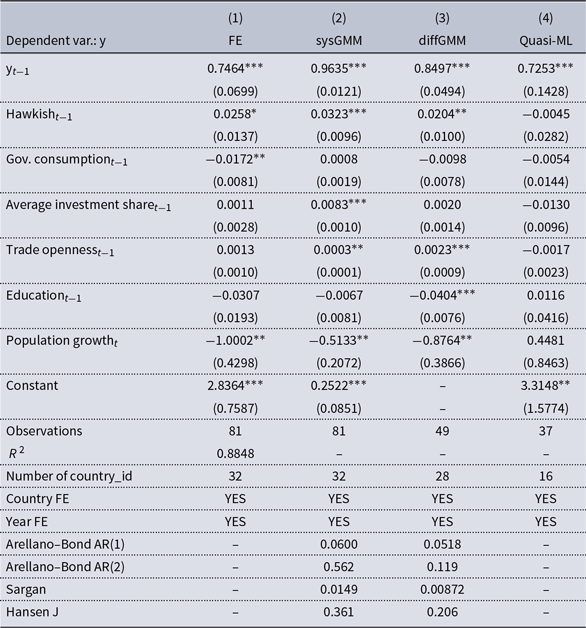
The effects of key parameters of the MPRF on economic growth

Table A2. Long description
A table comparing economic growth using different estimators and variables. The table has 11 rows and 5 columns. Column headers are: (1) FE, (2) sysGMM, (3) diffGMM, and (4) Quasi-ML. Row labels include: Dependent var.: y, y_t-1, Hawkish_t-1, Gov. consumption_t-1, Average investment share_t-1, Trade openness_t-1, Education_t-1, Population growth_t, Constant, Observations, R^2, Number of country_id, Country FE, Year FE, Arellano-Bond AR(1), Arellano-Bond AR(2), Sargan, Hansen J. Row 1: Dependent var.: y. Row 2: y_t-1, 0.7572***, (0.0753), 0.9762***, (0.0143), 0.7654***, (0.0600), 0.7348***, (0.2415). Row 3: Hawkish_t-1, 0.0388**, (0.0150), 0.0312**, (0.0122), 0.0352***, (0.0072), -0.0024, (0.0319). Row 4: Gov. consumption_t-1, -0.0172*, (0.0090), 0.0004, (0.0041), -0.0224***, (0.0071), -0.0026, (0.0193). Row 5: Average investment share_t-1, -0.0049, (0.0042), 0.0109***, (0.0015), -0.0058*, (0.0031), -0.0113, (0.0136). Row 6: Trade openness_t-1, 0.0003, (0.0014), 0.0000, (0.0003), -0.0005, (0.0010), -0.0018, (0.0029). Row 7: Education_t-1, -0.0245, (0.0239), -0.0160, (0.0127), -0.0181, (0.0113), -0.0052, (0.0560). Row 8: Population growth_t, -1.3646*, (0.7407), -0.7141*, (0.2626), -2.7092***, (0.6364), 1.4436, (1.8617). Row 9: Constant, 2.9254***, (0.8120), 0.0667, (0.0928), -, -, 3.1401, (2.8394). Row 10: Observations, 57, 57, 31, 28. Row 11: R^2, 0.9163, -, -, -. Row 12: Number of country_id, 22, 22, 19, 12. Row 13: Country FE, YES, YES, YES, YES. Row 14: Year FE, YES, YES, YES, YES. Row 15: Arellano-Bond AR(1), -, 0.0433, 0.0168, -. Row 16: Arellano-Bond AR(2), -, 0.480, 0.423, -. Row 17: Sargan, -, 0.975, 0.0319, -. Row 18: Hansen J, -, 0.970, 0.294, -.
Note: Standard errors in parentheses. *
*
* p
 $\lt$
0.01, *
* p
 $\lt$
0.05, * p
 $\lt$
0.1. All variables measured in levels (including the hawkish) are end of period values. Lagged values therefore correspond to the value in the reference year of the current growth period. This avoids overlap between policy and its effects.
The effects of key parameters of the MPRF on economic growth (Robustness test)

Note: Standard errors in parentheses. *
*
* p
 $\lt$
0.01, *
* p
 $\lt$
0.05, * p
 $\lt$
0.1. This sample excludes 15 countries for which the average standard error of the long-run inflation coefficient exceeds unity (see Table A.6). Such cases reflect weakly identified inflation-response parameters – usually from near-unit-root interest rate smoothing or short samples. All variables measured in levels (including the hawkish) are end of period values. Lagged values therefore correspond to the value in the reference year of the current growth period. This avoids overlap between policy and its effects.
The effects of key parameters of MPRF on growth (constant-USD GDP)

Note: Standard errors in parentheses. *
*
* p
 $\lt$
0.01, *
* p
 $\lt$
0.05, * p
 $\lt$
0.1. This sample excludes five countries with highly volatile estimated time-varying long-run inflation coefficients, defined as a standard deviation of first differences exceeding 0.5. These observations are excluded to reduce bias arising from measurement error in the generated regressor. All variables measured in levels (including the hawkish tvp) are end of period values. Lagged values therefore correspond to the value in the reference year of the current growth period. This avoids overlap between policy and its effects.
List of inflation-targeting countries

Summary statistics of time-varying inflation-response coefficient (
 $b_{1,t}$
)

Notes: The table reports summary statistics of the time-varying inflation-response coefficient (
 $b_{1,t}$
) from the estimated Taylor rule. “Share
 $\gt 1$
” denotes the fraction of observations for which
 $b_{1,t} \gt 1$
. “Share LB
 $\gt 1$
” denotes the fraction of observations for which the lower bound of the 90% confidence interval exceeds one.
Countries with high uncertainty

Countries with low uncertainty

 b1,t