


1. Introduction
The 1920s were characterized by the rapid expansion in credit in many countries, particularly during the second half of the decade, after monetary stabilization had proceeded in most European countries and international capital flows had resumed (Eichencreen and Mitchener, Reference Eichengreen and Mitchener2004; Schularick and Taylor, Reference Schularick and Taylor2012; Accominotti and Eichencreen, Reference Accominotti and Eichencreen2016). Country-specific studies have used individual bank balance sheet data to study the nature and causes of the 1920s credit booms, emphasizing the role of credit expansion and bank vulnerability in predicting subsequent bank distress in the United States and Germany (Postel-Vinay, Reference Postel-Vinay2016, Reference Postel-Vinay and Schularick2022; Postel-Vinay and Collet, Reference Postel-Vinay and Collet2024), Italy (Battilossi, Reference Battilossi2009; Molteni, Reference Molteni2024a, Reference Molteni2024b), or France (Baubeau et al., Reference Baubeau, Monnet, Riva and Uncaro2021). This paper studies the causes of the bank lending boom of the late 1920s in Spain, which coincided with the rapid deterioration of the exchange rate of the peseta. Bank lending boomed between 1927 and the banking crisis of 1931, averaging a 10% increase per quarter, year-on-year (Table 1). During the same period, current account and fiscal deficits widened, and the Spanish peseta began to fall rapidly (Figure 1).Footnote 1 While the depreciation of the peseta during the late 1920s brought some benefits—mainly stemming from the evolution of domestic prices with respect to international prices—it was not a deliberate policy choice (Ecuidazu, Reference Ecuidazu1979; Martín-Aceña, Reference Martín-Aceña1984; Martínez-Ruiz and Nocués-Marco, Reference Martínez-Ruiz and Nogués-Marco2014; Barbaroux et al., Reference Barbaroux, Jorge-Sotelo and Torre2026). Spanish policymakers decried the fall of the peseta and sought to prevent it, but why did their efforts fail?
Bank lending growth and exchange rate depreciation, 1924–1934.

Figure 1 Long description
The x-axis represents time from 1924 quarter 1 to 1934 quarter 4. The left y-axis shows year-on-year growth in bank loans, ranging from negative 0.2 to 0.2. The right y-axis shows pesetas per pound, ranging from 30 to 50. A bar graph represents bank loans, with fluctuations visible, peaking around 1931 quarter 1. A line graph represents pesetas per pound, showing a decline from 1927 quarter 1, reaching a low around 1931 quarter 1 and then slightly rising towards 1934 quarter 4.
Bank lending boom episodes by type of banks and boom threshold

Table 1 Long description
The table examines bank lending boom episodes across different types of banks and boom thresholds, measured by average year-over-year growth. At a 0.5 standard deviation threshold, all banks experienced a boom from late 1926 to late 1930, with an average growth of 10.80%. CSB Top 6 banks consistently showed higher growth rates across all thresholds, peaking at 11.68% at 1.5 standard deviations. Non-CSB banks did not experience a boom and showed negative growth at higher thresholds, indicating a lack of lending activity. The data suggests that larger CSB banks were more resilient during boom periods compared to smaller or non-CSB banks. Interpretation should consider the varying periods and growth rates across different bank groups and thresholds.
Note: When no bank lending boom is identified, the average YoY growth is calculated for the same period as the full sample of banks (All).
This article argues that the answer lies in the effects of banking reform, as evidenced by the passage of the 1921 Banking Law. The law institutionalized a system of indirect government debt monetization by banks at subsidized rates, which ensured strong demand for government debt and provided a liquidity safety net for most banks, on which they relied to expand their balance sheets during the boom. This law also changed the operational framework of Banco de España (BdE, henceforth), and granted it with a new, safer stream of revenue through lending on collateral, rather than relying on the outright purchase of commercial securities. As a result, money creation by banks and therefore the evolution of aggregate credit—especially any attempt to curb it—was subordinated to the needs of the fiscal authorities (Comín, Reference Comín2012; Comín and Cuevas, Reference Comín and Cuevas2017). This mechanism of indirect debt monetization by the banking system has been discussed previously at the aggregate macroeconomic level, and recent quantitative approaches using time-series analysis have focused on its implications for the evolution of aggregate monetary magnitudes. These works conclude that there was a regime of “fiscal dominance” in the long run (1874–1998) (Sabaté et al., Reference Sabaté, Gadea and Escario2006, Reference Sabaté, Gadea and Escario2015). In turn, both contemporary observers and recent researchers discussed its origins and functioning (Paret, Reference Paret1921; Comisión del Patrón Oro, 1929; Olariaca, Reference Olariaga1946; Pedrós Abelló, Reference Pedrós Abelló1978; Martín-Aceña, Reference Martín-Aceña1984; Comín, Reference Comín1988; Martínez Mendez, Reference Martínez Mendez2005).
Previous research has argued that the role of this “indirect debt monetization” mechanism has been exaggerated by contemporaries and scholars, both in terms of its role in bank lending and its impact on the exchange rate. One argument of this view is that, during the 1920s, the resort to this mechanism was relatively timid. In particular, it is argued that it was only relevant in macroeconomic terms after the Spanish Civil War, from 1939 to 1959, when it was finally abolished as part of the 1959 Stabilization Plan. However, while it is true that the Francoist regime resorted to this mechanism at an unprecedented scale, this does not imply that it had no role to play in the bank lending boom during the Primo de Rivera Dictatorship during the late 1920s, particularly considering that Spain had a much more open capital account in the 1920s than in the 1940s and 1950s and that during the late 1920s—a period of volatile capital flows—fiscal and monetary dynamics were reflected in the evolution of the exchange rate. A second argument raised by this view is that banks have always used this mechanism well below the maximum limits established by the BdE (Martín-Aceña, Reference Martín-Aceña1984; Martínez Mendez, Reference Martínez Mendez2005).
This paper provides evidence for a contrasting view. I argue that in order to ensure that banks remained liquid in the event of a banking crisis, the 1921 Banking Law created an automatic contingent liability at the BdE on which banks relied when expanding their balance sheets between 1927 and 1931. As I document below, for the indirect debt monetization mechanism to influence bank lending, banks did not necessarily need to draw on their credit accounts with the BdE; they simply ensured that their public debt portfolios were accepted by the BdE for potential, contingent liquidity needs. So far, despite the points outlined above, the role of banks has not been empirically documented, even though this was the fundamental mechanism through which indirect debt monetization was expected to affect credit creation. To shed light on the mechanisms by which indirect debt monetization operated, I exploit a newly collected and digitized quarterly database on disaggregated bank balance sheets that includes all banks operating in Spain between 1922q4 and 1934q4. Details on the different items of both assets and liabilities allow exploration of the channels through which monetary policy changes affected bank lending (or did not), depending on portfolio composition.
The 1921 Banking Law established the Consejo Superior Bancario (CSB), an embryonic regulatory body to which banks could voluntarily join if they met specified requirements. This divided the Spanish banking system between CSB members and nonmembers. Because of this division, the database I create allows for an estimation of the differential reaction to the changes in BdE interest rates for the two types of banks after controlling for a number of bank characteristics and dynamics of the real economy. I follow the standard literature on the transmission of monetary policy through bank loans and find that the more banks could rely on the liquidity backstop provided by the BdE on government bonds, the less reactive they were to changes in the monetary policy stance. This confirms contemporaries’ concerns that the 1921 Banking Law worked as a fiscal backstop for present and future governments, as well as to increase the interaction between the BdE and the rest of the banking sector, and contributed to the modernization of the money market, but that the monetization mechanism it created clashed with the aims of curbing exchange rate depreciation. Moreover, this mechanism of “indirect monetization” of persistent fiscal deficits through banks’ credit creation was an important driver of total bank lending, and thus had substantial macroeconomic consequences.
Information on the dating of the bank lending boom is presented in Table 1, which confirms the intuition presented in Figure 1. To identify and date this episode, I aggregate the quarterly stock of bank loans over the available period, 1922q4 to 1934q4. I calculate these aggregates for five categories of banks: all banks, CSB member banks, the top 6 CSB member banks, CSB member banks excluding the top 6, and non-CSB member banks. I define a bank lending boom as a period when the cyclical component of bank lending growth exceeded a threshold of k standard deviations above zero and when the actual growth rate of bank lending was positive.Footnote 2 I report these episodes using different thresholds to allow for sensitivity. Focusing on CSB banks, the results in Table 1 indicate a lending boom beginning by the beginning of 1927 and ending between 1929q4 and 1931q1, depending on the threshold. Importantly, results also show that nonmember banks did not experience a lending boom, with an average growth in bank loans much smaller than for CSB member banks.
The rest of the paper is organized as follows. Section 2 discusses the 1921 Banking Law and its implications. Section 3 describes the empirical approach and the data sources. Section 4 provides the results, and a discussion of the context, and Section 5 concludes.
2. The 1921 Banking Law
Amid the state’s growing fiscal needs, the BdE charter was renewed in 1891 in exchange for a 150 million peseta loan.Footnote 3 Its monopoly of issuance was set to last for 30 years, only to be renewed before the end of 1921. Monetary stability and strong fiscal restraint characterized the early 20th century, as Spain recovered from the macroeconomic effects of its defeat in the Cuban War (Comín, Reference Comín2012; Eichencreen and Esteves, Reference Eichengreen and Esteves2022). From 1914, however, and due to Spain’s neutrality during World War I, external demand for Spanish goods boomed as European belligerent countries reallocated resources and demanded imports. After decades of deficit, the Spanish trade balance moved into a large surplus, which peaked in 1919. The armistice precipitated the collapse of Spanish exports, which began to fall in 1920 and continued to decline in 1921. In turn, imports boomed in 1920, as pent-up demand for foreign products began to be satisfied, particularly amid the strong exchange rate appreciation of the war years. Despite imports declining after the postwar surge, trade deficits persisted throughout the 1920s (Tena, Reference Tena, Carreras and Tafunell2005). Alongside the real expansion of the economy, the banking sector had also experienced rapid growth. Banks had expanded their regional networks during and after the War, and several new institutions had been founded (Martín-Aceña, Reference Martín-Aceña1984, Reference Martín-Aceña and Economico2005; Tortella and Palafox, Reference Tortella and Palafox1984). Banks contributed to financing the war boom by expanding their supply of financial services and by developing a network of branches throughout the country (Paris Ecuilaz, Reference Paris Ecuilaz1947; Velarde, Reference Velarde1968; Martín-Aceña, Reference Martín-Aceña1984; Pueyo, Reference Pueyo2006). The expansion of the banking sector brought about a change in the composition of the money supply, and
monetary authorities lost a large part of the direct control they had over the money supply until then. If monetary authorities wanted to regulate the money market, they had to take care not only of their own consolidated balance sheet, but to exert a tighter control over the evolution of the liabilities of the banking sector. (Martín-Aceña, Reference Martín-Aceña1985, p. 17)
Before the charter was due for renewal, the post-war crisis brought about a large bank failure in Spain. In December 1920, Banco de Barcelona (the oldest non-issuing bank in Spain at the time) failed. The bank had undergone a strong expansion during wartime in order to take advantage of the economic boom in Spain, as well as to compete with foreign banks that established branches in Spain during the same years. The collapse of foreign demand, international commodity prices, and foreign exchange volatility, along with internal mismanagement, caused the bank to fail (Blasco and Sudrià, Reference Blasco and Sudrià2016). Some prominent members of the executive argued that the failure had been caused by a panic unrelated to the bank’s fundamental health, and pushed for the view that the bank would have survived if it had received more assistance from the BdE or the government.Footnote 4 Leading this debate was Mr. Francesc Cambó, who was appointed Minister of Finance in August 1921. While Cambó acknowledged the mismanagement problems within the bank’s organization and their role in the bank’s failure, as well as the role of the international commodity price collapse.Footnote 5 However, he stressed the importance of improving banks’ access to a liquidity backstop during periods of financial distress and to a more elastic currency during normal times, thereby marking what is considered the first step towards turning the BdE into a lender of last resort (Martín Aceña, Reference Martín-Aceña2017). Although the BdE had acted as lender of last resort before, it had enjoyed a considerable degree of discretion (Jorge-Sotelo, Reference Jorge-Sotelo2019, Reference Jorge-Sotelo2020, Reference Jorge-Sotelo2025). This discretion was, according to Mr. Cambó, the product of a fragmented banking system in which the central bank was disconnected from and competed with the rest of the banking system, so regulating banks’ access to central bank liquidity was seen as a priority to avoid liquidity crises in the future. Paraphrasing the 1913 Congressional mandate of the Federal Reserve to provide with an “elastic currency,” he argued that “in a credit system, the issuing bank has to be the rearguard, a very firm position that is not subject to convulsions, keeping always the necessary firmness to be able to assist the banks, which in turn need a higher elasticity to be able to attend the needs and changing nature of the nation’s economic life”.Footnote 6
2.1. The content of the law
The 1921 Banking Law—which went by as the Cambó Law—was strongly shaped by the 1920 banking crisis, and as such, one of its aims was to deepen money market modernization (Jorge-Sotelo, Reference Jorge-Sotelo2022). The 1921 Banking Law was passed on December 29, 1921, 2 days before the monopoly of issuing expired. The Law had two parts. The first addressed the BdE, while the second addressed the rest of the banking system through the creation of the CSB, a regulatory body to which banks could voluntarily adhere, provided they were admitted. In this subsection, first, I discuss the impact of the law on the BdE, and second, the creation of the CSB and its impact on the rest of the banking system.
2.1.1. Banco de España (BdE)
The law addressed several questions concerning the BdE. Here, I discuss Sections 7 and 8 of Article 1, which are the most relevant for the argument.Footnote 7 Section 7 dealt with the eventual need to intervene in foreign exchange markets to stabilize the peseta. This section contemplated not a systematic intervention in foreign exchange markets to stabilize the peseta, but rather an eventual need to intervene. Therefore, the law did not include any commitment from the BdE or the government to control exchange rate fluctuations. Instead, it was stated that if the foreign exchange situation required a stabilization intervention, the government would have to take the initiative. If the BdE agreed to the government’s stabilization plans, it could contribute to them with its own resources (its gold reserve). The intervention would be financed 50% by the government, and 50% by the BdE, and any profits or losses resulting from the intervention would be shared accordingly.Footnote 8 This reflected the extent of the BdE’s bargaining power during the law’s negotiation. With this clause, BdE avoided the eventual internalization of a time-inconsistency problem: a future government could pursue fiscal policy incompatible with a stable exchange rate, forcing BdE to embark on a stabilization program with an uncertain outcome, risking its gold reserves and profits. Hence, the law provided that if government debt followed a path the BdE considered inconsistent with exchange rate stability (as in the second half of the 1920s), the BdE could simply decline any proposal for a stabilization plan. However, no specific metric was defined; neither on what was considered exchange rate stability nor on how much fiscal deficit was acceptable. In practice, therefore, exchange rate management fell into a void in which no specific institution was given a specific mandate about it (Martín-Aceña, Reference Martín-Aceña1984; Martínez-Ruiz and Nocués-Marco, Reference Martínez-Ruiz and Nogués-Marco2014), despite underlying aspirations of exchange rate stabilization and eventual adhesion to the interwar gold exchange standard (Jorge-Sotelo, Reference Jorge-Sotelo2020; Barbaroux et al., Reference Barbaroux, Jorge-Sotelo and Torre2026).
Section 8 introduced a reduction in the discount rate (the interest rate at which BdE would conduct outright purchases of 90-day commercial bills of exchange) and in the Lombard rate on public debt (the rate BdE would charge for 3-month advanced credit—or advances—secured by government bonds). This reduction would be only enjoyed by CSB member banks when borrowing from BdE.Footnote 9 Although a reduction in the discount rate had been contemplated by a law drafted in 1918, this was optional for the BdE, and it was not introduced as compulsory until the 1921 Banking Law.Footnote 10 An important nuance of Section 8 was that, while the decision to rediscount a bill of exchange was ultimately at the discretion of the BdE, its assessment of the quality of the signatures presented,Footnote 11 the latter could not reject CSB member banks’ Lombard operations using public debt as collateral. As in other countries in Europe during the 1920s (Eichencreen, Reference Eichengreen1992), this was part of the modernization of the money market aimed by the law, as it implied that once the Law was passed, the BdE would be ready to interact with all CSB members, at least, through Lombard loans against public debt.Footnote 12
The discount rate on the outright purchase of commercial bills of exchange charged to CSB members was reduced by 1.0% vis-à-vis other private clients (including nonmember banks and foreign banks, provided that their signature was eligible), unless the official rate was below 5.0%, in which case the reduction was of 0.2%.Footnote 13 This bonus aimed at progressively withdrawing BdE from the private discount business by providing the public with an incentive to discount bills with banks. Advances against public debt were also granted a reduction. This one, however, was not constant and predetermined. The Law opened the possibility for different Lombard rates applying to different types of government bonds (and also to private stocks). The Lombard rate on government bonds could be set by the BdE, the CSB, and the Minister of Finance whenever a new issuance of public debt occurred. This meant that, while there was a standard rate for advances against public debt, if the government needed to issue more debt than the market was willing to accept, it could avoid paying higher yields by setting a specific lower rate for advances. Importantly, this type of operation differed from modern-day repurchase operations (repo) in that the bank in question did not sell the bonds to the BdE, as the latter was forbidden to buy them both in the primary and the secondary market. This specific part of Section 8 was highly controversial, as it reflected the underlying time-inconsistency: the rate at which CSB banks could monetize their public debt holdings at the BdE was already below the nominal yield of government bonds but, in addition, this rate could be further lowered for specific issuance if needed by future governments. A heated parliamentary debate on the potential consequences of this mechanism for exchange rate and price stability took place, with propositions to limit the ability of the government to set Lombard rates, but the final text contemplated that a specific Lombard rate for new issuance of public debt could be renegotiated between banks (CSB), the BdE, and the government at any given moment.Footnote 14
The process of government debt monetization was not necessarily automatic in the sense that it did not need to take place immediately after the government issued new debt.Footnote 15 When banks purchased public debt in the primary or secondary market, they could keep it in their balance sheet while prepositioning it at BdE for an eventual liquidity need.Footnote 16 Thus, purchasing government bonds resulted in an earning asset, while prepositioning these bonds at BdE resulted in a costless liability for banks, which was reflected in their balance sheets as “deposits in banks and bankers” (Depósitos en bancos y banqueros). In turn, the total amount of government bonds that banks prepositioned at the BdE defined the maximum amount the BdE would be willing to convert into cash upon request by banks (reflected as máximo disponible in the BdE accounts). After netting out the interbank assets, the resulting interbank liabilities reflect this process (Martínez Mendez, Reference Martínez Mendez2005, Annex 29, p. 11). This is depicted in Figure 2a, which shows the average increase in the share of deposits at BdE held by banks relative to their total peseta deposits. It also shows how, as soon as concerns emerged about the evolution of the peseta and excessive liquidity in the money market in 1928, banks began to preposition government bonds with BdE to ensure these would be ready to draw upon. Banks prepositioned around 500 million pesetas in government bonds at BdE (Figure 2b). This was immediately reflected in banks’ cash reserves held at BdE, which is reflected in Figure 2c, where I plot the evolution of banks’ cash reserves as a share of total assets. As can be seen, in the same moment as banks prepositioned the bonds, their cash reserves almost doubled, from averaging 6% of total assets to almost 12%. As explained by Gorton et al. (Reference Gorton, Ross and Ross2025), this mechanism improved contingent liquidity conditions for most banks and provided them with a reliable safety net to which they could access without incurring a net cost.Footnote 17 However, it also increased their ability to issue a loan and create a concomitant deposit without necessarily using and paying for the Lombard facility, unless they were under liquidity pressure to do so. In sum, Section 8 in Article 1 of the 1921 Banking Law provided banks with a remunerated liquidity safety net, regardless of whether they ended up drawing upon it or not.
Banks’ prepositioning of government debt (1925q1–1934q4).

Figure 2 Long description
The image A shows a line graph titled 'Bank deposits at BdE' with the x-axis labeled with quarterly dates from 1925 to 1934 and the y-axis labeled 'Bank deposits at BdE as percentage of deposits'. The graph shows a trend with a notable increase after the 'First Discount Rate change' marked in 1928 quarter 4. The image B shows a graph titled 'CSB interbank assets and liabilities' with the x-axis labeled with quarterly dates from 1925 to 1934 and the y-axis labeled 'Deposits at BdE and interbank assets in thousand pesetas'. It features two lines: one for interbank assets and another for bank deposits at BdE, both showing an upward trend after the 'First Discount Rate increase' in 1928 quarter 4. The image C shows a line graph titled 'Cash reserves' with the x-axis labeled with quarterly dates from 1925 to 1934 and the y-axis labeled 'Cash reserves as percentage of assets'. The graph indicates a sharp increase in cash reserves following the 'First Discount Rate Change' in 1928 quarter 4, followed by fluctuations over the subsequent years.
2.1.2. CSB member and nonmember banks
Article 2 of the 1921 Banking Law created a new institutional and regulatory framework for banks: the Consejo Superior Bancario (CSB; Supreme Banking Council in English). CSB membership was voluntary, so there was selection into membership. All banks in Spain, including CSB members, nonmembers, and foreign banks, had to fill out harmonized quarterly balance sheet data and send it to CSB. On the asset side, CSB members had to comply with liquidity and leverage ratios and could not underprice the BdE by discounting bills in the market below its discount rate. On the liability side, the CSB introduced ceilings on interest paid on deposits for different maturities. As per the motivation of the Law, the goal of the CSB was to set a uniform regulatory criterion for banking, so banks would be under the same discipline, and fragmentation and the occurrence of large outlier situations like Banco de Barcelona in 1920 would be avoided in the future. Contemporary observers soon highlightedFootnote 18 that the establishment of the CSB as a group of banks, subject to certain regulations, which were granted access to the central bank’s discount window, mirrored the 1913 Federal Reserve Act (Mitchener and Richardson, Reference Mitchener and Richardson2013; Calomiris et al., Reference Calomiris, Jaremski, Park and Richardson2015). In fact, after World War I, the US government introduced a system in which member banks could borrow from the Federal Reserve using government bonds (Liberty bonds) at rates below their nominal yields (Meltzer, Reference Meltzer2003).
The Ministry of Finance appointed the President of the CSB (Comisario Regio). The rest of the board members were appointed as follows: one by the BdE, six in representation of the different regional banking interests—Centre (A), Northwest (B), and Northeast (C)—and one appointed by the Chamber of Industry, Trade and Shipping.Footnote 19 Six of the nine members thus came from the banking sector and were directors of some of the largest Spanish banks at the time.Footnote 20 The board of CSB stipulated minimum liquidity and capital ratios.Footnote 21 The liquidity rule stipulated that CSB banks had to maintain a two-thirds ratio between their short-term liquid assets (activo realizable) and their short-term liabilities (pasivo exigible). Liquid assets, under the CSB definition, included: cash and deposits at the BdE, foreign exchange in cash, interbank loans, 3-month bills of exchange, public debt (at 90% of their value), stocks (at 80% of their value), collateralized loans, call loans, and loans in foreign exchange (Footnote 21). In short, everything except long-term (uncollateralized) loans was included in the liquidity ratio, meaning that this measure was very lax and not binding, which is not surprising after considering that more than two-thirds of the body that decided on these regulatory measures was filled with direct representatives of the banking interests. In turn, short-term liabilities included: call deposits (current accounts), deposits in foreign exchange, interbank deposits, and the share of time deposits that could be withdrawn with less than 8 days’ notice. Capital ratios were also defined.Footnote 22 Paid-in capital, reserves, and 50% of the non-paid-in capital had to be above 10% of the banks’ deposits. If, for exceptional circumstances, banks exceeded the liquidity and capital ratio limits, they had to submit the case to the CSB for evaluation, which would consider whether a penalty applied. However, as Artola-Blanco (Reference Artola-Blanco and Faboulet2016) highlighted, the liquidity rule was discussed only internally within CSB and was never officially published, so it is very likely that it was never enforced; the bank-level evidence presented here suggests that it was far from binding. A similar dilution of the effective binding capacity of these ratios was observed in Italy during the same period (Molteni and Pellecrino, Reference Molteni and Pellegrino2024).
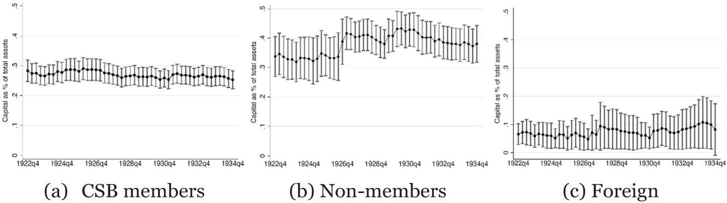
Figure 3 shows the evolution of the liquidity ratios established by the CSB for member, nonmember, and foreign banks compared to the minimum limit (indicated by the horizontal line at 2/3). Given the laxity of the liquidity rule, it is not surprising that both CSB members and nonmembers held similar ratios (Figure 3a and b). Foreign banks presented a different picture, mostly driven by their higher proportion of deposits in foreign exchange with respect to the other two types of short-term liabilities computed in the ratio (sight deposits, interbank deposits, and less than 8-day deposits) (Figure 3c). A similar picture emerges when comparing banks’ capital ratios. Given the data at hand, which does not allow for distinguishing between paid and unpaid-in capital, it is not possible to calculate the CSB-determined capital ratios for all banks. However, an approximation can be done by comparing a standard capital ratio, which includes capital and reserves as a percentage of total assets (Figure 4). Again, there seems to be no positive relation between CSB membership and capital ratios. Rather, the contrary, nonmembers held higher capital ratios than CSB members (Figure 4a and b). Although CSB members had very high capital ratios—in the vicinity of 30% of assets—compared to other countries,Footnote 23 the difference between both groups makes sense if we consider that nonmembers had no access to the facilities that the 1921 Banking Law established for member banks when accessing the discount window of the BdE and the fact that they were, on average, much smaller banks.Footnote 24
Average and minimum liquidity ratios established by CSB, 1922–1934.

Figure 3 Long description
The image consists of three line graphs comparing liquidity ratios defined by CSB for different bank categories from 1922 to 1934. The first graph (a) shows CSB members with liquidity ratios fluctuating around 2.5. The second graph (b) depicts non-members with more variability, peaking above 3.0. The third graph (c) illustrates foreign banks with ratios generally below 2.5. All graphs include a horizontal line indicating the CSB liquidity ratio limit at 2 over 3. The x-axis is labeled with quarterly intervals from 1922q4 to 1934q4 and the y-axis is labeled 'Liquidity ratio defined by CSB' ranging from 0.5 to 3.5.
Average capital ratios, 1922–1934.

Figure 4 Long description
The image consists of three line graphs labeled (a), (b) and (c). Graph (a) shows the capital as a percentage of total assets for CSB members from 1922 to 1934. The x-axis is labeled with years from 1922 to 1934 and the y-axis is labeled 'Capital as percentage of total assets'. The graph shows a relatively stable trend with slight fluctuations. Graph (b) represents non-members, showing more variation with peaks and troughs over the same period. Graph (c) depicts foreign banks, showing an increase in capital percentage towards the end of the period. Each graph includes error bars indicating variability in the data points.
Being a CSB member carried a number of substantial benefits outlined above and had a very small cost, reflected in very lax regulatory requirements that were not effectively binding. This raises the question of why some banks did not join CSB. Banks could join CSB at any time after its creation, provided they were accepted, and could withdraw as well. While there is no systematic evidence on acceptance and refusal of membership, some cases were discussed by the CSB board. In most cases, the main reason for admission or rejection was that the bank in question “did (or did not) perform genuine banking activities.”Footnote 25 It is difficult to determine exactly what this meant, and the minutes of the CSB Admissions Board (Junta de Admisiones) are not available, to the best of my knowledge. However, a plausible explanation is that the reason some banks were not accepted at CSB is that they held noncommercial bills of exchange (so-called financial or accommodation bills), which were considered at the time to be inflationary because they did not stem from a genuine commercial transaction in which real goods were involved, as per the “real bills doctrine.”Footnote 26 In the empirical analysis below, CSB membership is not treated as a treatment in the experimental or causal sense, but rather as a defining characteristic of banks that may affect the transmission of monetary policy. In particular, the main characteristic of nonmembers is that they could not “earmark” bonds and borrow from BdE at subsidized rates. This implies that self-selection is not expected to pose a problem in interpreting the results.
2.1.3. Timing of the law and its impact on the money market
As Comín and Cuevas (Reference Comín and Cuevas2017) argue, the law changed the role of BdE,
from a direct financier of the State to a broker for private banks in negotiating the issues and subscriptions of public debt (…). As investing in public debt was profitable for private banks, their growth bolstered their demands for a greater involvement in this business. This combined well with the willingness of the Ministers of Finance to broaden their financial bases, taking full advantage of the growing strength of the resources of private banks, directly negotiating the debt issues with these entities.Footnote 27
While the outcome of the law benefited all parties, it created conflicts with other policy objectives, such as exchange rate stability, which contemporaries openly decried in parliamentary debates.Footnote 28
The outcome of the law was strongly influenced by timing; the monopoly of issuance of BdE had to be renewed before December 31, 1921, and the shocks caused by the war boom, the postwar crisis, and the 1920 banking crisis determined different parties’ bargaining power. First, and foremost, the fiscal needs of the Spanish state rose sharply during 1921. The government debt-to-GDP ratio had been falling steadily and rapidly since the turn of the century, due to strong fiscal adjustment and subsequent primary surpluses, from 120% of GDP to 45%. However, by 1920, fiscal deficits grew to around 45% of expenditures, following the end of the war boom, and public debt as % of GDP rose rapidly again, to 60% in 1 year (Comín and Diaz, Reference Comín, Diaz, Carrreras and Tafunell2005a). The impact of the postwar economic collapse on the fiscal accounts was further exacerbated by the so-called Disaster of Annual, amid the ongoing war in the Spanish dominions in Morocco (Comín, Reference Comín2012). Military defeat became a possibility after this episode, and a sudden large-scale military deployment required placing a substantial amount of public debt in the market over a short period, amid a worsening economic situation (Figure 5), so demand for government bonds had to be secured. Since BdE could not buy public debt in either the primary or the secondary market, the law had to find a way to satisfy the government’s financial needs through the banking sector. By introducing public debt as a security that BdE could not reject as collateral and by being able to jointly determine its Lombard rate, this new mechanism allowed for the monetization of public debt without the latter showing up in the balance sheet of the BdE as such, but rather as credit to commercial banks. In other words, the 1921 Banking Law discharged the BdE from directly monetizing public debt by outsourcing it to non-issuing banks (Martín-Aceña and Martínez Ruiz, Reference Martín-Aceña and Martínez Ruiz2022). As contemporary observers put itFootnote 29:
(…) Nowadays, the debts of the State are not a burden to the Banco [BdE], instead, the State places the bondholder [the CSB bank participating in the primary market] between the Treasury and the Banco. Discount policy is managed in such a way that the bondholder finds an immediate and direct profit in subscribing to the bonds, as it can borrow from the Banco. The creation of credit is then in favour of the bondholder; the Banco’s balance sheet is not inflated with public debt; now it is private instead of public debt, what fills the gap that in previous times was filled by the debts of the Treasury.
Public and private stocks issued, 1903–1933.

Figure 5 Long description
A bar graph showing the total issued per year in million pesetas from 1903 to 1933. The x-axis represents the years from 1903 to 1933, while the y-axis shows the total issued per year in million pesetas, ranging from 0 to 2,500. Two types of bars are present: public debt and private stocks. Public debt is represented by black bars and private stocks by gray bars. Notable peaks in public debt issuance occur in 1918, 1921 and 1922, with the highest peak in 1922. Private stocks show smaller fluctuations throughout the years, with moderate increases in the early 1920s and late 1920s.
During parliamentary debates about the law, despite the government’s allusions to the urgency to pass the law because of the expiration of the monopoly of issuance, several members of the opposition argued that the state could leave the BdE charter in suspension in order to get more time to debate the law and find a solution to deem the discount rate effective without subordinating exchange rate stability to the path of fiscal deficits.Footnote 30 Moreover, growing financial instability during the autumn of 1921 added to the time pressure. Almost a year after the failure of Banco de Barcelona, banks in the same city faced renewed liquidity pressure as they incurred losses on foreign exchange positions, with some banks suffering large losses.Footnote 31 This added pressure to the government to reach an agreement on how emergency liquidity ought to be provided and how to ensure that Spanish banks could count on the “elastic currency” to which Mr. Cambó alluded. Pressure mounted for the government to ensure that an agreement was reached with BdE regarding liquidity provision against a homogeneous type of collateral, with a clear market price, and that ensured minimum liquidity buffers for banks. Yet criticism arose because the law created incentives for banks, BdE, and the government that compromised exchange rate stability if fiscal imbalance continued to grow in the futureFootnote 32:
Our Banking Law clearly states that the State intervenes in the determination of the discount rate and the rate charged on advances against public debt. (…) It is a condition to the stabilisation of our exchange rate that the production of public debt ceases (…).
The law had an immediate impact on the Spanish money market and introduced a regime change in how monetary policy was implemented in Spain (Jorge-Sotelo, Reference Jorge-Sotelo2022). First, it altered the operational framework of the BdE and its balance sheet, making it an outlier among interwar central banks. Immediately after the law’s enactment, the bulk of BdE’s lending would be conducted through Lombard loans on public debt, while rediscounting would assume a secondary role. Figure 6a shows the ratio between Lombard loans (advances) and discounts at the BdE, with the former outpacing the latter right after the passage of the law.Footnote 33 In turn, from 1921, the share of profits accruing to private shareholders of BdE came from Lombard operations involving government debt (Figure 6b). As a result, Spain became the only major European country in which Lombard loans replaced rediscounting as the central bank’s main money-market instrument (Table 2), despite open-market operations on government debt gradually becoming the main monetary policy instrument during the interwar period (Eichencreen, Reference Eichengreen1992). While BdE had been reluctant to give “great latitude” to these operations before the passing of the 1921 Banking Law, after that, these became the central bank’s preferred monetary policy instrument.Footnote 34
Changes in BdE lending operations and profits (1900–1935).

Figure 6 Long description
The image contains two graphs. The first graph, labeled 'Evolution of BdE lending portfolio', has the x-axis labeled 'Year' from 1900 to 1935 and the y-axis labeled 'Ratio Advances / Discounts'. It shows a fluctuating trend with a notable increase after the 1921 Banking Law, peaking around 1925 before declining. The second graph, labeled 'Composition of BdE profits', has the x-axis labeled 'Year' from 1900 to 1935 and the y-axis labeled 'BdE profits (thousand pesetas)'. It displays two lines: one for 'Discount' and another for 'Advances'. Both lines show an increase after the 1921 Banking Law, with 'Advances' peaking higher than 'Discounts' around 1925, followed by a decline. The 1921 Banking Law is marked on both graphs with a vertical line.
Central banks’ portfolio composition, 1880–1928

Table 2 Long description
The table compares the portfolio composition of central banks across various countries from 1880 to 1928, focusing on advances/discounts and public debt/securities ratios. Britain shows a significant increase in public debt/securities from 38% in 1880 to 60% in 1928, with advances/discounts peaking at 1.0 in 1928. Austria's advances/discounts remained low, while its public debt/securities decreased from 14% to 8%. Spain's advances/discounts rose sharply to 2.5 in 1928, with a notable drop in public debt/securities from 61% to 6%. Greece and Bulgaria had high public debt/securities ratios in 1928, at 97% and 70% respectively. The data reflects varied financial strategies and economic conditions across countries, with some figures representing averages or adjusted years due to anomalies or data availability.
Source: Jobst and Ucolini (Reference Jobst and Ugolini2016) for data from Austria to Switzerland (the figure for Britain is the average ratio for 1875–1885, as advances behave abnormally during some years and cause ratios that do not reflect the common practice of the Bank of England at the time). Leacue of Nations (1925–1937) for data from Denmark to Yugoslavia (1913 instead of 1909). Martínez Mendez (Reference Martínez Mendez2005) for Spain (data are for 1900 instead of 1882).
Second, it created strong incentives for CSB member banks to hold large shares of public debt in their portfolios. Figure 7 shows the significant difference between public debt as a percentage of the securities portfolio for CSB members and nonmembers. During the 1920s, particularly during the last quarter of 1927, banks’ holdings of public debt started increasing much faster than their holdings of commercial bills (Figure 8a). This was facilitated by the debt conversion that took place in 1927–1928 (Figure 8b) and the large debt issue in 1928 and 1929 (Figure 5). In the first months of 1927, the government started the conversion of 5,225 million pesetas from short-term floating debt into long term 5% redeemable bonds; by the end of the year, the conversion had been successfully completed, with banks ending up holding most of the newly issued consolidated bonds (Martín-Aceña and Comín, Reference Martín-Aceña and Comín1984). The conditions of the conversion explain why banks engaged in this conversion strongly, considering how this debt could then be monetized at the BdE. They were offered two options: either a conversion to 85.5% of par, or at 98% with fiscal exemption of the prevailing 20% tax on public debt interest earnings (Comín, Reference Comín1988; Pan-Montojo, Reference Pan-Montojo, Álvarez Nogal and Comín Comín2015). Both cases represented an attractive option for banks, given that it increased their ability to borrow from the BdE and, by that time, the Lombard rate for these bonds was set at 4%. Importantly, as Figure 9 shows, CSB member banks enjoyed a positive spread between the average yield-to-maturity (YTM) of government bonds and the Lombard rate during the whole period, while non-CSB members didn’t. The risk of government default in the short run was largely absent, as the debt conversion made clear, so the large spike in government bond yields registered in 1931 was primarily due to exchange rate risk as capital flight ensued during the 1931 financial crisis.Footnote 35
Public debt as % of portfolio of securities.

Figure 7 Long description
The image contains two line graphs. The first graph, labeled (a) CSB members, shows public debt as a percentage of securities from 1922 quarter 4 to 1934 quarter 4. The y-axis represents public debt as a percentage of securities, ranging from 0 to 0.5. The x-axis shows time in quarters from 1922 quarter 4 to 1934 quarter 4. The data points fluctuate around 0.4 with error bars indicating variability. The second graph, labeled (b) Non-members, also shows public debt as a percentage of securities over the same period. The y-axis and x-axis are similarly labeled. The data points for non-members fluctuate around 0.3, with error bars indicating variability. Both graphs illustrate trends and variations in public debt as a percentage of securities over time for the two groups.
Composition of bank portfolios and public debt (1922–1935).

Figure 8 Long description
The image contains two line graphs. The first graph, labeled '90 day bills and public debt', has the x-axis labeled with quarters from 1922 quarter 4 to 1934 quarter 4 and the y-axis labeled 'Total bank portfolios (thousand pesetas)'. It shows two lines: one for '3m bills of exchange' and another for 'Public debt'. The 'Public debt' line shows a general upward trend, while the '3m bills of exchange' line fluctuates. The second graph, labeled 'Public debt in circulation', has the x-axis labeled from 1922 to 1935 and the y-axis labeled 'Public debt (million pesetas)'. It shows three lines: 'Treasury (short-term)', 'State (long-term)' and 'Total'. All lines show an upward trend, with 'Total' being the highest, followed by 'State (long-term)' and 'Treasury (short-term)'.
Government debt yields and BdE policy rates, 1920s–1930s.

Figure 9 Long description
The image contains two graphs. The first graph (a) shows BdE rates and public debt yield to maturity (YTM) from January 1920 to January 1936. The y-axis represents BdE rates and public debt yields in percentage. Multiple lines represent different years: 1900, 1917, 1926, 1927, 1929 and Lombard rates for gold bonds, average and discount. The second graph (b) illustrates the spread between public debt YTM and the BdE Lombard rate on public debt from the fourth quarter of 1922 to the fourth quarter of 1934. The y-axis shows the spread value. Two lines represent CSB members and non-members, with CSB members generally having a higher spread than non-members, especially around 1930 to 1932.
The 1921 Banking Law worked to define the collateral framework on which Spanish money markets would develop during the interwar period, but it became subject to the contradiction between the Spanish authorities’ goal of exchange rate stability and the ability of banks and the government to indirectly monetize public debt with the BdE. As shown in Figure 1, bank lending grew at an average annual rate of 10% per quarter (year-on-year) between 1927 and the 1931 crisis, while the external value of the peseta fell rapidly during the same period. As the depreciation of the peseta became the government’s main economic concern from early 1928, the framework established by the 1921 Banking Law revealed its pro-cyclical nature. In a scenario of fiscal and current account deficits and the tightening of international financial markets, the government needed to issue new debt to fund its growing expenditures and borrow to stabilize the exchange rate. The strategy, however, was always going to be self-defeating had it not been coupled with an improvement in fiscal accounts.
3. Empirical strategy
In order to test whether the changes introduced by the 1921 Banking Law had effects on the transmission of monetary policy in Spain, this section outlines the empirical approach and the data sources used.
3.1. Dynamic panel data model on bank lending
I estimate a loan equation derived from the monetary policy transmission model proposed by Ehrmann, Gambacorta, Martínez-Pages, Patrick, and Worms (2003), which captures the impact of changes in policy rates on bank lending. This model is chosen because it allows for interactions between the monetary policy indicator and different bank characteristics, in order to capture the asymmetries in the transmission of monetary policy depending on these characteristics. The estimated loan equation is the following:
 \begin{align}
\Delta {\text{In}}\,\text{(}Loan{s_{it}}\text{)} & = {a_i} + \sum\limits_{j = 1}^l {{b_j}\Delta {\text{In}}\,{\text{(}}Loan{s_{it - j}}{\text{)}}}\nonumber\\
&\quad + \sum\limits_{j = 0}^l {{c_j}\Delta \,{\text{Monetary}}{\text{Polic}}{{\text{y}}_{{{t - j}}}} + } \sum\limits_{j = 0}^l {{d_j}\Delta {\text{In}}\,{\text{(}}GD{P_{t - j}}{\text{)}}}\nonumber\\
&\quad + \sum\limits_{j = 0}^l {{e_j}CP{I_{t - j}} + fCharacteristi{c_{it - 1}}}\nonumber\\
& \quad + \sum\limits_{j = 0}^l {{g_{1j}}Characteristi{c_{it - 1}}} \cdot \Delta \,MonetaryPolic{y_{t - j}}\nonumber\\
& \quad + \,hControl{s_{it}} + \,{\varepsilon _{it}}
\end{align}
where i = 1, …, N, N the number of banks and t = 1, …, T with T the number of quarters. For the first term on the right-hand side of the equation, j is the number of lags of the dependent variable (log of loans in pesetas) included in the estimation, and accordingly, Loansit is the end-of-quarter loan portfolio of bank i in period t (lending to corporates and families). The model is estimated with four lags of the dependent variable to capture seasonality within a year. To capture the effects of the 1921 Banking Law on the transmission of monetary policy, I use different indicators for this variable: Discount and Lombard rates for CSB members, the YTM of public debt, and the spread between the latter and the Lombard rate (see below). Economic output and prices are captured in GDPt and CPIt, respectively. Bank-specific characteristics (size, liquidity and capital ratios, and CSB membership) are captured by the vector xit and, as explained above, they are interacted with the monetary policy variable. I include a number of controls in the regression: the Madrid stock market index, an index of the exchange rate of the peseta, foreign central banks’ discount rates, and a banking crisis dummy for the 1931 crisis.Footnote 36 As in all standard estimations in the literature, the model allows for fixed effects (Anceloni et al., Reference Anceloni, Kashyap and Mojon2003; Gambacorta and Marques-Ibañez, Reference Gambacorta and Marques-Ibañez2011).
If central bank rates are effective in reducing bank lending, one would then expect the coefficient associated with MonetaryPolicyt −j to be negative (see Table A6 in the appendix for a summary of main estimates in the literature). In the original model presented by Ehrmann et al. (Reference Ehrmann, Gambacorta, Martínez-Paces, Patrick, Worms, Angeloni, Kashyap and Mojon2003), banks have to reduce leverage because their reserves become insufficient after the central bank absorbs them through open market sales that raise market rates. In my case, monetary policy (rate changes) can be ineffective because it does not lead to a reduction in base money; continued deficits and their monetization kept the monetary base increasing regardless of BdE rate changes. In the case at hand, however, this may not have occurred because CSB banks had no incentive to reduce leverage when the BdE raised rates. Their reserves were unchanged precisely because they could continue to pledge public debt to the BdE.
There are two challenges when estimating Equation 1. The first one is that in order to allow for dynamics, the model has to include the lagged value of the dependent variable. The introduction of dynamics in the panel estimation needs to be taken into consideration, as the error term can be correlated with past realizations of the dependent variable, introducing endogeneity. The second is that in order to disentangle the effect of changes in monetary policy from other macroeconomic variables, the model needs to include measures of real output, inflation, stock market index, exchange rate, etc. All these measures—mostly but not only real output—complicate causal inference from the estimation, as business cycle dynamics are expected to be a major determinant of demand for loans. This poses a problem because we aim to isolate the effect of monetary policy on the dependent variable, which is the bank loan supply.
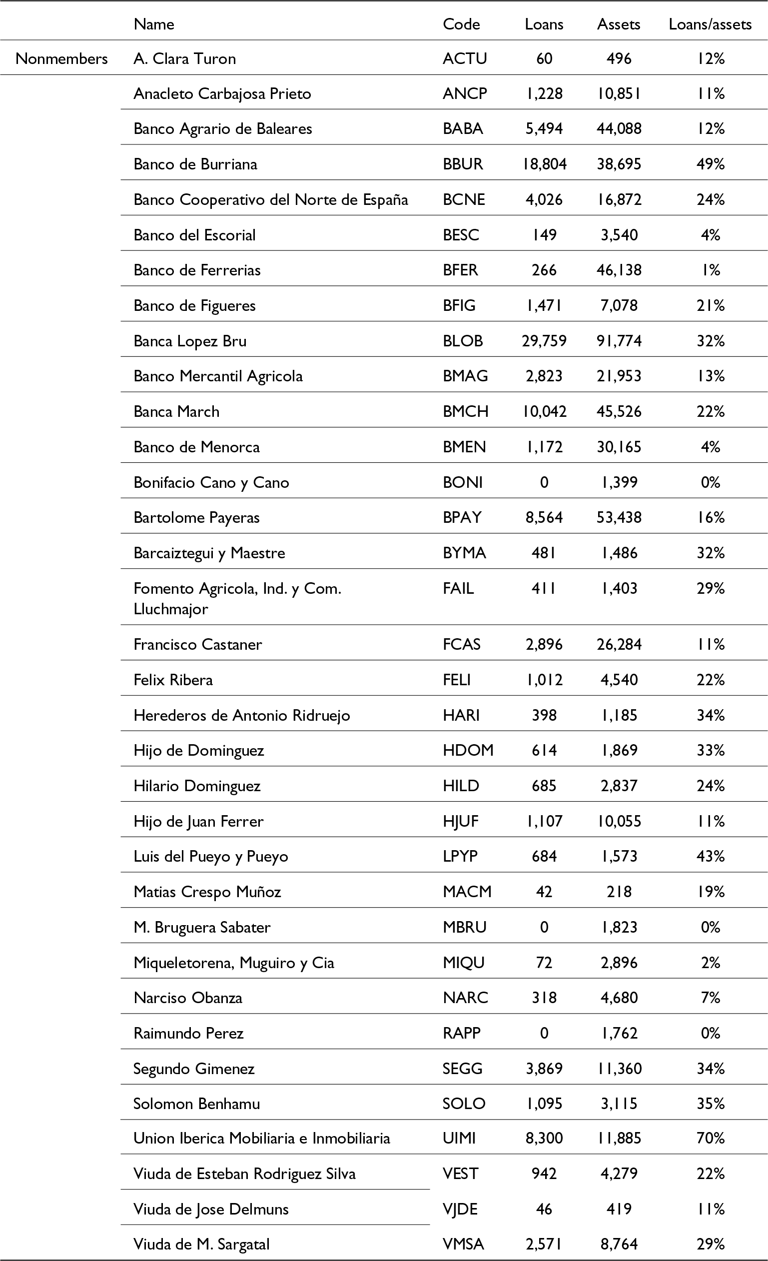
The literature interested in identifying the transmission of monetary policy has traditionally dealt with these two challenges by implementing the difference GMM (generalized method of moments) estimator developed by Arellano and Bond (Reference Arellano and Bond1991), which provides with efficient and consistent estimators, provided that the instruments are chosen to take into account the serial correlation properties of the model.Footnote 37 Dynamic-panel estimation with GMM is, in fact, indicated for panels in which T is relatively small and N is relatively large. Therefore, and in order to have a balanced panel, I limit the analysis to the period that maximizes the number of bank-quarter observations while still including the crucial years of 1927–1931. The final sample leaves me with a balanced panel that comprises 130 banks over 23 quarters (1927q1–1932q3), so a total of 2990 bank-quarter observations. From this, 96 are CSB members, while 34 are nonmembers. Foreign banks (11 banks) are excluded from the estimation.Footnote 38
3.2. Data
3.2.1. Bank balance sheets and bank characteristics
Starting in the last quarter of 1922, both members and nonmembers of the CSB submitted their harmonized balance sheets, and the CSB published and distributed them afterward. This dataset has been used partially in previous research (Jorge-Sotelo, Reference Jorge-Sotelo2020), but this is the first attempt at exploiting quarterly bank balance sheet item-level data on the universe of Spanish banks. A brief discussion of the new database is presented in the appendix. I collect these data from the Boletines del CSB, which contain quarterly observations on various asset and liability items from 1922q4 to 1934q4. Not only do CSB member banks appear in the database, but also nonmembers and foreign banks, as they were also obliged to report their balance sheets.Footnote 39 The resulting sample comprises quarterly balance sheets for 302 banks from 1922q4 to 1934q4, for a total of 49 time periods. Observations are at the end of the period. However, I limit the sample to 130 banks for the 1927q1–1932q3 period. This captures all the changes in the BdE rate and, more importantly, the surge in bank lending that started in 1927. In the appendix, additional estimates are conducted using a wider time span (1926q1–1933q4) to enhance robustness (Tables A4 and A5).
To estimate Equation 1, I aggregate three types of bank loans: call loans, loans on collateral, and long-term loans (see the appendix for details on balance sheet items). All loans are in pesetas. I use other items on the balance sheet to construct liquidity and capital ratios (see below). Following the standard literature in the transmission of monetary policy, I include three bank characteristics:Footnote 40 size, capital ratios, and liquidity ratios.Footnote 41 Bank size is calculated as the log of total assets. Capitalization is the ratio of capital and reserves over total assets. Finally, liquidity is computed as the ratio of liquid assets (90-day bills of exchange and public debt) over total assets. In addition, I include the main characteristic of interest, which is CSB membership. Membership takes the value 1 for nonmember banks and 0 for CSB member banks, in order to easily interpret the coefficients in the estimations below. The interaction between membership and monetary policy indicator captures the differential reaction of nonmember banks to changes in monetary policy. Membership is also interacted with the other characteristics (size, capital ratios, and liquidity ratios). As stated above, to a large extent, banks selected themselves into being CSB members, so this interaction should not be interpreted as a random assignment of a treatment but rather for comparative purposes regarding monetary policy transmission, in the same way as banks holding higher or lower capital or liquidity ratios are also not exogenous bank characteristics but a strategic decision taken by banks.Footnote 42 In this sense, while the relationship between monetary policy changes and bank lending should be interpreted as causal and mediated by bank balance sheet characteristics, CSB membership should not. Precisely because banks self-select into CSB membership and this directly influences their balance sheet characteristics relative to nonmember banks, CSB membership should not be interpreted as a treatment but rather as an additional characteristic that limits banks’ direct access to central bank liquidity.
Overall, CSB banks’ assets account for approximately 95% of total assets during the period, while nonmembers account for the remaining 5% (excluding foreign banks). These proportions are stable throughout the period. Table 3 presents descriptive statistics for the main variables concerning bank balance sheets, separated by CSB membership and for two subsamples: one including all banks and another excluding the six largest banks (all CSB members). I provide the mean, the standard deviation, and the p-value for a t-test on the means of CSB vis-à-vis No-CSB banks. There are some important differences in the structure of the two groups’ balance sheets. First, in terms of their securities’ portfolio, CSB members held less 90-day bills of exchange and more public debt and private stock. The fact that CSB members held around twice as much public debt as nonmembers is not surprising, given the superior eligibility of this type of security at the discount window of the BdE. Second, CSB member banks operated with significantly lower equity ratios, consistent with their ready access to a liquidity backstop.Footnote 43 However, the fact that nonmembers held a larger share of 90-day bills of exchange is not intuitive at first, because if these bills were eligible at the discount window of the BdE, then it would mean nonmembers were losing out on the 50-basis points reduction in the rediscount rate that CSB members enjoyed, and thus it would not make sense for them to remain outside CSB. While we lack information on the exact types of bills in banks’ portfolios, this difference may be due to the requirement that bills sold to BdE reflect a genuine commercial transaction (under the so-called real bills doctrine). The very large share of bills in nonmembers’ portfolios might reflect that they held a different type of bill, so-called financial bills, which were ineligible.
Descriptive statistics

Table 3 Long description
The table presents descriptive statistics comparing financial metrics between CSB and No-CSB groups, including cash, securities, and debt ratios. Key findings include significant differences in 90-day bills/securities and public debt metrics, with No-CSB showing higher means in these categories. The p-values for these differences are statistically significant, suggesting a meaningful distinction between the groups. The data also highlights that No-CSB has a higher capital-to-assets ratio compared to CSB. The mean values are unweighted averages, and the interpretation should consider the variability indicated by standard deviations.
Note: Mean is the unweighted average. Source: See text
3.2.2. Monetary policy indicators
The monetary policy indicator is the primary variable of interest. Following the contemporary discussion on the inability of the BdE to control aggregate lending that took place during the parliamentary debate on the 1921 Banking Law, I use the two main rates of the BdE: the discount rate and the Lombard rate as monetary policy indicators.Footnote 44 Both are used, including the reduction in CSB banks’ exposure. Data on interest rates is taken from Martínez Mendez (Reference Martínez Mendez2005). Interest rates are introduced at their end-of-quarter values. In addition to official rates, I use two additional indicators of monetary conditions: the YTM on public debt and the spread between the latter and the Lombard rate (see Figure 9b). These last two indicators are expected to capture the channel through which Spanish monetary authorities lost control of the evolution of aggregate credit following the 1921 Banking Law. Given the move towards restrictive monetary policy that started in early 1928 in the United States and Germany, in all specifications of the model, I include the reference interest rate of foreign central banks (Bank of England, Federal Reserve, Banque de France, and Reichsbank).Footnote 45
3.2.3. Macroeconomic variables
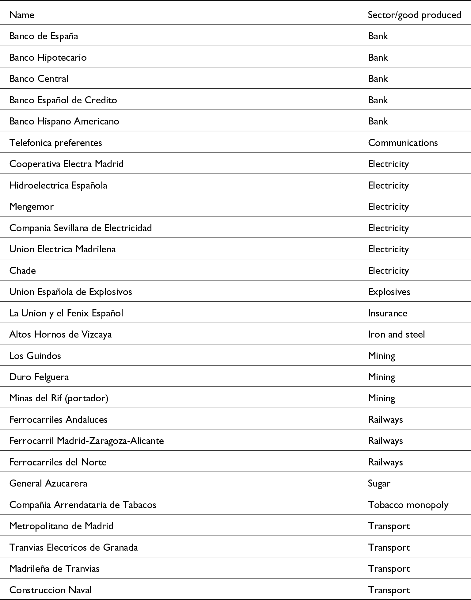
Quarterly GDP estimates for the Spanish economy during the interwar period are not yet available. Instead, I use the Economic Activity Index (EAC) developed by Albers (Reference Albers2018) to better understand the period’s dynamics. EAC does not make any ex-ante assumptions about the weights of any particular industry or indicator. The weights are determined by the strength of comovement between a given indicator and the others. This provides a broader understanding of the economy’s dynamics at the time. Figure A1a in the appendix shows that economic activity accelerated substantially from mid-1927, when banks’ holdings of public debt began to outpace their portfolios of bills of exchange (Figure 8a). There are two price indexes available. On the one hand, Prados de la Escosura (Reference Prados de la Escosura2003) provides the annual GDP deflator from 1850. On the other hand, Maluquer de Motes (Reference Maluquer de Motes2013) elaborated a consumer price index for the period 1830–2012, which includes monthly data for some groups of goods and periods. In addition, I collect a third series from the Statistical Yearbook (Anuario Estadistico) of the National Institute of Statistics (INE), which contains monthly information on prices at the individual-good level. The INE also compiled a monthly price index for consumer goods, agricultural goods, imports, and exports. Figure A1b in the appendix shows the three different price indexes: the CPI and the agricultural price index elaborated by the INE, and the WPI for the city of Barcelona elaborated by Maluquer de Motes (Reference Maluquer de Motes2013). All indexes are originally provided monthly, so I average them to obtain quarterly data. As expected, the agricultural price index is much more volatile than the other two; seasonality is slightly washed away by the other two indexes. All regressions include an index of the Madrid Stock Market as a control. I construct the index by averaging the prices of the 27 main shares quoted in Madrid, which I obtained from the Boletín Oficial de Cotizaciones of the Bolsa de Madrid. I use end-of-quarter observations for the period 1922q4–1934q4. Table A7 in the appendix contains a summary of the shares used. The resulting index is plotted in Figure A2 of the appendix, along with an alternative annual index developed by Hoyo Aparicio (Reference Hoyo Aparicio2007) as a benchmark for comparison. The index is included in the log-estimates.
4. Results and discussion
4.1. Results
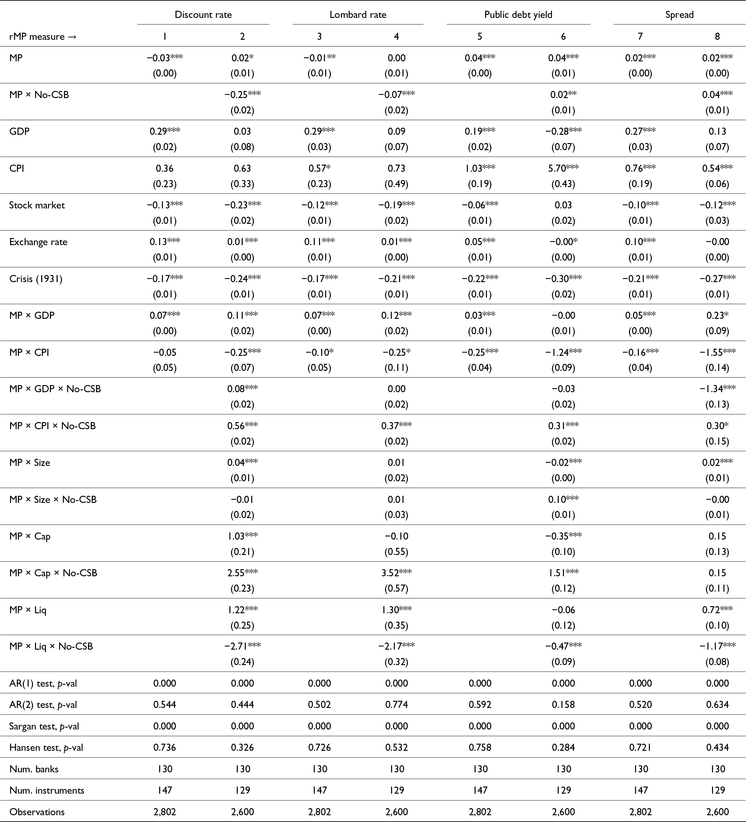
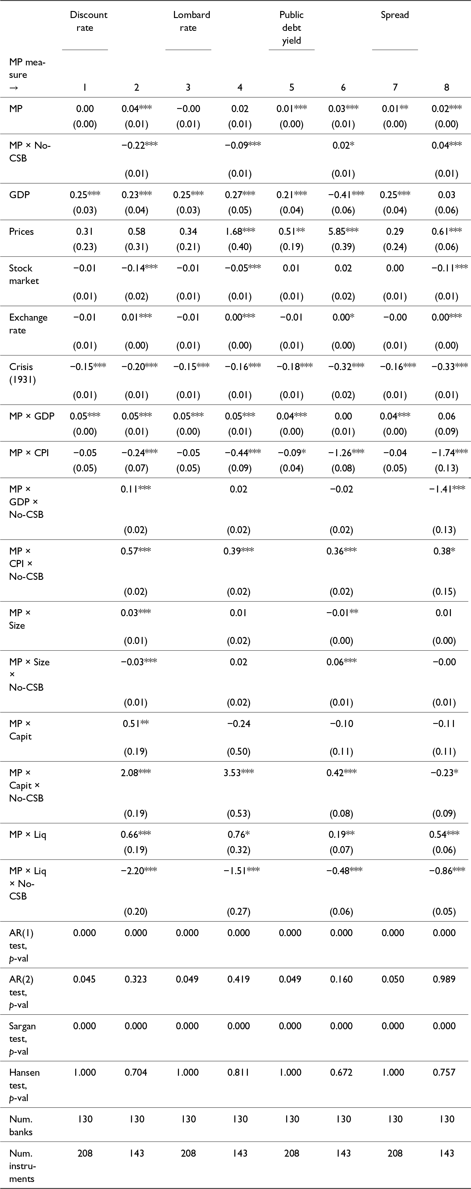
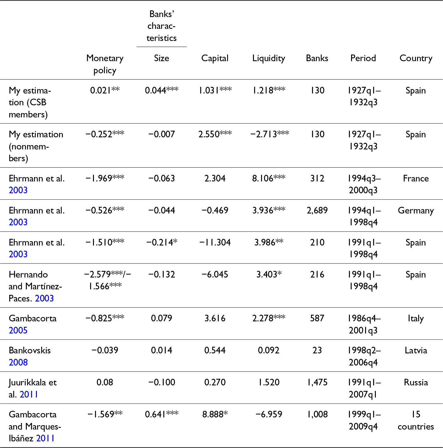
The results of estimating Equation 1 are presented in Table 4. All coefficients reported are long-run, which includes the effect of changes in the independent variable on future realizations of the dependent variable. In all specifications, the main coefficients of interest are those associated with the monetary policy indicator and its interactions with Liquidity and CSB membership (in bold). In Columns 1 and 2, the Discount rate of the BdE is used as the primary monetary policy indicator.Footnote 46 In Columns 3 and 4, the monetary policy indicator is the Lombard rate. In Columns 5 and 6, it is the yield of public debt, and in Columns 7 and 8, it is the spread between the YTM of public debt and the Lombard rate. Regression diagnostics are also reported.Footnote 47 For the sake of scaling and comparison, the main results are compared with similar estimates in the literature in Table A6 of the appendix.
Loan equation (by type of monetary policy measure), 1927q1–1932q3

Table 4 Long description
The table analyzes the impact of various monetary policy measures on financial indicators from 1927 to 1932. Key findings include significant effects of monetary policy on discount rates and public debt yields, with notable interactions during the 1931 crisis. The data reveals that GDP and CPI have varying influences across different monetary measures, with GDP generally showing positive effects and CPI showing mixed results. The stock market and exchange rates also exhibit significant responses to policy changes. The table includes statistical tests and observations, highlighting the complexity of economic interactions during this period. Interpretations should consider the historical context and the statistical significance indicated by p-values.
Note: Standard errors in parentheses, * (p < 0.1), ** (p < 0.05), and *** (p < 0.01).
Results in Columns 1 and 2 of Table 4 show that changes in the discount rate had, on average, a negative impact on bank lending (Column 1). However, the coefficient is entirely driven by nonmember banks. As a result, the negative sign of the coefficient associated with the Discount rate of the BdE disappears when the latter is interacted with the CSB membership dummy (Column 2). On average, CSB member bank lending was unaffected by changes in the discount rate. This coefficient is expected to capture the fact that CSB banks were able to avoid adjusting their loan portfolio following a change in the discount rate because they could pledge public debt at the BdE at rates below the YTM. A similar picture emerges when using the Lombard rate as the monetary policy indicator, with nonmember banks driving the negative results (Columns 3 and 4). Results in Columns 1–4 are almost identical, because when the BdE raised the Discount rate, it also raised the Lombard rate, and both were at the same level (Figure 9a). The economic magnitude of the coefficients is also relevant. For instance, in Column 2 of Table 4, the marginal effects of a one percentage point increase in the discount rate on bank lending are virtually zero for CSB member banks (0.001), but it leads to a 1.2 percentage point increase in loans for nonmembers. Similarly, in Column 4, a one percentage point increase in the Lombard rate does not change bank loans for CSB members (0.000), but it leads to a 0.8 percentage point drop in lending for nonmembers. Overall, these effects are small, but as I describe below, when balance sheet heterogeneity is introduced, the economic significance of the coefficients increases.
Because of the mechanism of indirect monetization described above, the YTM of public debt could not reflect actual monetary conditions for banks, as they could simply transform this debt into even more liquid assets, provided there was growing demand for credit. As shown above, from 1927, government debt on bank balance sheets began to grow much faster than commercial bills. This crowding-out was also evident at the BdE’s discount window, where virtually all CSB banks used public debt for Lombard lending rather than rediscounting bills of exchange. In addition, the government could issue new debt and set a specific Lombard rate for each bond type, as exemplified above. Columns 5 and 6 in Table 4 illustrate this process. When I use the yield on public debt as an indicator of monetary conditions, both groups exhibit similar behavior. The increased supply of government bonds and continued fiscal deficits led to higher yields. The results of higher yields were more than compensated by the fact that public debt could be automatically exchanged for cash at the discount window of the BdE. Columns 7 and 8 confirm that the spread between the yield of public debt and the Lombard rate was also associated with an expansion in bank loans.Footnote 48
While these results confirm contemporaries’ concerns that BdE rates were ineffective for CSB banks, they do not say much about the precise channel through which this lack of effectiveness operated. In this sense, an interesting result stands out in Table 4. Theoretical and empirical work on the transmission of monetary policy finds that, all things equal, the more liquid banks are, the less sensitive their lending is expected to be when interest rates change (Table A6). However, at odds with the consensus in the literature, all estimates in Table 4 yield a negative coefficient for the interaction between the monetary policy indicator and the liquidity ratio for nonmember banks. This would imply that, because they are more liquid than CSB members, nonmembers would respond more to changes in the BdE rate. However, this counterintuitive result arises from the way liquidity ratios are calculated. In the loan equation that I estimate in Table 4, liquidity ratios include banks’ holdings of 3-month bills of exchange, public debt, and cash as a proportion of their total assets. This is a standard definition of liquidity. However, precisely because of the argument presented in the previous sections, these three assets cannot be considered equally liquid across all banks; the BdE still retained discretion over the eligibility of bills of exchange (and would not rediscount bills held or accepted by nonmembers). However, it was forced to grant advances to CSB members when they pledged public debt. Therefore, public debt ought to have carried a substantial liquidity premium over commercial bills among banks. This implies that banks with more public debt in their portfolios should be able to increase their liabilities at cheaper rates by placing public debt with the BdE. It is precisely this ability to counter discount rate hikes by pledging public debt that is expected to eliminate the friction in reallocating liabilities that causes central bank rates to influence bank lending. Because of that, it is necessary to disaggregate the liquidity measure to identify the precise channel through which this a priori differential lending reaction based on liquidity operates.
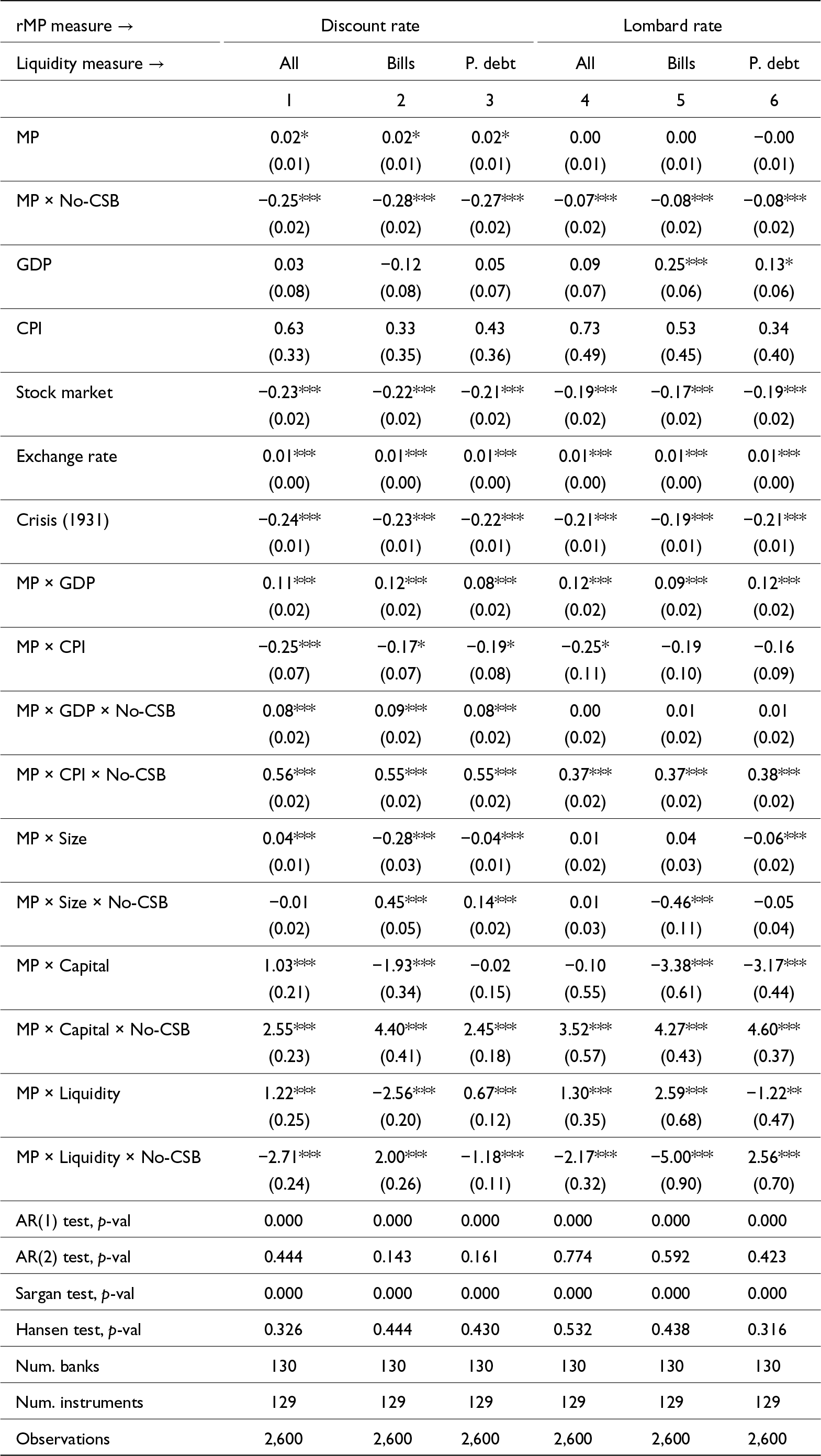
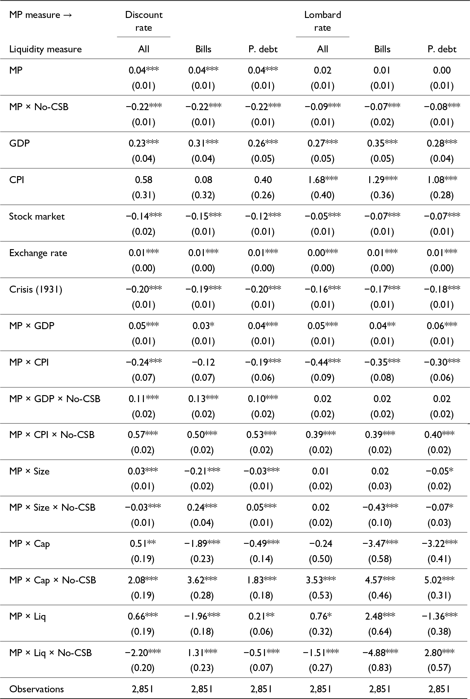
Table 5 runs six new specifications of Equation 1 with different measures of liquidity: the original measure, bills of exchange as a percentage of total portfolio, and the same for public debt. In this new specification, the sign and magnitude of the coefficients associated with the interaction between the monetary policy indicator, liquidity, and membership are intended to capture the liquidity premium that public debt carried for CSB banks. Findings provide an answer to the counterintuitive results presented in Table 4. While all other coefficients tell the same story—magnitudes being almost the same—those associated with liquidity are different. CSB members and nonmembers reacted differently to changes in BdE rates. When the BdE raised the discount rate, CSB members holding a larger share of public debt in their portfolios were not reactive to the rate change. However, those who held more bills of exchange were more likely to contract lending. This provides an explanation for the lack of transmission of BdE rate changes to bank lending, but also shows that, on average, CSB members faced a liquidity penalty for holding bills of exchange, while the contrary applied to public debt. The opposite picture comes up when I use the Lombard rate as a monetary policy indicator in Columns 4–6 in Table 5. CSB banks holding more public debt were more sensitive to changes in this rate. In terms of magnitudes, the coefficient on MP × Liquidity in Column 2 implies that a 1 percentage point increase in the discount rate led to a marginal contraction in lending for CSB banks of 2.54 percentage points. The same interaction in Column 3, with liquidity defined as the share of public debt in banks’ portfolios, implies that CSB banks continued to expand their portfolios by 0.69 percentage points despite changes in the discount rate for each additional unit of liquidity above the average. In other words, CSB banks backed their loan expansion by subscribing to public debt, and this rendered the discount rate ineffective, while for nonmembers this was not an equally viable strategy. This explains why CSB banks continued to accumulate public debt throughout the period, whereas non-CSB banks didn’t.
Loan equation (different liquidity measures), 1927q1–1932q3

Table 5 Long description
The table analyzes the impact of monetary policy measures on various liquidity measures from 1927 to 1932, focusing on discount and Lombard rates. Key findings include significant negative effects of monetary policy when no central bank support is present, particularly during the 1931 crisis. Interactions with GDP and CPI show varied impacts, with GDP generally enhancing liquidity while CPI interactions are mixed. The stock market consistently shows negative correlations with liquidity measures. Tests for autocorrelation and instrument validity indicate robust results, with significant p-values for AR(1) and Sargan tests. The data covers 130 banks and 2,600 observations, providing a comprehensive view of the period's financial dynamics.
Note: Standard errors in parentheses, * (p < 0.1), ** (p < 0.05), and *** (p < 0.01).
In sum, the results from Tables 4 and 5 confirm that rate changes implemented by the BdE during years when the peseta depreciated had no effect on bank lending to CSB members. This reflects the conflicting goals that emerged from the 1921 Banking Law, as outlined in the previous sections. While CSB banks were precisely the group of banks that were supposed to be the target of the BdE’s interest rate policy, they had a mechanism to avoid that, rooted in the political economy and the timing that dominated the negotiations of the 1921 Banking Law.
4.2. Discussion
As the government and the BdE discussed the first increase in the Discount rate in 1928 in order to curb the increase in the money supply and stem the depreciation of the peseta, contemporaries were aware that it would have little, if any, effect. As it was put at the time, for most of the year 1928, “conditions in the market were exactly the same as in 1927.”Footnote 49 According to contemporary observers, large banks appeared to have less pressure to adjust their loan portfolio than smaller banks.Footnote 50 Referring to the changes in the discount rate, in January 1930, the Finance Minister wrote a piece in El Economista, in which he argued that in Spain, “experience has shown that the variations of the discount rate have very scarce influence in the market.”Footnote 51 The limited impact on the market was a cause of concern at the time, as “there was the risk that the raise in the official rate might not be followed by the market, as it seems that there is plenty of pesetas in the money market.”Footnote 52 Hence, a final relevant question is to what extent the expansion in bank loans during the period would have been smaller enough to make a difference in the evolution of the money supply, had the system of public debt monetization set by the 1921 Banking Law not been in place.
To illustrate this, I calculate the magnitude of the difference in monetary policy transmission between CSB and non-CSB member banks. This allows for calculating a counterfactual credit expansion assuming that CSB banks reacted as non-CSB banks to changes in the BdE discount rate, holding within-group heterogeneity in the composition of the portfolios constant. To be sure, and as explained above, this is not a clean counterfactual case, because non-CSB banks self-selected into their categories, but it can illustrate the approximate importance of this mechanism for the macroeconomy. To do so, I consider the increase in the BdE discount rate from 4% to 5% between 1928 and 1930.Footnote 53 According to the estimates reported in Table 4, the coefficient on MP is 0.02 for CSB banks, and the overall coefficient is −0.223 for non-CSB banks. Applying the −0.23 coefficient to CSB banks results in their lending counterfactual lending being approximately 5% lower (0.223 × −0.25 = −0.056) in the long run. These magnitudes increase if I relax the assumptions on portfolio compositions. Assuming that CSB banks would hold public debt portfolios similar to non-CSB banks, that is, around 50% smaller—as per Table 3—then the results are larger. If I use the coefficient of the interaction MP × Liquidity × No-CSB in Column 3 of Table 5, defining MP as the discount rate and Liquidity as the share of public debt over total securities, the long-run marginal effect of MP on loan growth for non-CSB banks is estimated at −0.76 (assuming capitalization and size remain constant). If CSB banks had held similar public debt portfolios as the ones held by non-CSB banks, then the increase in the discount rate from 4% to 5% over the period would have led to an approximate 15.5% contraction in their loan portfolios. By March 1931, total bank loans in pesetas stood at 3,213 million pesetas; the counterfactual estimate implies a total stock of bank loans at 2,714 million pesetas, that is, around 500 million pesetas lower.
It is out of the scope of this paper to directly tackle the causal effect of the expansion in bank lending and the evolution of the exchange rate. However, given the correlation between the credit boom and the evolution of the exchange rate illustrated in Figure 1 and estimated in Footnote 1, it is plausible to think that the attenuation of the lending boom would have resulted in a softer exchange rate depreciation. The fall of the peseta was, in fact, the main underlying reason for which interest rates were raised during the period, as discussed above. Assuming that the stock of bank loans would have been 500 million pesetas lower if CSB banks had been responsive to interest rate changes, by March 1931, the peseta would have been at 36 pesetas per Sterling rather than 45. Admittedly, these conclusions should be taken with caution—for one, the depreciation of the peseta between 1928 and 1931 was affected by domestic political factors and international financial conditions as well. However, these back-of-the-envelope calculations illustrate how CSB membership and the content of the 1921 Banking Law insulated most Spanish banks—CSB members—from the effects of the monetary policy instruments used by monetary authorities, and this had substantial effects on the total amount of bank lending during the 1927–1931 lending boom. It further suggests that during the 1920s, fiscal policy and the system of public debt monetization through the banking system entered into conflict with the exchange-rate stabilization aimed at by policymakers.
5. Conclusion
After World War I, and in need of funding a large government debt issue, the Spanish Government established a system of “indirect monetization” of public debt through which banks were allowed to borrow from the BdE using government bonds at subsidized rates. This regime was embodied in the 1921 Banking Law, which was enacted in response to the banking crisis and the sudden need to finance a large government debt issuance. Policymakers in the Ministry of Finance emphasized panic and liquidity as the main causes of the 1920 banking crisis and shaped monetary policy and banking regulation to ensure bank liquidity and strong demand for public debt. During the second half of the 1920s, fiscal expenditure accelerated under the Primo de Rivera Dictatorship, while fiscal revenue did not keep pace, owing to the absence of effective fiscal reform. This resulted in banks’ accumulation of large public debt portfolios and revealed the contradiction between fiscal policy and exchange rate stability that fiscal authorities faced in 1921. Absent stronger fiscal revenue, fiscal policy could quickly become incompatible with attempts at a stable exchange rate—the reputational cornerstone of the Dictatorship’s economic plan—as public debt-filled banks could become nonreactive to monetary policy rate changes. When the peseta began to depreciate rapidly from 1928, all attempts to stabilize it were fruitless: with one hand, the government persuaded the BdE to raise its interest rates, while with the other, it kept running fiscal deficits. As a result of the 1921 Banking Law, monetary policy tools that were supposed to be the device to “command the credit of the nation” as per the BdE Statutes, were deemed ineffective and proved an obstacle to contain the fall of the peseta.
Acknowledgements
I am grateful to Olivier Accominotti and Stefano Ugolini for continuous support, feedback, and comments on previous versions. I am greatly indebted to Thilo N. H. Albers for taking the time to teach me how to assemble the database I use in the paper. Comments from Pablo Martin-Aceña, Elena Martínez, Harold James, M. Ángeles Pons, participants at the EHES Conference Tübingen, and from three anonymous referees helped improve the paper. All errors are mine. I acknowledge funding from the Economic and Social Research Council (Grant number: 1509253) and the LSE Radwan Travel Fund.
A. Appendix
A1. Bank balance sheet data
Data on individual bank balance sheets were collected and digitized from the Boletines del CSB, which are available at the quarterly level, for each quarter between 1922q4 and 1934q4 for the universe of Spanish banks, including foreign banks’ branches operating in Spain. After 1934, data are not comprehensive, as some banks did not report their balance sheets, and the outbreak of the Spanish Civil War brought the publication of the Boletines to a halt. Table A1 presents the names of the banks included in the sample, their size, the size of their loan portfolios, and the share of loans relative to assets. Balance sheets reported by banks include item-level data on assets and liabilities. Although I don’t use all items in this article, the list of balance sheet items available is provided below with clarification when needed:
Assets (Activo)
– Cash and banks (Caja y bancos)
* Cash at the bank and at Banco de España (Caja y Banco de España)
* Cash in foreign exchange (Moneda y billete extranjero)
* Interbank assets (Bancos y banqueros)
– Securities (Cartera)
* 90-day bills of exchange (Efectos de comercio 90 días)
* Over 90-day bills of exchange (Efectos de comercio, más de 90 días)
* Public debt (Fondos públicos)
* Other securities (Otros valores)
– Loans (Créditos)
* Loans on collateral (Deudores con garantía prendaria)
* Call loans (Deudores a la vista)
* Long-term loans (Deudores a plazo)
* Foreign exchange loans (Deudores en moneda extranjera)
– Others (Otros)
* Real Estate (Inmuebles)
* Furniture and installations (Mobiliario e instalaciones)
* Shareholders (Accionistas)
* Own shares (Acciones en cartera)
* Acceptances (Deudores por aceptaciones)
* Other accounts (Otras cuentas)
Liabilities (Pasivo)
– Capital (Capital)
– Reserves (Reservas)
* Reserves (Reservas)
* Provision for losses on securities (Fondo de fluctuacion de valores)
– Depositors (Acreedores)
* Interbank deposits (Bancos y banqueros)
* Call deposits (A la vista)
* Up to 1 month deposits (Hasta un mes)
* Longer term (A mayores plazos)
* In foreign exchange (En moneda extranjera)
– Bills payable (Efectos y demás obligaciones a pagar)
– Acceptances (Aceptaciones)
– Other accounts (Otras cuentas)
Macroeconomic variables, 1922–1935.

Figure A1 Long description
The image contains two graphs. (a) Economic Activity graph shows data from December 1923 to August 1935 with three lines: 'Produccion Industrial - INE', 'Albers and Uebele (2015)' and 'Interpolated (Prados de la Escosura, 2003)'. The y-axis ranges from 90 to 120. (b) Prices graph displays data from December 1922 to August 1934 with three lines: 'CPI (INE)', 'Agric CPI (INE)' and 'WPI Barcelona (Maluquer de Motes, 2013)'. The y-axis ranges from 150 to 220. Both graphs illustrate trends and fluctuations over time.
Banks’ names, membership, and size of loan portfolio (thousand pesetas, in 1928q3)

Table A1 Long description
The table provides data on banks' names, codes, loan amounts, total assets, and the ratio of loans to assets in thousand pesetas for the third quarter of 1928. Banco Pastor leads with the largest loan portfolio of 221,702 thousand pesetas, whereas Banco de Tolosa has the lowest loans-to-assets ratio at 4%. Banco de Santander has the highest loans-to-assets ratio at 66%, indicating a high proportion of loans relative to its assets. Notably, Banco Español de Credito and Banco Popular Previsores Porvenir also have significant loan portfolios, each exceeding 200,000 thousand pesetas. The data suggests a wide variation in the financial strategies of these banks, with some focusing heavily on loans while others maintain a more balanced asset distribution.
A2. Selected macroeconomic variables
Madrid stock market index, 1922–1934 (1926q1 = 100).

Figure A2 Long description
A line graph showing the Madrid stock market index from 1922 to 1934. The x-axis represents time from December 1922 to December 1934 and the y-axis represents the index value ranging from 80 to 170. The graph includes two data series: the end-of-quarter index represented by a line and the Hoyo Aparicio data represented by dots. The index shows a significant rise starting around 1927, peaking between 1929 and 1930, followed by a decline. The Hoyo Aparicio data points are scattered along the timeline, providing additional reference points for comparison.
Banks’ names, membership, and size of loan portfolio (thousand pesetas, in 1928q3)

Table A2 Long description
The table compares banks' names, codes, loan amounts, total assets, and the ratio of loans to assets in thousands of pesetas for the third quarter of 1928. Lazard Brothers stands out with the highest loans-to-assets ratio at 58%, suggesting a strong focus on lending relative to its asset base. In contrast, Banco de Valls and Francisco Lopez have no loans, indicating either a conservative approach or a different business model. Banco Urquijo de Madrid has the largest loan portfolio at 148,881 thousand pesetas, highlighting its significant lending capacity. The loans-to-assets ratio varies widely among banks, from 0% to 58%, reflecting diverse financial strategies and risk profiles. This data provides insight into the banking landscape of the time, with some banks prioritizing asset accumulation over lending.
A3. Alternative time spans
Banks’ names, membership, and size of loan portfolio (thousand pesetas, in 1928q3)

Table A3 Long description
The table provides data on various banks, focusing on their loan portfolios and assets in thousand pesetas for the third quarter of 1928. Union Iberica Mobiliaria e Inmobiliaria stands out with the highest loans-to-assets ratio of 70%, suggesting a significant portion of its assets are tied up in loans. In contrast, banks like Bonifacio Cano y Cano and M. Bruguera Sabater have a loans-to-assets ratio of 0%, indicating they have no loans against their assets. Banco de Burriana also shows a high ratio of 49%, while Banco de Ferrerias has the lowest at 1%. The data highlights a wide range of financial strategies among these banks, with some focusing heavily on loans and others maintaining more liquid asset bases. This variation could reflect differing business models or market conditions faced by these institutions.
A4. Comparison with other estimates in the literature
Loan equation (by type of monetary policy measure), 1926q1–1933q4

Table A4 Long description
The table examines the effects of different monetary policy measures, such as discount and Lombard rates, on economic indicators between 1926 and 1933. Key findings include significant positive impacts of GDP on all measures, with the strongest effect on the Lombard rate. The 1931 crisis consistently shows a negative impact across all measures. The interaction of monetary policy with GDP and consumer price index reveals varying effects, with notable significance in the absence of central bank support. The table also includes statistical tests for model validity, indicating robust results. Standard errors and significance levels are provided, suggesting careful consideration of statistical reliability.
Note: Standard errors in parentheses, * (p < 0.1), ** (p < 0.05), and *** (p < 0.01).
A5. Stock market index composition
Loan equation (by type of monetary policy and liquidity measure), 1926q1–1933q4

Table A5 Long description
The table analyzes the impact of monetary policy measures, specifically the discount and Lombard rates, on loan equations from 1926 to 1933. Key findings include the discount rate having a more pronounced effect on loans compared to the Lombard rate, particularly when interacting with GDP and CPI. The interaction of monetary policy with GDP shows a positive effect, while its interaction with CPI generally results in a negative effect. The presence of a crisis in 1931 consistently shows a negative impact across all measures. Observations remain constant at 2851, and standard errors are provided for each data point, indicating statistical significance at various levels.
Note: Standard errors in parentheses, * (p < 0.1), ** (p < 0.05), and *** (p < 0.01).
Comparison of the estimation results with the literature on monetary policy transmission

Table A6 Long description
The table compares estimation results of monetary policy transmission across various studies, focusing on bank characteristics like size, capital, and liquidity. Key findings include significant positive effects on liquidity for CSB members in Spain from 1927 to 1932, while non-members show negative effects. Ehrmann's study in France from 1994 to 2000 shows a strong positive liquidity effect, contrasting with negative monetary policy effects. Gambacorta's research in Italy from 1986 to 2001 indicates a positive liquidity impact. The data reveals diverse impacts of monetary policy across countries and periods, with Spain showing both positive and negative effects depending on the study and bank membership status. These variations suggest that monetary policy transmission is influenced by specific bank characteristics and economic contexts.
Shares included in the index and the type of firm

Table A7 Long description
The table categorizes firms by their sector or the goods they produce, highlighting a diverse range of industries. The banking sector is the most represented, with five entries including Banco de España and Banco Hipotecario. The electricity sector follows closely, featuring companies like Cooperativa Electra Madrid and Hidroelectrica Española. Other sectors include communications, insurance, iron and steel, mining, railways, sugar, tobacco monopoly, and transport. Notably, the transport sector includes both railways and tram services, indicating a focus on different modes of transportation. This distribution suggests a historical emphasis on financial services and utilities within the index.