1 INTRODUCTION
1.1 Motivation
Recent decades have witnessed surged interests in the econometrics and causal inference literature on the construction of nearly rate-optimal estimators for parameters/estimands/(statistical) functionals, such as the average treatment effect (ATE). One particular fruitful econometric paradigm is through the lens of semiparametric theory (Schick, Reference Schick1986; Newey, Reference Newey1990), which delivers, among other things, the celebrated doubly-robust augmented inverse probability weighting (AIPW) estimator of the ATE (Robins, Rotnitzky, and Zhao, Reference Robins, Rotnitzky and Zhao1994; Hahn, Reference Hahn1998; Chernozhukov et al., Reference Chernozhukov, Chetverikov, Demirer, Duflo, Hansen, Newey and Robins2018), based on the (first-order) influence function of the target parameter. The asymptotic variance of such estimators is known to achieve the semiparametric efficiency bound, provided that sufficient complexity-reducing assumptions are imposed on the nuisance parameters (the outcome regression and the propensity score in the case of ATE).
1.1.1 Sub-Optimality of First-Order Estimators
Despite the popularity of estimators based on influence functions (henceforth, first-order estimators), growing evidence suggests that they can be sub-optimal in certain settings. Specifically, even when the parameter of interest is estimable at the parametric
$n^{-1/2}$
 rate, first-order estimators may fail to achieve
$n^{-1/2}$
 -consistency, letting alone attain the semiparametric efficiency bound. This sub-optimality can arise in a variety of contexts, including, for example, when the nuisance parameters are assumed to belong to Hölder-type smoothness classes (Liu et al., Reference Liu, Mukherjee, Newey and Robins2017; Robins et al., Reference Robins, Li, Liu, Mukherjee, Tchetgen Tchetgen and van der Vaart2023), structure-agnostic classes for certain types of parameters (Robins and Ritov, Reference Robins and Ritov1997; Liu, Mukherjee, and Robins, Reference Liu, Mukherjee and Robins2024; Jin and Syrgkanis, Reference Jin and Syrgkanis2025; Balakrishnan, Kennedy, and Wasserman, Reference Balakrishnan, Kennedy and Wasserman2026; Liu, Mukherjee, and Robins, Reference Liu, Rajarshi Mukherjee and Robins2026), or hybrid smoothness–structure-agnostic classes (Bonvini et al., Reference Bonvini, Kennedy, Dukes and Balakrishnan2024); or when the nuisance parameters are in the many-covariate or small-bandwidth settings, where a direct plug-in estimator based on first-order influence functions possibly may lead to a “leave-in” bias (Cattaneo and Jansson, Reference Cattaneo and Jansson2018; Cattaneo, Jansson, and Ma, Reference Cattaneo, Jansson and Ma2019).
Using ATE and classical nonparametric nuisance models as an illustration, when both the outcome regression and the propensity score belong to Hölder smoothness classes with smoothness index s and variable dimension d, standardFootnote
1
first-order estimators of ATE are
$n^{-1/2}$
 -consistent when
$\frac {2 s / d}{1 + 2 s / d}> 0.5$
 , that is,
$s / d> 0.5$
 . However, it is well known that
$s / d> 0.25$
 is both sufficient and necessary (hence minimal) for ATE to be
$n^{-1/2}$
 -estimable (Robins et al., Reference Robins, Tchetgen Tchetgen, Li and van der Vaart2009, Reference Robins, Li, Liu, Mukherjee, Tchetgen Tchetgen and van der Vaart2023). Indeed, estimators based on higher-order influence functions (HOIFs) (Robins et al., Reference Robins, Li, Tchetgen Tchetgen and van der Vaart2008, Reference Robins, Li, Tchetgen Tchetgen and van der Vaart2016; Liu et al., Reference Liu, Mukherjee, Newey and Robins2017), a generalization of the classical first-order influence functions, have been shown to be
$n^{-1/2}$
 -consistent for ATE when
$s / d> 0.25$
 (Liu et al., Reference Liu, Mukherjee, Newey and Robins2017; Robins et al., Reference Robins, Li, Liu, Mukherjee, Tchetgen Tchetgen and van der Vaart2023). In the remainder of this article, we refer to these estimators as the “higher-order estimators” (HOEs) for convenience. More importantly, to the best of our knowledge, no other simpler estimators are
$n^{-1/2}$
 -consistent under this minimal Hölder smoothness condition, despite years of research efforts. These results also prompt recent advances in applying the HOIF framework to statistical problems similar to but more complex than ATE, such as conditional ATEs (Kennedy et al., Reference Kennedy, Balakrishnan, Robins and Wasserman2024) and average dose–response functions (ADRFs; Bonvini and Kennedy, Reference Bonvini and Kennedy2022; Colangelo and Lee, Reference Colangelo and Lee2026). Our approach is also connected to the literature addressing “leave-in bias” in the many-covariate and small-bandwidth settings (Cattaneo and Jansson, Reference Cattaneo and Jansson2018; Cattaneo et al., Reference Cattaneo, Jansson and Ma2019); see Section 1.2, Remark 8, and Section S5 of the Supplementary Material for an extended discussion. The present article extends this line of work to a broader class of parameters central to modern econometric analysis, which will be made precise next.
1.1.2 Challenges Due to Implicitly-Defined Parameters
The existing HOIF framework primarily concerns parameters that are explicitly defined, including but not limited to ATE and parameters used in conditional independence tests (Shah and Peters, Reference Shah and Peters2020) as prominent examples. However, many causal parameters of interest in modern economics applications lack closed-form expressions and are instead defined as solutions to moment conditions or optimization problems. The quantile treatment effect (QTE) provides a canonical example. In policy evaluation, when outcomes are heterogeneous or heavy-tailed, QTE offers a more informative summary of treatment effects than the mean (Manski, Reference Manski2004; Chernozhukov and Hansen, Reference Chernozhukov and Hansen2005; Firpo, Reference Firpo2007; Powell, Reference Powell2020). Yet, QTE can only be characterized as the solution to a variational problem (M-estimation) or to a moment equation (Z-estimation) (see Example 2 later). Another prominent example in the recent econometrics literature is the
$\alpha $
 -expected shortfall (ES; Fan, Qi, and Xu, Reference Fan, Qi and Xu2025), which measures the average outcome in the worst
$\alpha $
 fraction of the distribution. This quantity is of particular interest in risk management and policy evaluation under tail risk, where policymakers are concerned with extreme rather than average outcomes. Borrowing a terminology from Robins et al. (Reference Robins, Li, Tchetgen Tchetgen and van der Vaart2016), such parameters are implicitly defined. These implicitly defined parameters can pose significant challenges to estimation and inference.
Another important challenge arises from the non-separability between the nuisance parameter and the parameter of interest (Su, Ura, and Zhang, Reference Su, Ura and Zhang2019; Chernozhukov et al., Reference Chernozhukov, Deaner, Gao, Hausman and Newey2025). Using QTE with binary treatment as an example, as shown in Example 2 and Remark 2 later, one of the nuisance parameters, the generalized outcome regression model, depends on the true but unknown QTE parameter. To address this problem, Kallus et al. (Reference Kallus, Mao and Uehara2024) develop the localized debiased machine learning (LDML) estimator, which first produces an initial estimator of the QTE using only the propensity score independent of the QTE itself. With this initial estimator, LDML proceeds to estimate the generalized outcome regression model and then constructs a rate doubly-robust estimator based on the influence function of the QTE. However, as shown in Kallus et al. (Reference Kallus, Mao and Uehara2024) and for the sake of completeness in Section 2.2, for the LDML estimator to be
$n^{-1/2}$
 -consistent, it demands certain strong assumptions on the rate of convergence of the initial QTE estimator, hence also on the regularity of the propensity score (see Proposition 2). Ai et al. (Reference Ai, Linton, Motegi and Zhang2021) bypass the two-step procedure and estimate the QTE by using only the propensity score. But unlike the LDML estimator, the QTE estimator of Ai et al. (Reference Ai, Linton, Motegi and Zhang2021) fails to be rate double-robust. It is then natural to raise the following question:
Can estimators of QTE or other more general implicitly-defined causal parameters be constructed that improve upon existing ones based on influence functions, in terms of convergence rates and the required assumptions on the initial estimators?
We provide a positive answer to the above inquiry by going beyond the classical first-order semiparametric theory, in a sense formalized later in the article. For implicitly defined parameters, however, the literature beyond first-order estimators is rather scarce, with the only exception being Section 6 of Robins et al. (Reference Robins, Li, Tchetgen Tchetgen and van der Vaart2016), which touches on the issue without providing a treatment with further technical details. Also, the regression slope in a partially linear model was considered in Robins et al. (Reference Robins, Li, Tchetgen Tchetgen and van der Vaart2016) as a leading example, which has an explicit form.Footnote 2 Our article partially fills this gap. To strike a balance between the generality and practical utility of our results, we opt for considering a broad class of parameters defined via generic moment equations with possibly non-smooth, non-separable generalized residual functions (see (1)). This formulation accommodates discrete, continuous, and more complicated treatment types in a unified way, and it aligns with a growing econometrics literature that represents causal targets through generic moments. For example, Ao, Calonico, and Lee (Reference Ao, Calonico and Lee2021) use a generic moment function applied to counterfactual distributions under multivalued treatments. Within this unified formulation, we cover a wide range of parameters encountered in applied causal inference, including ATE, QTE, and more generally the general treatment models (GTMs) recently coined in the econometrics literature (Ai et al., Reference Ai, Linton, Motegi and Zhang2021; Chen and Xie, Reference Chen and Xie2025). Extending the HOIF framework to parameters of GTMs is thus instrumental toward building a broadly applicable point and interval estimation scheme for parameters encountered in econometrics.
1.1.3 Summary of Main Results and Contributions
Compared to the HOIF theory for explicitly defined parameters, the following challenges remain to be addressed, which constitute the main contributions of our article.
-
(1) We derive HOIFs for causal parameters implicitly defined through GTMs, facilitating the construction of improved higher-order estimating equations, compared to state-of-the-art estimators based on the first-order theory, such as the LDML estimator. While we mainly analyze estimators solving second-order estimating equations, we refer to them as HOEs to avoid introducing additional terminology, and we also present the full m-th-order construction in Section S3 of the Supplementary Material. Among the parameters of GTMs, the QTE with binary treatment is one of the most commonly encountered examples in practice. We obtain an $n^{-1/2}$
 -consistent estimator for QTE under the weakest Hölder smoothness assumptions on the nuisance parameters to date, almost matching the minimal smoothness assumptions for ATE to be
$n^{-1/2}$
-estimable.
-
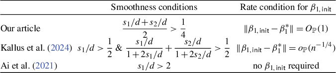
(2) State-of-the-art first-order estimators require an initial estimator of the target parameter to estimate the nuisance parameters. This extra step incurs an additional rate condition on the initial estimator and, consequently, on certain nuisance parameter(s). As we will see in Section 3.4, for the QTE with binary treatment, our proposed HOEs can drastically relax this rate condition, highlighting another advantage of HOEs (see Table 1 in Section 3.4).
-
(3) The original formulation of GTMs by Ai et al. (Reference Ai, Linton, Motegi and Zhang2021) assumes a parametric specification for the target parameters. When the treatment takes finitely many discrete values, finite-dimensional GTMs are effectively nonparametric. However, in many modern applications, treatment variables are often continuous. It may then be necessary to consider infinite-dimensional GTMs to avoid model misspecification bias; or otherwise, the finite-dimensional GTMs can at best be interpreted as a projection of the true causal or structural parameters onto a parametric model. To our knowledge, Colangelo and Lee (Reference Colangelo and Lee2026) and Bonvini and Kennedy (Reference Bonvini and Kennedy2022) are among the first to consider estimating the ADRF (see Example 7 later) using HOEs when the treatment is continuous. To incorporate such scenarios, we extend our HOEs to nonparametric GTMs, thereby generalizing the results of Colangelo and Lee (Reference Colangelo and Lee2026) and Bonvini and Kennedy (Reference Bonvini and Kennedy2022) to include, for example, the quantile dose–response function (QDRF) (see Example 8 later).


Before proceeding, we illustrate the value of incorporating HOIF theory for GTM parameters through a simulation study; full details are provided in Sections 3.1 and 5.1. For clarity of exposition, we present the discussion at a high level and defer some technical rigor to later sections. Figure 1 reports the simulation results. The parameter of interest
$\beta ^{*}$
 is the QTE at the
$25\%$
 quantile, with binary treatment and a one-dimensional covariate that suffices to control for confounding. The histograms display the simulated distribution of the centered estimator,
$\widehat {\beta }-\beta ^{*}$
 . In the left panel of Figure 1, we adopt the aforementioned state-of-the-art LDML estimator (Kallus et al., Reference Kallus, Mao and Uehara2024), with nuisance parameters (see Example 2 later) estimated by neural networks (Chen et al., Reference Chen, Liu, Ma and Zhang2024a). We design the simulation such that the nuisance parameters have low smoothness in Hölder sense (with smoothness close to
$s = 0.4$
 ). As a result, even LDML with neural networks fails to deliver an estimator that is close to being unbiased, which is not too surprising given the empirical evidence on the difficulty of fitting functions of low regularity by neural networks in practice (Xu, Liu, and Liu, Reference Xu, Liu and Liu2022). In contrast, the right panel of Figure 1 shows that, after centering by the true QTE, our HOIF-based estimator is well centered around zero, though with slightly higher variance than the LDML estimator. This empirical result demonstrates that the HOIF framework can be a useful tool even when modern neural networks are employed for nonparametric first-step estimation, complementing state-of-the-art methods based on classical semiparametric theory.
Comparison between the first-order (LDML) estimator and the higher-order estimator (HOE) of QTE. The histograms over 1,000 Monte Carlo simulations are displayed, and the red curves are the corresponding normal probability density function with the same mean and variance as the Monte Carlo mean and variance.
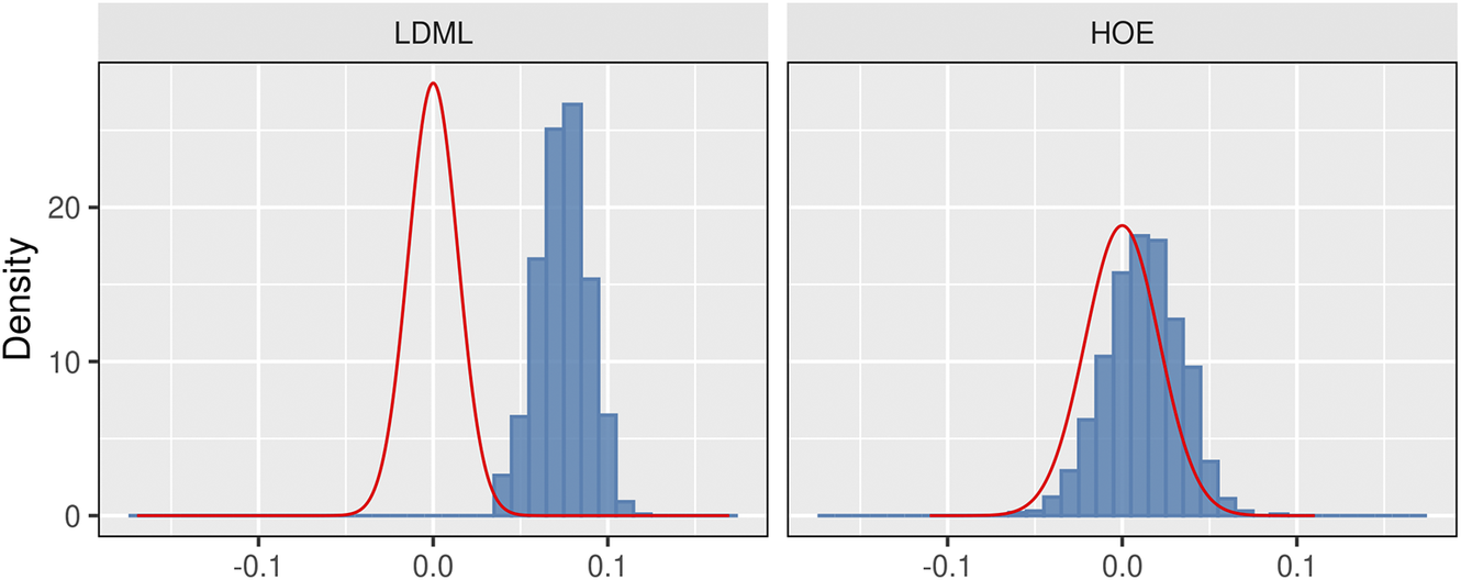
Figure 1 Long description
Two panels arranged horizontally share a common Y-axis labeled Density with increments of 0, 10, and 20. The X-axis for both ranges from minus 0.1 to 0.1.
Left Panel (L D M L): The blue histogram is concentrated on the right side of the graph, with its peak density reaching nearly 30 between 0.05 and 0.1. A red normal probability density curve is centered at 0.0, showing a significant spatial gap between the theoretical normal distribution and the actual Monte Carlo simulation data.
Right Panel (H O E): The blue histogram is centered around 0.0. The red normal probability density curve is overlaid directly on top of the histogram. The peak of the red curve and the highest blue bars both align at the 0.0 mark on the X-axis, indicating a high degree of fit between the estimator and the normal distribution.
1.2 A Survey of Related Works
Our work is related to several strands of literature in econometrics and statistics. We now give a brief (and very likely incomplete) survey.
-
(1) Two-Step Procedures: The problem studied in this article is related to classical and modern semiparametric two-step estimation in econometrics, where some first-stage nuisance components may be indexed by the target parameter. Classical semiparametric theory typically imposes conditions under which the first-stage bias is asymptotically negligible, so that the limiting distribution of the target estimator is not affected (see, among others, Newey, Reference Newey1990; Newey and McFadden, Reference Newey and McFadden1994; Chen, Linton, and Van Keilegom, Reference Chen, Linton and Van Keilegom2003, and the references therein).
More recent work develops estimation and inference procedures that remain valid when first-stage bias is non-negligible. For example, Cattaneo and Jansson (Reference Cattaneo and Jansson2018) and Cattaneo et al. (Reference Cattaneo, Jansson and Ma2019) study two-step estimators where the first-stage bias can enter the asymptotic distribution of the target parameter, using kernel-based and linear-regression-based nuisance estimators, respectively. Specifically, Cattaneo et al. (Reference Cattaneo, Jansson and Ma2019) consider a setting with many covariates, where the first-stage nuisance estimator is obtained by linear regression. They show that a non-negligible leave-in bias arises when the same sample is used for both steps, and propose jackknife-type methods to consistently estimate and remove this bias, yielding a bias-corrected estimator. Cattaneo and Jansson (Reference Cattaneo and Jansson2018) develop a small-bandwidth asymptotic framework for kernel-based first-step estimators, where the smoothing bias is not assumed negligible. They show that the standard nonparametric bootstrap automatically corrects for this bias, so that percentile confidence intervals achieve correct coverage. When the asymptotic bias cannot be consistently estimated, Cavaliere et al. (Reference Cavaliere, Gonçalves, Nielsen and Zanelli2024) propose a distributional adjustment to restore bootstrap validity. Their method first obtains a bootstrap p-value, which is not asymptotically uniform due to the bias. They show that this p-value converges to a non-uniform limit that does not depend on the bias. By applying a probability integral transformation estimated via a second bootstrap, they obtain a corrected p-value that is asymptotically uniform, thus restoring valid inference without directly estimating the bias. Cattaneo et al. (Reference Cattaneo, Farrell, Jansson and Masini2025) develop higher-order distributional approximations for kernel-based estimators of the density-weighted average derivative. By employing Edgeworth expansions, they refine the large-sample approximation of the estimator’s distribution, which leads to improved finite-sample inference, particularly enhancing the coverage accuracy of confidence intervals. Another broad class of approaches focuses on estimators with a small bias property (SBP; Newey, Hsieh, and Robins, Reference Newey, Hsieh and Robins2004), meaning that the bias of the target estimator vanishes faster than the bias of the first-stage nuisance estimators. Newey et al. (Reference Newey, Hsieh and Robins2004) show that a class of semiparametric estimators based on twicing kernels satisfy this property. Tackling a similar problem and motivated by the HOIF theory, Chen, Liu, and Mukherjee (Reference Chen, Liu and Mukherjee2024b) proposed moment-based $\sqrt {n}$
-consistent estimators of a class of causal parameters even when the nuisance parameters, assumed to be generalized linear models, are not consistently estimable. -
(2) Influence Functions and Semiparametric Inference: Our work builds on and extends semiparametric and nonparametric inference based on influence functions, which play a central role in semiparametric efficiency theory. Influence-function-based estimation is a classical topic in semiparametric theory and has been studied for decades. For example, Schick (Reference Schick1986) develops a general method for constructing asymptotically efficient estimators in semiparametric models. Newey (Reference Newey1990) provides an introduction to semiparametric efficiency bounds, discussing their nature, calculation, and application in constructing semiparametric estimators and deriving their limiting distributions. For a more detailed and comprehensive treatment of influence functions for general semiparametric models and statistical inference, see Bickel et al. (Reference Bickel, Klaassen, Ritov and Wellner1998). As mentioned, our results can be viewed as a further development of the higher-order generalization of the classical influence-function-based approaches (Robins et al., Reference Robins, Li, Tchetgen Tchetgen and van der Vaart2008).
For binary treatment, Robins et al. (Reference Robins, Rotnitzky and Zhao1994) and Hahn (Reference Hahn1998) derived the efficient influence functions for ATE and ATE on the treated (ATT). Cattaneo (Reference Cattaneo2010) considered a general treatment effect model with possibly over-identified and non-smooth moment conditions under multi-valued treatments, covering a broad class of treatment effect parameters, including ATE and QTE, and established the corresponding efficiency bounds. Building on these efficiency results, the relevant literature focuses on developing practical estimators for treatment effects (see, e.g., Hirano, Imbens, and Ridder, Reference Hirano, Imbens and Ridder2003 and the references therein). Recent work also leverages influence functions to obtain valid inference with high-dimensional or machine-learned nuisance components (Chernozhukov et al., Reference Chernozhukov, Chetverikov, Demirer, Duflo, Hansen, Newey and Robins2018). Colangelo and Lee (Reference Colangelo and Lee2026) further extend DML-type ideas to kernel-based inference on the ADRF under continuous treatments. Rotnitzky et al. (Reference Rotnitzky, Smucler and Robins2021) and Chernozhukov et al. (Reference Chernozhukov, Escanciano, Ichimura, Newey and Robins2022) characterized a large class of explicitly-defined parameters, including ATE and ATT, for which DML-type estimators can be constructed based on their influence functions. Newey and Robins (Reference Newey and Robins2018) developed refined DML-type estimators that achieve faster convergence rates under smoothness classes with different nuisance parameters estimated from different independent subsamples.
Papers mentioned above mainly concern explicitly-defined parameters, including ATE and ATT. In terms of implicitly-defined parameters, Firpo (Reference Firpo2007) studies efficient influence functions for QTE with binary treatment. Ao et al. (Reference Ao, Calonico and Lee2021) develop a unified moment-based framework for multi-valued treatments, covering means, quantiles, and distribution functions, and propose an efficient influence function-based estimator for multivalued treatment effects for the treated. Their approach also enables decomposition analysis, separating wage structure effects from composition effects. Applying their method to evaluate the Workforce Investment Act (WIA) program, they find that heterogeneity in participation levels is an important dimension for evaluating social programs, demonstrating the practical relevance of their methods for policy evaluation. Complementarily, Ai et al. (Reference Ai, Linton, Motegi and Zhang2021) provide a unified framework for continuous treatments and derive efficient influence functions for GTMs. As mentioned, more recently, Kallus et al. (Reference Kallus, Mao and Uehara2024) propose the LDML estimator for the QTE, along the line of DML estimators.

1.3 Notation
Before proceeding, we collect some frequently used notation. Let
$L_{2, 0}$
 denote the space of mean zero
$L_{2}$
 functions with respect to a dominating measure
$\nu $
 . Without loss of generality, we take
$\nu $
 to be the Lebesgue measure throughout the article. We write
$a_n \lesssim b_n$
 (resp.
$a_n \gtrsim b_n$
 ) if
$a_n \leq C b_n$
 (resp.
$a_{n} \geq C b_{n}$
 ) for some universal constant
$C> 0$
 independent of n;
$a_n \asymp b_n$
 if
$a_n \lesssim b_n$
 and
$b_n \gtrsim a_n$
 ; and
$a_n \gg b_n$
 (resp.
$a_n \ll b_n$
 ) if
$b_n/a_n \to 0$
 (resp.
$b_n/a_n \to \infty $
 ). For
$a,b \in {\mathbb {R}}$
 , let
$a \vee b = \max \{a,b\}$
 and
$a \wedge b = \min \{a, b\}$
 . For a vector
$\bar {a} \in {\mathbb {R}}^{q}$
 , let
$\| \bar {a} \| := (\bar {a}^{\top }\bar {a})^{1/2}$
 denote its Euclidean norm and
$\bar {a}^{\otimes 2} = \bar {a}\,\bar {a}^{\top } $
 denote the tensor (Kronecker) product. For a matrix
$A\in {\mathbb {R}}^{p\times q}$
 , we write its operator norm as
$ \Vert A\Vert _{\mathrm {op}} := \inf \{c>0:\,\Vert Av\Vert \le c\Vert v\Vert \ \text {for every}\ v\in {\mathbb {R}}^{q}\} $
 . Given any function
$f: {\mathcal {O}} \to {\mathbb {R}}^{m}$
 with fixed integer
$m \geq 1$
 , we denote its
$L_{\infty }$
 -norm as
$\|f (\cdot )\|_{\infty } := \sup _{o \in {\mathcal {O}}} \|f (o)\|$
 .
The HOEs introduced later involve
$L_{2} (\mathbb {P})$
 projections onto the span of a size-k dictionary
$\bar {\phi }_{k} := (\phi _{1}, \ldots , \phi _{k})$
 , where each
$\phi _{j}: {\mathcal {O}} \rightarrow {\mathbb {R}}$
 . For any
$f: {\mathcal {O}} \rightarrow {\mathbb {R}}$
 , this projection is denoted by
$\Pi (f \mid \bar {\phi }_{k}) (\cdot ) := {\mathbb {E}} \{f (O) \bar {\phi }_{k} (O)\}^{\top } \Sigma _k^{-1} \bar {\phi }_{k} (\cdot )$
 , where
$\Sigma _{k} := {\mathbb {E}} \{\bar {\phi }_{k} (O)^{\otimes 2}\}$
 is the population Gram matrix. The orthocomplement of this projection is
$\Pi ^{\perp } (f \mid \bar {\phi }_{k}) (\cdot ) := f (\cdot ) - \Pi (f \mid \bar {\phi }_{k}) (\cdot )$
 .
For any measurable function
$h: {\mathcal {O}}^{m} \rightarrow {\mathbb {R}}$
 , let
${\mathbb {U}}_{n, m}$
 be the m-th-order U-statistic operator:

${\mathbb {U}}_{n, 1} \equiv {\mathbb {P}}_{n}$
 is understood to be the empirical mean.
We next review some basic concepts from empirical processes theory (see van der Vaart and Wellner, Reference van der Vaart and Wellner2023, for further details). For a probability measure Q and a constant
$p> 1$
 , let
$\| \cdot \|_{Q,p}$
 denote the
$L_{p} (Q)$
 -seminorm, that is,
$\|f\|_{Q, p} := \{\int |f (x)|^{p} {\mathrm d} Q (x)\}^{1/p}$
 for finite p while
$\|f\|_{Q,\infty }$
 denotes the essential supremum of
$|f|$
 with respect to Q. Let
${\mathcal {F}}$
 be a class of symmetric measurable functions
$f : {\mathcal {O}}^{m} \rightarrow {\mathbb {R}}$
 with envelope
$\mathrm {F}$
 , that is,
$\sup _{f\in {\mathcal {F}}} |f| \leq \mathrm {F} $
 . If
$\| \mathrm {F} \|_{Q,p}> 0$
 , we write
$\mathsf {N} ( {\mathcal {F}},\|\cdot \|_{Q,p} , \epsilon \|\mathrm {F}\|_{Q,p})$
 for the minimal number of
$\|\cdot \|_{Q,p}$
 -balls of radius
$\epsilon \|\mathrm {F}\|_{Q,p}$
 needed to cover
${\mathcal {F}}$
 . We finally recall the following definition.
Definition 1 (VC-Type Class)
A function class
${\mathcal {F}}$
 with envelope
$\mathrm {F}$
 is said to be of VC type with characteristic
$(A, v)$
 if
$\sup _{Q} \mathsf {N} \left ( {\mathcal {F}}, \| \cdot \|_{Q, 2}, \epsilon \| \mathrm {F} \|_{Q, 2} \right ) \leq (A / \epsilon )^{v}$
 for all
$\epsilon \in (0, 1]$
 , where
$\sup _{Q}$
 denotes the supremum over all discrete finite probability measures.
For vector-valued functions
${\mathcal {F}} := \{f: \mathcal O^{m} \to {\mathbb {R}}^{q}\}$
 (with fixed q), these definitions are interpreted with
$|\cdot |$
 replaced by the Euclidean norm
$\|\cdot \|$
 on
${\mathbb {R}}^{q}$
 . All mentioned entropy and maximal-inequality results remain valid (up to universal constants).
1.4 Organization
The remainder of the article is organized as follows. Section 2 introduces the observation scheme and the GTM and reviews the state-of-the-art estimators for GTM based on (first-order) influence functions from the standard semiparametric theory. Section 3 presents the main results: In Section 3.1, using the QTE as an illustration, we motivate the importance of introducing HOEs to reduce bias and provide the intuition of why HOIFs can be used for bias correction; Section 3.2 introduces the HOIF-based estimator for finite-dimensional GTM parameters; Section 3.3 establishes its statistical properties; and Section 3.4 specializes the results obtained in Section 3.3 to QTE. Section 4 addresses the estimation of infinite-dimensional GTM parameters, allowing greater modeling flexibility. Section 5 presents empirical studies of the HOIF estimator. In particular, Section 5.1 investigates the finite-sample performance of the HOIF estimator in low-regularity settings using simulation experiments, followed by a real data analysis in Section 5.2. Section 6 concludes the article with a discussion of caveats and future directions. Proofs and less essential technical results are collected in the Supplementary Material.
2 PROBLEM SETUP AND REVIEW OF EXISTING RESULTS
2.1 Causal Parameters Defined via General Treatment Models
Let
$T \in {\mathcal {T}}$
 be a general treatment variable that can be discrete, continuous, or a mix of both. Let
$Y (t) \in {\mathcal {Y}} \subset \mathbb {R}$
 denote the real-valued potential outcome when T is intervened/set to t, and let Y be the observed outcome. To control for confounding, we observe a vector of compactly supported baseline covariates
$X \in {\mathcal {X}} \equiv [0, 1]^{d} \subseteq {\mathbb {R}}^{d}$
 , for some integer
$d \geq 1$
 . Let
${\mathbb {P}}$
 denote the joint distribution of the observed data
$(X, T, Y)$
 and
${\mathbb {E}}$
 the corresponding expectation. Let
$\Gamma : {\mathcal {Y}} \times {\mathcal {T}} \times {\mathcal {B}} \rightarrow {\mathbb {R}}^{p}$
 be a known generalized residual function, which can be nonsmooth and non-separable. We are interested in the parameter
$\boldsymbol {\beta }^*=(\beta ^*_0,\beta ^*_1,...,\beta ^*_{p-1})^{\top }\in {\mathcal {B}} \subset {\mathbb {R}}^{p}$
 , defined as the unique solution to the following integral moment equations:

where
$\omega (\cdot ): {\mathcal {T}} \rightarrow {\mathbb {R}}$
 is a user-specified weighting function. The general formulation (1) can incorporate most causal parameters in the existing literature with flexible specifications of
$\Gamma (\cdot )$
 and
$\omega (\cdot )$
 (see Examples 1–8 later in this section). We refer to (1) as the GTM, a unified moment-based framework for binary, multi-valued, and continuous treatments that covers means, quantiles, distribution functions, and various treatment effects. Similar frameworks are also studied in Cattaneo (Reference Cattaneo2010), Ai et al. (Reference Ai, Linton, Motegi and Zhang2021), and Ao et al. (Reference Ao, Calonico and Lee2021). Our goal is to conduct statistical inference on
$\boldsymbol {\beta }^{\ast }$
 using n independent and identically distributed (i.i.d.) observations
$\{O_{i} \equiv (X_{i}, T_{i}, Y_{i}), i = 1, \cdots , n\} \overset {\mathrm {i.i.d.}}{\sim } \mathbb {P}$
 , under weak complexity-reducing assumptions on the nuisance parameters (e.g., the smoothness/rate conditions imposed in Assumption 2), to be defined soon.
Since (1) involves the potential outcome
$Y (t)$
 , we need to impose the following identification assumptions to turn (1) into a functional of the observed data distribution. Let
$\mathsf {p}_{T\mid X}(t\mid x)$
 denote the conditional density/mass function of T given
$X=x$
 , referred to as the generalized propensity score.
Assumption 1. We assume the following: (i) (Consistency)
$Y \equiv Y (T)$
 ; (ii) (Positivity) The generalized propensity score satisfies
$0 < c_1 \leq \mathsf {p}_{T|X}(t|x) \leq c_2 < \infty $
 for all
$t \in \mathcal {T}$
 with
$\omega (t)> 0$
 , for constants
$c_1, c_2$
 ; and (iii) (Unconfoundedness)
$Y(t) \perp\!\!\!\!\!\perp T \mid X$
 for all
$t \in \mathcal {T}$
 .
Assumption 1 comprises the standard identification conditions for causal effects in observational studies. Notably, the stated positivity assumption allows practitioners to choose weight tailored for regions of
${\mathcal {T}}$
 where positivity holds. Under Assumption 1,
$\boldsymbol {\beta }^{\ast }$
 , which is defined through the potential-outcome moment equations (1), is identified as the unique solution to the following weighted moment equations based on the observed data distribution:

where the function
$\xi (x, t) := {\omega (t)}/{\mathsf {p}_{T | X} ( t |x)}$
 is also called the stabilized weight in the epidemiology literature (Robins, Hernán, and Brumback, Reference Robins, Hernán and Brumback2000). In this article, we focus on two types of
$\omega $
 : (1)
$\omega (\cdot ) \equiv \mathsf {p}_{T} (\cdot )$
 , the marginal distribution of the treatment T, which yields a finite-dimensional causal parameter (see Sections 2.2 and 3) and (2)
$\omega (\cdot ) \equiv \mathsf {p}_T(\cdot )\delta _t(\cdot )$
 , the point mass at a particular value t of T, which yields a nonparametric causal curve as a function of t (see Section 4). Our framework can be readily extended to the case where
$\omega (\cdot )$
 is any known function of T or additionally depends on X (see Example 5), but we focus on these two choices to avoid unnecessary complications.
We present several commonly encountered examples of treatment effect parameters defined via GTM (1), demonstrating the importance of developing new and improved statistical procedures for this general class.
Example 1 (Average Treatment Effect)
When
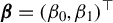
$\Gamma (Y(t),t,\boldsymbol {\beta }) = ( (Y(t) - \beta _0)\cdot (1 - t), (Y(t) - \beta _1)\cdot t )^{\top }$
 ,
$\omega (t) = \mathsf {p}_{T}(t),$
 and
${\mathcal {T}} = \{0, 1\}$
 , where
$\boldsymbol {\beta } = (\beta _{0}, \beta _{1})^{\top }$
 , the solution to (1) is
$\beta ^*_{0} = {\mathbb {E}} [Y (0)]$
 and
$\beta ^*_{1} = {\mathbb {E}}[Y (1)]$
 . ATE has been widely studied in the econometric literature (see Hahn, Reference Hahn1998; Hirano et al., Reference Hirano, Imbens and Ridder2003; Chernozhukov et al., Reference Chernozhukov, Chetverikov, Demirer, Duflo, Hansen, Newey and Robins2018, among others).
Example 2 (Quantile Treatment Effect)
When
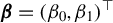
$\Gamma (Y(t),t,\boldsymbol {\beta }) = ( (\tau - \mathbb {1} \{Y(t) \leq \beta _0\})(1 - t), (\tau - \mathbb {1} \{Y(t) \leq \beta _1\})t)^{\top }$
 ,
$\omega (t) = \mathsf {p}_{T}(t),$
 and
${\mathcal {T}} = \{0, 1\}$
 , where again
$\boldsymbol {\beta } =(\beta _0,\beta _{1})^{\top }$
 , the solution to (1) is
$\beta ^*_0 = \inf \{q: \mathbb {P}(Y (0) \leq q) \geq \tau \}$
 and
$\beta ^*_{1} = \inf \{q: \mathbb {P}(Y (1) \leq q) \geq \tau \}$
 , which are the
$\tau ^{th}$
 quantiles of the potential outcomes. QTE has been studied in Chernozhukov and Hansen, Reference Chernozhukov and Hansen2005; Firpo, Reference Firpo2007; Kallus et al., Reference Kallus, Mao and Uehara2024, among others. We will revisit QTE in Sections 3.2 and 3.4 later as the most important concrete example of GTM parameters.
Example 3 (Distributional Treatment Effect (DTE))
For any
$y\in \mathbb {R}$
 , let
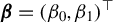
$\Gamma (Y(t),t,\boldsymbol {\beta }) = ( (\mathbb {1}\{Y(t)\leq y\} - \beta _0 )( 1- t) , (\mathbb {1}\{Y(t)\leq y\} - \beta _1) t)^{\top }$
 ,
$\omega (t) = \mathsf {p}_{T}(t)$
 , and
${\mathcal {T}} = \{0, 1\}$
 , where
$\boldsymbol {\beta } = (\beta _{0}, \beta _{1})^{\top }$
 . The solution to (1) is
$\beta ^*_{0} = \mathbb {P} (Y (0) \leq y)$
 and
$\beta ^*_{1} = \mathbb {P} (Y (1) \leq y)$
 . DTE has been studied in Chernozhukov, Fernández-Val, and Melly (Reference Chernozhukov, Fernández-Val and Melly2013) and Donald and Hsu (Reference Donald and Hsu2014), among others.
Example 4 (
$\alpha $
-Expected Shortfall)

Fix
$\alpha \in (0,1)$
 , let
${\mathcal {T}}=\{0,1\}$
 and set
$\omega (t)\equiv \mathsf {p}_T(t)$
 . Define

with
$\boldsymbol {\beta } =(\beta _0,\beta _{1})^{\top }$
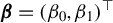 . Then the solution to (1) is given by

Thus,
$\beta _0^*$
 is the
$\alpha $
 -quantile of
$Y(1)$
 and
$\beta _1^*$
 is the associated ES. ES and related tail-risk functionals are widely used in policy learning in econometrics and related areas (see, e.g., Patton, Ziegel, and Chen, Reference Patton, Ziegel and Chen2019; Fan et al., Reference Fan, Qi and Xu2025).
Up to this point, all the examples have set
$\omega (\cdot ) \equiv \mathsf {p}_{T} (\cdot )$
 . In the next example,
$\omega (\cdot )$
 is taken as a known function of T.
Example 5 (Stochastic Intervention Effect)
The weighting function
$\omega (t)$
 can be further generalized to depend on the covariates, that is,
$\omega (t, x)$
 . When
$\omega (t, x)$
 is a known, user-specified density function of T,
$\boldsymbol {\beta }^{\ast }$
 corresponds to the stochastic (dynamical) intervention effect (Kennedy, Reference Kennedy2019).
Example 6 (Marginal Structural Models (MSMs))
In its most common formulation, MSMs (Robins et al., Reference Robins, Hernán and Brumback2000) postulate a parametric model for the marginal mean of potential outcomes:

Model (3) can be rewritten as Model (1) by letting
$\Gamma (Y (t), t, \boldsymbol {\beta }^{\ast }) = Y (t) - g (t; \boldsymbol {\beta }^{\ast })$
 . The weighting function
$\omega $
 needs to be arbitrary if (3) is taken as part of the modeling assumptions. See Section S1 of the Supplementary Material for further discussions.
If we set the weighting function
$\omega (\cdot )$
 in (1) as the product of the marginal density function of T and the Dirac delta function
$\mathsf {p}_T(\cdot )\delta _t (\cdot )$
 for each possible treatment value
$t \in {\mathcal {T}}$
 , then the target parameter
$\boldsymbol {\beta }^* \equiv \beta ^{\ast } (\cdot )\in \mathbb {R}^{\infty }$
 becomes a function of t, that is, an infinite-dimensional (
$p=\infty $
 ) parameter. In Section 4, we further develop our approach for such infinite-dimensional GTM parameters. Notably, this framework encompasses two important infinite-dimensional parameters: ADRF and QDRF.
Example 7. [Average Dose–Response Function] When
$\Gamma (Y(t),t,\beta ) = Y(t) - \beta $
 and
$\omega (\cdot ) = \mathsf {p}_T(\cdot )\delta _t (\cdot )$
 , the solution to (1) is
$\beta ^*(t) = {\mathbb {E}} [ Y(t)] $
 . The ADRF has been widely studied in the literature (see Kennedy et al., Reference Kennedy, Ma, McHugh and Small2017; Su et al., Reference Su, Ura and Zhang2019; Colangelo and Lee, Reference Colangelo and Lee2026, among others).
Example 8. [Quantile Dose–Response Function] When
$\Gamma (Y(t),t,\beta ) = \tau - \mathbb {1} \{Y(t) \leq \beta \}$
 and
$\omega (\cdot ) = \mathsf {p}_T(\cdot )\delta _t (\cdot )$
 , the solution to (1) is
$\beta ^*(t) = \inf \{q : \mathbb {P} (Y(t)\leq q) \geq \tau \}$
 , the
$\tau ^{th}$
 quantile of the potential outcome
$Y(t)$
 . The QDRF has been studied by Galvao and Wang (Reference Galvao and Wang2015) and Su et al. (Reference Su, Ura and Zhang2019).
Remark 1. Finally, though not our main focus, we note that other unknown weighting functions
$\omega $
 can also be considered. For example, when
$T \in \mathcal {T} = \mathbb {R}$
 is a continuous treatment variable with probability density function
$\mathsf {p}_T(t)$
 , let
$\Gamma (Y(t), t, \beta _0) = Y(t) + \beta _0 t$
 and
$\omega (t) = \partial _t \mathsf {p}_T(t)$
 , the derivative of
$\mathsf {p}_T(t)$
 . Under Assumption 1 and using integration by parts, the solution to (1) becomes
$\beta _0^* =\int _{{\mathcal {T}}} \partial _t {\mathbb {E}} \{\mathsf {p}_{T \mid X}^{-1}(T \mid X)Y \mid T=t\} \mathsf {p}_T^2(t) {\mathrm d} t$
 . This is the density-weighted average derivative effect (DWADE), which has been studied in recent works such as Cattaneo et al. (Reference Cattaneo, Farrell, Jansson and Masini2025) under a randomized experiment, that is, with a known propensity score function
$\mathsf {p}_{T \mid X}$
 (see Remark 6 for further discussion). Extending the analysis to observational studies is a topic worth pursuing in future work.
2.2 Review of Existing Results Based on Influence Functions
As mentioned, we take
$\omega (\cdot ) \equiv \mathsf {p}_{T} (\cdot )$
 here and in Section 3, so that
$\xi (x,t) = \mathsf {p}_{T}(t)/ \mathsf {p}_{T|X} (t|x)$
 . Before presenting our new results, we first review state-of-the-art estimators of
$\boldsymbol {\beta }^{\ast }$
 based on influence functions from the (first-order) semiparametric efficiency theory. For convenience, we define
$b_{\boldsymbol {\beta }} (x, t) := {\mathbb {E}} \{\Gamma (Y, T, \boldsymbol {\beta }) | X = x, T = t\}$
 . Since
$\Gamma (Y, T, \boldsymbol {\beta })$
 essentially plays the same role as the outcome Y in ATE, we refer to
$b_{\boldsymbol {\beta }} (\cdot ,\cdot )$
 as the generalized outcome regression model. We denote by
$\theta _{\boldsymbol {\beta }} := (\xi , b_{\boldsymbol {\beta }})$
 the collection of nuisance parameters for a fixed
$\boldsymbol {\beta }$
 . It is worth noting that
$\boldsymbol {\beta }$
 may be non-separable from the nuisance function
$b_{\boldsymbol {\beta }}$
 and can enter in a nonlinear manner. From (2) and by the law of iterated expectations,
$\boldsymbol {\beta }^{\ast }$
 solves the equation

Ai et al. (Reference Ai, Linton, Motegi and Zhang2021) developed the semiparametric efficiency theory for
$\boldsymbol {\beta }^*$
 . Since the rest of this article relies on this preliminary result, we reproduce it below in Proposition 1.
Proposition 1. Under Assumption 1, the efficient influence function (EIF) of
$\psi (\boldsymbol {\beta })$
 is

Furthermore, the EIF of
$\boldsymbol {\beta }^{\ast }$
 that solves
$\psi (\boldsymbol {\beta }) \equiv 0$
 is

For certain results in this article, we impose the following Hölder smoothness assumptions on the nuisance parameters
$\xi $
 and
$b_{\boldsymbol {\beta }}$
 .
Assumption 2.
$\xi (\cdot , \cdot )$
 and
$b_{\boldsymbol {\beta }} (\cdot , \cdot )$
 are assumed to be Hölder smooth functions with smoothness indices
$s_{1}$
 and
$s_{2}$
 respectively, for every
$\boldsymbol {\beta } \in {\mathcal {B}}$
 . We let
$s := (s_{1} + s_{2}) / 2$
 denote the average smoothness of the two nuisance parameters. The nuisance estimators
$\widehat {\xi }$
 and
$\widehat {b}_{\boldsymbol {\beta }}$
 converge to
$\xi $
 and
$b_{\boldsymbol {\beta }}$
 respectively at the minimax optimal rates (
$n^{- \frac {s_{1}}{d + 2 s_{1}}}$
 and
$n^{- \frac {s_{2}}{d + 2 s_{2}}}$
 ) in
$L_{2} (\mathbb {P})$
 -distance.
The Hölder smoothness conditions in Assumption 2 are standard for quantifying the complexity of nuisance functions in nonparametric and semiparametric theory. The stated minimax rates are attainable by classical series, sieve, and kernel estimators under appropriate choice of tuning parameters, such as the bandwidth or the number of basis functions (see, e.g., Stone, Reference Stone1982).
As noted in the Introduction, a major statistical challenge in applying
$\mathsf {IF}_{\psi }^{(1)}$
 to construct a first-order estimator of
$\boldsymbol {\beta }$
 is that the nuisance parameter
$b_{\boldsymbol {\beta }}$
 itself depends on the unknown parameter
$\boldsymbol {\beta }$
 . Directly applying Proposition 1 therefore requires estimating the entire nuisance function, meaning that
$b_{\boldsymbol {\beta }}$
 needs to be estimated for every candidate
$\boldsymbol {\beta }$
 . One simple way to bypass this difficulty is to first obtain an initial estimator
$\boldsymbol {\beta }_{\mathsf {init}}$
 close to
$\boldsymbol {\beta }^{\ast }$
 , for example, by solving the empirical version of (4) and then substitute
$b_{\boldsymbol {\beta }_{\mathsf {init}}}$
 into the influence function
$\mathsf {IF}_{\psi }^{(1)}$
 . This approach is referred to as LDML, recently developed in Kallus et al. (Reference Kallus, Mao and Uehara2024).
To formally construct this first-order estimator
$\widehat {\boldsymbol {\beta }}^{(1)}$
 , we define

where
$O'=(Y',T',X')$
 is an independent copy of
$O = (Y,T,X)$
 .
We construct the first-order estimator
$\widehat {\psi }^{(1)}(\boldsymbol {\beta })$
 of
$\psi (\boldsymbol {\beta })$
 by the following second-order U-statistic (similar construction also appeared in Tchetgen Tchetgen, Robins, and Rotnitzky, Reference Tchetgen Tchetgen, Robins and Rotnitzky2010 and Bonvini et al., Reference Bonvini, Kennedy, Ventura and Wasserman2022):

and define
$\widehat {\boldsymbol {\beta }}^{(1)}$
 as the solution to
$\widehat {\psi }^{(1)}(\boldsymbol {\beta }) \equiv 0$
 . For convenience, we assume that the nuisance estimators
$\widehat {\xi }$
 ,
$\widehat {b}_{\boldsymbol {\beta }_{\mathsf {init}}}$
 and the initial estimator
$\boldsymbol {\beta }_{\mathsf {init}}$
 of
$\boldsymbol {\beta }^*$
 are all computed using an independent separate sample of size n, referred to as the nuisance sample. The U-statistic operator
${\mathbb {U}}_{n, m}$
 , for any
$m \geq 2$
 , is taken only over the main sample throughout the article. All results are stated conditional on the nuisance sample. For brevity, we often suppress this dependence in our notation, particularly the dependence on
$\boldsymbol {\beta }_{\mathsf {init}}$
 . To improve efficiency, one can follow the standard cross-fitting procedure of Chernozhukov et al. (Reference Chernozhukov, Chetverikov, Demirer, Duflo, Hansen, Newey and Robins2018) by flipping the roles of the main and nuisance samples to construct a cross-fit version of the estimator
$\widehat {\psi }^{(1)} (\boldsymbol {\beta })$
 . However, to avoid notation clutter, we will stick to the estimator without cross-fitting.
Remark 2. In the case of a binary treatment
$T \in \{0,1\}$
 , we have
$\xi (X,T) = T/\mathbb {P}(T = 1 | X) + (1 - T)/\mathbb {P}(T = 0 | X)$
 ,
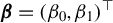
$\boldsymbol {\beta }=(\beta _0,\beta _1)^{\top }$
 and
$b_{\boldsymbol {\beta }} (X, T) = T \cdot {\mathbb {E}} \{\Gamma (Y,T,\beta _1) \mid X, T=1\} + (1 - T) \cdot {\mathbb {E}} \{\Gamma (Y,T,\beta _0) \mid X, T = 0\}$
 . The influence function of
$\mathsf {IF}_{\psi }^{(1)}(\boldsymbol {\beta })$
 then reduces to

This expression was used to construct the first-order LDML estimating equation for QTE, as proposed in Section 1.1 of Kallus et al. (Reference Kallus, Mao and Uehara2024); see Section 3.2 for a further discussion. For a continuous treatment T, the influence function leads to a second-order U-statistic estimator.
The statistical properties of
$\widehat {\boldsymbol {\beta }}^{(1)}$
 are formally stated in Proposition 2 below. This result is analogous to Theorem 1 of Kallus et al. (Reference Kallus, Mao and Uehara2024). A proof sketch is provided in Section 3.1, which also serves to motivate the introduction of our HOEs.
Proposition 2. Suppose that Assumption 1 holds and there exist three diminishing sequences
$r_{n, \xi }, r_{n, b}, r_{n, \boldsymbol {\beta }_{\mathsf {init}}}\rightarrow 0$
 as
$n \rightarrow \infty $
 such that

If we further assume that conditions (i)–(vi) of Theorem 3 in Kallus et al. (Reference Kallus, Mao and Uehara2024) hold after the substitutions
$\theta \mapsto \boldsymbol {\beta },\; \mu \mapsto b,\; U+V\mapsto \psi $
 and that
$r_{n, \xi } ( r_{n, b} + r_{n, \boldsymbol {\beta }_{\mathsf {init}}}) = o (n^{- 1 / 2})$
 , then

where
$\sigma ^{2} = \mathrm {var} (\mathsf {IF}_{\boldsymbol {\beta }^*}^{(1)})$
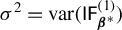 and
$\mathsf {IF}_{\boldsymbol {\beta }^*}^{(1)}$
 is the EIF of
$\boldsymbol {\beta }^*$
 defined in (5).
Proposition 2 shows that, for
$\widehat {\boldsymbol {\beta }}^{(1)}$
 to be
$n^{-1/2}$
 -consistent and asymptotically normal, the initial estimator
$\boldsymbol {\beta }_{\mathsf {init}}$
 must converge to
$\boldsymbol {\beta }^{\ast }$
 fast enough to accurately estimate the nuisance function
$b_{\boldsymbol {\beta }}$
 . If
$\boldsymbol {\beta }_{\mathsf {init}}$
 is obtained by solving the empirical version of (4) using estimated stabilized weights
$\widehat {\xi }$
 that converge to the true
$\xi $
 at rate
$r_{n,\xi }$
 , then
$r_{n,\boldsymbol {\beta }_{\mathsf {init}}} = O(r_{n,\xi })$
 . Thus, unless
$r_{n,\boldsymbol {\beta }_{\mathsf {init}}}$
 converges to zero at an even faster rate than
$r_{n,\xi }$
 (a highly unlikely scenario), we require both
$r_{n,\xi }$
 and
$r_{n,b}$
 to be
$o_{\mathbb {P}}(n^{-1/4})$
 .
Under Assumption 2, these rate conditions imply that
$\frac {2s_{1}/d}{1 + 2 s_{1}/d}> 0.5$
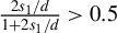 and
$\frac {s_{1}/d}{1 + 2 s_{1}/d} + \frac {s_{2}/d}{1 + 2 s_{2}/d}> 0.5$
 . In the special case
$s_{1}=s_{2}=s$
 , this further reduces to
$s/d> 0.5$
 , under which both nuisance parameters even satisfy the Donsker condition. However, inspired by the known optimal rate for ATE estimation under Hölder-type nuisance assumptions (Robins et al., Reference Robins, Li, Liu, Mukherjee, Tchetgen Tchetgen and van der Vaart2023), it is reasonable to conjecture that
$s/d \geq 0.25$
 suffices to guarantee a
$n^{-1/2}$
 -consistent estimator for finite-dimensional parameters of GTM under reasonable regularity conditions on the generalized residual function
$\Gamma $
 . The remainder of this section is devoted to constructing an HOE of
$\boldsymbol {\beta }^{\ast }$
 requiring much relaxed Hölder-type smoothness assumptions on the nuisance parameters and the initial
$\boldsymbol {\beta }_{\mathsf {init}}$
 , by leveraging the HOIF framework.
3 HIGHER-ORDER ESTIMATORS: THE FINITE-DIMENSIONAL CASE
In this section, we present our main methodological and theoretical results on new HOEs for finite-dimensional GTM parameters. We first motivate the need for HOEs beyond the first-order estimator
$\widehat {\boldsymbol {\beta }}^{(1)}$
 through a simple numerical experiment in Section 3.1, accompanied by a brief and intuitive introduction to HOIF theory. Section 3.2 then discusses how to construct HOEs for GTM parameters, and Section 3.3 studies their statistical properties. Finally, Section 3.4 specializes these general results to the QTE.
3.1 Motivation for Higher-Order Estimators: The QTE Example
Before proceeding, we provide a more technically rigorous motivation for constructing HOEs for GTMs, complementing the empirical motivation based on the simulation results in Figure 1 in the Introduction. We focus on
$\beta _{1}^{\ast }$
 , the
$\tau $
 -quantile of the potential outcome
$Y(1)$
 , which was shown to be a GTM parameter in Example 2. As discussed in Remark 2 and Proposition 2 (following Kallus et al. (Reference Kallus, Mao and Uehara2024)), we can analyze the bias of the LDML estimator
$\widehat {\beta }^{(1)}$
 by examining the bias of the first-order moment equation
$\widehat {\psi }^{(1)}(\beta _1)$
 for
$\psi (\beta _1)$
 at a given
$\beta _1$
 :

where we recall that
$\xi (x, t) = t / \mathbb {P} (T = 1 \mid X = x)$
 ,
$b_{\beta _{1}} (x, t) = t \cdot \mathbb {E} [\tau - \mathbb {1} \{Y \leq \beta _{1}\} \mid X = x, T = t]$
 , and
$\widehat {\xi }$
 and
$\widehat {b}_{\beta _{1}}$
 are their respective estimates. Recall that
$\widehat {\xi }$
 and
$\widehat {b}_{\beta _{1,\mathsf {init}}}$
 are constructed on the nuisance sample, whereas the expectation is taken with respect to the main sample. Hence, conditional on the nuisance sample,
$\widehat {\xi }$
 and
$\widehat {b}_{\beta _{1,\mathsf {init}}}$
 can be treated as fixed functions, and the bias
$\mathbb {E} [ \{\widehat {\xi } (X, T) - \xi (X, T)\} \{b_{\beta _{1}} (X, T) - \widehat {b}_{\beta _{1, \mathsf {init}}} (X, T)\} ]$
 captures only the approximation bias of these fixed estimators, not the sampling variability in the nuisance estimates.
Decomposing
$b_{\beta _{1}} - \widehat {b}_{\beta _{1, \mathsf {init}}}$
 as
$(b_{\beta _{1}} - b_{\beta _{1, \mathsf {init}}}) + (b_{\beta _{1, \mathsf {init}}} - \widehat {b}_{\beta _{1, \mathsf {init}}})$
 and applying the triangle inequality, we can bound the bias of
$\widehat {\psi }^{(1)}(\beta _1)$
 under suitable regularity conditions on
$\beta _1 \mapsto b_{\beta _1}$
 as follows:

Since
$\beta _{1, \mathsf {init}}$
 depends on
$\widehat {\xi }$
 , the bias of
$\widehat {\psi }^{(1)}(\beta _1)$
 is consequently bounded by

If
$\widehat {\xi }$
 or
$\widehat {b}_{\beta _{1, \mathsf {init}}}$
 does not converge sufficiently fast to their true values
$\xi $
 or
$b_{\beta _{1, \mathsf {init}}}$
 , the bias of
$\widehat {\psi }^{(1)} (\beta _{1})$
 might not be sufficiently small, as indicated by the bounds (7) and (8).
The HOE
$\widehat {\beta }_{1}^{(2)}$
 is motivated by the HOIF theory initially developed in Robins et al. (Reference Robins, Li, Tchetgen Tchetgen and van der Vaart2008), which is essentially a bias reduction technique. To apply the HOIF theory to estimate
$\beta _{1}^{\ast }$
 , we first fix a set of basis functions of
$(X, T)$
 of dimension k, denoted by
$\bar {\phi }_{k}$
 . Since T is binary, we have
$\bar {\phi }_{k} (x, t) = t \bar {{\mathsf {z}}}_{k} (x)$
 for some basis functions
$\bar {{\mathsf {z}}}_{k}$
 over X. Given
$\bar {\phi }_{k}$
 , we introduce the following projections of the residuals
$\widehat {\xi } - \xi $
 and
$\widehat {b}_{\beta _{1, \mathsf {init}}} - b_{\beta _{1}}$
 onto the space spanned by
$\phi _{k}$
 (defined in Section 1.3):

where
$\Sigma _{k} = \mathbb {E} \{\bar {\phi }_{k} (X, T)^{\otimes 2}\} = \mathbb {E} \{T \bar {{\mathsf {z}}}_{k} (X)^{\otimes 2}\}$
 .
Although it is generally impossible to estimate the bias of an estimator without imposing strong assumptions, the following term can be estimated unbiasedly by a second-order U-statistic computable from the data (if
$\Sigma _{k}$
 is not known, we can plug-in some estimator
$\widehat {\Sigma }_{k}$
 of
$\Sigma _{k}$
 ):

as it is a product of two expectations of random variables that can be directly evaluated from the data. The last equality follows from
$\bar {\phi }_k(x,t) = t \bar {{\mathsf {z}}}_k(x)$
 and
$\xi (x,t) = t / \mathbb {P} (T = 1 \mid X = x)$
 , which give
${\mathbb {E}} \{\xi (X,T) \bar {\phi }_k(X,T)\} = {\mathbb {E}} \{\bar {{\mathsf {z}}}_k(X)\}$
 , and by the law of iterated expectations:

Furthermore, the bias of
$\widehat {\psi }^{(1)} (\beta _{1})$
 can be decomposed as

where
$\Pi ^{\perp }$
 denotes the orthocomplement of the projection and following Robins et al. (Reference Robins, Li, Tchetgen Tchetgen and van der Vaart2008), we denote the second term in the decomposition as
$\mathrm {TB}_{\psi , k} (\beta _{1})$
 .
$\mathrm {TB}_{\psi , k} (\beta _{1})$
 is referred to as the truncation bias in Robins et al. (Reference Robins, Li, Tchetgen Tchetgen and van der Vaart2008), because it represents the remaining bias, after “truncating” the potentially infinite-dimensional residual functions
$\widehat {\xi } - \xi $
 and
$b_{\beta _{1}} - \widehat {b}_{\beta _{1, \mathsf {init}}}$
 up to a finite dimension k by the basis
$\bar {\phi }_{k}$
 . Under appropriate assumptions on
$\widehat {\xi } - \xi $
 and
$b_{\beta _{1}} - \widehat {b}_{\beta _{1, \mathsf {init}}}$
 and a suitable choice of
$\bar {\phi }_{k}$
 (to be clarified later),
$\mathrm {TB}_{\psi , k} (\beta _{1})$
 can be made negligible compared to sampling variability.
The key idea of our higher-order estimation approach is to decompose the bias of the first-order estimator
$\widehat {\psi }^{(1)} (\beta _{1})$
 of
$\psi (\beta _{1})$
 into two parts
$\mathrm {B}_{\psi , k} (\beta _{1}) + \mathrm {TB}_{\psi , k} (\beta _{1})$
 , so that
$\mathrm {B}_{\psi , k} (\beta _{1})$
 can be estimated at a sufficiently fast rate by an estimator
$\widehat {\mathrm {B}}_{\psi , k}$
 and
$\mathrm {TB}_{\psi , k} (\beta _{1})$
 is negligible. We then solve a bias-reduced estimating equation
$\widehat {\psi }^{(1)} - \widehat {\mathrm {B}}_{\psi , k}$
 (typically a U-statistic) to construct the HOE
$\widehat {\beta }_{1}^{(2)}$
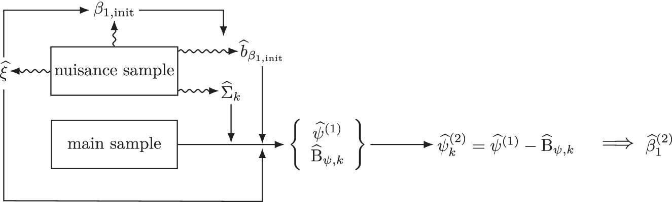
 . We summarize the construction of
$\widehat {\beta }_{1}^{(2)}$
 in Figure 2.
A schematic illustration on how to construct the higher-order estimator
$\widehat {\beta }_{1}^{(2)}$
 of
$\beta _{1}^*$
 in the example of QTE.
$\widehat {\mathrm {B}}_{\psi , k}$
 is a second-order U-statistic estimator of
$\mathrm {B}_{\psi , k}$
 .
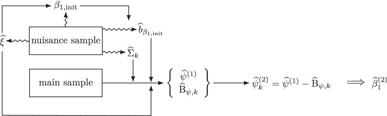
Figure 2 Long description
The flowchart begins on the left with two stacked rectangular boxes labeled nuisance sample on top and main sample on the bottom.
From the nuisance sample box, four wavy arrows point outward to different variables. One points left to xi hat. One points up to beta sub 1 comma init. One points right to b hat sub beta sub 1 comma init. One points right to Sigma hat sub k.
A solid line with arrows connects xi hat and beta sub 1 comma init to a vertical line that feeds into the main processing stream.
The main sample box has a solid horizontal arrow pointing right. This arrow is joined by vertical inputs from Sigma hat sub k and b hat sub beta sub 1 comma init.
These combined inputs lead into a set of curly brackets containing psi hat super 1 and B hat sub psi comma k.
A solid arrow points from the brackets to an equation: psi hat sub k super 2 equals psi hat super 1 minus B hat sub psi comma k.
Finally, a double-lined arrow points to the far right result: beta hat sub 1 super 2.
As mentioned in the Introduction, Figure 1 displays the histograms of different QTE estimators after centered on the true QTE value (i.e., the estimate minus the truth) in a simulation setting where nuisance estimation errors
$\|\widehat {\xi } - \xi \|_{\mathbb {P},2}$
 and
$\|\widehat {b}_{\beta _{1,\mathsf {init}}} - b_{\beta _{1,\mathsf {init}}}\|_{\mathbb {P},2}$
 are designed to be large. In the left panel, the LDML estimator exhibits a noticeable bias relative to its sampling variability. In contrast, the right panel shows that the histogram of our HOEs is much more centered around zero, indicating a negligible bias relative to its sampling variability. The variance of the HOE is only slightly larger than that of the LDML estimator. These results demonstrate that the proposed HOE can be useful not only in theory but also in practice.
3.2 Higher-Order Estimators: The General Case
In the general case, we begin by noting that the bias of the first-order estimator
$\widehat {\psi }^{(1)} (\boldsymbol {\beta })$
 for the moment equation
$\psi (\boldsymbol {\beta })$
 can also be written as the mean of a product of two nuisance estimation residuals:

To reduce this bias, we project each residual onto a size-k dictionary
$\bar {\phi }_{k} := \{\phi _{1}, \cdots , \phi _{k}\}$
 functions. Specifically, we select
$\bar {\phi }_{k} \equiv \bar {{\mathsf {z}}}_{k_{x}} \otimes \bar {{\mathsf {w}}}_{k_{t}}$
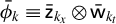 as the tensor product of a size-
$k_{x}$
 dictionary
$\bar {{\mathsf {z}}}_{k_{x}} := \{\mathsf {z}_{1}, \cdots , \mathsf {z}_{k_{x}}\}$
 over
${\mathcal {X}}$
 and a size-
$k_{t}$
 dictionary
$\bar {{\mathsf {w}}}_{k_{t}} := \{\mathsf {w}_{1}, \cdots , \mathsf {w}_{k_{t}}\}$
 over
${\mathcal {T}}$
 , as in general T is no longer binary. Using the same projection arguments as in Section 3.1, the bias decomposes as

where
$\Pi $
 denotes projection onto the span of
$\bar {\phi }_k$
 and
$\Pi ^{\perp }$
 is its orthocomplement. Moreover,

A key insight underlying the improved second-order estimator is that the bias term
$\mathrm {B}_{\psi ,k}(\boldsymbol {\beta })$
 admits an unbiased sample analog, if
$\Sigma _k$
 is known. First, by the law of iterated expectations,

Next, recall that
$\xi (X,T)=\mathsf {p}_T(T)/\mathsf {p}_{T\mid X}(T\mid X)$
 . Weighting by
$\xi $
 transforms the joint distribution of
$(X,T)$
 into the product of their marginal distributions. Indeed,

This identity is crucial: it shows that the expectation of
$\xi (X,T)\bar {\phi }_k(X,T)$
 can be estimated by averaging
$\bar {\phi }_k(X_i,T_j)$
 over independent pairs
$(X_i,T_j)$
 from the main sample. Combining these two observations, we obtain an unbiased estimator of
$\mathrm {B}_{\psi ,k}(\boldsymbol {\beta })$
 as the following third-order U-statistic:

Recall that the U-statistics operator
$\mathbb {U}_{n,3}$
 is taken over the main sample. We then construct the improved oracle second-order estimator of
$\psi (\boldsymbol {\beta })$
 as

We call
$\widetilde {\psi }_{ k}^{(2)}$
 an oracle estimator because it requires the knowledge of
$\Sigma _{k}$
 , which is generally unknown. The corresponding oracle second-order estimator
$\widetilde {\boldsymbol {\beta }}^{(2)}$
 for
$\boldsymbol {\beta }^*$
 is defined as the solution to
$\widetilde {\psi }_{k}^{(2)} (\boldsymbol {\beta }) = 0$
 . When
$\Sigma _{k}$
 is replaced by an estimator
$\widehat {\Sigma }_{k}$
 (see Remark 5) computed from the nuisance sample, we obtain the feasible estimators
$\widehat {\mathrm {B}}_{\psi , k}$
 and
$\widehat {\psi }_{k}^{(2)} (\boldsymbol {\beta }) := \widehat {\psi }^{(1)} (\boldsymbol {\beta }) - \widehat {\mathrm {B}}_{\psi , k}(\boldsymbol {\beta })$
 . The feasible estimator
$\widehat {\boldsymbol {\beta }}^{(2)}$
 for
$\boldsymbol {\beta }^*$
 is then defined as the solution to
$\widehat {\psi }_k^{(2)}(\boldsymbol {\beta }) = 0$
 .
Let
$\bar {\psi }_{k} (\boldsymbol {\beta }) := {\mathbb {E}} [\widetilde {\psi }_{k}^{(2)} (\boldsymbol {\beta })]$
 denote the truncated parameter of
$\psi (\boldsymbol {\beta }) $
 (Robins et al., Reference Robins, Li, Tchetgen Tchetgen and van der Vaart2016). The bias of the second-order estimator
$\widetilde {\psi }_{k}^{(2)} (\boldsymbol {\beta })$
 then reduces to

which can be made much smaller than the original bias. Remark 4 discusses why this yields an improved convergence rate for
$\widetilde {\psi }_{k}^{(2)} (\boldsymbol {\beta })$
 under Hölder-type assumptions in Assumption 2. Formally analyzing the statistical properties of
$\widetilde {\boldsymbol {\beta }}^{(2)}$
 and
$\widehat {\boldsymbol {\beta }}^{(2)}$
 requires a detailed examination of the impact of the initial estimator
$\boldsymbol {\beta }_{\mathsf {init}}$
 and heavy use of U-processes theory, since they are third-order Z-estimators. We will make these intuitive arguments precise in Section 3.3.
Remark 3. The initial nuisance estimators
$\widehat {\xi }$
 and
$\widehat {b}_{\boldsymbol {\beta }_{\mathsf {init}}}$
 can be obtained by any flexible method (e.g., kernel smoothing, series estimation, or machine learning) and are treated as fixed functions conditional on the nuisance sample. The dictionary
$\bar {\phi }_k$
 is introduced solely for the purpose of bias correction: we project the residual functions
$\widehat {\xi }-\xi $
 and
$b_{\boldsymbol {\beta }}-\widehat {b}_{\boldsymbol {\beta }_{\mathsf {init}}}$
 onto the linear span of
$\bar {\phi }_k$
 , and the bias correction term
$\widetilde {\mathrm {B}}_{\psi ,k}(\boldsymbol {\beta })$
 estimates the inner product of these projections. The improvement comes from choosing
$\bar {\phi }_k$
 with sufficient approximation power for these residuals; in particular, the dictionary used for bias correction should be richer than or different from any dictionary used in the initial nuisance estimation.
Remark 4. We now provide intuition for the improved convergence rate of the debiased estimator
$\widetilde {\psi }_{k}^{(2)} (\boldsymbol {\beta })$
 . For simplicity, we ignore the impact of
$\boldsymbol {\beta }_{\mathsf {init}}$
 by assuming
$\boldsymbol {\beta }_{\mathsf {init}} = \boldsymbol {\beta }$
 . Under Assumption 2 and with an appropriate choice of basis
$\bar {\phi }_{k}$
 (Belloni et al., Reference Belloni, Chernozhukov, Chetverikov and Kato2015), the truncation bias satisfies
$\mathrm {TB}_{\psi , k}(\boldsymbol {\beta }) \asymp k^{- 2 s/d}$
 , where s is the average smoothness defined in Assumption 2. The variance of
$\widetilde {\psi }_{k}^{(2)} (\boldsymbol {\beta })$
 is of order
$\frac {k}{n^{2}} + \frac {1}{n}$
 . Balancing the truncation bias against the variance by choosing
$k \asymp n^{\frac {2 d}{d + 4 s}}$
 yields

Thus, compared to the first-order estimator
$\widehat {\psi }^{(1)}$
 , the debiased estimator
$\widetilde {\psi }_k^{(2)}$
 relaxes the smoothness requirement for
$\sqrt {n}$
 -consistency. Specifically,
$\widetilde {\psi }_k^{(2)}$
 achieves the
$\sqrt {n}$
 rate whenever
$s \ge d/4$
 , whereas
$\widehat {\psi }^{(1)}$
 fails in the regime
$d/4 < s < d/2$
 (see the discussion following Proposition 2).
Remark 5. Following McGrath and Mukherjee (Reference McGrath and Mukherjee2024) and Chen et al. (Reference Chen, Liu and Mukherjee2024b), we focus on the case where
$\Sigma _{k}^{-1}$
 is known or some estimator
$\widehat {\Sigma }_{k}^{-1}$
 of
$\Sigma _{k}^{-1}$
 is sufficiently close to
$\Sigma _{k}^{-1}$
 , which generally requires extra smoothness assumptions on the marginal density
$\mathsf {p}_{X}$
 of X. How the minimax-optimal rate depends on the smoothness of
$\mathsf {p}_{X}$
 is a long-standing open problem (Richardson and Rotnitzky, Reference Richardson and Rotnitzky2014) and is beyond the scope of this article. For completeness, in Section S3 of the Supplementary Material, we derive the HOIFs of
$\psi (\boldsymbol {\beta })$
 (or more precisely, of
$\bar {\psi }_{k} (\boldsymbol {\beta }) $
 ) and construct HOEs of arbitrary order m, facilitating future work in this direction. When
$k = o (n)$
 , we briefly discuss in Section S3.1 of the Supplementary Material how to estimate
$\boldsymbol {\beta }$
 using HOEs with
$m \asymp \log n$
 without any smoothness assumption on
$\mathsf {p}_{X}$
 , where
$\Sigma _{k}$
 is estimated by its sample average estimator.
3.3 Asymptotic Properties of Higher-Order Estimators: The General Case
En route to deriving statistical properties of our proposed second-order estimators, we further require the following regularity conditions. When stating these conditions, we introduce positive and finite constants
$c_{3}, \ldots , c_{8}$
 that do not vary with n.
Assumption 3. The support
$\mathcal {T}$
 of the treatment variable T is a compact subset of
${\mathbb {R}}$
 .
Assumption 4. (i) The parameter space
${\mathcal {B}}$
 is a compact subset of
${\mathbb {R}}^{p}$
 and the true parameter
$\boldsymbol {\beta }^{*}$
 is in the interior of
${\mathcal {B}}$
 . (ii)
$\boldsymbol {\beta }^{\ast }$
 is the unique solution to the population first-order estimating equation
$\psi (\boldsymbol {\beta }) = 0$
 and for every
$\epsilon> 0$
 ,
$\inf _{\|\boldsymbol {\beta } - \boldsymbol {\beta }^{\ast }\| \geq \epsilon } \|\psi (\boldsymbol {\beta })\|> 0$
 .
Assumption 5. (i)
$\psi (\boldsymbol {\beta })$
 is differentiable with respect to
$\boldsymbol {\beta }$
 at any
$\boldsymbol {\beta } \in {\mathcal {B}}$
 ; denote its derivative with respect to
$\boldsymbol {\beta }$
 as
$\nabla _{\boldsymbol {\beta }} \psi (\boldsymbol {\beta }) \in {\mathbb {R}}^{p \times p}$
 . (ii) Each component of
$\nabla _{\boldsymbol {\beta }} \psi (\boldsymbol {\beta })$
 is continuous at
$\boldsymbol {\beta }^{\ast }$
 . (iii) The eigenvalues of
$\nabla _{\boldsymbol {\beta }} \psi (\boldsymbol {\beta }^{\ast })$
 are bounded between constants
$c_3$
 and
$c_4$
 .
Assumption 6. (i)
$\sup _{\boldsymbol {\beta } \in {\mathcal {B}}} \|b_{\boldsymbol {\beta }} (\cdot , \cdot )\|_{\infty } \lesssim 1$
 ,
$\sup _{\boldsymbol {\beta } \in {\mathcal {B}}} \|\widehat {b}_{\boldsymbol {\beta }} (\cdot , \cdot )\|_{\infty } \lesssim 1$
 and
$ \|\widehat {\xi } (\cdot , \cdot ) \|_{\infty } \lesssim 1$
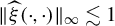 . (ii) For any
$\boldsymbol {\beta }_{1}, \boldsymbol {\beta }_{2} \in {\mathcal {B}}$
 , we have
$ \| {b}_{\boldsymbol {\beta }_{1}}(X,T)-{b}_{\boldsymbol {\beta }_{2}} (X,T) \|_{\mathbb {P},2} \lesssim \| \boldsymbol {\beta }_{1} - \boldsymbol {\beta }_{2}\|.$
 (iii) For any
$(x, t) \in {\mathcal {X}} \times {\mathcal {T}}$
 , we have
$ \ c_5 \leq \mathsf {p}_{X}(x)\leq c_6 $
 and
$ \ c_5 \leq \mathsf {p}_{T}(t)\leq c_6$
 .
Assumption 7. (i) The function class
$\left \{ \Gamma (\cdot , \cdot , \boldsymbol {\beta }): \boldsymbol {\beta } \in {\mathcal {B}} \right \}$
 is of VC type with fixed characteristic
$(A, v)$
 . (ii)
$\sup _{\boldsymbol {\beta } \in {\mathcal {B}}} \| \Gamma (\cdot ,\cdot ,\boldsymbol {\beta }) \|_{\infty } \lesssim 1$
 . (iii) There exists some constant
$\alpha _{0}\in (0,1]$
 such that, for any
$\boldsymbol {\beta }_{1}, \boldsymbol {\beta }_{2} \in {\mathcal {B}}$
 , any small
$\delta>0$
 ,
${\mathbb {E}}^{1/2} [\sup _{||\boldsymbol {\beta }_{1}-\boldsymbol {\beta }_{2}||\lesssim \delta } \left \| \Gamma (Y,T,\boldsymbol {\beta }_1)-\Gamma (Y,T,\boldsymbol {\beta }_2) \right \|^2 ]\lesssim \delta ^{\alpha _{0}}$
 .
Assumption 8. (i) For each j, the
$j^{th}$
 basis functions
$\mathsf {z}_{j}(\cdot )$
 and
$\mathsf {w}_{j}(\cdot )$
 are supported on sets of probability at most
$c_7/k_x$
 and
$c_7/k_t$
 , respectively. Let
${\mathcal {S}}_{X,j}$
 and
${\mathcal {S}}_{T,j}$
 denote the supports of
$\mathsf {z}_{j}(\cdot )$
 and
$\mathsf {w}_{j}(\cdot )$
 , respectively. (ii) At any point
$(x,t)\in {\mathcal {X}} \times {\mathcal {T}}$
 , at most
$c_8$
 elements of
$\bar {{\mathsf {z}}}_{k_{x}} (x)$
 and
$\bar {{\mathsf {w}}}_{k_{t}} (t)$
 are simultaneously nonzero. (iii) For every
$k_{x}$
 and
$k_{t}$
 , and for any unit vectors
${\boldsymbol {a}}=(a_1,\ldots ,a_{k_x})\in {\mathbb {R}}^{k_x}$
 and
${\boldsymbol {b}}=(b_1,\ldots ,b_{k_t})\in {\mathbb {R}}^{k_t}$
 , we have
${\boldsymbol {a}}^{\top }\int _{{\mathcal {S}}_{X,j}} \bar {{\mathsf {z}}}_{k_{x}} (x)\bar {{\mathsf {z}}}_{k_{x}} (x)^{\top } {\mathrm d} x {\boldsymbol {a}} \gtrsim a_j^2 $
 and
${\boldsymbol {b}}^{\top }\int _{{\mathcal {S}}_{T,j}} \bar {{\mathsf {w}}}_{k_{t}} (t) \bar {{\mathsf {w}}}_{k_{t}} (t)^{\top } {\mathrm d} t {\boldsymbol {b}} \gtrsim b_j^2$
 . (iv) There exist two sequences of constants
$\zeta _{x}(k_{x})$
 and
$\zeta _{t}(k_{t})$
 such that
$\Vert \bar {{\mathsf {w}}}_{k_{t}} (\cdot ) \Vert _{\infty } \leq \zeta _{t}(k_{t}) \lesssim \sqrt {k_t}$
 ,
$\Vert \bar {{\mathsf {z}}}_{k_{x}} (\cdot ) \Vert _{\infty } \leq \zeta _{x}(k_{x}) \lesssim \sqrt {k_x}$
 , and
$\zeta (k):= \zeta _{x}(k_{x})\zeta _{t}(k_{t})$
 . (v) The dimension
$k=k_x k_t$
 satisfies
$k \to \infty $
 and
$k = o (n^2)$
 as
$n \to \infty $
 .
Assumption 3 requires that the treatment T be bounded. This condition is imposed to simplify the analysis, as most existing technical tools for U-statistics and U-processes require the U-statistic kernel to be bounded. We expect that it could be weakened to light-tailed conditions (Chakrabortty and Kuchibhotla, Reference Chakrabortty and Kuchibhotla2025), but this is not the main focus of our article. Assumptions 4 and 5 are standard identification and regularity conditions for Z-estimators. Assumption 6 imposes sufficient regularity conditions on the nuisance functions and their estimators. In particular, Assumption 6(iii), together with Assumption 1(ii), implies that
$\xi (\cdot ,\cdot )$
 is bounded away from zero and infinity, which is commonly required in the existing literature; see Ai et al. (Reference Ai, Linton, Motegi and Zhang2021) and Kennedy et al. (Reference Kennedy, Ma, McHugh and Small2017), among others.
Assumption 7(i) is a high-level complexity condition on the generalized residual function that defines GTM treatment effect parameters in (1). In applications, this assumption shall be verified case-by-case. Assumptions 7(ii) and (iii) control the envelope functions, a standard requirement in
$M/Z$
 -estimation when the criterion is non-smooth (see, e.g., Chen et al., Reference Chen, Linton and Van Keilegom2003; Ai et al., Reference Ai, Linton, Motegi and Zhang2021). Notably, Assumption 7(iii) is weaker than the Lipschitz continuity condition and accommodates various continuous and discontinuous functions. Fortunately, in various examples, these assumptions are straightforward to verify. In Section S2 of the Supplementary Material, we show that they hold for both ATE and QTE from Examples 1 and 2.
Assumptions 8(i) and (ii) ensure control over the sup norm of series projection estimators, which are essential for analyzing the U-process and establishing variance bounds. These assumptions are satisfied by many commonly used sieve bases, including Cohen–Daubechies–Vial wavelet series, B-splines and local polynomial partition series; see Belloni et al., Reference Belloni, Chernozhukov, Chetverikov and Kato2015; Liu et al., Reference Liu, Mukherjee, Newey and Robins2017; Cattaneo, Farrell, and Feng, Reference Cattaneo, Farrell and Feng2020 for detailed discussions. Assumption 8(iii) imposes a mild local non-collinearity requirement on the basis functions and is verified by the basis functions mentioned above. This condition is also adopted in Cattaneo et al. (Reference Cattaneo, Farrell and Feng2020). Assumption 8(iv) is standard in the nonparametric regression literature and is verified for the basis functions mentioned above. Assumption 8(v) restricts the basis dimension k from growing too fast (slower than
$n^{2}$
 ), a necessary condition to achieve asymptotic normality of the estimators.
We now establish the consistency and convergence rate of the oracle second-order estimator
$\widetilde {\boldsymbol {\beta }}^{(2)}$
 .
Theorem 1. Suppose that Assumptions 1 and 3–8 hold. Let
$\widetilde {r}_{n,\boldsymbol {\beta }} \to 0$
 be a diminishing sequence such that

where
$\Pi ^{\perp }[f \mid \bar {\phi }_{k}]$
 denotes the orthocomplement of the projection of f onto the linear span of
$\bar {\phi }_{k}$
 (see Section 1.3). Then
$\widetilde {\boldsymbol {\beta }}^{(2)}$
 is consistent and satisfies
${\mathbb {E}}[\|\widetilde {\boldsymbol {\beta }}^{(2)} - \boldsymbol {\beta }^{*}\|] \lesssim \widetilde {r}_{n,\boldsymbol {\beta }}$
 .
The proof of Theorem 1 is presented in Section S7.1 of the Supplementary Material. The convergence rate
$\widetilde {r}_{n,\boldsymbol {\beta }}$
 comprises two components: the first term captures variance, and the second term represents the bias arising from approximating the residuals of the estimated and true nuisance parameters using the basis
$\bar {\phi }_{k}$
 .
The next result characterizes the asymptotic distribution of
$\widetilde {\boldsymbol {\beta }}^{(2)}$
 .
Theorem 2. Suppose Assumptions 1 and 3–8 hold. Further, assume
$\widetilde {r}_{n,\boldsymbol {\beta }}^{\alpha _{0}} \log n \rightarrow 0$
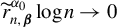 , where
$\alpha _{0}$
 is the constant from Assumption 7, and that

Then

where
$V_1(\boldsymbol {\beta })$
 and
$V_2(\boldsymbol {\beta })$
 are defined in (S7.12) and (S7.13) in Section S7.3 of the Supplementary Material. In particular, the asymptotic variance depends on the relative scaling between k and n:
$V_2(\boldsymbol {\beta }^{\ast })=0$
 when
$k\ll n$
 , while
$V_1(\boldsymbol {\beta }^{\ast })=0$
 when
$k\gg n$
 . Consequently,
-
(i) if $k \ll n$
, then $$ \begin{align*} \sqrt{n} (\widetilde{\boldsymbol{\beta}}^{(2)} -\boldsymbol{\beta}^{*}) & \stackrel{d}{\to} N \left( 0, \{\nabla_{\boldsymbol{\beta}}\psi (\boldsymbol{\beta}^{*})\}^{-1}V_1 (\boldsymbol{\beta}^{\ast}) \{\nabla_{\boldsymbol{\beta}}^{\top}\psi (\boldsymbol{\beta}^{*})\}^{-1} \right); \end{align*} $$
-
(ii) if $k \gg n$
(recall Assumption 8 requires
$k = o (n^{2})$
), then $$ \begin{align*} \frac{n}{\sqrt{k}} (\widetilde{\boldsymbol{\beta}}^{(2)} -\boldsymbol{\beta}^{*}) & \stackrel{d}{\to} N \left(0, \{\nabla_{\boldsymbol{\beta}}\psi (\boldsymbol{\beta}^{*})\}^{-1} \frac{1}{2} V_2 (\boldsymbol{\beta}^{\ast}) \{\nabla_{\boldsymbol{\beta}}^{\top}\psi (\boldsymbol{\beta}^{*})\}^{-1} \right); \end{align*} $$
-
(iii) and if $k / n \rightarrow \tau $
, for some
$\tau \in (0, \infty )$
, $$ \begin{align*} &\sqrt{n} (\widetilde{\boldsymbol{\beta}}^{(2)} -\boldsymbol{\beta}^{*}) \stackrel{d}{\to} \\&\quad N\left(0, (1+\tau) \{\nabla_{\boldsymbol{\beta}}\psi (\boldsymbol{\beta}^{*})\}^{-1} \left\{ V_{1} ( \boldsymbol{\beta}^{\ast} ) + \frac{1}{2} V_2 ( \boldsymbol{\beta}^{\ast} ) \right\} \{\nabla_{\boldsymbol{\beta}}^{\top}\psi (\boldsymbol{\beta}^{*})\}^{-1} \right). \end{align*} $$


The complete proof of Theorem 2 is presented in Section S7.3 of the Supplementary Material. We provide a proof sketch as follows. We begin by expanding
$\psi (\boldsymbol {\beta }^{*})$
 around
$\widetilde {\boldsymbol {\beta }}^{(2)}$
 :

where
$\boldsymbol {\beta }^{\dagger }$
 lies between
$\boldsymbol {\beta }^{*}$
 and
$\widetilde {\boldsymbol {\beta }}^{(2)}$
 . Next, we decompose
$\psi (\widetilde {\boldsymbol {\beta }}^{(2)})$
 as follows:

Term
$A_n$
 is bias-related and is
$o_{\mathbb {P}}(1)$
 under Condition (11). Term
$B_n$
 is a centered U-statistic, determining the asymptotic distribution of
$\widetilde {\boldsymbol {\beta }}^{(2)}$
 . Its asymptotic normality follows from the classical martingale CLT (Bhattacharya and Ghosh, Reference Bhattacharya and Ghosh1992). Since the kernel of this U-statistic depends on k, the linear component in the Hoeffding decomposition does not always dominate and thus the order of its asymptotic variance depends on the scaling between n and k, split into three different regimes as indicated in Theorem 2. The main technical challenge lies in analyzing the U-process term
$C_n$
 , indexed by
$\widetilde {\boldsymbol {\beta }}^{(2)}$
 and defined over a function class changing with the sample size n. Existing U-process maximal inequalities, such as those of Chen and Kato (Reference Chen and Kato2020), are conservative for our setting. To address this, we establish a refined local maximal inequality in Section S6.2 of the Supplementary Material.
Remark 6. Edgeworth expansions offer a different notion of optimality when non-asymptotic or finite sample performance is of concern. Cattaneo et al. (Reference Cattaneo, Farrell, Jansson and Masini2025) study inference for the DWADE parameter
$\beta ^{\ast }_0$
 (see Remark 1) under a randomized experiment, that is, the propensity score
$\mathsf {p}_{T|X}$
 is known, using a kernel-based estimator
$\widehat {\beta }_0$
 . Their estimator is a second-order U-statistic with Hoeffding decomposition
$\widehat {\beta }_0-\beta ^{\ast }_0 = \bar {L} + \bar {Q}$
 , where
$\bar {L}$
 and
$\bar {Q}$
 are the linear and quadratic terms, respectively. Classical asymptotics impose bandwidth conditions that make
$\bar {Q}$
 negligible, yielding an asymptotic linear representation. With smaller bandwidths,
$\bar {Q}$
 becomes non-negligible, leading to a quadratic approximation where
$\mathbb {V}[\widehat {\beta }_0] = \mathbb {V}[\bar {L}] + \mathbb {V}[\bar {Q}]$
 and
$\mathbb {V}[\widehat {\beta }_0]^{-1/2}(\widehat {\beta }_0-\beta ^{\ast }_0) \overset {d}{\to } N(0,1)$
 . Using Edgeworth expansions, they derive refined distributional approximations that improve finite-sample confidence interval coverage.
Our estimator
$\widehat {\psi }^{(2)}_k$
 of the estimating equation is also a U-statistic whose asymptotic distribution depends on quadratic terms when
$k \gtrsim n$
 . However, the goal of Cattaneo et al. (Reference Cattaneo, Farrell, Jansson and Masini2025) is inference refinement (improving finite-sample coverage), while ours is bias correction to achieve rate-optimal estimation under low smoothness conditions. In future work, we can also consider such more refined higher-order distributional approximation if concerned about the finite-sample performance beyond the asymptotic distribution results in Theorem 2.
We next derive the convergence rate of the feasible estimator
$\widehat {\boldsymbol {\beta }}^{(2)}$
 . To this end, we need the following assumption on
$\widehat {\Sigma }_{k}$
 .
Assumption 9. We assume that the estimator
$\widehat {\Sigma }_{k}$
 of
$\Sigma _{k}$
 satisfies the following condition:

Assumption 9 ensures that estimating
$\Sigma _{k}$
 by
$\widehat {\Sigma }_{k}$
 does not introduce excessive bias. When
$\boldsymbol {\beta }_{\mathsf {init}}$
 is estimated using only
$\widehat {\xi }$
 , we have
$\Vert \boldsymbol {\beta }_{\mathsf {init}} - \boldsymbol {\beta }^{\ast } \Vert \lesssim \Vert \widehat {\xi } - \xi \Vert _{\mathbb {P},2}$
 . Then the condition in Assumption 9 reduces to

Under Assumption 2, the first two terms satisfy
$\Vert \widehat {\xi } - \xi \Vert _{\mathbb {P},2}^{2} \lesssim n^{- \frac { 2s_{1} }{d + 2 s_{1}}}$
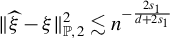 and
$\Vert \widehat {\xi } - \xi \Vert _{\mathbb {P},2} \cdot \Vert \widehat {b}_{\boldsymbol {\beta }_{\mathsf {init}}} - b_{\boldsymbol {\beta }_{\mathsf {init}}} \Vert _{\mathbb {P},2} \lesssim n^{- \frac {s_{1}}{d + 2 s_{1}} - \frac {s_{2}}{d + 2 s_{2}}}$
 . Consequently, (12) requires

which holds if the joint density
$\mathsf {p}_{X, T} (\cdot , \cdot )$
 is sufficiently smooth. Similar assumptions appear in most recent papers related to HOIF frameworks (Bonvini and Kennedy, Reference Bonvini and Kennedy2022; Kennedy et al., Reference Kennedy, Balakrishnan, Robins and Wasserman2024; McGrath and Mukherjee, Reference McGrath and Mukherjee2024) and can be relaxed using diverging-order U-statistic estimators, as detailed in Section S3 of the Supplementary Material following Liu et al. (Reference Liu, Mukherjee, Newey and Robins2017) or Robins et al. (Reference Robins, Li, Liu, Mukherjee, Tchetgen Tchetgen and van der Vaart2023).
Theorem 3 below establishes the convergence rate of the feasible estimator
$\widehat {\boldsymbol {\beta }}^{(2)}$
 using Theorem 1 together with Assumption 9. A proof is provided in Section S7.2 of the Supplementary Material.
Theorem 3. Suppose that for some constant
$c>0$
 ,
$ \Vert {\mathbb {E}} [ \widehat {\psi }^{(2)}_{k}(\boldsymbol {\beta }_1) ] - {\mathbb {E}} [ \widehat {\psi }^{(2)}_{k}(\boldsymbol {\beta }_2) ] \Vert \geq c \|\boldsymbol {\beta }_1 - \boldsymbol {\beta }_2\| .$
 Under the assumptions of Theorem 1, we have

If we further impose Assumption 9, then
${\mathbb {E}}[\Vert \widehat {\boldsymbol {\beta }}^{(2)} - \boldsymbol {\beta }^{\ast } \Vert ] \lesssim \widetilde {r}_{n,\boldsymbol {\beta }}$
 .
The final result in this section characterizes the asymptotic normality of the feasible second-order estimator
$\widehat {\boldsymbol {\beta }}^{(2)}$
 , which is a direct consequence of Theorem 2 and Assumption 9.
Theorem 4. Under the assumptions of Theorem 2, together with Assumption 9, all conclusions in Theorem 2 continue to hold for
$\widehat {\boldsymbol {\beta }}^{(2)}$
 .
Remark 7. We briefly discuss how the rate of the initial estimator
$\boldsymbol {\beta }_{\mathsf {init}}$
 impacts the results in this section. Condition (11) in Theorem 2 specifies the approximation power of
$\bar {\phi }_{k}$
 for the residuals between estimated and true nuisance parameters. Suppose that
$b_{\boldsymbol {\beta }}$
 is differentiable with respect to
$\boldsymbol {\beta }$
 . It is natural to assume that the second-order estimator is at least as close to the truth as the sub-optimal initial estimator, that is,
$\widetilde {r}_{n,\boldsymbol {\beta }} \lesssim \|\boldsymbol {\beta }_{\mathsf {init}} - \boldsymbol {\beta }^{\ast }\|$
 . Under this assumption, using the triangle inequality and a mean-value expansion in
$\boldsymbol {\beta }$
 , we can decompose the left-hand side of condition (11) as

Here,
$\mathcal {N}:= \{ \boldsymbol {\beta }: \|\boldsymbol {\beta }-\boldsymbol {\beta }^{*}\| \lesssim \|\boldsymbol {\beta }_{\mathsf {init}}-\boldsymbol {\beta }^{*}\| \}$
 , which contains all line segments between
$\boldsymbol {\beta }_{\mathsf {init}}$
 and any
$\boldsymbol {\beta }$
 with
$\|\boldsymbol {\beta }-\boldsymbol {\beta }^{*}\|\le \widetilde r_{n,\boldsymbol {\beta }}$
 . The expression (13) will be used in Section 3.4 to further clarify the rate requirement for
$\boldsymbol {\beta }_{\mathsf {init}}$
 in QTE with binary treatment.
Remark 8. As suggested by a referee, the econometrics literature contains several related proposals for bias correction in two-step semiparametric settings, including jackknife- and bootstrap-based methods (Cattaneo and Jansson, Reference Cattaneo and Jansson2018; Cattaneo et al., Reference Cattaneo, Jansson and Ma2019). In Section S5 of the Supplementary Material, we use the ATE as a concrete example to compare our approach with these alternatives. All three methods address the problem that first-stage nuisance estimation can bias the second-stage estimator. However, the sources of bias and the correction mechanisms differ. Cattaneo et al. (Reference Cattaneo, Jansson and Ma2019) and Cattaneo and Jansson (Reference Cattaneo and Jansson2018) aim to estimate the estimating equation
$\psi (\boldsymbol {\beta })$
 itself, with nuisance functions estimated by linear regression and kernel methods, respectively. The resulting estimator is affected by leave-in bias due to the reuse of the same sample in both steps, particularly when the covariate dimension is large or the bandwidth is small. By contrast, we use sample splitting and focus on estimating the approximation bias defined in (9). Our construction accommodates generic nuisance learners, such as logistic regression, random forests, or neural networks, because we use linear approximation only for the nuisance estimation residuals
$\widehat {\xi }-\xi $
 and
$\widehat {b}_{\boldsymbol {\beta }_{\mathsf {init}}}-b_{\boldsymbol {\beta }}$
 , although to obtain sharp theoretical results, we need to impose certain smoothness assumptions on
$\widehat {\xi } - \xi $
 and
$\widehat {b}_{\boldsymbol {\beta }_{\mathsf {init}}}-b_{\boldsymbol {\beta }}$
 (see Assumption 2).
Despite these differences, there are important connections. Specifically, we show that, as Cattaneo et al. (Reference Cattaneo, Jansson and Ma2019) impose (approximately) linear assumptions on the nuisance functions whereas we do so only for the residuals of the nuisance estimates, both our target parameter and that of Cattaneo et al. (Reference Cattaneo, Jansson and Ma2019) reduce to a bilinear functional (Robins et al., Reference Robins, Sued, Lei-Gomez and Rotnitzky2007; Bruns-Smith et al., Reference Bruns-Smith, Dukes, Feller and Ogburn2026) of the form
$\mathrm {B}_{\psi ,k} (\boldsymbol {\beta })$
 defined in (10). We show that the jackknife- and bootstrap-based (under some assumption on the scaling between k and n) bias-corrected estimators are, respectively, exactly equivalent and asymptotically equivalent to our second-order U-statistic estimator
$\widetilde {\mathrm {B}}_{\psi ,k}(\boldsymbol {\beta })$
 of
$\mathrm {B}_{\psi ,k}(\boldsymbol {\beta })$
 . Moreover, the HOIF framework provides a systematic way to construct higher-order U-statistic estimators even when
$\Sigma _k$
 is unknown (see Section S3 of the Supplementary Material), which we believe can also motivate similar higher-order jackknife- or bootstrap-based bias reduction methods (Koltchinskii, Reference Koltchinskii2022).
Remark 9. As also noted by one referee, both Cavaliere et al. (Reference Cavaliere, Gonçalves, Nielsen and Zanelli2024) and our article study settings where a non-negligible asymptotic bias affects the limiting distribution. However, the way how bias is handled differs. Cavaliere et al. (Reference Cavaliere, Gonçalves, Nielsen and Zanelli2024) consider statistics whose limiting distribution takes the form
$T_n = \sqrt {n}(\widehat {\theta }_n - \theta ) \stackrel {d}{\to } B_n + Z_1$
 , where
$Z_1$
 is centered normal and
$B_n$
 is a non-vanishing asymptotic bias. They construct a bootstrap analog
$T_n^* := \sqrt {n}(\widehat {\theta }_n^* - \widehat {\theta }_n)$
 , where
$\widehat {\theta }_n^*$
 is a bootstrap version of
$\widehat {\theta }_n$
 , such that
$T_n^* - \widehat {B}_n \stackrel {d^*}{\to } Z_1$
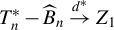 , with
$\widehat {B}_n$
 a bootstrap-based estimator of
$B_n$
 . When the bootstrap fails to replicate the bias, that is,
$\widehat {B}_n - B_n$
 does not converge to zero but converges in distribution to a zero-mean random variable, the standard bootstrap p-value

is no longer asymptotically uniform. Instead, its limiting distribution converges to a distribution H that depends on the joint limiting distribution of
$(T_n - \widehat {B}_n, T_n^* - \widehat {B}_n)$
 but not on the unknown bias
$B_n$
 itself. The key insight of Cavaliere et al. (Reference Cavaliere, Gonçalves, Nielsen and Zanelli2024) is to apply a prepivoting transformation:
$H(\widehat {p}_n)$
 is asymptotically uniform. Since H is unknown, they estimate it via a double bootstrap to obtain
$\widehat {H}_n$
 , and output the corrected p-value
$\widetilde {p}_n := \widehat {H}_n(\widehat {p}_n)$
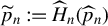 . Therefore, their procedure does not directly estimate or remove the bias
$B_n$
 ; instead, it bypasses the bias by transforming the bootstrap p-value and estimates the distribution function H.
In contrast, our approach directly estimates the bias itself. As shown in Section 3.2, we further decompose the first-order bias
$ {\mathbb {E}} [\{\widehat {\xi } (X, T) - \xi (X, T)\} \{b_{\boldsymbol {\beta }} (X, T) - \widehat {b}_{\boldsymbol {\beta }_{\mathsf {init}}} (X, T)\}]$
 into a leading bias component
$\mathrm {B}_{\psi ,k}(\boldsymbol {\beta })$
 and a truncation bias
$\mathrm {TB}_{\psi ,k}(\boldsymbol {\beta })$
 by projecting the residuals of the estimated nuisance functions onto a sieve basis
$\bar {\phi }_k$
 . The leading bias
$\mathrm {B}_{\psi ,k}(\boldsymbol {\beta })$
 is then unbiasedly estimated by a U-statistic-based correction term
$\widetilde {\mathrm {B}}_{\psi ,k}(\boldsymbol {\beta })$
 when
$\Sigma _k$
 is known (see Section 3.2). Subtracting this correction term from the first-order estimating equation yields a bias-corrected estimator
$\widehat {\boldsymbol {\beta }}^{(2)}$
 that achieves
$\sqrt {n}$
 -consistency under weaker smoothness conditions than first-order methods (see Theorem 5 and the discussion in Section 3.4).
3.4 Application: QTE with a Binary Treatment over Hölder Smoothness Classes
In this section, we revisit Section 3.1 and specialize the general results from Theorem 1 to Theorem 4 to the QTE setting with binary treatment
$T \in \{0,1\}$
 (see Example 2). To keep the exposition simple, we take the target parameter
$\beta _1^*$
 to be the
$\tau ^{th}$
 quantile of the potential outcome
$Y(1)$
 , that is,
$\beta _1^* = \inf \{q: \mathbb {P}(Y (1) \leq q) \geq \tau \}$
 . Under Assumption 1,
$\beta _1^*$
 is identified as the unique solution to

This example fits into our framework with the following correspondences:

In the QTE setting, several general regularity conditions for GTMs from Section 3.3 (Assumptions 2–7) can be simplified. In particular, Assumption 3 holds automatically because T is binary. Assumption 7 also holds for QTE under the regularity conditions stated below (see Section S2 of the Supplementary Material for verification details). To make this section self-contained, we therefore omit Assumptions 3 and 7 and restate the remaining relevant conditions as follows.
Assumption 10. (i) The parameter space
${\mathcal {B}}$
 is compact and
$\beta _1^*$
 lies in its interior; (ii)
$\beta ^{\ast }_1$
 is the unique solution to
$\psi (\beta _1)= 0$
 , and for every
$\epsilon> 0$
 ,
$\inf _{|\beta _1 - \beta _1^{\ast }| \geq \epsilon } |\psi (\beta _1)|> 0$
 ; and (iii)
$\psi (\cdot )$
 continuously differentiable on
${\mathcal {B}}$
 and its derivative function satisfies
$\nabla _{\beta _1} \psi (\beta ^{\ast }_1)> 0$
 .
Assumption 11. (i)
$\sup _{\beta _1 \in {\mathcal {B}}} \|\widehat {b}_{\beta _1} (\cdot , 1)\|_{\infty } \lesssim 1$
 ; (ii)
${\mathbb {P}} ( Y \le \beta _1| X = x, T = 1)$
 is Lipschitz continuous in
$\beta _1$
 ; and (iii) for all
$x \in {\mathcal {X}} $
 ,
$ \ c_5 \leq \mathsf {p}_{X}(x)\leq c_6$
 .
Assumption 12.
$\xi (\cdot , 1)$
 and
$\mathsf {p}_{Y|X,T} (\beta _1|\cdot , T=1)$
 are Hölder smooth with indices
$s_{1}$
 and
$s_{2}$
 , respectively, for every
$\beta _1 \in {\mathcal {B}}$
 . Let
$s = (s_1 + s_2)/2$
 denote the average smoothness. The nuisance estimators
$\widehat {\xi }$
 and
$\widehat {b}_{\beta _1}$
 converge to
$\xi $
 and
$b_{\beta _1}$
 at the minimax optimal rates (
$n^{- \frac {s_{1}}{d + 2 s_{1}}}$
 and
$n^{- \frac {s_{2}}{d + 2 s_{2}}}$
 ) in
$L_{2} (\mathbb {P})$
 . Moreover, we assume that
$\widehat {\xi }$
 and
$\widehat {b}_{\beta _{1,\mathsf {init}}}$
 belong to Hölder smoothness classes with smoothness indices
$s_{1}> 0$
 and
$s_{2}> 0$
 , respectively.
Theorem 5. For the QTE parameter
$\beta _1^* = \inf \{q: \mathbb {P}(Y (1) \leq q) \geq \tau \}$
 , suppose that Assumptions 1 and 8–12 hold. Then
-
(i) if $s / d> 1 / 4$
and
$k = o (n)$
, $$ \begin{align*} \sqrt{n} (\widehat{\beta}^{(2)}_1 - \beta^{\ast}_1) \overset{d}{\rightarrow} N \left( 0, \{\nabla_{\beta_1} \psi (\beta^{\ast}_1)\}^{-1} V_{1} (\beta^{\ast}_1) \{\nabla_{\beta_1}^{\top} \psi (\beta^{\ast}_1)\}^{-1} \right); \end{align*} $$
-
(ii) if $0 < s / d \leq 1 / 4$
and
$k \asymp n^{\frac {2}{1 + 4 s / d}}$
, $$ \begin{align*} {\mathbb{E}}^{1 / 2} [|\widehat{\beta}^{(2)}_1 - \beta^{\ast}_1|^{2}] \lesssim n^{- \frac{4 s / d}{1 + 4 s / d}}. \end{align*} $$





The convergence rates for QTE in Theorem 5 match those for ATE established in Robins et al. (Reference Robins, Li, Tchetgen Tchetgen and van der Vaart2016), which shows that these rates are minimax optimal for ATE. The proof of Theorem 5 is straightforward and proceeds as follows. Under the assumptions of Theorem 5 with an appropriate choice of basis
$\bar {\phi }_{k}$
 , we have

because the Hölder-
$s_2$
 smoothness of
$\mathsf {p}_{Y|X,T}(\beta _1 \mid \cdot , T=1)$
 implies that
$b_{\beta _1}(\cdot ,1)$
 is also Hölder-
$s_2$
 smooth for any
$\beta _1 \in {\mathcal {B}}$
 . Furthermore, a direct calculation shows that
$\nabla _{\beta _1} b_{\beta _1} (\cdot , 1) = - \mathsf {p}_{Y|X,T}(\beta _1 |\cdot , T = 1 ) $
 , which is also Hölder-
$s_{2}$
 smooth for any
$\beta _1 \in {\mathcal {B}}$
 . Combining these results with (13), the bias of
$\widehat {\beta }^{(2)}_1$
 is bounded above by

Therefore, somewhat surprisingly, the HOE imposes no rate requirement on
$\beta _{1,\mathsf {init}}$
 , as long as
$\beta _{1,\mathsf {init}}$
 is bounded. This stands in contrast to the first-order LDML estimator, which, as discussed following Proposition 2, requires
$s_1/d> 1/2$
 . We summarize these comparisons in Table 1.
Comparison of smoothness and initial estimator rate conditions for
$\sqrt {n}$
 -consistent estimation of the QTE parameter
$\beta _1^* = \inf \{q: \mathbb {P}(Y(1) \leq q) \geq \tau \}$
 .
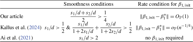
Table 1 Long description
The table consists of three columns: Source, Smoothness conditions, and Rate condition for beta sub 1 comma init.
* Row 1: Our article. Smoothness condition is the fraction with numerator s sub 1 all over d plus s sub 2 all over d all over 2 is greater than 1 fourth. Rate condition is the norm of beta sub 1 comma init minus beta super star sub 1 equals O sub P (1).
* Row 2: Kallus et al. 2024. Smoothness conditions are s sub 1 all over d is greater than 1 half and the fraction s sub 1 all over d all over 1 plus 2 s sub 1 all over d plus the fraction s sub 2 all over d all over 1 plus 2 s sub 2 all over d is greater than 1 half. Rate condition is the norm of beta sub 1 comma init minus beta super star sub 1 equals o sub P (n to the minus 1 fourth power).
* Row 3: Ai et al. 2021. Smoothness condition is s sub 1 all over d is greater than 2. Rate condition states no beta sub 1 comma init required.
Note: Here,
$s_1$
 denotes the Hölder smoothness index of the propensity score
$\xi (\cdot , 1) = 1/\mathbb {P}(T=1 \mid X = \cdot )$
 , and
$s_2$
 denotes the Hölder smoothness index of the conditional outcome density
$\mathsf {p}_{Y|X,T}(y \mid \cdot , T=t)$
 for every y.
Remark 10. For ATE in Example 1, a direct calculation yields
$b_{\boldsymbol {\beta }}(x,t) = ( ({\mathbb {E}}(Y | X = x, T = 0 ) - \beta _0)\cdot (1-t), ( {\mathbb {E}}(Y |X = x, T = 1 ) - \beta _1)\cdot t )^{\top }$
 and
$\nabla _{\boldsymbol {\beta }}b_{\boldsymbol {\beta }} (x,t) = \text {diag}(1-t, t)$
 . Each component of
$\nabla _{\boldsymbol {\beta }}b_{\boldsymbol {\beta }}$
 is infinitely smooth. As a result, condition (11) imposes no further convergence rate requirements on the initial estimator
$\boldsymbol {\beta }_{\mathsf {init}}$
 of
$\boldsymbol {\beta }^{\ast }$
 .
4 HIGHER-ORDER ESTIMATORS: TOWARD INFINITE-DIMENSIONAL PARAMETERS
For continuous or high-dimensional treatments (Su et al., Reference Su, Ura and Zhang2019), fixed-dimensional parameters in (1) are often inadequate. Motivated by Bonvini and Kennedy (Reference Bonvini and Kennedy2022) and Colangelo and Lee (Reference Colangelo and Lee2026), we extend our framework to infinite-dimensional GTMs by setting
$\omega (\cdot ) \equiv \mathsf {p}_T(\cdot )\delta _t(\cdot )$
 and letting
$p \to \infty $
 in (1). One purpose of this section is to further advocate the fruitful philosophy of turning an infinite-dimensional problem into a finite but diverging-dimensional functional estimation problem (Kennedy et al., Reference Kennedy, Balakrishnan, Robins and Wasserman2024). For notational convenience, we denote the infinite-dimensional GTM parameter as
$\beta _t^* \equiv \beta ^*(t): {\mathcal {T}} \to {\mathbb {R}}$
 , a function of the treatment value
$T=t$
 . Then
$\beta _t^*$
 solves

Under Assumption 1,
$\beta ^{\ast }_{t}$
 is identified as the solution to:

where
$\xi (x,t) = \mathsf {p}_T(t)/\mathsf {p}_{T|X}(t \mid x)$
 . Here,
$\Gamma : {\mathcal {Y}} \times {\mathcal {T}} \times {\mathcal {B}} \rightarrow {\mathbb {R}}$
 is a known one-dimensional generalized residual function. To simplify notation, we maintain the conventions of Section 2: for any
$\beta \in {\mathcal {B}}$
 , we define
$b_{\beta }(x,t) = {\mathbb {E}} \{\Gamma (Y, T, \beta ) \mid X = x, T=t\}$
 . It is worth noting that in this section we are interested in estimating the GTM parameter at some fixed treatment value
$T = t$
 .
4.1 Higher-Order Estimators for Infinite-Dimensional Parameters
Since the Dirac delta function
$\delta _{t} (\cdot )$
 cannot be evaluated in practice, we approximate it with a kernel function, following Bonvini and Kennedy (Reference Bonvini and Kennedy2022); see Remark 12 for details. Let
$K (\cdot )$
 be a base kernel function and define

We assume that the kernel
$K(\cdot )$
 satisfies the following condition, which is also imposed by Bonvini and Kennedy (Reference Bonvini and Kennedy2022).
Assumption 13.
$K (\cdot ): {\mathcal {T}} \rightarrow {\mathbb {R}} $
 is a uniformly bounded kernel function of order
$\alpha _1 \wedge \alpha _2$
 , where
$\alpha _1,\alpha _2$
 are positive integers specified in Assumption 15. It satisfies
$\int _{{\mathcal {T}}} K (u) {\mathrm d} u = 1$
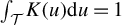 ,
$\int _{{\mathcal {T}}} u^{i}K (u) {\mathrm d} u = 0$
 for
$i=1,\ldots , \alpha _1 \wedge \alpha _2-1$
 , and
$\int _{{\mathcal {T}}} u^{\alpha _1 \wedge \alpha _2} K (u) {\mathrm d} u =: \kappa _{\alpha _1 \wedge \alpha _2,1} \neq 0$
 . Moreover,
$g(x) \in (\underline {c}_{g}, \bar {c}_g)$
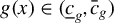 for any x and h, where
$0 < \underline {c}_g < \bar {c}_g < \infty $
 are two universal constants.
Intuitively,
$K_{t, h} (\cdot )\to \delta _{t} (\cdot )$
 as
$h\to 0$
 , so we replace
$\delta _{t}(u)$
 in (14) with
$K_{t,h}(u)$
 . Analogous to (6), we construct the first-order estimating equation:

Following the debiasing argument in Section 3.2, we project the localized nuisance errors
$\xi (\cdot ,t)-\widehat {\xi }(\cdot ,t)$
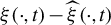 and
$b_\beta (\cdot ,t)-\widehat {b}_{\beta _{\mathsf {init}}}(\cdot ,t)$
 onto the dictionary
$\bar {{\mathsf {z}}}_{k_x}(x)$
 with respect to the weight g (see Section S8.1 of the Supplementary Material). This yields the oracle second-order estimating equation
$\widetilde {\psi }_{t,k}^{(2)}(\beta ) := \widehat {\psi }_t^{(1)}(\beta ) - \widetilde {\mathrm {B}}_{\psi ,t,k}(\beta )$
 , where

with
$\widetilde {\Omega }_{k_x} := {\mathbb {E}} \{K_{t,h}(T) \bar {{\mathsf {z}}}_{k_{x}} (X)\bar {{\mathsf {z}}}_{k_{x}}(X)^{\top }\} = \int _{{\mathcal {X}}} g(x)\bar {{\mathsf {z}}}_{k_{x}} (x)\bar {{\mathsf {z}}}_{k_{x}}(x)^{\top } {\mathrm d} x $
 treated as known. Here,
$\beta _{\mathsf {init}}$
 is an initial estimator of
$\beta ^{\ast }_t$
 computed from the nuisance sample. The oracle second-order estimator
$\widetilde {\beta }^{(2)}_{t}$
 is defined by solving
$\widetilde {\psi }_{t,k}^{(2)} (\beta )= 0$
 .
4.2 Convergence Rates of Higher-Order Estimators
To proceed, we impose a set of regularity conditions that closely parallel those for the finite-dimensional case. For brevity, we assume that Assumptions 3 and 6–8 hold with appropriate notational adjustments. Assumptions 4 and 5 are restated below in simplified form.
Assumption 14. For any
$t\in {\mathcal {T}}$
 : (i) the parameter space
${\mathcal {B}}$
 is compact and
$\beta ^{*}_t$
 is in the interior of
${\mathcal {B}}$
 ; (ii)
$\beta ^{\ast }_{t}$
 is the unique solution to
$\psi _{t} (\beta )= 0$
 , and
$\inf _{|\beta - \beta ^{\ast }_{t}| \geq \epsilon } |\psi _{t} (\beta )|> 0$
 for every
$\epsilon> 0$
 ; and (iii)
$\psi _{t} (\beta )$
 is continuously differentiable in
$\beta $
 with
$\nabla _{\beta } \psi _{t} (\beta ^{\ast }_{t})> 0$
 .
Additionally, we impose the following smoothness conditions on the nuisance functions and their estimators, which facilitate kernel smoothing and are standard in nonparametric estimation.
Assumption 15. The functions
$t \mapsto \xi (x, t)$
 and
$t \mapsto \mathsf {p}_{T}(t)$
 ,
$t \mapsto \widehat {\xi }(x, t)$
 are
$\alpha _{1}$
 -times continuously differentiable with uniformly bounded derivatives for any
$x \in {\mathcal {X}}$
 . Analogously,
$t \mapsto b_{\beta } (x, t)$
 and
$ t \mapsto \widehat {b}_{\beta } (x, t)$
 are
$\alpha _{2}$
 -times continuously differentiable with uniformly bounded derivatives for any
$x \in {\mathcal {X}}$
 and
$\beta \in {\mathcal {B}}$
 .
Theorem 6 is the main result of this section, characterizing the convergence rate of
$\widetilde {\beta }^{(2)}_t$
 . To reduce clutter, define
$\Delta _{b,t} (X;\beta ) := b_{\beta } (X,t) - \widehat {b}_{\beta _{\mathsf {init}}} (X,t)$
 and
$\Delta _{\xi ,t} (X) := \xi (X,t) - \widehat {\xi } (X,t).$

Theorem 6. Suppose that Assumptions 3, 6–8, and 13–15 hold. Let
$\widetilde {r}_{n,\mathsf {np}} \to 0$
 be a diminishing sequence as
$n\to \infty $
 . Suppose that
$ h (\log n)^2 \to 0 $
 ,
$(\widetilde {r}_{n,\mathsf {np}})^{\alpha _{0}} \log n \to 0$
 and

Then,
$\widetilde {\beta }^{(2)}_{t}$
 is a consistent estimator of
$\beta ^{*}_{t}$
 and satisfies

Here,
$\Pi ^{\perp }_{g} (f \mid \bar {{\mathsf {z}}}_{k_x}) (\cdot ) := f (\cdot ) - \int _{{\mathcal {X}}} f(x) \bar {{\mathsf {z}}}_{k_x} (x)^{\top } g(x) {\mathrm d} x \widetilde {\Omega }_{k_x}^{-1} \bar {{\mathsf {z}}}_{k_x} (\cdot )$
 denotes the orthocomplement of the g-weighted projection onto
$\bar {{\mathsf {z}}}_{k_x}$
 , and
$\|f\|_{g,2}^{2} = \int _{{\mathcal {X}}} f(x)^2g(x){\mathrm d} x$
 .
The proof of Theorem 6 is given in Section S8.1 of the Supplementary Material and closely follows that of Theorem 2. Using a similar decomposition, we first establish consistency by showing
${\mathbb {E}} (|\widetilde {\beta }^{(2)}_t - \beta ^*_t|) \lesssim \widetilde {r}_{n,\mathsf {np}} \to 0$
 . Building on this preliminary rate, we refine the analysis to the local region
$\{\beta \in {\mathcal {B}}: |\beta - \beta _{t}^{\ast }| \lesssim \widetilde {r}_{n,\mathsf {np}} \}$
 to obtain the final convergence rate. The key difference lies in the kernel-weighted U-processes introduced by the kernel function. To apply the maximal inequality from Section S6.2 of the Supplementary Material, each term in the Hoeffding decomposition must be carefully controlled with bandwidth-dependent envelopes, requiring a refined and delicate argument. These technical calculations distinguish our analysis from that of Kennedy et al. (Reference Kennedy, Ma, McHugh and Small2017), where the target parameter is explicitly defined and does not require such U-process techniques.
Remark 11. Following the same argument in Remark 7, we have

where
$\beta ^\dagger $
 lies between
$\beta _{\mathsf {init}}$
 and
$\beta ^{\ast }_{t}$
 . Assume that
$\Delta _{\xi ,t}(\cdot )$
 is
$s_{1}$
 -Hölder smooth, while
$\Delta _{b,t} (\cdot ;\beta _{\mathsf {init}})$
 and
$\nabla _{\beta }b_{\beta ^{\dagger }} (\cdot ,t)$
 are
$s_2$
 -Hölder smooth. With an appropriate basis
$\bar {{\mathsf {z}}}_{k_{x}}$
 , we have

Thus, if
$|\beta _{\mathsf {init}} - \beta ^{*}_t| = O_{\mathbb {P}}(1)$
 , Theorem 6 gives

Choosing
$k_x \asymp nh$
 makes the variance of order
$(nh)^{-1/2}$
 , reducing the rate to
$(nh)^{-(s_1+s_2)/d} + (nh)^{-1/2} + h^{\alpha _1 \wedge \alpha _2}$
 . If the average smoothness satisfies
$(s_1+s_2)/(2d) \geq 1/4$
 and
$h \asymp n^{-1/(2(\alpha _1 \wedge \alpha _2)+1)}$
 , we obtain the rate
$n^{-(\alpha _1 \wedge \alpha _2)/(2(\alpha _1 \wedge \alpha _2)+1)}$
 .
Remark 12. Our HOE
$\widetilde {\beta }_t^{(2)}$
 is related to two existing proposals for ADRF estimation. First, Colangelo and Lee (Reference Colangelo and Lee2026) develop a kernel-based DML estimator motivated by an approximate first-order influence function obtained through kernel localization around a target treatment value. Their estimator takes the form

where
$\widehat {\mu }(x,t) := {\mathbb {E}} [Y \mid X=x, T=t]$
 . They establish asymptotic normality of
$\widehat {\beta }_{\mathrm {CL}}$
 under high-level regularity conditions, including the key product-rate requirement
$\sqrt {n h}\|\widehat {\mathsf {p}}_{T \mid X} (T = t \mid \cdot )-\mathsf {p}_{T \mid X} (T = t \mid \cdot )\|_{\mathbb {P},2} \cdot \|\widehat {\mu }(\cdot ,t) - \widehat {\mu }(\cdot ,t)\|_{\mathbb {P},2}\to 0$
 . Second, Bonvini and Kennedy (Reference Bonvini and Kennedy2022) propose a second-order estimator (the BK estimator) based on the truncated parameter approach of HOIFs (Robins et al., Reference Robins, Li, Tchetgen Tchetgen and van der Vaart2008):

In essence,
$\widetilde {\beta }_{\mathrm {BK}}$
 can be viewed as a higher-order extension of
$\widehat {\beta }_{\mathrm {CL}}$
 for ADRF.
Our oracle second-order estimator is obtained by solving

Notably, because
$b_\beta (X,t) - \widehat {b}_{\beta _{\mathsf {init}}}(X,t) = \mu (X,t) - \beta - \widehat {\mu }(X,t) + \beta _{\mathsf {init}}$
 and
$\Pi _g^{\perp }[\beta - \beta _{\mathsf {init}} \mid \bar {{\mathsf {z}}}_{k_x}] \equiv 0$
 for any
$\beta $
 , the convergence rate in Theorem 6 simplifies to

This rate coincides with that of Theorem 1 in Bonvini and Kennedy (Reference Bonvini and Kennedy2022), confirming that our framework generalizes their result to a broader class of nonparametric GTM parameters, including the QDRF (Example 8) as a special case.
Remark 13. When the unknown matrix
$\widetilde {\Omega }_{k_x}$
 in
$\widetilde {\psi }_{t,k}^{(2)}$
 is replaced by an estimator
$\widehat {\Omega }_{k_x}$
 computed from the nuisance sample, we obtain the feasible estimator
$\widehat {\psi }_{t,k}^{(2)}$
 . Correspondingly, we define the feasible estimator
$\widehat {\beta }_t^{(2)}$
 for
$\beta _t^*$
 as the solution to
$\widehat {\psi }_{t,k}^{(2)}(\beta ) = 0$
 . Following similar arguments as in Theorem 3, the convergence rate of
$\widehat {\beta }_t^{(2)}$
 satisfies

This bound mirrors the structure established in Theorem 4 for the finite-dimensional case and can serve as a building block for establishing asymptotic normality of the feasible estimator under appropriate conditions on
$\widehat {\Omega }_{k_x}$
 .
5 NUMERICAL EXPERIMENTS
5.1 Simulation Studies
In this section, we conduct a proof-of-concept simulation study comparing the performance of our proposed HOE with two competing methods that do not utilize the HOIF framework. We focus on estimating the QTE parameter with binary treatment,
$\boldsymbol {\beta }^* = (\beta _{0}^*, \beta _{1}^*)^{\top }$
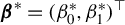 , as described in Example 2. Recall that
$\beta _{1}^*$
 (resp.
$\beta _{0}^*$
 ) denotes the
$\tau $
 -quantile of the treatment (resp. control) group. We choose
$\tau = 25\%$
 in this simulation. Following Xu et al. (Reference Xu, Liu and Liu2022) and Liu et al. (Reference Liu, Mukherjee, Newey and Robins2017), we simulate data from the following two data-generating mechanisms with different numbers of baseline covariates (
$d = 1$
 for Case 1 and
$d = 4$
 for Case 2):
-
• Case 1:
$$ \begin{align*} \left\{ \begin{array}{l} X \sim \mathrm{Uniform} ([-1, 1]), \\ T \mid X \sim \mathrm{Bernoulli} (\mathrm{expit} (\eta (0.5 \cdot X;s))), \\ Y (t) \mid X = (1 + 0.3 \cdot \eta (0.5 \cdot X;s)) \cdot t + 0.2 \cdot \varepsilon. \end{array} \right. \end{align*} $$
-
• Case 2:
$$ \begin{align*} \left\{ \begin{array}{l} X = (X_1,\ldots,X_4)^{\top} \sim \mathrm{Uniform} ([-1, 1]^4), \\ T \mid X \sim \mathrm{Bernoulli} (\mathrm{expit} (\eta (0.5 \cdot X_1;s))), \\ Y (t) \mid X = (1 + 0.3 \cdot \eta (0.5 \cdot X_1;s)) \cdot t + 0.2 \cdot \varepsilon, \end{array} \right. \end{align*} $$


where
$\varepsilon \sim N (0, 1)$
 ,
$\mathrm {expit} (x) = 1 / (1 + \exp (-x))$
 ,
$\eta (x; s) = \sum _{j \in J, l \in {\mathbb {Z}}} 2 ^{-j (s + 0.25)} w_{j, l}(x)$
 with
$J = \{0, 3, 6, 9, 10, 16\},$
 and
$w_{j,l}(\cdot )$
 is the D6 father wavelet functions. By construction,
$\eta (\cdot; s)$
 lies close to the boundary of Hölder-smooth functions with smoothness index s. We note that this is only an approximation, as exact infinite basis expansions are infeasible in simulations. Cases 1 and 2 share the same true outcome regression and propensity score. The only difference is that Case 2 includes three extra non-contributing covariates. In the analysis, we do not assume such knowledge so the basis
$\bar {{\mathsf {z}}}_{k}$
 depends on all four covariates by stacking the univariate spline basis blocks together with an intercept term
$\bar {{\mathsf {z}}}_{k} (x) = (1,\bar {{\mathsf {z}}}_{k_{1}} (x_{1})^{\top }, \bar {{\mathsf {z}}}_{k_{2}} (x_{2})^{\top }, \bar {{\mathsf {z}}}_{k_{3}} (x_{3})^{\top }, \bar {{\mathsf {z}}}_{k_{4}} (x_{4})^{\top })^{\top }$
 , which yields a basis vector of dimension
$k = \sum _{j = 1}^{4} k_{j}+1$
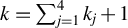 .
We vary
$s \in \{0.25, 0.4, 0.6\}$
 to examine its impact on estimator performance and to validate the theoretical results derived earlier. For each combination of sample size n and smoothness level s, we run 1,000 replications. In each replication,
$2n$
 observations are drawn and split equally into a nuisance sample and an estimation sample. We estimate
$\boldsymbol {\beta }^*$
 using three methods:
-
HOE: Our HOE is defined in Section 3.2. For each continuous covariate, we use a degree-1 B-spline expansion with the number of interior knots set to $\lceil n/100\rceil $
. As mentioned, we construct the basis
$\bar {{\mathsf {z}}}_k(x)$
by stacking the univariate spline basis blocks for all continuous covariates, together with an intercept term. Specifically, in Case 2,
$\bar {{\mathsf {z}}}_k(x) = (1, \bar {{\mathsf {z}}}_{k_1}(x_1)^\top , \bar {{\mathsf {z}}}_{k_2}(x_2)^\top , \bar {{\mathsf {z}}}_{k_3}(x_3)^\top , \bar {{\mathsf {z}}}_{k_4}(x_4)^\top )^\top ,$
with
$k_j=\lceil n/100\rceil +1$
and total dimension
$k=\sum _{j=1}^4 k_j + 1$
. On the nuisance sample, we estimate the stabilized weight function
$\widehat \xi $
via logistic regression, obtain the initial estimator
$\boldsymbol {\beta }_{\mathrm {init}}$
by stabilized weighting using
$\widehat \xi $
, and estimate
$\widehat b_{\boldsymbol {\beta }_{\mathrm {init}}}$
also via logistic regression. -
GOE: The generalized optimization estimator of Ai et al. (Reference Ai, Linton, Motegi and Zhang2021), applied to both the nuisance and estimation samples. See Section S9.1 of the Supplementary Material for its explicit form.
-
LDML: The LDML estimator of Kallus et al. (Reference Kallus, Mao and Uehara2024), implemented with the same settings as in Section 6.1 of that paper, where all nuisance functions are estimated via logistic regression.




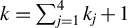


Both Figure 3 (for Case 1) and Figure 4 (for Case 2), displaying simulation results for the QTE
$\beta _1^\ast - \beta _0^\ast $
 , show that when the smoothness parameter s is low (e.g.,
$s = 0.25$
 or more precisely s is close to
$0.25$
 ), our HOE substantially outperforms both GOE and LDML, achieving lower MSE and absolute bias, especially when the sample size n is relatively large. In particular, the HOE is empirically
$\sqrt {n}$
 -consistent even when s is near 0.25 (the lower right panels of Figures 3 and 4). This advantage stems from the difficulty of estimating nuisance functions under low smoothness, which induces large first-stage bias—due to errors in both the nuisance parameter estimates and the initial estimator
$\boldsymbol {\beta }_{\mathsf {init}}$
 . Consequently, GOE and LDML fail to achieve
$\sqrt {n}$
 -consistency (see the lower-right panel). As s increases, all three methods exhibit improvements, with bias, variance, and MSE all decreasing. These empirical findings are consistent with our theoretical results, which indicate that the HOE enjoys improved statistical properties when the Hölder smoothness of the nuisance parameters is low.
Results for the simulation study Case 1 of estimating the QTE,
$\beta _1^*-\beta _0^*$
 , where
$\beta _{1}^*$
 (resp.
$\beta _{0}^*$
 ) denotes the
$25\%$
 -quantile of the treatment (resp. control) group, using different methods, based on 1,000 Monte Carlo replications.
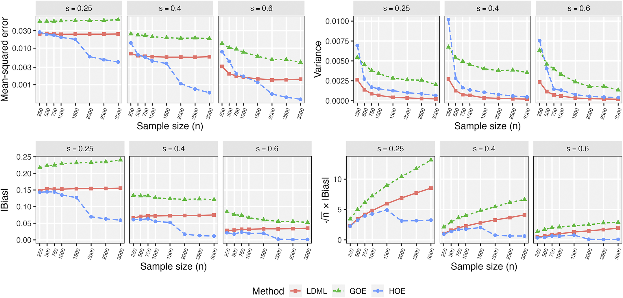
Figure 3 Long description
The image consists of four main sections, each containing three sub-panels corresponding to s = 0.25, s = 0.4, and s = 0.6. All graphs use Sample size (n) on the x-axis, ranging from 250 to 3000.
* Top-Left Section (Mean-squared error): The y-axis is on a log scale from 0.001 to 0.030. G O E (green triangles) remains highest and relatively flat. L D M L (red squares) is stable and lower than G O E. H O E (blue circles) starts near L D M L but decreases sharply as n increases, becoming the lowest error method at larger sample sizes.
* Top-Right Section (Variance): The y-axis ranges from 0.0000 to 0.0100. All three methods show an asymptotic decay toward zero as n increases. H O E starts with the highest variance at n = 250 but drops rapidly to converge with L D M L, while G O E maintains a higher variance throughout.
* Bottom-Left Section (Absolute Bias): The y-axis ranges from 0.00 to 0.25. G O E shows the highest bias, which slightly increases with n. L D M L shows a constant, moderate bias. H O E shows a bias that decreases significantly as n increases, especially after n = 1500.
* Bottom-Right Section (Square root of n times Absolute Bias): The y-axis ranges from 0 to 10. G O E and L D M L show linear increases, indicating bias does not vanish faster than the square root of n. H O E shows a non-linear trend that stabilizes or decreases at higher n values, particularly for s = 0.4 and s = 0.6.
A legend at the bottom identifies the methods: L D M L (red line with squares), G O E (green dashed line with triangles), and H O E (blue dashed line with circles).
Results for the simulation study Case 2 of estimating QTE,
$\beta _1^*-\beta _0^*$
 , where
$\beta _{1}^*$
 (resp.
$\beta _{0}^*$
 ) denotes the
$25\%$
 -quantile of the treatment (resp. control) group, using different methods, based on 1,000 Monte Carlo replications.
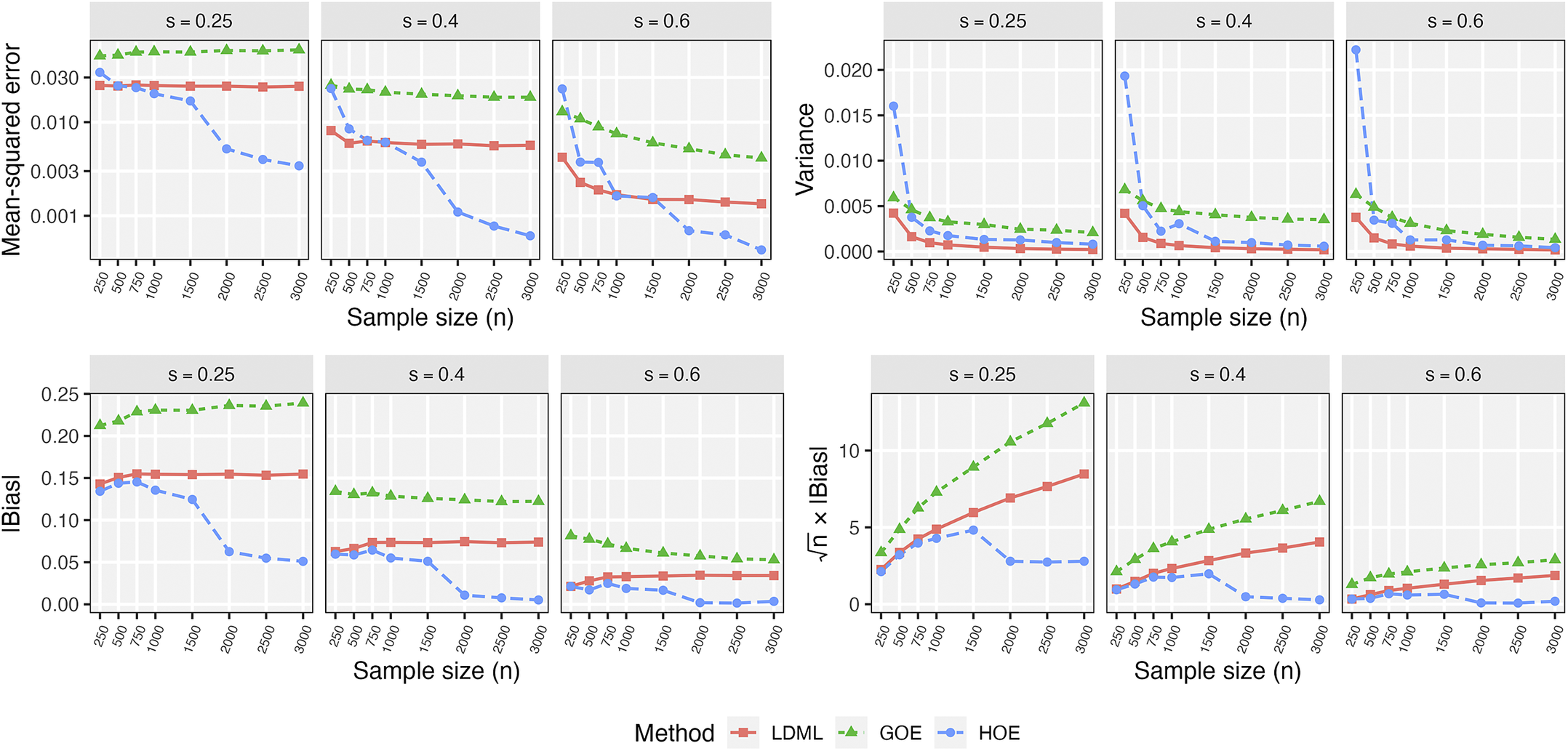
Figure 4 Long description
The grid consists of four main rows or sections, each containing three panels corresponding to s equals 0.25, 0.4, and 0.6. The x-axis for all graphs is Sample size n, ranging from 250 to 3000. A legend at the bottom identifies three methods: L D M L (red line with squares), G O E (green dashed line with triangles), and H O E (blue dashed line with circles).
* Top-left section (Mean-squared error): The y-axis uses a logarithmic scale from 0.001 to 0.030. G O E remains highest and relatively flat. L D M L shows a slight downward trend. H O E starts high but drops sharply as n increases, especially for s equals 0.4 and 0.6.
* Top-right section (Variance): The y-axis ranges from 0.000 to 0.020. All methods show an asymptotic decrease toward zero as sample size increases. H O E starts with the highest variance at n equals 250 but converges quickly.
* Bottom-left section (Absolute Bias): The y-axis ranges from 0.00 to 0.25. G O E maintains the highest bias across all s values. L D M L is stable and lower than G O E. H O E shows a significant decrease in bias as n increases, eventually becoming the lowest for larger sample sizes.
* Bottom-right section (Square root of n times Absolute Bias): The y-axis ranges from 0 to 10. G O E and L D M L show linear increases as n grows. H O E shows an initial increase followed by a plateau or decrease, indicating better convergence properties.
Figures 5 and 6 (for Case 1) and Figures 7 and 8 (for Case 2) in the Supplementary Material present normal QQ-plots of our HOEs for
$\beta _0^*$
 and
$\beta _1^*$
 across all
$(n,s)$
 combinations. These plots support the theoretical conclusion (Theorem 4) that the HOEs are asymptotically normal under appropriate scaling.
Finally, we perform sensitivity analyses to examine whether our HOE is sensitive to the choice of k or to the initial estimator
$\boldsymbol {\beta }_{\mathsf {init}}$
 . Recall that, for each continuous covariate, we use a degree-1 B-spline basis with
$\lceil n/100\rceil $
 interior knots. To examine the sensitivity to the choice of k, we multiply
$ n/100$
 by a factor
$\lambda \in \{0.75,1,1.25\}$
 , so that the number of knots varies over
$\lceil \lambda n/100\rceil $
 , resulting in
$k = d\cdot (\lceil \lambda n/100\rceil + 1) + 1$
 . Figure 9 in the Supplementary Material reports the empirical bias, variance, and mean squared error for HOE QTE estimator across different values of
$\lambda $
 for both Cases 1 and 2 with
$n=2,000$
 and
$s=0.25$
 , based on 1,000 Monte Carlo replications. The figure shows the expected bias–variance tradeoff: as k increases, the empirical bias of the HOE decreases, whereas the empirical variance increases. In practice, one may choose k such that the point estimates do not differ as much compared to the increase in variance. Here, for both Cases 1 and 2,
$\lceil n / 100 \rceil $
 is a reasonable choice. A more thorough study of how to choose k is left to a future work that is dedicated to the problem of constructing data-driven basis.
To assess sensitivity to the initial estimator
$\boldsymbol {\beta }_{\mathsf {init}}$
 , we perturb it deterministically as
$ \boldsymbol {\beta }_{\mathsf {init}}^{(\delta )} = \boldsymbol {\beta }_{\mathsf {init}} + \delta \cdot (-1,1)^\top , $
 with
$ \delta \in \{-0.5,-0.25,0,0.25,0.5\}$
 . Here, the perturbation level
$\delta $
 controls both the magnitude and the direction of the perturbation. Figure 10 in the Supplementary Material reports boxplots of the estimation error of the HOE QTE estimator across different values of
$\delta $
 for both Cases 1 and 2, in the setting
$n=2,000$
 and
$s=0.25$
 , based on 1,000 Monte Carlo replications. The results reported in Figure 10 in the Supplementary Material suggest that HOE is fairly robust to moderate perturbations in the initial estimator. However, when the perturbation becomes too large, the estimator becomes less stable, as reflected by the increased dispersion and a slightly greater number of outliers.
5.2 Real Data Analysis
In this section, we apply our HOEs to estimate the QTE of 401(k) plan eligibility on household wealth, using the Survey of Income and Program Participation (SIPP) data studied in Abadie (Reference Abadie2003), Benjamin (Reference Benjamin2003), Chernozhukov and Hansen (Reference Chernozhukov and Hansen2004), and Kallus et al. (Reference Kallus, Mao and Uehara2024). The sample contains 9,915 observations. The treatment T indicates eligibility for a 401(k) plan, and the outcome Y is net financial assets; our goal is to assess whether 401(k) eligibility increases household saving. The dataset consists of a set of pre-treatment covariates X, including age, income, family size, education, marital status, two-earner status, DB pension status, IRA participation, and homeownership (see Chernozhukov and Hansen, Reference Chernozhukov and Hansen2004, Sect. 3, for details). Recently, Kallus et al. (Reference Kallus, Mao and Uehara2024) analyzed this dataset using LDML estimators. We implement our higher-order debiased estimators on the same dataset to provide a proof of concept for their application in real-world settings.
As in our simulation studies, we split the sample into two folds. With the nuisance sample, we compute the initial estimator
$\widehat {\boldsymbol {\beta }}_{\mathsf {init}}$
 by stabilized weighting and estimate both the stabilized weights
$\widehat \xi $
 and the generalized outcome regression model
$\widehat {b}_{\boldsymbol {\beta }_{\mathsf {init}}}$
 using four learners: random forest, boosting, LASSO, and a one-hidden-layer neural network. Random forests are implemented using the R package randomForest, boosting using gbm, LASSO using hdm, and the one-hidden-layer neural network using nnet. For LASSO, we include polynomial terms of degree 6 for age, 8 for income, 4 for education, and 2 for family size, together with all binary covariates, and all pairwise interactions among these terms, resulting in a total of 275 predictors.
In the debiasing step, we use degree-2 B-spline expansions for the continuous covariates income, age, family size, and education, with interior knot numbers
$(\lceil n/200\rceil ,\lceil n/200\rceil ,4,2)=(25,25,4,2)$
 , respectively. We then construct
$\bar {{\mathsf {z}}}_k(x)$
 by stacking the resulting univariate spline basis blocks with the binary covariates and an intercept term. This choice accounts for the heterogeneous supports of the continuous covariates: income and age vary over wide ranges, while family size and education take values on smaller grids. It also ensures numerical stability of
$\widehat {\Sigma }_k$
 by avoiding very small eigenvalues. For comparison, we also report LDML estimates under the same settings as Section 6.2 of Kallus et al. (Reference Kallus, Mao and Uehara2024) (with
$K=5$
 ), using a fixed two-fold split without re-randomizing folds to maintain transparency.
Table 2 reports the point estimates of 25%, 50%, and 75% QTEs. Overall, QTE estimates are generally stable among different nuisance learners, suggesting that the bias of the LDML estimator may be relatively small in this application. The higher-order estimates are close to their LDML counterparts, further strengthening this conclusion. Consequently, the difference between the HOE and the LDML estimator provides empirical evidence on the magnitude of the potential bias of the LDML estimator (Liu et al., Reference Liu, Mukherjee and Robins2024).
The QTE of 401(k) eligibility in thousand dollars estimated by LDML and higher-order estimates (HOEs) using different regression methods (LASSO, neural network, boosting, and random forests).
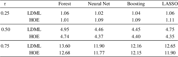
Table 2 Long description
The table is organized by quantile levels (tau) of 0.25, 0.50, and 0.75. For each level, two estimation types are provided: L D M L and H O E.
* At tau equals 0.25:
- L D M L: Forest 1.06, Neural Net 1.02, Boosting 1.04, LASSO 1.06.
- H O E: Forest 1.01, Neural Net 1.09, Boosting 1.09, LASSO 1.11.
* At tau equals 0.50:
- L D M L: Forest 4.95, Neural Net 4.46, Boosting 4.45, LASSO 4.75.
- H O E: Forest 4.74, Neural Net 4.37, Boosting 4.40, LASSO 4.35.
* At tau equals 0.75:
- L D M L: Forest 13.60, Neural Net 11.90, Boosting 12.16, LASSO 12.65.
- H O E: Forest 12.68, Neural Net 11.77, Boosting 12.15, LASSO 11.90.
All values represent thousand dollars.
Note: Here,
$\tau \in \{25\%,50\%,75\%\}$
 denotes the quantile level of QTE.
We examine sensitivity to both the choice of k and the initial estimator
$\boldsymbol {\beta }_{\mathsf {init}}$
 . To assess sensitivity to k, we increase the number of interior knots for age by multiplying
$n/200$
 by a factor
$\lambda \in \{0.75,1,1.25\}$
 while keeping other knot numbers fixed. The HOEs perform reasonably well in this range, as shown in Table 3 in the Supplementary Material. Stability is ensured by the numerical inversion of
$\widehat {\Sigma }_k$
 when k is relatively small compared to n, whereas the performance degrades if
$\widehat {\Sigma }_k$
 approaches singularity. Therefore, a heuristic strategy to explore in the future is to increase k (via knots or degree) until numerical instability occurs. Developing such data-driven rules for selecting k and constructing
$\bar {{\mathsf {z}}}_k$
 remains an important direction.
Sensitivity to
$\boldsymbol {\beta }_{\mathsf {init}}$
 is examined similarly to the simulation studies. We find that the HOE is generally robust to small perturbations of
$\widehat {\boldsymbol {\beta }}_{\mathsf {init}}$
 , as shown in Table 4 in the Supplementary Material.
6 CONCLUDING REMARKS
In this article, we have constructed HOEs for implicitly defined parameters frequently encountered in econometrics, including ATEs and QTEs as special cases. By applying the HOIFs framework to implicitly defined parameters, we have contributed to the existing econometrics and causal inference literature. Our proposed estimators achieve improved convergence rates compared to first-order methods, which requires only that the initial estimator be consistent rather than imposing stringent rate conditions. For binary-treatment QTE, our estimator attains
$\sqrt {n}$
 -consistency under the Hölder smoothness condition
$s/d> 1/4$
 , substantially relaxing the requirements of existing approaches and matching the minimal Hölder smoothness condition for the ATE to be
$\sqrt {n}$
 -estimable. We have also extended the framework to infinite-dimensional GTMs, providing a unified approach for estimating nonparametric causal functions such as dose–response curves.
Several directions remain for future research. First, while we focused on second-order estimators assuming that
$\Sigma _k$
 can be estimated sufficiently accurately, relaxing this assumption would require further advances in the theory of higher-order U-processes. Second, extending our framework to other complexity-reducing assumptions, such as sparsity classes (Athey, Imbens, and Wager, Reference Athey, Imbens and Wager2018), remains an open question. Third, with slight modifications, our framework is also expected to be able to address endogeneity problems (including nonparametric and many weak IV models) (Breunig and Chen, Reference Breunig and Chen2024). Finally, it would be interesting to compare our higher-order debiased estimator with other related bias-correction or bias-aware methods (Armstrong, Kolesár, and Kwon, Reference Armstrong, Kolesár and Kwon2020; Zheng, Bonvini, and Guo, Reference Zheng, Bonvini and Guo2025; Bonhomme et al., Reference Bonhomme, Jochmans, Newey and Weidner2026).
SUPPLEMENTARY MATERIAL
The supplementary material for this article can be found at https://doi.org/10.1017/S0266466626100516.
FUNDING STATEMENT
The research related to this article is supported by funds from the National Key R&D Program of China [Grant No. 2022YFA1008300] (Zheng Zhang), NSFC [Grant No. 12471274] (Lin Liu), the Fundamental Research Funds for the Central Universities and the Research Funds of Renmin University of China [Project No. 23XNA025] (Zheng Zhang), and the Science and Technology Talent and Platform Program of Yunnan Province [Grant No. 202605AF350070] (Lin Liu).
COMPETING INTERESTS
The authors declare that no competing interests exist.