Effectiveness of environmental decontamination as an infection control measure

M. BANI-YAGHOUB; R. GAUTAM; D. DÖPFER; C. W. KASPAR; R. IVANEK

doi:10.1017/S0950268811000604

Effectiveness of environmental decontamination as an infection control measure

Published online by Cambridge University Press: 18 May 2011

C. W. KASPAR and

M. BANI-YAGHOUB*: Affiliation:
Department of Veterinary Integrative Biosciences, College of Veterinary Medicine and Biomedical Sciences Texas A & M University, College Station, TX, USA
R. GAUTAM: Affiliation:
Department of Veterinary Integrative Biosciences, College of Veterinary Medicine and Biomedical Sciences Texas A & M University, College Station, TX, USA
D. DÖPFER: Affiliation:
Department of Medical Sciences, School of Veterinary Medicine, University of Wisconsin, Madison, WI, USA
C. W. KASPAR: Affiliation:
Department of Bacteriology, University of Wisconsin, Madison, WI, USA
R. IVANEK: Affiliation:
Department of Veterinary Integrative Biosciences, College of Veterinary Medicine and Biomedical Sciences Texas A & M University, College Station, TX, USA
*: *Author for correspondence: Dr M. Bani-Yaghoub, Texas A & M University, Veterinary Integrative Biosciences, 4458 TAMUS College Station, TX 77843-4458, USA. (Email: MBani@cvm.tamu.edu)

Article contents

Summary
INTRODUCTION
THE MODEL
EQUILIBRIUM AND ECOLOGICAL STABILITY
DISEASE CONTROL AND MANAGEMENT
DISCUSSION
References

Rights & Permissions

Summary

The effectiveness of environmental decontamination (ED) as a measure in the control of infectious diseases is controversial. This work quantifies the effectiveness of ED by analysing the transmission of pathogens from the environment to susceptible hosts in a Susceptible–Infected–Susceptible model. Analysis of the model shows that ED can render a population disease-free only when the duration of infection (D) is within a certain range. As host-to-host transmission rate is increased, D falls outside this range and the higher levels of ED have a diminishing return in reducing the number of infected hosts at endemic equilibrium. To avoid this, ED can be combined with other control measures, such as treating infected individuals to push the duration of infection into the specified range. We propose decision criteria and minimum ED efforts required for control policies to be effective.

Keywords

Decision criteria decontamination infection control pathogen persistence SISp model

Information

Type: Original Papers
Information: Epidemiology & Infection , Volume 140 , Issue 3 , March 2012, pp. 542 - 553
DOI: https://doi.org/10.1017/S0950268811000604 [Opens in a new window]
Copyright: Copyright © Cambridge University Press 2011

INTRODUCTION

The inanimate environment contributes to the transmission of infectious diseases. Specifically, contaminated food, water, soil, objects and contact surfaces have been associated with disease transmission [Reference Boone and Gerba1–Reference Scott and Bloomfield4]. A contaminated environment is recognized by regulatory and health organizations as an exposure source [Reference Manangan3, 5, 6] and the inanimate environment can serve as a reservoir of infectious disease to humans and animals [Reference Scott and Bloomfield4, Reference Boyce7]. Moreover, free-living pathogens can be transmitted from the environment to susceptible hosts [Reference Caraco and Wang8–Reference Evans, Entwistle, Fuxa and Tanada11] and therefore effective environmental decontamination (ED) serves as an infection control measure.

The present work is concerned with the effects of ED on disease transmission in a host population. Here, decontamination is defined as a reduction of the pathogen load in the environment by any method (e.g. cleaning and disinfecting) other than natural decay. The main question is whether ED can be an effective control measure. A clear answer to this question requires a deeper understanding of the underlying mechanisms governing pathogen–host–environment interactions. However, the role of ED as an infection control measure is controversial. Several studies report the benefits of cleaning and disinfecting in the control of infectious disease [Reference Cozad and Jones12–Reference Rutala and Wenzel14]. Whereas other works suggest that decontamination of the inanimate environment is only a minor factor [Reference Maki15, Reference Daschner and Schuster16]. There is a need to quantify the effectiveness of ED in the control and prevention of infections.

Pathogen transmission through the environment has been modelled in previous studies describing various infectious disease dynamics [Reference Anderson and May9, Reference Ayscue17–Reference Turner20]. Nevertheless, the effects of ED in the control and prevention of infection have been less studied through mathematical models of infectious disease. When an infection does not confer immunity, a Susceptible–Infected–Susceptible (SIS) model can be used to investigate the dynamics of host–pathogen interactions (see e.g. [Reference Brauer, van den Driessche and Jianhong21, Reference Allen22]). Here, the basic SIS model is extended by including transmission of a pathogen from the environment to susceptible hosts. Thus the extended SIS _p model is used to study the effectiveness of ED. The subscript ‘p’ indicates the free-living pathogen considered in the model.

The primary goal of the present work is to determine whether ED can prevent the establishment of infection within a host population. Specifically, by considering that a susceptible host can be infected by direct contact with an infected host and indirectly through the contaminated environment, analysis of the SIS _p model will determine whether interruptions in pathogen transmission occur as a result of ED. Moreover, the effectiveness of ED alone or combined with other control measures is quantified through a differential technique well-known in multivariable calculus.

The rest of this paper is organized as follows. The next section describes the model's assumptions and introduces the SIS _p model. Further sections are concerned with the basic reproduction number R ₀ and disease-free and endemic (E) equilibria; disease control strategies and the effectiveness of ED; and a final section delivers the main conclusions.

THE MODEL

The basic SIS model can be extended to various complicated models with age structure, delay and spatial dispersion. Nevertheless, complexity of the model could hinder interpretation of the model results. Therefore, we chose to study the effectiveness of ED in a simple scenario. In particular, for a spatially homogeneous population, we considered the following model assumptions:

(1) Total population size is constant over time. In addition, no births or deaths are considered.
(2) Infection does not confer immunity; individuals become susceptible again after they recover from the infection.
(3) A susceptible host may become infected after a direct adequate contact with an infected host.
(4) A susceptible host may become infected through contact with a sufficient number of free-living pathogens in the environment.
(5) Both host-to-host and environment-to-host transmission terms are ‘density-dependent’, i.e. it is assumed that the force of infection increases with increased host population size.

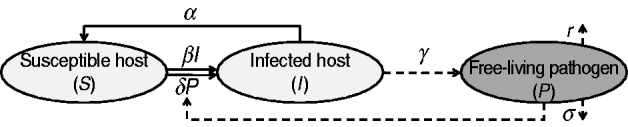
Infected individuals shed the pathogen over a given period of time. Although the shedding level may vary over time [Reference Ivanek23], a constant rate of shedding is assumed here. The presence of the pathogen in the environment is maintained by hosts' pathogen shedding while it is challenged by natural decay and pathogen removal strategies (i.e. decontamination). Figure 1 is a compartmental diagram for the proposed model and Table 1 summarizes the model elements. The system of ordinary differential equations representing the SIS _p model is given by

(1)

$\dot{S} \equals \minus \beta SI \plus \alpha I \minus \delta SP\comma \hfill$

(2)

$\dot{I} \equals \beta SI \minus \alpha I \plus \delta SP\comma \hfill$

(3)

$\dot{P} \equals \gamma I \minus \lpar r \plus \sigma \rpar P \minus \delta NP\comma \hfill$

where all constants α, β, …, are non-negative, the number of susceptible and infected individuals at time t [i.e. S(t) and I(t), respectively] are also non-negative. Since S(t)+I(t)=N for all t⩾0, S(t) can be replaced by N−I(t) and the system can be described by equations (2) and (3) alone. In contrast to the basic SIS model, the nonlinear model (1)–(3) cannot be solved by integration techniques. When δ=0 (i.e. the host does not become infected by contacting the contaminated environment), the system is decoupled. In this case equations (1) and (2) represent the basic SIS model with no births, deaths or immunity; equation (3) indicates the dynamics of the pathogen at a free-living stage.

Fig. 1.

A schematic representation of the SIS _p model. Solid and dashed lines indicate the dynamics of host and free-living pathogen, respectively.

Table 1.

Summary of the notations used in the model

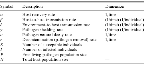
The relationship between r and the more intuitive representation of decontamination as the proportion of pathogens removed (P _removed) from the environment per unit time is defined with P _removed =(1− e^−r)×100.

In the ‘Dimension’ column, the term individual refers to the number of host or pathogen; both δP and βI have the dimension 1/time.

EQUILIBRIUM AND ECOLOGICAL STABILITY

Equilibrium analysis

The disease-free (DF) and E equilibria of the SIS _p model (1)–(3) are respectively given by

(4)

$\lpar S_{{\rm DF}} \comma I_{{\rm DF}} \comma P_{{\rm DF}} \rpar \equals \lpar N\comma 0\comma 0\rpar \comma \hfill$

and

(5)

$\lpar S_{\rm E} \comma I_{\rm E} \comma P_{\rm E} \rpar \equals \lpar S{ \ast } \comma N \minus S{ \ast } \comma P{ \ast } \rpar \comma \hfill$

where

(6)

$S{ \ast } \equals \alpha \lpar r \plus \sigma \plus \delta N\rpar \sol \lpar \delta \gamma \plus \beta \lpar r \plus \sigma \plus \delta N\rpar \rpar \comma\hfill$

(7)

$P{ \ast } \equals \gamma I{ \ast } \sol \lpar r \plus \sigma \plus \delta N\rpar.\hfill$

Since I*=N−S*>0, from equation (6) we get that the E equilibrium does not exists if

(8)

$N\lpar \beta \plus \delta \gamma \sol \lpar r \plus \sigma \plus \delta N\rpar \rpar \sol \alpha \lt 1.\hfill$

Note that the system (1)–(3), is subject to the constraint S(t)+I(t)=N for all t⩾0; hence (S, I, P)=(0, 0, 0) is not an equilibrium. The local and global stability analysis of DF and E equilibria are provided in Appendices A and B, respectively.

The basic reproduction number

The overall transmissibility fitness of an infectious agent in a host population is often quantified by the basic reproduction number R ₀, which is defined as the average number of secondary infections caused by a typical infected individual introduced into a totally susceptible population [Reference Anderson and May9, Reference Diekmann and Heesterbeek24]. We used the next-generation matrix approach [Reference Chowell, Brauer and Chowell25–Reference Diekmann, Heesterbeek and Roberts27] to obtain R ₀. Similarly to [Reference Tien and Earn28] and [Reference Chapagain29], we considered both P and I as disease compartments (see Appendix C for derivation of the next-generation matrix K). The largest non-negative eigenvalue of K is defined as R ₀ and is given by

(9)

$R_{\setnum{0}} \equals N\beta \sol \alpha \plus N\delta \gamma \sol \lpar r \plus \sigma \plus \delta N\rpar \alpha.\hfill$

When R ₀>1, there will be a disease outbreak, whereas R ₀<1 leads to a disease-free population. Concerning control and prevention of disease, the value of R ₀ should remain below the threshold value of 1. Expressing 1/α as D, which denotes the duration of infection, equation (9) is rewritten as

(10)

$R_{\setnum{0}} \equals R_{\setnum{0}_{d} } \plus R_{\setnum{0}_{{in}} } \comma\hfill$

where $R_{\setnum{0}_{d} } \equals ND\beta$ and $R_{\setnum{0}_{{in}} } \equals ND\delta \gamma \sol \lpar r \plus \sigma \plus \delta N\rpar$ .

Hence the R ₀ in equation (9) is the summation of two values related to direct and indirect transmissions. In particular, $R_{\setnum{0}_{d} }$ and $R_{\setnum{0}_{{in}} }$ respectively correspond to the number of secondary infections through host-to-host and environment-to-host transmission caused by an infected individual in a totally susceptible population.

DISEASE CONTROL AND MANAGEMENT

Reduction of infection

Control of an endemic infection does not necessarily mean elimination of the infection from the host population. Here, the underlying question is whether decontamination of the inanimate environment can reduce the infection from a host population. Let the number of susceptible and infected individuals at the E equilibrium be functions of removal rate r denoted by S*(r) and I*(r), respectively. In equation (6), by taking the derivative of S*(r) with respect to r, we have

(11)

${\rm d}S{ \ast } \lpar r\rpar \sol {\rm d}r \equals \alpha \delta \gamma \sol \lpar \delta \gamma \plus \beta \lpar r \plus \sigma \plus \delta N\rpar \rpar ^{\setnum{2}}.\hfill$

Since I*(r)=N−S*(r) and dS*(r)/dr>0, I*(r) is a decreasing function of r. Hence in an endemic state, a more aggressive decontamination of the environment (i.e. higher values of r) gives rise to a reduction in the number of infected hosts. However, dS*(r)/dr is a decreasing function of r and therefore S*(r) is a concave function of r (see the curves in Fig. 2). Thus, ED can be effective only to a certain limit and it has a diminishing return (i.e. for each unit increase in the value of r there will be progressively smaller gain in terms of I*(r) reduction). In particular, by allowing r→∞ the highest number of susceptible hosts at E equilibrium is S*(inf ty)=α/β. Then we are looking for r _max such that

(12)

$\alpha \sol \beta \minus S{ \ast } \lpar r_{\max } \rpar \lt 1\comma \hfill$

with α/β>1. Substituting the right-hand side of equation (6) into (12) and solving for r, we have

(13)

$r_{\max } \equals \lpar \alpha \minus \beta \rpar \delta \gamma \sol \beta ^{\setnum{2}} \minus \lpar \sigma \plus \delta N\rpar \comma \hfill$

provided that the right-hand side of equation (13) is positive. Otherwise, r _max is defined as zero. For the values of r>r _max, S*(r) is increased by <1. Hence, more aggressive decontamination policies corresponding to values of r⩾r _max are not effective and I*(r) is reduced at most by 1. In general, the parameter r _max defines a threshold value for effectiveness of ED in reducing the number of infected hosts during the endemic state.

Fig. 2.

Depending on the intensity of host-to-host transmission rate β, a more aggressive environmental decontamination may increase the number of susceptibles S* (and therefore decrease the number of infected host I*) at endemic equilibrium. The diminishing return of r on S* (and therefore I*) is replaced with a linear relationship as β→0.

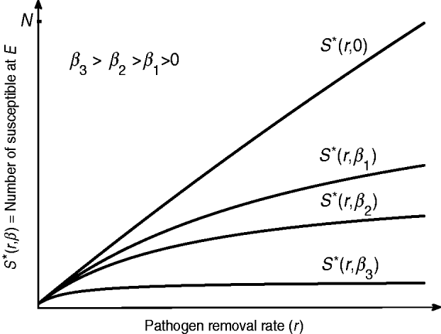
In terms of increasing S*, and therefore decreasing I*, the beneficial effect of ED is dependent on the host-to-host transmission rate β. From equation (13) we see that r _max increases for smaller values of β. Figure 2 indicates that the number of susceptible S* at E equilibrium is increased for smaller values of β. For diseases with a significant role of indirect transmission in the incidence of new cases, given that β≈0, the relationship between S* and r is almost linear. This includes nosocomial infections such as Clostridium difficile, vancomycin-resistant enterococci and methicillin-resistant Staphylococcus aureus for which there is a strong evidence of pathogen survival in environmental reservoirs [Reference Hota30].

Elimination of infection

From condition (8) it is concluded that the bifurcation parameter

(14)

$r_{\setnum{0}} \equals N\delta \gamma \sol \lpar \alpha \minus N\beta \rpar \minus \lpar \sigma \plus \delta N\rpar \comma \hfill$

exists only when

(15)

$N\beta \lt \alpha \lt N\beta \plus N\delta \gamma \sol \lpar \sigma \plus \delta N\rpar.\hfill$

Otherwise r ₀<0, which is biologically irrelevant. The parameter r ₀ defines the minimal decontamination effort required to eliminate the E equilibrium.

It can be shown that R ₀<1, only when condition (15) is satisfied and r>r ₀. Elimination of E equilibrium through ED is possible when it is applied in combination with other control measures such as treatments of infected individuals. In particular, if host recovery rate α is lower than the range specified in equation (15), an aggressive antibiotic treatment may decrease the duration of infection D and therefore it may push the recovery rate α into this range. In this case, any level of decontamination that provides r>r ₀ can return the population into the DF equilibrium. By dividing expression (15) by α, we get

(16)

$R_{\setnum{0}_{d} } \lt 1 \lt R_{\setnum{0}} \comma \hfill$

where R ₀ and $R_{\setnum{0}_{d} }$ are defined in equations (9) and (10). The condition (16) indicates that more aggressive decontamination can reduce the value of R ₀ to <1, only when the environmental factors are the main cause of infection (i.e. when $R_{\setnum{0}_{d} } \lt 1$ ). Conversely, $R_{\setnum{0}_{d} } {\ges} 1$ implies that R ₀>1 for any value of r. Therefore, no matter how aggressive ED is, a large host-to-host transmission rate β is sufficient for a disease outbreak.

Examples: Escherichia coli O157:H7 and typhoid fever

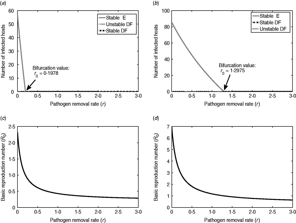
To illustrate and compare the effects of ED, we consider two scenarios of infection: E. coli O157:H7 in a dairy cattle herd and typhoid fever in a small community of people. Figure 3 represents the bifurcation diagrams and effects of ED (i.e. pathogen removal rate r) on I* and R ₀ for each of the cases. The parameter values associated with E. coli O157:H7 are based on previous studies. In particular, the host recovery rate α=0·048 was calculated as the reciprocal of the mean number of days for which a calf shed E. coli O157:H7 in faeces following initial infection [Reference Mechie, Chapman and Siddons31]. The host-to-host transmission rate and the environment-to-host transmission rate are assumed as β=10⁻⁴ and δ=3×10⁻¹³, respectively. The shedding rate γ=4×10⁸ for E. coli O157:H7 was estimated from the distribution of bacterial counts reported in Cray et al. [Reference Cray32]. The natural decay rate σ=0·118 of E. coli O157:H7 was obtained from [Reference Bolton33] using the initial count and the final count of bacteria at a given interval of time. Specifically, σ was estimated by σ=[log(C ₀)−log(C _t)]/Δt, where C ₀ is the initial count and C _t is the final count of bacteria and Δt is the interval of time between the measurement of the two counts. The parameter values related to typhoid fever were obtained from [Reference Gonzalez-Guzman19] under simplified assumptions, where the host's birth and death rates are zero and only the clinical stage of the infection is considered. By converting the rate of changes from years to days, the parameter values are N=100, α=0·0357, β=1·1992×10⁻⁴, δ=1·8396×10⁻⁵, γ=18·5822, σ=0·1425. Note that in both examples we have N=100; considering a higher value for N (or β) may result in $R_{{\setnum{0}}_d}$ >1, which will change the outcome prediction: ED cannot eradicate the infection and it may only reduce the number of infected hosts at the endemic state.

Fig. 3.

Illustration of the effectiveness of environmental decontamination for two infectious diseases. Plots on the left- and right-hand sides correspond respectively to Escherichia coli O157:H7 in cattle and typhoid fever in humans. (a, b) Bifurcation diagrams with respect to the parameter r. The minimal daily pathogen removal required for elimination of endemic equilibrium are 18% and 73%, respectively, which is obtained from $\lpar 1 \minus {\rm e}^{ \minus r_{\setnum{0}} } \rpar \times 100$ . (c, d) Plots of changes in R ₀ with respect to the decontamination level for E. coli O157:H7 and typhoid fever. The parameter values used to generate the diagrams are as follows. For E. coli O157:H7 and typhoid fever, respectively, N=100, 100; α=0·048, 0·0357; β=10⁻⁴, 1·1992×10⁻⁴; δ=3×10⁻¹³, 1·8396×10⁻⁵; γ=4×10⁸, 18·5822; σ=0·118, 0·1425; r ₀=0·1978 and r ₀=1·2975. DF, Disease free; E, endemic.

Impacts of parameter changes

The parameters of the SIS _p model (1)–(3) may change individually or simultaneously. In particular, a more aggressive ED corresponds to higher values of r; the shedding rate γ may increase due to presence of supershedders; the host-to-host transmission rate β may vary due to seasonal changes in contact behaviour. If the pathogens are not resistant to antibiotics, employing an antibiotic treatment will increase the host recovery rate α by reducing the duration of infection D and it may also decrease the shedding rate γ. Persistence of the free-living pathogen corresponds to the inverse of the natural decay rate σ. Then, σ may decrease when the pathogen adapts to the environment through some morphological and physiological changes [Reference Anderson and May34, Reference Bonhoeffer, Lenski and Ebert35].

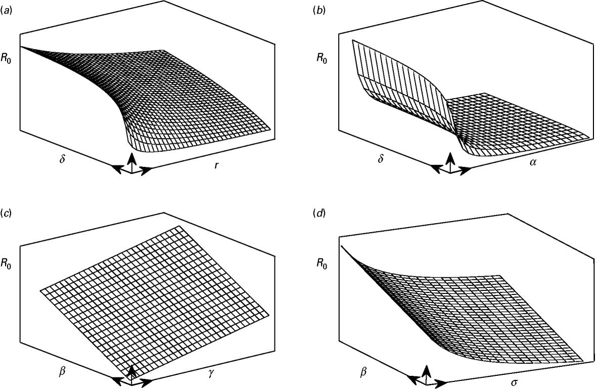
Concerning individual parameter changes, the impacts of parameter changes on $R_{\setnum{0}_{d} }$ , and $R_{\setnum{0}_{{in}} }$ and therefore R ₀, are discussed as follows. The value of $R_{\setnum{0}_{d} }$ increases with β linearly, while it parabolically decreases with α. In all other cases, $R_{\setnum{0}_{d} }$ remains unchanged. The value of $R_{\setnum{0}_{{in}} }$ decreases parabolically with α, r and σ, while it increases parabolically with δ. An increase in N results in a parabolic increase in $R_{\setnum{0}_{{in}} }$ , whereas it increases $R_{\setnum{0}_{d} }$ linearly. In terms of disease control and management, there is a sharp difference between the parabolic and the linear changes. When the value of δ (or r, σ) is close to zero any small change makes a huge difference in the value of $R_{\setnum{0}_{{in}} }$ and therefore R ₀. The changes of R ₀ with respect to α close to zero are even more pronounced since both $R_{\setnum{0}_{d} }$ and $R_{\setnum{0}_{{in}} }$ decrease parabolically with α. On the other hand these parameters have diminishing effect in terms of gain in infection control as they move away from zero. Hence, linear increases of R ₀ due to increases of β or γ can hardly be controlled by increases in α, r, σ (or decreases in δ) when these parameters are away from zero. Figure 4 is a conceptual illustration of the cases mentioned above.

Fig. 4.

A conceptual illustration of the parabolic and linear changes in the value of R ₀ as a result of parameter changes. (a) An increase of δ results in a parabolic increase in the value of R ₀, whereas increases in γ give rise to parabolic decreases in R ₀. (b) Comparison with the previous case, since α is present both in $R_{\setnum{0}_{d} }$ and $R_{\setnum{0}_{{in}} }$ , it has impacts stronger than γ in controlling the increases in R ₀. (c) The value of R ₀ is linearly increased with parameters β and γ. (d) Similar to r and α, the parameter σ has a diminishing return in controlling the linear increases in R ₀ due to increases in β or δ.

Control of pathogen trait changes

Concerning simultaneous parameter changes, the main question is whether the compound effect of these changes favours the spread or elimination of infection. The answer lies in the value of R ₀ after all changes are applied. If a control policy successfully counteracts the pathogen trait changes, then the value of R ₀ should decrease or at least remain unchanged. In the following, a differential technique is employed to determine the compound effect of the parameter changes on R ₀. Let dℓ=[dα, dβ, dγ, dδ, dσ, dr]^t be the vector of the parameter changes. The notations d and ^t are respectively the differential and the transpose of the vector ℓ. The variation of R ₀ in direction of dℓ is determined by

(17)

${\rm d}R_{\setnum{0}} \equals \nabla R_{\setnum{0}} \cdot {\rm d}\ell\hskip -3.9pt\ell\hskip -3.85pt\ell \comma \hfill$

where ▽R ₀ is the gradient of R ₀ with respect to α, β, γ, δ, σ and r. Specifically,

(18)

$\hskip -4pt\eqalign{ \nabla R_{\setnum{0}} \equals \tab N\alpha ^{ \minus \setnum{1}} \lsqb \minus \alpha ^{ \minus \setnum{1}} \lpar \beta \plus \delta \gamma A\rpar \comma 1\comma \delta A\comma \gamma \lpar r \plus \sigma \rpar A^{\setnum{2}} \comma \cr \tab \minus \delta \gamma A^{\setnum{2}} \comma \minus \delta \gamma A^{\setnum{2}} \rsqb ^{t} \comma$

where A=1/(r+σ+δN).

A control policy is successful if dR ₀⩽0. The changes in R ₀ can be investigated for several combinations of increase or decrease in the values of α, β, γ, δ, σ and r. Nevertheless, we consider control policies that include decontamination and certain pathogen trait changes that are of special interest. Table 2 represents various scenarios related to pathogen traits (i.e. first column) and control policies (i.e. second column). The inequalities in Table 2 represent the decision criteria required to prevent increases to the value of R ₀ (i.e. the criteria to have dR ₀⩽0).

Table 2.

Hypothesized scenarios of pathogen trait changes and the policy choices to control those changes. Each inequality represents the decision criterion required to ensure the policy will be effective

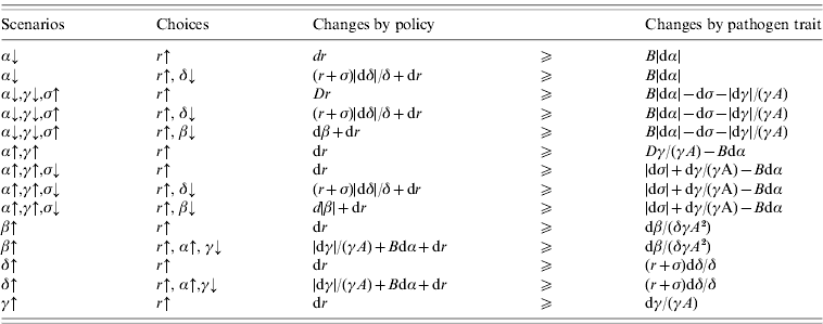
Scenarios: α↓, the duration of infection increases; α↓, γ↓, σ↑, the duration of infection increases but replication in the host (i.e. host exploitation) and consequent shedding decreases, survival in environment decreases; α↑, γ↑, the duration of infection decreases but replication in the host and consequent shedding increases; α↑, γ↑, σ↓, the duration of infection decreases but replication in the host and consequent shedding increases, survival in environment increases; β↑, frequency or intensity of host-to-host transmission increases; δ↑, frequency or intensity of environment-to-host contacts increases; γ↑, shedding rate increases.

Choices: r↑, more decontamination; r↑, δ↓, more decontamination and reduction of environment-to-host contacts; r↑, β↓, more decontamination and reduction of host-to-host contacts; r↑, α↑, γ↓, more decontamination and antibiotics administration and the consequent shedding reduction.

|·| Represents the magnitude of the differential; A=1/(r+σ+δN) and B=(β+δγA)/(αδγA ²).

Note that these criteria are not always feasible. For instance, small values of α (i.e. α≪1) imply that B≫1, where B=(β+δγA)/(αδγA ²). Then, concerning the first row of Table 2, any small decrease in the value of α must be compensated for with a large increase in the value of r, which might be impractical. In this case when (r+σ)/δ≫1, changing the control measure to the second row of Table 2 may improve the situation. In practice, after estimating the parameter values and determining the changes in infection dynamics (e.g. the scenarios presented in the first column of Table 2), the costs and feasibility of different control policies are compared and determined based on the decision criteria (e.g. those presented in Table 2).

The co-planar angle θ between the vectors ▽R ₀ and dℓ is defined by

(19)

$\theta \equals {\rm arccos}{{{\rm d}R_{\setnum{0}} } \over {\left\vert {\nabla R_{\setnum{0}} } \right\vert\left\vert {{\rm d}{\bf \ell\hskip -3.9pt\ell\hskip -3.85pt\ell} } \right\vert}}.\hfill$

The value of θ∊[0, π] is a measure of effectiveness of each control policy. When θ=π, dR ₀<0 and it has the highest magnitude. This corresponds to the policies that are most effective and the value of R ₀ is expected to decrease the most. In terms of reducing the value of R ₀, the policies become less effective when θ decreases within the range [π/2, π]. When θ=π/2, dR ₀=0, which represents a case that control policies can only prevent increases in the value of R ₀. Values of θ in the range [0, π/2) correspond to cases when the policies cannot sufficiently reduce the number of infected hosts and the value of R ₀ increases. To demonstrate the above-mentioned qualities, consider the example of E. coli O157:H7. Using the same parameter values as in Figure 3 and letting r=0·2 we obtain R ₀=0·99, A=3·145 and B=8·38. Assuming that the recovery rate α decreases by 15% (i.e. dα=−7·2×10⁻³ and α=0·0408) will increase the value of R ₀ to 1·17. To overcome the negative impacts of α on R ₀ we may increase the level of decontamination. Then the decision criterion in the first row of the Table 2 will be equivalent to dr>0·06, which means that the level of daily decontamination must increase by a minimum of 30% to return R ₀ to its previous value. An increase of 30% in the daily decontamination level could be impractical and we may have to look for an alternative approach. If we assume that the environment-to-host contacts can be reduced by 10%, then the decision criterion in the second row of Table 2 will be equivalent to dr>0·028. This will improve the situation and reduce the minimum requirement for decontamination from 30% to 14%. When such increases (i.e. 30% and 14%) are applied to the level of decontamination, the value of θ becomes π/2. This indicates that the policies are successful in preventing any increases in R ₀ above 0·99, but they cannot further decrease such values unless higher levels of decontamination are applied.

DISCUSSION

The role of environmental contamination in infection transmission is host–pathogen–environment system specific. Ideally, the nature of the organizing principle that underlies the systems should be revealed. In practice, parsimonious models can be used to understand key elements of infectious disease dynamics. Here, we used a SIS _p model to investigate the effectiveness of ED in controlling disease spread in a host population.

The main findings of the present work are divided into three parts: equilibrium analysis of the SIS _p model, impacts of ED on disease dynamics and the effectiveness of control policies. The equilibrium analysis of the SIS _p model indicates the presence of two distinct dynamics. A DF equilibrium which is stable when R ₀<1; and an unstable DF and stable E equilibria when R ₀>1. In the latter case, the E equilibrium is globally stable in the region I<I*, in which the host population is susceptible to infection. The bifurcation analysis of the SIS _p model indicates that ED can be a determining factor for reduction of infection only when the recovery rate α is in the range specified by equation (15). In this case the host population returns to a disease-free state when the level of decontamination maintains r>r ₀. On the contrary, when α is outside of the specified range, a DF equilibrium is not achievable. In particular, condition (15) can be violated when the host-to-host transmission rate β is increased. Therefore the efficiency of ED is largely dependent on β. In other words, large values of β imply $R_{{\setnum{0}}_d}$ >1. Then the eradication of infection will not be achieved and ED will only have a diminishing return in terms of reducing the number of infected hosts I* at E equilibrium. The efficiency of each control policy was quantified through a differential technique. The decision criteria in Table 2 indicate the minimal effort that is required to overcome the increases in R ₀ due to changes in the pathogen–host–environment system. Moreover, in terms of the magnitude of changes in R ₀, the value of θ is a measure of effectiveness corresponding to each intervention. While the hypothesized scenarios are not all inclusive, they illustrate the ED effort that would be required to, for example, eliminate from a host population a newly introduced or evolved strain of an infectious agent. The practical utility of this method depends on our ability to measure and distinguish the routes of disease transmission and accurately estimate other model parameters. This could be challenging for newly emerging infectious diseases. However, for a variety of infections, it is possible to obtain reasonable values for the transmission rates β and δ and other model parameters. If the changes in the parameter values of the model are detected early enough, then the correct control policy can be chosen to stop or significantly slow down the spread of infection in the host population.

As outlined below, the SIS _p model carries a number of limitations and the effectiveness of ED can be quantified and investigated for the extended versions of the model. First, no demographic stochasticity is considered in the SIS _p model [21]. Second, the model does not consider any seasonal forcing for parameters such as transmission rates β and δ or shedding rate γ (see [Reference Altizer36] for a review on seasonal impacts of β). Third, the host and pathogen population can be divided into more detailed subpopulations [Reference Ayscue17, Reference Brauer, van den Driessche and Jianhong21]. Despite these points for improvement, the analysis of the SIS _p model is conceptually meaningful for real-world scenarios in prevention and control of many historical and emergent diseases and in assessment of ED effectiveness. As mentioned in the Introduction there are controversial results and opinions regarding the effectiveness of ED. The controversy in assessment of ED effectiveness arises from the specificities of the pathogen–host–environment interactions; for example cholera transmission will be different in urban and rural settings and may become extremely different in case of a natural disaster. This could be resolved by analysing host–pathogen–environment models of infectious diseases and determining specific conditions for effectiveness of ED. For instance, with the specific parameter values related to typhoid fever and E. coli O157:H7, condition (15) is satisfied and our model predicted that ED would eradicate both cases. Alternatively, for larger values of β or N, condition (15) would be violated and ED may have a diminishing return such that for r⩾r _max ED becomes totally ineffective. Furthermore, the SIS _p model can be extended to study the effectiveness of ED in more detail. Specifically, the spatial movement of individuals, displacement of pathogens in the environment, the intermittent shedding [Reference Ivanek23], and the replication of free-living pathogens could be added to the model. Then the SIS _p is extended to an SIS reaction-diffusion model [Reference Brauer, van den Driessche and Jianhong21] with a free-living pathogen to further quantify the effectiveness of ED.

The qualitative behaviours (i.e. parabolic, linear, constant) of $R_{\setnum{0}_{d} }$ and $R_{\setnum{0}_{{in}} }$ with respect to each parameter of the SIS _p model provide crucial information for control and prevention of infection. If a parameter associated with a pathogen trait increases R ₀ linearly, then neutralizing such an increase with parameters that parabolically decrease R ₀ could be difficult when these parameters are away from zero. For instance, in a community with no or poor decontamination policies, applying higher levels of decontamination can greatly reduce the value of $R_{\setnum{0}_{{in}} }$ and therefore R ₀. Noting that ED has no effect on $R_{\setnum{0}_{d} }$ , and that it has a diminishing return in terms of reducing the value of $R_{\setnum{0}_{{in}} }$ , there is less benefit in applying higher levels of decontamination for the communities that already have a good or average decontamination policy.

In general, considering that R ₀ is defined as a function of parameters used in an epidemiological model of disease transmission, the condition R ₀<1 can be equivalent to certain conditions for some controllable parameters of the SIS _p model such as host-to-host transmission rate β, decontamination rate r and recovery rate α. This has been noted in the work by Safan et al. [Reference Safan, Heesterbeek and Dietz37], where the minimal effort required for eradicating infection is obtained for the class of compartmental models with backward bifurcation. The parameter changes that we considered in this study (i.e. Table 2) do not represent all possible cases. Nevertheless, the same technique can be employed to obtain the related decision criteria.

In conclusion, by using a simple model we determined the key elements in control of infection when ED is used as a measure. Furthermore, we illustrated how effectiveness of different control policies and ED can be quantified. This knowledge might be of special interest to healthcare professionals and decision makers, as it helps determine the feasibility of ED and the effort required to control or eliminate infection from a host population.

ACKNOWLEDGEMENTS

This work was supported by the National Science Foundation grant NSF-EF-0913367 to R.I. funded under the American Recovery and Reinvestment Act of 2009. Any opinions, findings, and conclusions or recommendations expressed in this material are those of the authors and do not necessarily reflect the views of the National Science Foundation.

APPENDIX A. Local stability analysis of the model

In the following we will show that: (i) the DF equilibrium is locally (but not asymptotically) stable when condition (8) is satisfied, (ii) the system exhibits a transcritical bifurcation when condition (8) is violated [i.e. stability of DF equilibrium is lost and at the same time the locally (and globally) stable positive E equilibrium emerges], and (iii) the solutions curves nearby the DF and E equilibria are monotonic.

The Jacobian matrix associated with the SIS _p model (1)–(3) linearized about the equilibrium (S _i, I _i, P _i), i=DF, E is given by

(20)

$J_{\lpar S_{i} \comma I_{i} \comma P_{i} \rpar } \equals \left[ {\matrix{ { \minus \beta I_{i} \minus \delta P_{i} } \tab { \minus \beta S_{i} \plus \alpha } \tab { \minus \delta S_{i} } \cr {\beta I_{i} \plus \delta P_{i} } \tab {\beta S_{i} \minus \alpha } \tab {\delta S_{i} } \cr { \minus \delta P_{i} } \tab {\gamma \minus \delta P_{i} } \tab { \minus \lpar r \plus \sigma \plus \delta N\rpar } \cr} } \right].$

Then, the characteristic equation corresponding to DF equilibrium (S _DF, I _DF, P _DF)=(N, 0, 0) is in the form

(21)

$\eqalign{ \tab \lambda \lpar \lambda ^{\setnum{2}} \plus \lpar \alpha \plus r \plus \sigma \plus \lpar \delta \minus \beta \rpar N\rpar \lambda \cr \tab\quad \plus \lpar \alpha \minus \beta N\rpar \lpar r \plus \sigma \plus \delta N\rpar \minus \gamma \delta N\rpar \equals 0\comma \cr}$

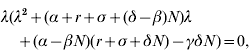
where λ is an eigenvalue. Hence, one of the eigenvalues is zero and the stability of DF equilibrium cannot be asymptotic. Employing the Routh–Hurwitz criteria (see e.g. [Reference Allen22]), the two remaining eigenvalues have negative real parts if

(22)

$N\lpar \beta \plus \delta \gamma \sol \lpar r \plus \sigma \plus \delta N\rpar \rpar \sol \alpha \lt 1.$

Note that this is the same as condition (8) for non-existence of E equilibrium. When condition (22) is satisfied, DF equilibrium is stable and it is the only equilibrium of the SIS _p model (1)–(3). In fact, condition (22) guarantees the two eigenvalues to be real negative values. Hence, the behaviour of solution curves [S(t), I(t), P(t)] is monotonic nearby the DF equilibrium.

In the case that the inequality in condition (22) is reversed, E equilibrium exists and following the same procedure, the corresponding characteristic equation is given by

(23)

$\lambda \lpar \lambda ^{\setnum{2}} \plus b\lambda \plus c\rpar \equals 0\comma$

where

(24)

$b \equals \alpha \plus \delta P\ast \plus \beta \lpar I{ \ast } \minus S{ \ast } \rpar \plus r \plus \sigma \plus \delta N\comma$

and

(25)

$c \equals \lpar r \plus \sigma \plus \delta N\rpar {{\alpha I{ \ast } } \over {S{ \ast } }}.$

Note that I*=N−S*; moreover, S* and P* are given in equations (6) and (7). Similar to the previous case, the stability is not asymptotic and we need b, c⩾0 to have a general stability. Since α – βS=ΔS*P*/I* and S*, I*, P*>0, we have b>0. Also c>0 is already satisfied. We can see that b ² −4 c>0, hence all eigenvalues are real and non-positive. Therefore the solutions near E equilibrium are monotonic and there will be no oscillations in the values of S(t), I(t) and P(t).

APPENDIX B. Global stability of E equilibrium

Here we show that E equilibrium is globally stable in the region I<I*.

Noting that the system (1)–(3) can be reduced to the system (2)–(3) by replacing S with N − I, we are required to construct a Liapunov function V(I, P) which satisfies global stability conditions. In particular, define

(26)

$V\lpar I\comma P\rpar \equals \lpar N \minus I\rpar ^{\setnum{2}} \minus \lpar N \minus I{ \ast } \rpar ^{\setnum{2}} \comma$

where I<I*.

Clearly, V*(I*, P*)=0; V(I, P)>0 for all I<I*. Moreover, using I*=N−S* and equation (6) it can be shown that

(27)

${{{\rm d}V} \over {{\rm d}t}}\lpar I\comma P\rpar \equals \lpar \dot{I}\comma \dot{P}\rpar.\nabla V\lpar I\comma P\rpar \lt 0\comma$

for all I<I*. Thus, by Liapunov's stability theorem (see section 2·9 of [Reference Perko38]), E equilibrium is a global attractor in the region that I<I*.

APPENDIX C. The basic reproduction number

The specified forms of F and V ⁻¹ are given by

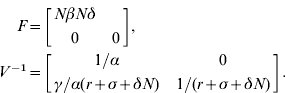
$\eqalign {F \tab\equals \left[ {\matrix{ {N\beta } {N\delta } \cr 0 \tab 0 \cr} } \right]\comma \cr V^{ \minus \setnum{1}} \tab\equals \left[ {\matrix{ {1\sol \alpha } \tab 0 \cr {\gamma \sol \alpha \lpar r \plus \sigma \plus \delta N\rpar } \tab {1\sol \lpar r \plus \sigma \plus \delta N\rpar } \cr} } \right].$

The entries (1, 1) and (1, 2) of F are the rates of secondary infections produced in compartment I by an infected host and the free-living pathogen, respectively. Since compartment P only consists of the free-living pathogen, there is no infection produced in P and therefore the second row of F is zero. The entries (1, 1) and (2, 2) of V ⁻¹ represent the average durations of time an infected host and pathogen spend in compartments I and P, respectively. The entry (1, 2) of V ⁻¹ is zero since the individuals in compartment I are already infected and therefore the pathogen does not have any impact on them. The entry (2,1) of V ⁻¹ represents a product of the rate of pathogens generated by an infected host per unit time γ and the average duration of time that each individual pathogen remains in the environment 1/α(r+σ+δN). The next-generation matrix K=FV ⁻¹ is given by

$K \equals \left[ {\matrix{ {N\beta \sol \alpha \plus N\delta \gamma \sol \lpar r \plus \sigma \plus \delta N\rpar \alpha } \tab {N\delta \sol \lpar r \plus \sigma \plus \delta N\rpar } \cr 0 \tab 0 \cr} } \right].$

The entries (1, 1) and (1, 2) of K are the expected numbers of secondary infections in compartment I produced by infected hosts and pathogen, respectively.

DECLARATION OF INTEREST

None.

References

REFERENCES

1.Boone, SA, Gerba, CP. Significance of fomites in the spread of respiratory and enteric viral disease. Applied and Environmental Microbiology 2007; 73: 1687–1696.CrossRef Google Scholar PubMed

2.Pelletier, PA, du Moulin, GC, Stottmeier, KD. Mycobacteria in public water supplies: Comparative resistance to chlorine. Microbiological Sciencs 1988; 5: 147–148.Google Scholar PubMed

3.Manangan, LP, et al. Infection control dogma: top 10 suspects. Infection Control and Hospital Epidemiology 2001; 22: 243–247.CrossRef Google Scholar PubMed

4.Scott, E, Bloomfield, SF. The survival and transfer of microbial contamination via cloths, hands, and utensils. Journal of Applied Bacteriology 1990; 68: 271–278.CrossRef Google Scholar PubMed

5.Centers for Disease Control and Prevention. Draft guideline for environmental infection control in healthcare facilities, 2001 (http://www.cdc.gov/ncid/hip/enviro/guide.htm). Accessed 7 March 2010.Google Scholar

6.International Scientific Forum on Home Hygiene. The need for a home hygiene policy and guidelines on home hygiene (http://www.ifh-homehygiene.org/public/keynote/keyn000c.htm). Accessed 15 June 2001.Google Scholar

7.Boyce, JM, et al. Environmental contamination due to methicillin-resistant Staphylococcus aureus: possible infection control implications. Infection Control and Hospital Epidemiology 1997; 18: 622–627.CrossRef Google Scholar PubMed

8.Caraco, T, Wang, IN. Free-living pathogens: life-history constraints and strain competition. Journal of Theoretical Biology 2008; 250: 569–579.CrossRef Google Scholar PubMed

9.Anderson, RM, May, RM. Infectious diseases of humans: Dynamics and control, Oxford and New York: Oxford University Press, 1991.CrossRef Google Scholar

10.Godfray, HCJ, OReilly, DD, Briggs, CJ. A model of nucleopolyhedrovirus (NPV) population genetics applied to coocclusion and the spread of the few polyhedra (FP) phenotype. Proceedings of the Royal Society of London, Series B 1997; 264: 315–322.CrossRef Google Scholar

11.Evans, HF, Entwistle, PF. Viral diseases. In Fuxa, JR, Tanada, Y, eds. Epizootiology of Insect Diseases. New York: Wiley & Sons, 1987, pp. 257–322.Google Scholar

12.Cozad, A, Jones, RD. Disinfection and the prevention of infectious disease. American Journal of Infection Control 2003; 31: 243–254.CrossRef Google Scholar PubMed

13.Food and Drug Administration Retail Food Program Steering Committee. Report of the FDA retail food program database of foodborne illness risk factors, 10 August 2000.Google Scholar

14.Rutala, WA. Disinfection, sterilization, and waste disposal. In: Wenzel, RP, ed. Prevention and Control of Nosocomial Infections. Baltimore, MD: Williams & Wilkins, 1997, pp. 539–593.Google Scholar

15.Maki, DG, et al. Relation of the inanimate hospital environment to endemic nosocomial infection. New England Journal of Medicine 1982; 307: 1562–1566.CrossRef Google Scholar PubMed

16.Daschner, F, Schuster, A. Disinfection and the prevention of infectious disease: No adverse effects? American Journal of Infection Control 2004; 32: 224–225.CrossRef Google Scholar PubMed

17.Ayscue, P, et al. Modeling on-farm Escherichia coli O157:H7 population dynamics. Foodborne Pathogens and Disease 2009; 6: 461–470.CrossRef Google Scholar PubMed

18.Boots, M. A general host-pathogen model with free-living infective stages and differing rates of uptake of the infective stages by infected and susceptible hosts. Researches on Population Ecology 1999; 41: 189–194.CrossRef Google Scholar

19.Gonzalez-Guzman, J. An epidemiological model for direct and indirect transmission of typhoid fever. Mathematical Biosciences 1989; 96: 33–46.CrossRef Google Scholar PubMed

20.Turner, J, et al. A model appropriate to the transmission of a human food-borne pathogen in a multigroup managed herd. Preventive Veterinary Medicine 2003; 57: 175–198.CrossRef Google Scholar

21.Brauer, F, van den Driessche, P, Jianhong, Wu (eds). Mathematical Epidemiology. Lecture Notes in Mathematics. Berlin Heidelberg: Springer-Verlag, 2008.CrossRef Google Scholar

22.Allen, LJS. An Introduction to Mathematical Biology. New Jersey: Pearson-Prentice Hall, 2006.Google Scholar

23.Ivanek, R, et al. Markov chain approach to analyze the dynamics of pathogen fecal shedding – example of Listeria monocytogenes shedding in a herd of dairy cattle. Journal of Theoretical Biology 2007; 245: 44–58.CrossRef Google Scholar

24.Diekmann, O, Heesterbeek, JAP. Mathematical Epidemiology of Infectious Diseases, Wiley Series in Mathematical and Computational Biology. West Sussex, England: John Wiley & Sons, 2000.Google Scholar

25.Chowell, G, Brauer, F. The basic reproduction number of infectious diseases: Computation and estimation using compartmental epidemic models. In: Chowell, G, et al. eds. Mathematical and Statistical Estimation Approaches in Epidemiology. New York: Springer, 2009, pp. 1–30.CrossRef Google Scholar

26.van den Driessche, P, Watmough, J. Reproduction numbers and sub-threshold endemic equilibria for compartmental models of disease transmission. Mathematical Biosciences 2002; 180: 29–48.CrossRef Google Scholar PubMed

27.Diekmann, O, Heesterbeek, JAP, Roberts, MG. The construction of next-generation matrices for compartmental epidemic models. Journal of the Royal Society Interface 2010; 7: 873–885.CrossRef Google Scholar PubMed

28.Tien, JH, Earn, DJ. Multiple transmission pathways and disease dynamics in a waterborne pathogen model. Bulletin of Mathematical Biology 2010; 72: 1506–1533.CrossRef Google Scholar

29.Chapagain, P, et al. A mathematical model of the dynamics of Salmonella Cerro infection in a US dairy herd. Epidemiology and Infection 2008; 136: 263–272.CrossRef Google Scholar

30.Hota, B. Contamination, disinfection, and cross-colonization: are hospital surfaces reservoirs for nosocomial infection? Clinical Infectious Diseases 2004; 39: 1182–1189.Google Scholar PubMed

31.Mechie, SC, Chapman, PA, Siddons, CA. A fifteen month study of Escherichia coli O157:H7 in a dairy herd. Epidemiology and Infection 1997; 118: 17–25.CrossRef Google Scholar

32.Cray, WC, et al. Effect of dietary stress on fecal shedding of Escherichia coli O157:H7 in calves. Applied and Environmental Microbiology 1998; 64: 1975–1979.CrossRef Google Scholar PubMed

33.Bolton, DJ, et al. The survival characteristics of a non-toxigenic strain of Escherichia coli O157:H7. Journal of Applied Microbiology 1999; 86: 407–411.CrossRef Google Scholar PubMed

34.Anderson, RM, May, RM. Infectious diseases and population cycles of forest insects. Science 1980; 210: 658–661.CrossRef Google Scholar PubMed

35.Bonhoeffer, S, Lenski, R, Ebert, D. The curse of the pharaoh: The evolution of virulence in pathogens with long living propagules. Proceedings of the Royal Society of London, Series B 1996; 263: 715–721.Google Scholar PubMed

36.Altizer, S, et al. Seasonality and the dynamics of infectious diseases. Ecology Letters 2006; 9: 467–484.CrossRef Google Scholar PubMed

37.Safan, M, Heesterbeek, H, Dietz, K. The minimum effort required to eradicate infections in models with backward bifurcation. Journal of Mathematical Biology 2006; 53: 703–718.CrossRef Google Scholar PubMed

38.Perko, L. Differential Equations and Dynamical Systems, 3rd edn. New York: Springer-Verlag, 2001.CrossRef Google Scholar

Fig. 1.A schematic representation of the SISp model. Solid and dashed lines indicate the dynamics of host and free-living pathogen, respectively.

Table 1.Summary of the notations used in the model

Fig. 2.Depending on the intensity of host-to-host transmission rate β, a more aggressive environmental decontamination may increase the number of susceptibles S* (and therefore decrease the number of infected host I*) at endemic equilibrium. The diminishing return of r on S* (and therefore I*) is replaced with a linear relationship as β→0.

Fig. 3.Illustration of the effectiveness of environmental decontamination for two infectious diseases. Plots on the left- and right-hand sides correspond respectively to Escherichia coli O157:H7 in cattle and typhoid fever in humans. (a, b) Bifurcation diagrams with respect to the parameter r. The minimal daily pathogen removal required for elimination of endemic equilibrium are 18% and 73%, respectively, which is obtained from \lpar 1 \minus {\rm e}^{ \minus r_{\setnum{0}} } \rpar \times 100. (c, d) Plots of changes in R0 with respect to the decontamination level for E. coli O157:H7 and typhoid fever. The parameter values used to generate the diagrams are as follows. For E. coli O157:H7 and typhoid fever, respectively, N=100, 100; α=0·048, 0·0357; β=10−4, 1·1992×10−4; δ=3×10−13, 1·8396×10−5; γ=4×108, 18·5822; σ=0·118, 0·1425; r0=0·1978 and r0=1·2975. DF, Disease free; E, endemic.

Fig. 4.A conceptual illustration of the parabolic and linear changes in the value of R0 as a result of parameter changes. (a) An increase of δ results in a parabolic increase in the value of R0, whereas increases in γ give rise to parabolic decreases in R0. (b) Comparison with the previous case, since α is present both in R_{\setnum{0}_{d} } and R_{\setnum{0}_{{in}} } , it has impacts stronger than γ in controlling the increases in R0. (c) The value of R0 is linearly increased with parameters β and γ. (d) Similar to r and α, the parameter σ has a diminishing return in controlling the linear increases in R0 due to increases in β or δ.

Table 2.Hypothesized scenarios of pathogen trait changes and the policy choices to control those changes. Each inequality represents the decision criterion required to ensure the policy will be effective

Article contents

Effectiveness of environmental decontamination as an infection control measure

Summary

Keywords

Information

INTRODUCTION

THE MODEL

EQUILIBRIUM AND ECOLOGICAL STABILITY

Equilibrium analysis

The basic reproduction number

DISEASE CONTROL AND MANAGEMENT

Reduction of infection

Elimination of infection

Examples: Escherichia coli O157:H7 and typhoid fever

Impacts of parameter changes

Control of pathogen trait changes

DISCUSSION

ACKNOWLEDGEMENTS

APPENDIX A. Local stability analysis of the model

APPENDIX B. Global stability of E equilibrium

APPENDIX C. The basic reproduction number

DECLARATION OF INTEREST

References

REFERENCES

Save article to Kindle

Save article to Dropbox

Save article to Google Drive

Reply to: Submit a response

Your details

You have entered the maximum number of contributors

Conflicting interests