1. INTRODUCTION
Multi-system integration is an effective method to improve system performance in terms of integrity, accuracy and continuity. The Kalman filter has been widely applied in multi-sensor integration application for decades. It is an effective and versatile method to estimate the state from uncertain dynamics by combining the noisy sensor outputs. Nevertheless, the state estimation of a Kalman filter, whatever sensor outputs are used, has to face the nonlinearity of the state space model (Yang et al., Reference Yang, Cui and Gao2004). The Extended Kalman Filter (EKF) and Linearized Kalman Filter (LKF) are approaches to deal with the nonlinearity of the model. The filters both use analytical methods to approximate the nonlinear functional model. They employ the first order Taylor series expansion to approximate the nonlinear equations and estimate the state with the Kalman Filter afterwards. EKF linearizes the state space model about the estimated trajectory which is continuously updated from the measurements (Brown and Hwang, Reference Brown and Hwang2012). LKF linearizes the model about the precompiled nominal trajectory, which does not depend on the measurement data. The linearization process of EKF and LKF, however, inevitably introduces linearization errors as the higher order terms of the expansion are ignored. The linearization accuracy of LKF also depends on the predetermined nominal trajectory. The inaccurate nominal trajectory leads to filter instability. Another type of model to handle the nonlinearity is to approximate the state probabilistic distribution rather than to linearize the nonlinear function. The Particle Filter (PF) is a representative method and uses a sequential Monte Carlo sampling method based on a Bayesian theorem to approximate the posterior Probability Density Function (PDF) of the system state. The optimal estimation of the nonlinear and non-Gaussian state space model is provided by a large quantity of samples (Rigatos, Reference Rigatos2012; Arulampalam et al., Reference Arulampalam, Maskell, Gordon and Clapp2002; Gustafsson et al., Reference Gustafsson, Gunnarsson, Bergman, Forssell, Jansson, Karlsson and Nordlund2002). The method selects a finite number of random samples based on assumed probability distribution and propagates them through a nonlinear function. The transformed samples accurately reflect the statistical properties of the system of interest. The balance between efficiency and accuracy is the main obstacle in real time operation.
The Unscented Kalman Filter (UKF), introduced by Julier and Uhlmann (Reference Julier and Uhlmann1997), is another probabilistic approach to approximate the state distribution by Gaussian random variables. The filter utilises the Unscented Transformation (UT) to estimate the system state which undergoes a nonlinear transformation (Julier and Uhlmann, Reference Julier and Uhlmann2004; Wan and Van der Merwe, Reference Wan and Van der Merwe2000). In contrast to a PF, UKF requires only a minimal set of samples, namely the sigma points, to propagate through the nonlinear equation. The predicted mean and covariance are calculated accurately by the transformed sigma points at least to the second order of Taylor expansion (Julier, Reference Julier2002; Gustafsson and Hendeby, Reference Gustafsson and Hendeby2012). Different sampling strategies of sigma points have been proposed to improve the estimation efficiency (Julier, Reference Julier1998; Reference Julier2002; Reference Julier2003; Julier and Uhlmann, Reference Julier and Uhlmann2002; Zhang et al., Reference Zhang, Liu and Zhao2009). The symmetric sampling method has the best estimation accuracy among the strategies. The bound radius of the sigma points, however, affects the estimation accuracy. The Scaled Unscented Transformation (SUT) is an approach to reduce the spread of the sigma points and decrease the nonlocal effect in state estimation (Julier, Reference Julier2002; Van der Merwe, Reference Van der Merwe2004).
Comparative studies among the filters have been carried out in recent years. Researchers have used a radar tracking simulation to compare the performance of the three filters, PF, EKF and UKF. This shows that the filters have similar performance within a mild nonlinear environment (Wan et al., Reference Wan, Liu and Pi2007). Similar results were achieved in an orbit determination scenario and attitude estimation of a flight test (Gaebler et al., Reference Gaebler, Hur-Diaz and Carpenter2014). LaViola (Reference LaViola2003) carried out a comparison between EKF and UKF in human motion tracking for virtual reality applications. The study concluded that UKF has the same performance as EKF, but requires additional computation capacity. Spacecraft localisation based on angular measurement simulation shows that both EKF and UKF are able to achieve the desirable accuracy, while UKF performs better in terms of accuracy and consistency of the estimation (Giannitrapani et al., Reference Giannitrapani, Ceccarelli, Scortecci and Garulli2011).
The above mentioned studies analysed the performance of UKF and EKF in different applications. In this paper, three cases are presented to compare the performance of UKF and EKF within the land vehicle navigation domain. The filters are compared with different feedback modes; open loop mode and closed loop mode. In the first case, a constant vehicle turning simulation is applied, which simulates the vehicle turning behaviour with a constant angular rate. The simulated on board sensors are integrated with measurements within an open loop mode. In the second case, a field test is conducted in Hong Kong, in which the Inertial Measurement Unit (IMU) is integrated with the Global Positioning System (GPS) with closed loop mode. An error model is used to build the system state model. The output of the filter is applied to mitigate the sensors’ error. In the third case, a field test is carried out in Beijing, in a suburban environment. In the test, the GPS raw measurements are integrated with a constant velocity model with a tightly coupled integration approach.
In the next section, the algorithms and the relationships of UKF and EKF are presented. Three case studies are analysed in Section 3. The conclusions are drawn in Section 4.
2. THE KALMAN FILTERING FRAMEWORK
2.1. General State Space Model
The system state estimation problem is a special case of the Bayesian framework and the system can be described by a state space model. The model depicts the probabilistic dependence between the latent state variable and the observed measurements (Chen and Brown, Reference Chen and Brown2013), and can be stated as,
 $$x_k = f\left( {x_{k - 1},w_k} \right)$$
 $$y_k = h\left( {x_k,e_k} \right)$$
where f and h are either linear or nonlinear equations. f is the transition equation of state evolution and h is the observation equation; k is a discrete time index; x k is the n-dimensional system state at epoch k; y k is the observation vector; w k and e k are process noise and observation noise vectors, respectively.
The recursive Bayesian estimation first predicts the system state based on current information and the system evolution equation, and updates the predicted information based on the noisy measurements (Orderud, Reference Orderud2005). The prediction stage propagates the current state distribution through the function f, and then the predicted PDF is obtained,
 $$p\left( {x_k \vert y_{k - 1}} \right) =\ \int p\left( {x_k \vert x_{k - 1}} \right)p\left( {x_{k - 1} \vert y_{k - 1}} \right)dx_{k - 1}$$
where the term
 $p\left( {x_k \vert x_{k - 1}} \right)$
is the probability model of the state evolution specified by the function f and the process noise distribution
 $p\left( {w_k} \right)$
. The update stage corrects the predicted PDF by the latest measurements via a Bayesian rule (Rigatos, Reference Rigatos2012),
 $$p\left( {x_k \vert y_k} \right) = \displaystyle{{\,p(y_k \vert x_k)p(x_k \vert y_{k - 1})} \over {\,p(y_k \vert y_{k - 1})}}$$
where the normalising constant
 $$p\left( {y_k{\rm \vert} y_{k - 1}} \right) =\ \int p\left( {y_k{\rm \vert} x_k} \right)p\left( {x_k{\rm \vert} y_{k - 1}} \right)dx_k$$
depends on the likelihood function
 $p\left( {y_k{\rm \vert}x_k} \right)$
which is fully specified by the observation function h and the observation noise distribution
 $p\left( {e_k} \right)$
.
2.2. The Kalman Filter
The general form of the Bayesian approach is difficult for analytical calculation as the denominator of Equation (4) cannot be computed analytically (Doucet et al., Reference Doucet, Godsill and Andrieu2000; Doucet et al., Reference Doucet, de Freitas and Gorden2001). The Kalman Filter, however, can be applied to approximate the posterior PDF of the state, if the state space model is linear.
In reality, however, the system state space models are usually described by the nonlinear equations. The Kalman Filter then estimates the system state by linearizing the nonlinear equation with the first order Taylor series expansion about the estimated state, namely the Extended Kalman Filter. EKF has been widely accepted as a standard method in dealing with multiple sensor fusion (Grejner-Brzezinska and Yi, Reference Grejner-Brzezinska and Yi2003; Wu and Yang, Reference Wu and Yang2010). The linearized state space model can then be written as,
 $$x_k = Fx_{k - 1} + w_{k - 1}$$
 $$y_k = Hx_k + e_k$$
where F is the linear dynamic transition matrix and H is the observation design matrix. The Kalman Filter estimation flow is,
 $$\bar x_k = F\hat x_{k - 1}$$
 $$P_{{\bar x}_k} = FP_{{\hat x}_{k - 1}}F^T + P_{w_k}$$
 $$\hat x_k = \bar x_k + K_k\left( {y_k - H{\bar x}_k} \right)$$
 $$K_k = P_{{\bar x}_k}H^T\left( {HP_{{\bar x}_k}H^T + P_{e_k}} \right)^{ - 1}$$
 $$P_{{\hat x}_k} = \left( {I - K_kH} \right)P_{{\bar x}_k}\left( {I - H^TK_k^T} \right) + K_kP_{e_k}K_k^T $$
where
 $\bar x_k$
is the predicted system state vector at epoch k;
 $\hat x_{k - 1}$
is the estimated state vector at the last epoch and
 $P_{{\hat x}_{k - 1}}$
is the corresponding covariance matrix;
 $P_{w_k}{\rm \;} $
and
 $P_{e_k}$
are the covariance matrices of process noise and observation noise, respectively. The subscript k is time instant.
EKF analytically propagates the state covariance matrix through the linearized state space model. The linearization process requires the calculation of the Jacobian matrix, which increases the calculation complexity and inevitably introduces linearization errors.
2.3. The Unscented Kalman Filter
UKF estimates the state posterior PDF based on the Kalman Filtering framework by approximating the state probability distribution, whereas EKF approximates the nonlinear function. It is easier to approximate a probability distribution than to approximate a nonlinear function (Julier and Uhlmann, Reference Julier and Uhlmann1997; Huang and Wang, Reference Huang and Wang2006; Rambabu et al., Reference Rambabu, Bjarne and Lars2008). The UKF samples a set of sigma points to match the current statistics properties and then propagates the points through the nonlinear function. The predicted mean and covariance are then estimated by the weighted transformed sigma points (Julier and Uhlmann, Reference Julier and Uhlmann1997; Cui et al., Reference Cui, Hong and Layne2005).
The sigma points are chosen based on the estimated state covariance matrix with deterministic method,
 $$\eqalign{{\hat x}_{0,k - 1} & = {\hat x}_{k - 1} \cr {\hat x}_{i,k - 1} & = {\hat x}_{k - 1} + \gamma S_i \qquad i = 1,2, \cdots, n \cr {\hat x}_{i + n,k - 1} & = {\hat x}_{k - 1} - \gamma S_i}$$
where n is the dimension of the augmented state vector and γ is a scale factor,
 $$\gamma = \sqrt {n + \kappa} $$
where the parameter κ fine tunes the sigma points. It affects the third and higher order terms of the Taylor expansion. It is possible to match some of the fourth order terms when the state vector is Gaussian if κ = 3 − n. S i is the ith row or column of the square root of the state covariance matrix,
 $$S_i = \sqrt {P_{{\hat x}_{k - 1}}} _i$$
 $P_{{\hat x}_{k - 1}}$
is the state covariance matrix, and i is the ith column of the matrix square root.
The predicted state,
 $$\bar x_{i,k} = f\left( {{\hat x}_{i,k - 1}} \right)$$
 $$\bar x_k = \mathop \sum \limits_{i = 0}^{2n} \left( {w_i{\bar x}_{i,k}} \right)$$
where w i is the weight of the sigma points,
 $$\eqalign{w_0 &= {\displaystyle{\kappa \over {N + \kappa}},}\quad\ \qquad {i = 0} \cr w_i &= {\displaystyle{\kappa \over {2(N + \kappa )}},} \qquad {i \ne 0} \cr}$$
where N is the number of the sigma points, N = 2n + 1.
The predicted covariance matrix can be calculated by the weighted transformed sigma points and the approximated mean,
 $$P_{{\bar x}_k} = P_{w_k} + \mathop \sum \limits_{i = 0}^{2n} w_i\left( {{\bar x}_{i,k} - {\bar x}_k} \right)\left( {{\bar x}_{i,k} - {\bar x}_k} \right)^T$$
The predicted measurement
 $\bar y$
and corresponding covariance are,
 $$\bar y_{i,k} = h\left( {{\bar x}_{i,k}} \right)$$
 $$\bar y_k = \mathop \sum \limits_{i = 0}^{2n} w_i\bar y_{i,k}$$
 $$P_{{\bar y}_k} = P_{e_k} + \mathop \sum \limits_{i = 0}^{2n} w_i\left( {{\bar y}_{i,k} - {\bar y}_k} \right)\left( {{\bar y}_{i,k} - {\bar y}_k} \right)^T$$
The cross-correlated covariance is,
 $$P_{{\bar x}_k{\bar y}_k} = \mathop \sum \limits_{i = 0}^{2n} w_i\left( {{\bar x}_{i,k} - {\bar x}_k} \right)\left( {{\bar y}_{i,k} - {\bar y}_k} \right)^T$$
The Kalman gain in UKF is written as,
 $$K_k = P_{{\bar x}_k{\bar y}_k}P_{{\bar y}_k}^{ - 1} $$
The estimated state vector is,
 $$\hat x_k = \bar x_k + K_k\left( {y_k - {\bar y}_k} \right)$$
and the estimated covariance is,
 $$P_{{\hat x}_k} = P_{{\bar x}_k} - K_kP_{{\bar y}_k}K_k^T $$
2.4. Theoretical Relations between Extended and Unscented Kalman Filter
UKF flow is similar to that of EKF as aforementioned. Nevertheless, the cross covariance matrix of UKF is approximated by the sigma points, as illustrated in Equation (23). The following equation can be derived on the assumption that the state space model is linear,
 $$\eqalign{P_{{\bar x}_k{\bar y}_k} & = E\left( \left( {\bar x}_k - E\left( {\bar x}_k \right) \right) \left({\bar y}_k - E\left({\bar y}_k \right) \right)^T \right) \cr & = E \left( \left({\bar x}_k - E\left( {\bar x}_k \right) \right) \left( H{\bar x}_k - E\left( H{\bar x}_k \right) \right)^T \right) \cr & = E\left(\left({\bar x}_k - E\left( {\bar x}_k \right) \right)\left({\bar x}_k - E\left( {\bar x}_k \right) \right)^T H^T \right) \cr & = P_{{\bar x}_k}H^T}$$
Thus, EKF and UKF have the same significance of Kalman gain, that is,
 $$K_{EKF} = P_{{\bar x}_k}H^T\left( {HP_{{\bar x}_k}H^T + P_{e_k}} \right)^{ - 1} = P_{{\bar x}_k{\bar y}_k}P_{{\bar y}_k}^{ - 1} = K_{UKF}$$
From the derivations and state estimators, some theoretical relationships between UKF and EKF can be found in state estimation with nonlinear models:
-
(1) Both UKF and EKF operate within the Kalman Filtering framework. The accuracy of the estimated state depends on the predicted state
 $\bar x_k$
, and predicted measurement
$\bar y_k$
as well as the Kalman gain matrix.
-
(2) UKF has better prediction accuracy than EKF in the most nonlinear state cases. The state mean and covariance matrix of UKF are obtained by the weighted sigma points propagated through the nonlinear function. The propagated process, Unscented Transformation, avoids introducing the linearization error, which decreases the filter performance.
-
(3) The predicted measurement constructs the innovation vector, which affects the accuracy of the final estimation. The accuracy of the predicted measurement
$\bar y_k\; $
in UKF is more accurate than that of EKF. UKF approximates the predicted measurements with the sigma points via the system dynamic model and then the observation model. The first propagation receives system predicted state, as mentioned in point (2). The second propagation, the transformed sigma points propagating through the nonlinear observation model, obtains the predicted measurements. Nevertheless, the EKF acquires the predicted measurements through the linearized models, system model and observation model, which introduces the linearization error in both predictions. -
(4) The reliability of the estimated state
$\hat x_k\; $
relies on the Kalman gain matrix K
k
. EKF calculates the Kalman gain by using the predicted covariance matrices
$P_{{\bar x}_k}$
and
$P_{e_k}$
as well as the linearized design matrix H
k
. The linearization error exists in all three items as mentioned above. UKF, however, obtains the cross covariance matrix
$P_{{\bar x}_k{\bar y}_k}{\rm \;} $
and the predicted measurement covariance matrix
$P_{{\bar y}_k}$
by weighted sigma points. The points can be used to calculate the projected mean and covariance correctly to the second order (Julier and Uhlmann, Reference Julier and Uhlmann2004). -
(5) Compared with EKF, the Jacobian matrix of the nonlinear equation is not needed in the UKF estimation process.
-
(6) UKF propagates the sigma points through the nonlinear function iteratively, which are related with the dimension of the system state vector, while EKF only requires calculating the Jacobian matrix once.
-
(7) UKF calculates the square root of the state covariance matrix to sample the sigma points with the aim of matching the current statistic properties. The Cholesky decomposition is an effective method to perform the square root of a positive-definite matrix (Agarwal and Mehra, Reference Agarwal and Mehra2014). The decomposition, however, requires the numerical stability of the process, since the iteration of UKF cannot always guarantee the production of a positive-definite matrix.


The performance comparison of prediction of UKF and EKF is presented by the following example.
 $$\eqalign{y_1 & = x_1\sin \theta \cr y_2 & = x_2\cos \theta} $$
The system state is denoted by
 $X = \left[ {\matrix{ x & y & \theta \cr}} \right]^T$
, with its covariance matrix
 $P = 1*10^{ - 2}*diag\left( {\left[ {\matrix{ {{\left( {1m} \right)}^2} & {{\left( {1.414m} \right)}^2} & {{\left( {3m} \right)}^2} \cr}} \right]} \right)$
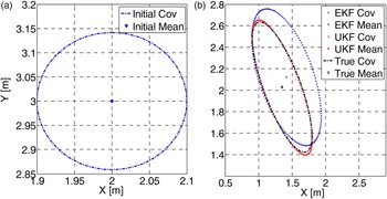
. In Figure 1, the initial state mean and covariance are shown in Figure 1(a), and the predicted information is shown in Figure 1(b). The Monte Carlo approaches with 107 samples are used to provide the reference information and they are shown with a dot-dash line in Figure 1(b). The 1-σ error ellipse is used to present the error bound of the estimated states. UKF estimated results close to the reference, while the mean of EKF is biased and the covariance ellipse is enlarged and biased. The Root Mean Square Error (RMSE) is presented in Table 1.
The performance comparison of Unscented and Extended Kalman Filters.

Comparison of RMSE [m].

2.5. The Scaled Unscented Transformation (SUT)
Unscented Transformation is the key technique of UKF. It determines sigma points to match the current statistical properties. The sampling strategy of the sigma points is not unique. Symmetric sampling, minimal skew sampling and spherical simplex sampling are very popular methods. The symmetric sampling approach is widely used as it has the best estimation accuracy (Orderud, Reference Orderud2005). The bound radius of the sigma points is related to the state dimension. The increased state dimension will also increase the bound radius of the sigma points, which may introduce the nonlocal effect. That is, the filter may not guarantee the positive semi-definite of the matrix (Julier, Reference Julier1998). SUT is proposed to scale the bound radius of the sigma points to overcome the nonlocal effect. The approach is presented below,
 $$\eqalign{& \chi _i = \,{\hat x}_{k - 1}\, \pm \,\sqrt {(n + \lambda )p_{\hat x}} _{k - 1_i} \cr & W_0^{({\rm m})} \, = \,\displaystyle{\lambda \over {n + \lambda}} \cr & W_0^{({\rm c})} \, = \,\displaystyle{\lambda \over {n + \lambda}} \, + (1 - \alpha ^2 + \beta ) \cr & W_{i\,}\, = \,\displaystyle{1 \over {2(n + \lambda )}} \cr & \lambda = \,\alpha ^2\,(n + \kappa )^{ - n}} $$
where 0 ≤ α ≤ 1 is the scale factor which determines the bound radius of the sigma points; if the state is Gaussian, then β = 2; κ ≥ 0 to guarantee positive semi-definiteness of the covariance matrix. W i is the weight that associates with ith sigma point, and the superscript m and c represent the mean and covariance, respectively. The details of the derivations can be found in Gustafsson and Hendeby (Reference Gustafsson and Hendeby2012).
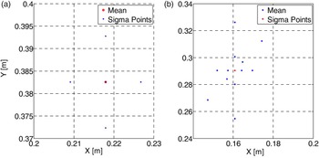
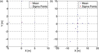
The scaled and the non-scaled symmetric sampling approaches are presented in Figures 2 and 3, respectively. The approaches propagate the sigma points through the same system transition function. The parameters of scaled symmetric sampling are set as, α = 0.01, β = 2, κ = 0.
The Scaled Unscented Transformation.

The Unscented Transformation.

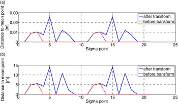
Figure 2(a) and Figure 3(a) are the initial state mean and sigma points. The transformed sigma points and the approximated mean are presented in Figure 2(b) and 3(b). The distances from the sigma points to the mean position are illustrated in Figure 4.
The distances from the sigma points to the mean point.

Figure 4 presents the spread of the sigma points before and after propagation though the nonlinear equation with respect to
 $\hat x_{0,k - 1}$
and
 $\bar x_{0,k}$
, respectively.
 $\hat x_{0,k - 1}$
is the estimated state at epoch k − 1;
 $\bar x_{0,k}$
is its prediction via the nonlinear model. The spread of sigma points in SUT is noticeably smaller relative to that in UT, as shown in Figure 4(a) and 4(b). UT inevitably introduces nonlocal effects to the estimation of the system state. It is also found that the spread of sigma points in SUT is determined by α. The spread of SUT is the same as that of UT when α = 1. In this research SUT is considered in the system state estimation.
3. CALCULATION AND COMPARISON BY USING SIMULATED AND ACTUAL DATA
To comprehensively evaluate the filters’ effectiveness and to verify the theoretical differences between UKF and EKF, three different case studies, including a simulation test and two field tests, are carried out within the vehicle navigation application domain. The simulation and the field test data are processed in the Matlab R2010a 64-bit program on a PC with Intel Core i7–3770 CPU at 3·40 GHz, 16-GB RAM equipped with Windows 7.
The first case simulates a vehicle constant turning behaviour with an open loop mode. The second test was carried out in Hong Kong. GPS and IMU are integrated with a loosely coupled strategy. The estimated errors are fed back to compensate the IMU sensors. The third test was conducted in Beijing. The GPS observations and a constant velocity model were constructed to form a tightly coupled integration system. The cases are intended to analyse the effectiveness of the approaches through the different state space models and feedback modes, with EKF and UKF.
3.1. Case 1: Open Loop Constant turn Model
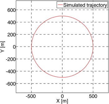
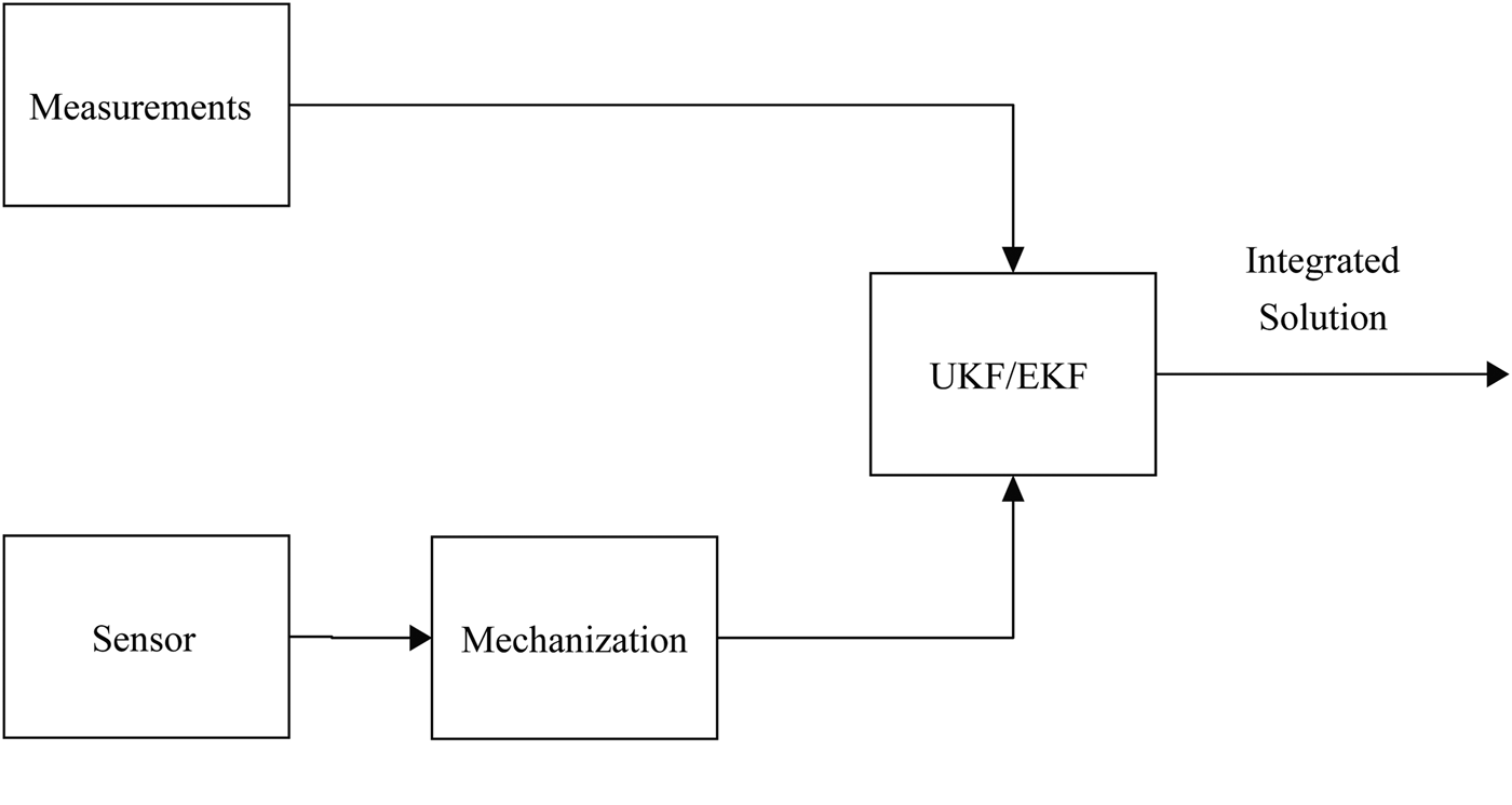
Constant turning is a behaviour where a vehicle is turning with a constant angular rate ω. Thus a nonlinear dynamic model with respect to vehicle heading velocity is used to describe the system. The simulation assumes the vehicle conducts a constant turning at a constant angular rate of 2·54°/s with a heading velocity of 81 km/h. The vehicle is constrained on a 500 m radius. The designed trajectory is shown in Figure 5. The system mechanisation model is employed to predict the state. The on board sensors sense the states every 0·1 s. The observations are assumed to be updated every 1 s. The simulation duration is 141 s. It can be observed from Figure 6 that with the open loop mode, the estimated states are directly used in mechanisation at the next epoch.
True vehicle trajectory.

Open Loop Implementation of Filter Integration.

The discrete dynamic model with the state vector is,
 $$f\,(x_k y_k v_{k\,\,} \omega _k \theta _k) = \left[ {\matrix{ {x_{k - 1\,} - v_{k - 1\,\,}t\sin \,\theta _{k - 1}} \cr {y_{k - 1\,} - v_{k - 1\,\,}t\cos \,\theta _{k - 1}} \cr {v_{k - 1}} \cr {\omega _{k - 1}} \cr {\theta _{k - 1} - \omega _{k - 1}t} \cr}} \right] + w_{k - 1}$$
where x
k
, y
k
describe vehicle position in a two-dimensional coordinate system; v
k
is heading velocity; ω
k
is the vehicle's angular velocity; and θ
k
is vehicle heading; w
k−1 is Gaussian noise with zero mean and covariance matrix
 $P_{w_{k - 1}}$
; the subscript k indicates time instant k. The observation function states as,
 $$L_k = H_kX_k + e_k$$
where H
k
is an identity matrix, and e
k
is the uncorrelated observation noise with covariance matrix
 $P_{e_k} = diag\left[ {{\left( {1m} \right)}^2\; {\left( {1m} \right)}^2\; {\left( {0.5m/s} \right)}^2\; {\left( {0.001rad/s} \right)}^2\; {\left( {0.01rad} \right)}^2} \right]$
. The initial states are set as
 $X = \left[ {\matrix{ {\matrix{ {498.93} & { - 0.94} \cr}} & {22.62} & {\matrix{ {0.045} & { - 0.016} \cr}} \cr}} \right]^T$
.
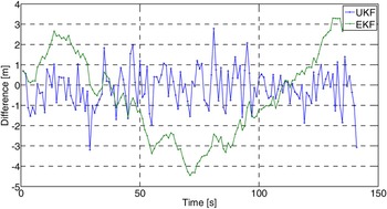
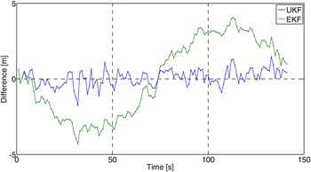
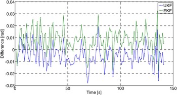
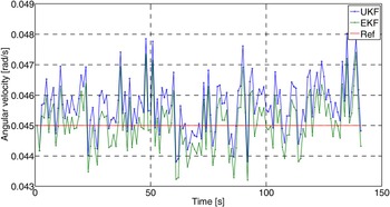
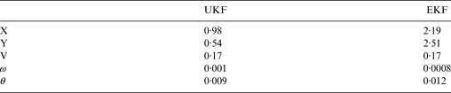
The performance of UKF and EKF are compared with respect to the simulated value. In Figures 7 and 8, the errors of the X and Y components are presented. Figure 9 presents the vehicle heading error. Vehicle angular velocities are presented in Figure 10, the reference angular velocity is presented in red. The RMSE at filter epoch of UKF and EKF are listed in Table 2.
Estimation Error of X component.

Estimation Error of Y component.

Estimated Vehicle Heading Error.

Estimated Angular Velocities (the reference angular velocity is presented in red colour).

RMSE at Filter Epoch [m].

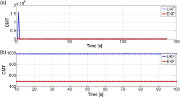
The trace of the predicted covariance matrix is presented in Figure 11. Figure 11(a) shows the predicted state covariance matrix trace (CMT) estimated by UKF and EKF, respectively; the difference between two estimators is presented in Figure 11(b) from epoch 10 to 100 s.
Predicted Covariance matrix trace of Unscented and Extended Kalman Filters.

The above results show that:
-
(1) The result of UKF estimation is more accurate than that of EKF through using nonlinear models. The RMSE of UKF for X component is 0·98 m and 0·54 m for Y component with respect to the simulated true position. EKF achieved 2·19 m and 2·51 m RMSE for X and Y components, respectively.
-
(2) From Figure 11, it is apparent that the trace of predicted state covariance matrix of UKF is larger than that of EKF,
$tr\left( {P_{{\bar x}_k}^{UKF}} \right) \gt tr\left( {P_{{\bar x}_k}^{EKF}} \right)$
. Thus, UKF is less affected by the historical information, which leads the estimation close to the observation.

3.2. Case 2: Closed loop GPS/IMU Integrated Navigation System
In this case, a field test was conducted in Hong Kong. The vehicle was driven through a dense building area with many overpasses and viaducts. Its position is represented in the Hong Kong 80 Grid coordinate system. The vehicle was driven for about 15 minutes. The data was collected from Hitachi H48C 3-axis accelerometer and Analog Devices ADXRS300 gyroscope at 100 Hz (Hitachi, 2007; Analog Devices Inc., 2004). The accelerometer is used to sense the acceleration in the heading direction. The gyroscope measures the change of vehicle heading. A GPS module is equipped for position and velocity measurements every 1·4 s. The GPS and IMU are loosely coupled. The system provides state information in National Marine Electronics Association (NMEA) 0813 standard, including position, timing, velocity, acceleration and heading. The standard is a specification for communication between marine electronics equipment. GPS receiver communication is defined within this specification.
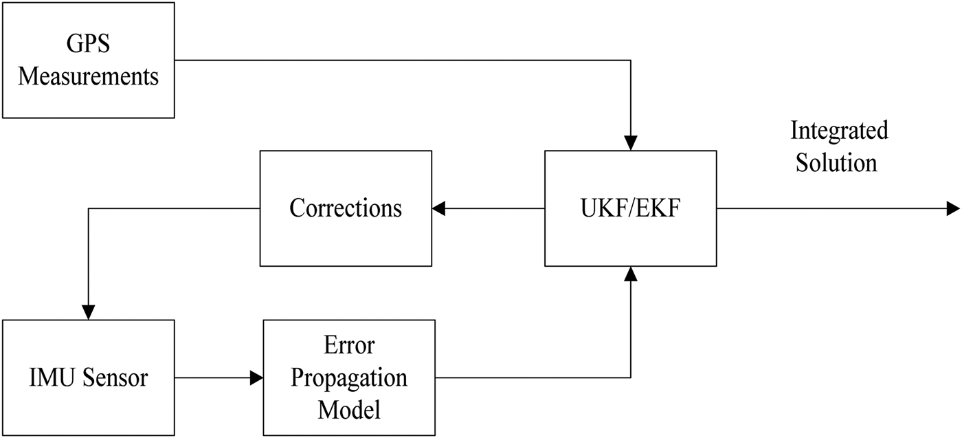
In this case, the error state is used to establish the system dynamic model. The estimated result is feedback to compensate the IMU measurements. The schematic of close loop implementation of Case 2 is shown in Figure 12. The state vector is,
 $$X = [\delta x\,\,\delta y\,\,\delta v\,\,\delta \theta \,\,b\,\,\delta \omega \,\,s]^T$$
Close Loop Implementation of UKF/EKF.

and the nonlinear dynamic model is described by the following equations.
 $$\eqalign{& X_{k + 1} = f\,(X_k) + w_k\cr &\quad = \left[ {\matrix{ {\delta x_k + \delta v_kT\sin \theta _k + v_kT\cos \theta _k\, \cdot \delta \theta _k + 0.5\delta a_kT^2\sin \theta _k + 0.5a_kT^2\cos \theta _k \cdot \delta \theta _k} \cr {\delta x_k + \delta v_kT\cos \theta _k + v_kT\sin \theta _k\, \cdot \delta \theta _k + 0.5\delta a_kT^2\cos \theta _k + 0.5a_kT^2\sin \theta _k \cdot \delta \theta _k} \cr {\delta v_k + \delta a_kT} \cr {\delta \theta _k + d_kT} \cr {e^{\displaystyle{{ - T} \over {\tau _g}}}b} \cr {e^{\displaystyle{{ - T} \over {\tau _g}}}\delta \omega} \cr {e^{\displaystyle{{ - T} \over {\tau _g}}}s} \cr} \,} \right]\cr & \qquad+ W_k}$$
where δx and δy are positioning errors; δv is the vehicle velocity error with respect to heading direction; δθ is the vehicle heading error; b is acceleration bias; δω is the angular rate difference; s is the scale factor of accelerometer; τ
g
is the relevant time constant of the accelerometer and the gyroscope; T is the time interval. The system noise information is defined as W
k
= [0 0 0 0 w
b
w
δω
w
s
]
T
and considered as white noise with a covariance matrix
 $P_{w_k}$
.
The observation equation is,
 $$y_k = H_kX_k + e_k$$
where H k is the design matrix,
 $$H_k = \left[ {\matrix{1 & 0 & 0 & 0 & 0 & 0 & 0 \cr 0 & 1 & 0 & 0 & 0 & 0 & 0 \cr 0 & 0 & 1 & 0 & 0 & 0 & 0 \cr 0 & 0 & 0 & 1 & 0 & 0 & 0 \cr}}\right]$$
y k is the measurements vector with noise vector e k ,
 $$y_k = \left[ {P_{gps} - P_{INS},V_{gps} - V_{INS},Head_{GPS} - Head_{INS}} \right]^T$$
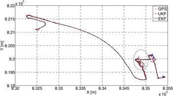
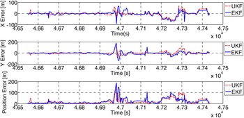
The estimated positions with UKF and EKF are presented with GPS measurements in Figure 13. The positioning errors with respect to GPS measurements for X, Y components and the overall position errors are depicted in Figure 14. The dash line stands for UKF estimation and the solid line for the EKF estimation. The RMSE of UKF and EKF are listed in Table 3.
Vehicle Trajectory.

Positioning Error of UKF and EKF.

Comparison of RMSE [m].

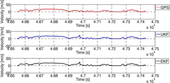
Peak values in Figure 14 correspond to the marked area in Figure 13. The number of the visible satellites in that area is less than four. Figure 15 presents the vehicle velocity measured by GPS, and the estimation of UKF and EKF.
Velocity Estimated by GPS, Unscented and Extended Kalman Filters.

In the test, UKF yields equal or slightly better accuracy in state estimation when compared with EKF. The reason is that the error model moderates the nonlinearity of the state space model. The estimated result of UKF is closer to the measurements than that of EKF, even if the measurements are contaminated.
3.3. Case 3: Constant Velocity Model
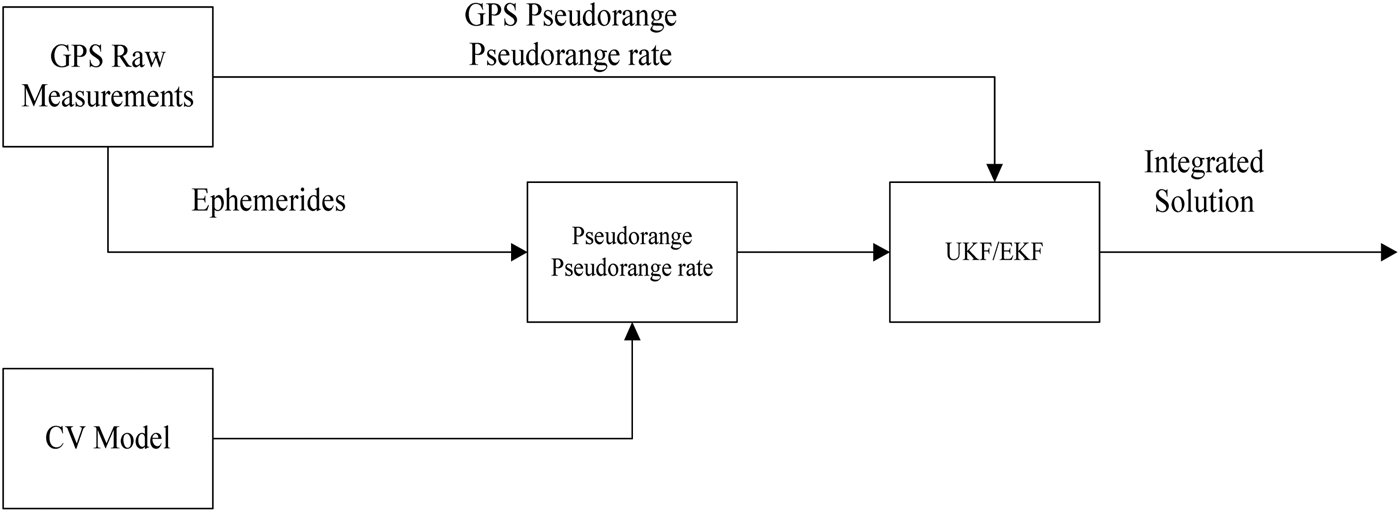
In this case, the test was conducted on Beijing's Fifth Ring Road, a suburban environment. The GPS receiver was equipped to collect the vehicle position and velocity with 1 s data rate. The driven time was about 3 hours. The constant velocity model is used as the system dynamic model to predict the state. The predicted position and velocity are transferred to the GPS observation model, which is a nonlinear model with raw GPS measurements, to predict the observed pseudorange and pseudorange rate. The integration architecture is presented in Figure 16. The state vector is
 $X = \left[ {x,y,z,v_x,v_y,v_z,\delta t,\delta \dot t} \right]^T$
, where [x, y, z]
T
are vehicle coordinates in the WGS84 coordinate system; [v
x
, v
y
, v
z
]
T
are the corresponding velocity components; δt is the receiver clock bias, and
 $\delta \dot t$
is the clock bias rate. The system observes the pseudorange and Doppler shift directly. The observation vector is
 $L_k = \left[ {\rho _i,{\dot \rho} _i} \right]^T$
, where ρ
i
is the pseudorange of ith satellites and
 $\dot \rho _i$
is its Doppler shift. The initial states are zero.
Block Diagram of Integration Strategy.

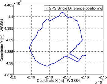
The vehicle trajectory measured by GPS single difference approach is illustrated in Figure 17. The carrier phase measurements are used as the reference.
Vehicle Trajectory.

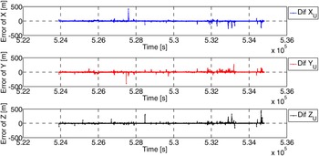
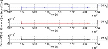
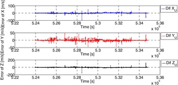
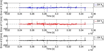
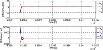
The error of estimated position with respect to carrier phase measurements is shown in Figures 18 and 19. The RMSE of position estimation is listed in Table 4. The error of estimated velocity with respect to the GPS Doppler measurement is plotted in Figures 20 and 21. Convergence time of UKF and EKF with respect to the single difference positioning approach is shown in Figure 22.
UKF positioning error with respect to GPS single difference approach.

EKF positioning error with respect to GPS single difference approach.

Velocity error of UKF with respect to the GPS Doppler measurement.

Velocity error of EKF with respect to the GPS Doppler measurement.

The convergence time of UKF and EKF.

The RMSE of UKF and EKF with respect to GPS carrier phase measurement (m).

With zero initial states, UKF converges faster than EKF. The two approaches, however, have no resistance to the outliers of observations (i.e. multipath effect of the GPS observations). The test results of three cases again confirmed that UKF performs better than EKF in terms of accuracy and consistency.
4. CONCLUSIONS
In this paper, the performance of UKF with scaled unscented transformation and EKF for vehicle navigation has been analysed in three cases. The vehicle state has been estimated via UKF and EKF using different state space models. The behaviour of the filters has been verified with different feedback modes and integration strategies. In the open loop, the nonlinear equations act as the system model, and are easy to implement. In the closed loop mode, the error model is used as the system dynamic model. The process of acquiring the model moderates the nonlinearity of the equations. The accuracies of both estimators are acceptable. The UKF has shown better performance in terms of accuracy and consistency, especially with nonlinear equations.
Some conclusions can be drawn: UKF has better performance in nonlinear state estimation. It uses the nonlinear equations to build the state space model straightforwardly, while EKF requires to linearize the model in order to propagate the state mean and covariance matrix. Therefore, UKF is easier in model design than EKF. The trace of predicted state covariance matrix of UKF is larger than that of EKF. The former is acquired through the sigma points, and the latter is propagated through the linearized model. Therefore, UKF gives less weight to historical information compared with EKF. Furthermore, the sigma points are sampled according to the updated state covariance matrix, which indicates the predicted state and covariance matrix are closely related to the updated information. The estimation process of EKF, however, is easier than UKF.