2 Measurements

The BMSW (Fast Solar Wind Monitor) instrument (Šafránková et al. Reference Šafránková, Němeček, Přech, Zastenker, Cěrmák, Chesalin, Komárek, Vaverka, Beránek and Pavlu2013b ; Zastenker et al. Reference Zastenker, Khrapchenkov, Koloskova, Gavrilova, Ryazanova, Ryazantseva, Gagua, Gagua, Šafránková and Němeček2013) on board the Spektr-R spacecraft provides measurements of plasma parameters – the ion flux value and its direction together with proton density, bulk and thermal velocities – with a time resolution of 31 ms. The instrument consists of 3 Faraday caps facing sunward (along the $X_{BMSW}$ axis) and 3 cups deviating by $20^{\circ }$ from the $X_{BMSW}$ axis. BMSW operates both in the SW and MSH, however, the full spatial distribution function is not always available in the MSH due to the limited aperture of the instrument ( $\pm 50^{\circ }$ ). Thus, the MSH plasma parameters can be calculated reliably only at the MSH flanks. Moreover, Spektr-R has a high-elliptic orbit with continuous (more than 2 h duration) MSH crossings usually taking place at the flanks. BMSW measures permanently the ion flux value and its direction with 31 ms time resolution, although measurements of ion density and velocities are not always available with the same resolution. Moreover, the method of density and velocity determination is not always valid in the MSH due to high ion temperatures in this region. However, some features of the density and velocity fluctuations can be obtained from the fluctuations of ion flux value and its direction.

The ion flux direction is characterised by the polar angle $\unicode[STIX]{x1D703}$ – the deviation of a flux vector from the $X_{BMSW}$ axis – and the azimuth angle $\unicode[STIX]{x1D711}$ measured clockwise from the $Y_{BMSW}$ axis. The BMSW instrument is equipped with the DSS (Detector of Sun Shine) sensor providing the angle between $X_{GSE}$ and $X_{BMSW}$ – $\unicode[STIX]{x1D6FC}$ . The angle $\unicode[STIX]{x1D6FC}$ varies usually within the limit of $15^{\circ }$ and changes continuously, although this change is very slow ( ${\sim}1^{\circ }$ per day). In the present study we deal with polar angle in the BMSW coordinate system to avoid noise arising due to the additional recalculation. BMSW measurements in the MSH are reliable for $\unicode[STIX]{x1D703}<25^{\circ }$ due to the increasing errors of ion flux value determination for larger angles (see Gagua, Gagua & Zastenker Reference Gagua, Gagua, Zastenker, Safrankova and Pavlu2009).

As the velocity usually varies in a less intensive manner than the density (with respect to its mean value) the ion flux fluctuations represent fluctuations of ion density. A comparison of the ion density fluctuation spectrum with the ion flux value fluctuation spectrum was presented in Pitňa et al. (Reference Pitňa, Šafránková, Němeček, Goncharov, Němec, Přech, Chen and Zastenker2016) confirming our suggestion. As density is a scalar quantity, the direction of the ion flux vector is, in fact, a characteristic of the plasma velocity. Hence, the polar angle fluctuations are affected by the fluctuations of bulk velocity rather than ion density. Thus, a deviation of the spectrum of the ion flux value from the polar angle fluctuation spectrum gives us information concerning the bulk velocity spectrum.

The BMSW is a prototype of the Faraday cup instrument (FAR) instrument on board upcoming THOR mission (Vaivads et al. Reference Vaivads2016). Results obtained from the present study are relevant for planning the mission’s goals in the MSH.

Figure 1.

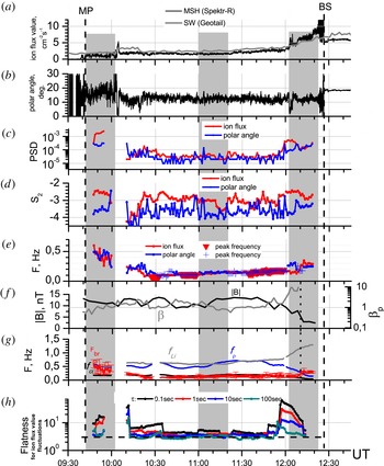
Evolution of parameters through the MSH on 9 February, 2012: (a) ion flux value in SW (grey line) and in MSH (black line); (b) MSH polar angle; (c) power spectral density (PSD) of ion flux value (here and hereafter red line) and polar angle (here and hereafter blue line) fluctuations; (d) spectral index $S_{2}$ of ion flux value and polar angle fluctuation spectra; (e) break frequency of ion flux value and polar angle fluctuation spectra and frequencies of peak (red triangles for ion flux value, blue crosses for polar angle); (f) modelled magnetic field magnitude (black line, left panel) and $\unicode[STIX]{x1D6FD}$ (grey line, right panel); (g) break frequency of the ion flux fluctuation spectrum (red line) and ion characteristic frequencies: ion cyclotron frequency (black line), gyrostructure frequency (blue line) and inertial length frequency (grey line); (h) flatness of ion flux value fluctuations.

3 Magnetosheath crossing

The flank MSH crossing under study takes place on 9 February, 2012. Spektr-R crosses the magnetopause at 09:43 at [6; 2; 10] $_{GSE}$ R $_{E}$ and enters the SW at 12:24 at [4; 4; 13] $_{GSE}$ R $_{E}$ (GSE being the Geocentric Solar Equatorial System and R $_{E}$ being the Earth’s radius). The ion flux and polar angle measurements are shown by black lines in figures 1(a) and 1(b), respectively. The ion flux value varies slightly near $2{-}3~\text{cm}^{-2}~\text{s}^{-1}$ during the whole interval and increases toward the bow shock (after 12:00 UT) up to $10~\text{cm}^{-2}~\text{s}^{-1}$ . The grey line in figure 1(a) shows the SW ion flux measured by Geotail upstream from the bow shock at [30; $-6$ ; 4] $_{GSE}$ R $_{E}$ . The SW data are shifted by the plasma propagation time ( ${\sim}480~\text{s}$ ). One can see that the increase of the MSH ion flux toward the bow shock is likely to be due to the SW ion flux increase. Polar angle varies from $17^{\circ }$ near the magnetopause to $12^{\circ }$ near the bow shock. Plasma flow is undisturbed during the whole interval except for the abrupt ion flux enhancement by $3~\text{cm}^{-2}~\text{s}^{-1}$ at 10:03–10:06 accompanied by significant rotation of the ion flux vector. The flux enhancement (although significantly prolonged) is seen both in the SW and MSH, hence, it cannot be caused by the magnetopause motion. We exclude the time interval 10:03–10:06 UT from the study because the polar angle $\unicode[STIX]{x1D703}>25^{\circ }$ . During the whole crossing, except for the eliminated interval 10:03–10:06, the angle between the bow shock normal and the interplanetary magnetic field – $\unicode[STIX]{x1D703}_{BN}$ – is larger than $45^{\circ }$ , i.e. we deal with the MSH behind the quasi-perpendicular bow shock.

Figure 2.

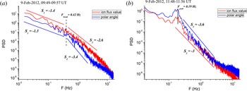
Examples of ion flux value (red line) and polar angle (blue line) fluctuation spectra: (a) that can be approximated by two power laws with sloped $S_{1}$ and $S_{2}$ divided by a break at frequency $F_{br}$ ; (b) spectra with peak at the break frequency $F_{peak}$ . Time interval used for spectra calculation is specified in each panel.

For the further analysis we divide the interval into 142 intervals with duration of 512 s (16 000 data points) and lagged by 1 min (i.e. intervals are overlapped by 452 s). In the present study we concentrate on the frequency spectra at ion kinetic scales. According to Riazantseva et al. (Reference Riazantseva, Budaev, Rakhmanova, Zastenker, Šafránková, Němeček and Přech2016) the break of ion flux fluctuation spectra in the MSH occurs at frequencies $0.9\pm 0.5~\text{Hz}$ . Thus, the number of data points in each interval is sufficient to observe and approximate the spectra above the break. We calculate the power spectral density (PSD) of the ion flux value and polar angle fluctuations for each interval using the fast Fourier transform and then smooth the spectra with a Hamming window in the frequency domain. Various types of spectral shapes of plasma fluctuations in the SW and MSH were reported previously: with two power laws separated by the break (e.g. Šafránková et al. Reference Šafránková, Němeček, Přech and Zastenker2013a ; Riazantseva et al. Reference Riazantseva, Budaev, Zelenyi, Zastenker, Pavlos, Šafránková, Němeček, Přech and Němec2015, Reference Riazantseva, Budaev, Rakhmanova, Zastenker, Šafránková, Němeček and Přech2016), with a flattening near the break (e.g. Celnikier, Muschietti & Goldman Reference Celnikier, Muschietti and Goldman1987; Chen et al. Reference Chen, Howes, Bonnell, Mozer, Klein and Bale2013, Reference Chen, Sorriso-Valvo, Šafránková and Němeček2014b ; Šafránková et al. Reference Šafránková, Němeček, Němec, Přech, Pitňa, Chen and Zastenker2015), with a peak near the break (e.g. Lacombe et al. Reference Lacombe, Belmont, Hubert, Harvey, Mangeney, Russell, Gosling and Fuselier1995). One part of the spectra obtained in the present study can be approximated with two power laws with slopes $S_{1}$ and $S_{2}$ separated with the break frequency $F_{br}$ . The example of the spectra of this type is presented in figure 2(a). We normalise the data to the mean values in order to compare two quantities. Hence, the PSD is given in relative units in figure 2 and in the further study. Starting from the break frequency $F_{br}=0.2~\text{Hz}$ , the spectrum follows ${\sim}f^{-2.6}$ for the ion flux fluctuations (red line) and ${\sim}f^{-3.4}$ for the polar angle fluctuations (blue line). Lion et al. (Reference Lion, Alexandrova and Zaslavsky2016) indicated that near the break the spectrum could be decomposed into different spectra each having its own transition feature. For this reason the extended transition range rather than the break may be observed in the frequency spectrum between the inertial and kinetic ranges. We concentrate on ion kinetic scales in this study. We consider spectral indices $F_{br}$ and $S_{2}$ . $F_{br}$ is the frequency of the break or the frequency at which the transition part of the spectrum ends (i.e. the spectrum can be approximated with the power law at higher frequencies). The slope $S_{2}$ is calculated at the whole range of frequencies between $F_{br}$ and the frequency at which the instrumental noise becomes significant. Instrument noise usually occurs at frequencies ${\sim}8{-}10~\text{Hz}$ for the ion flux value fluctuations (Šafránková et al. Reference Šafránková, Němeček, Přech, Zastenker, Cěrmák, Chesalin, Komárek, Vaverka, Beránek and Pavlu2013b ). As the polar angle is calculated with the help of 3 Faraday cups, the noise level of the polar angle fluctuations is higher. Hence, the noise grows at smaller frequencies – 3–5 Hz. This difference is clearly seen in figure 2(a): the flattening of the polar angle fluctuation spectrum at frequencies above 3 Hz is observed due to the noise. The noise of the ion flux fluctuations arises at 8 Hz in this case.

Figure 3.

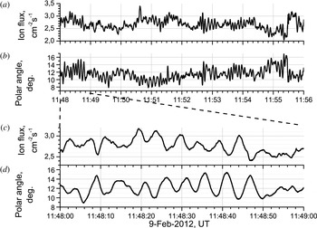
Ion flux (a and c) and polar angle (b and d) measurements on 9 February 2012. Panels (a) and (b) refer to 8-min time interval, panels (c) and (d) refer to 1-min time interval.

Another type of spectrum obtained in the present study demonstrates signatures of the instabilities. Spectra of this type occur in the middle MSH predominantly. Examples of these spectra is shown in figure 2(b). A large local maximum occurs at the frequencies comparable to the frequency of the break. Similar peaks in the magnetic field spectrum were reported by Alexandrova et al. (Reference Alexandrova, Mangeney, Maksimovic, Cornilleau-Wehrlin, Bosqued and André2006) and interpreted as the signatures of Alfvén vortices. Czaykowska et al. (Reference Czaykowska, Bauer, Treumann and Baumjohann2001) observed a similar event downstream of the quasi-perpendicular bow shock and interpreted it as a signature of AIC waves. Figure 3 shows the ion flux (panel a) and polar angle (panel b) measurements for the interval used for the spectra calculations in figure 2(b). The train of waveforms is observed in both quantities. Figures 3(c) and 3(d) show the same values during 1 min. Sinusoid-like oscillations with a period of approximately 5 s (or frequency ${\sim}0.2~\text{Hz}$ ) are observed in the plot. The ion flux value and polar angle vary in near antiphase. The peaks in the spectra occur also during 10:25–11:00 UT and 11:20–12:10 UT. Similar oscillations of electron density with frequency 0.2 Hz in the middle MSH were reported by Lacombe et al. (Reference Lacombe, Belmont, Hubert, Harvey, Mangeney, Russell, Gosling and Fuselier1995). The authors attributed these oscillations to AIC waves. The identification of the mode’s nature requires magnetic field measurements not available on board the Spektr-R spacecraft. Thus, the origin of the spectral peak is an open question.

Calculating spectra with the procedure described above we can see the time evolution of the spectral parameters with a 1 min time resolution. We distinguish 3 regions: the middle MSH (11:00–11:20 UT), the magnetopause vicinity (09:43–10:03 UT) and the bow shock vicinity (12:04–12:24 UT). The subintervals are marked in figure 1 by the shaded areas. During these subintervals the spacecraft gets over ${\sim}1R_{E}$ in the magnetopause rest frame. Figure 1(c) shows the PSD of the normalised ion flux value (red line) and polar angle (blue line) at $2\pm 0.1~\text{Hz}$ , that is, above the spectral break for all of the spectra. Each point refers to the centre of the 512 s interval used for the spectrum calculation. Power spectral density for both quantities is ${\sim}10^{-5}$ in the middle MSH, and increases towards the bow shock by an order of magnitude – to ${\sim}10^{-4}$ . In the magnetopause vicinity the PSD of the polar angle fluctuations is ${\sim}10^{-4}$ whereas the PSD of the ion flux fluctuations is higher – ${\sim}10^{-3}$ . This difference indicates that the density fluctuations are less damped near the magnetopause compared to the bulk velocity fluctuations.

Figure 1(d) presents the time evolution of $S_{2}$ for both quantities. For the ion flux fluctuations the spectra seem to be slightly steeper in the middle MSH – $S_{2}^{flux}=-3.0\pm 0.2$ – than near both of the boundaries – $S_{2}^{flux}=-2.6\pm 0.1$ . For the polar angle fluctuations $S_{2}^{angle}=-3.7\pm 0.3$ in the middle MSH and $S_{2}^{angle}=-3.4\pm 0.2$ at the boundaries. $S_{2}$ for the polar angle fluctuations are much more variable through the MSH. Despite the large standard deviations, however, one can see that $S_{2}$ for polar angle follows $S_{2}$ for ion flux value: spectra become shallower towards the boundaries. Rakhmanova et al. (Reference Rakhmanova, Riazantseva and Zastenker2016) showed that the polar angle fluctuation spectra are typically steeper than the spectra of the ion flux value fluctuations. This is also the case in the present study. The difference between the slopes is likely to be due to the difference between the density and bulk velocity fluctuation spectra at kinetic scales (see e.g. Šafránková et al. Reference Šafránková, Němeček, Přech and Zastenker2013a , Reference Šafránková, Němeček, Němec, Přech, Chen and Zastenker2016).

Huang et al. (Reference Huang, Sahraoui, Deng, He, Yuan, Zhou, Pang and Fu2014) reported $S_{2}=-2.9$ for the MSH magnetic field fluctuations above the break. This value is consistent with what is observed for ion flux fluctuations in the middle MSH. Czaykowska et al. (Reference Czaykowska, Bauer, Treumann and Baumjohann2001) reported the slope of the magnetic field fluctuations $S_{2}=-2.6$ just behind the bow shock. This slope is consistent with the one calculated for the ion flux (and hence, ion density) fluctuations near the bow shock. This result is consistent with Chen et al. (Reference Chen, Salem, Bonnell, Mozer and Bale2012b , Reference Chen, Howes, Bonnell, Mozer, Klein and Bale2013) who have reported the same spectral indices of the density and magnetic field magnitude fluctuations in the SW. The authors stressed that the coupling of the magnetic field and density fluctuations is expected in KAW turbulence. However, according to Rezeau et al. (Reference Rezeau, Belmont, Cornilleau-Wehrlin and Reberac1999) the magnetic field fluctuation spectrum has the index $S_{2}=-3.4$ in the MSH adjacent to the magnetopause. This value is considerably smaller compared to what we observe for the ion flux fluctuations in the present study. Shevyrev et al. (Reference Shevyrev, Zastenker, Eiges and Richardson2006) showed the mirror mode signatures becoming more significant when a spacecraft approaches the magnetopause. The mirror mode is of a compressive nature, hence it may be responsible for the increase of $S_{2}$ for the ion flux fluctuations towards the magnetopause.

Chen et al. (Reference Chen, Salem, Bonnell, Mozer and Bale2012b ) have reported a value of $S_{2}=-2.75\pm 0.06$ and Šafránková et al. (Reference Šafránková, Němeček, Němec, Přech, Pitňa, Chen and Zastenker2015) have reported $S_{2}=-2.6$ for the SW density fluctuation spectra. In the middle MSH the spectra of the ion flux fluctuations are steeper on average than those in the SW. Chen (Reference Chen2016) noted that the SW spectra are steeper that the predicted ones and listed several possibilities responsible for this steepening. For example, electron Landau damping leads to the spectral slope $-2.8$ (Howes et al. Reference Howes, Tenbarge, Dorland, Quataert, Schekochihin, Numata and Tatsuno2011) and accumulation of the cascade into intermittent two-dimensional structures (Boldyrev & Perez Reference Boldyrev and Perez2012) leads to the spectral slope $-8/3$ . Although closer to the in situ measurements, the spectra proposed for these processes are still shallower than those observed in the middle MSH. Thus, other mechanisms should be found that are responsible for the further steepening of the spectra in this region. For example, the anomalous steep spectra may be caused by the presence of some structures in the MSH away from the boundaries. For example, Alexandrova et al. (Reference Alexandrova, Mangeney, Maksimovic, Cornilleau-Wehrlin, Bosqued and André2006) reported the $f^{-3}$ spectrum of the magnetic field fluctuations for the interval in the MSH associated with the occurrence of Alfvén vortices.

The evolution of the spectral break frequency is shown in figure 1(e). Note that sometimes the break cannot be identified due to the peak in the fluctuation spectrum in the transition range (see figure 2 b). In figure 1(e) the frequencies of the peaks are shown by red triangles for the ion flux fluctuation spectra and by blue crosses for those of the polar angle fluctuations. For both quantities, the break frequency decreases from $0.4\pm 0.1~\text{Hz}$ in the magnetopause vicinity to $0.13\pm 0.01~\text{Hz}$ in the middle MSH and then grows slightly to $0.25\pm 0.05~\text{Hz}$ at the bow shock. Šafránková et al. (Reference Šafránková, Němeček, Němec, Přech, Chen and Zastenker2016) reported break frequencies of density and bulk velocity fluctuation spectra to be very close to each other when their frequencies are low (approximately 0.1–0.2 Hz). On the contrary, the break frequency of the velocity fluctuations is usually lower than those of density for higher frequencies of the breaks. This latter result is consistent with what we observe in the present paper: the break frequencies of the ion flux value and polar angle fluctuations are low and almost identical.

Generally, the breaks in the fluctuation spectra between MHD and ion kinetic scales are supposed to be related to ion characteristic scales – ion gyroradius $\unicode[STIX]{x1D70C}_{ci}$ , ion cyclotron frequency $f_{ci}$ or ion inertial length $L=c/\unicode[STIX]{x1D714}_{p}$ ( $\unicode[STIX]{x1D714}_{p}$ being the ion plasma frequency). Panel (g) presents the time evolution of the break frequency of the ion flux fluctuation spectrum (red line) together with the characteristic frequencies – $f_{ci}$ (black line), gyrostructure frequency $f_{\unicode[STIX]{x1D70C}}=V/2\unicode[STIX]{x03C0}\unicode[STIX]{x1D70C}_{ci}$ (blue line) and inertial length frequency $f_{L}=V/2\unicode[STIX]{x03C0}L$ (grey line); here $V$ is the plasma bulk velocity. Since magnetic field measurements are not available on board Spektr-R and there are no magnetic data from another spacecraft at the same MSH flank, we use model predictions. The BATS-R-US (Block Adaptive-Tree Solar-wind Roe-type Upwind Scheme) model (Groth et al. Reference Groth, De Zeeuw, Gombosi and Powell2000) was used with Geotail input data. The model is available on request at http://ccmc.gsfc.nasa.gov/. Plasma parameters are simulated satisfactorily for the event presented here, except for the bow shock crossing taking place 15 min before the real crossing. The resulting data row has a 120 s time resolution. The modelled magnetic field magnitude is shown in figure 1(f) (black line). The grey line in this panel shows the proton beta $\unicode[STIX]{x1D6FD}_{p}$ . The modelled bow shock is marked with the vertical dotted line in panel (g). In the middle MSH the break frequency stays close to the ion cyclotron frequency whereas near the magnetopause, the break occurs at frequencies close to the inertial length frequency and gyrostructure frequency. Breuillard et al. (Reference Breuillard, Yordanova, Vaivads and Alexandrova2016) showed the smallest of the characteristic frequencies to be the frequency of the break in the MSH magnetic field fluctuation spectrum. However, the authors also mentioned the spectrum between the smallest and the largest characteristic scale to be modified by the ion instabilities. The present paper demonstrates that in the middle MSH, the spectrum breaks at the smallest characteristic frequency $f_{ci}$ , i.e. the largest characteristic scale affects the spectrum first. This situation is consistent with the suggestions of Chen et al. (Reference Chen, Leung, Boldyrev, Maruca and Bale2014a ) in the SW. On the other hand, the increase of the break frequency near the magnetopause is not accompanied by any changes in the characteristic scales. Thus, near the magnetopause, the process leading to spectrum formation is not the one of the largest scale. One may expect that the change of the characteristic scale is due to a change of turbulence regime. The break of the magnetic fluctuation spectra at the ion cyclotron frequency was previously attributed to ion cyclotron damping (e.g. Goldstein, Roberts & Fitch Reference Goldstein, Roberts and Fitch1994). This is the case in the middle MSH. Near the magnetopause, the break is related to the ion inertial length or ion gyroradius. Hence, KAW turbulence or Hall-MHD turbulence is likely to be observed near the magnetopause. Another possible explanation is the high influence of the plasma instabilities near the magnetopause resulting in spectra modification between the characteristic scales. Sahraoui et al. (Reference Sahraoui, Belmont, Rezeau and Cornilleau-Wehrlin2006) suggested that the magnetopause prevents the turbulent cascade from developing normal to it. That is, the influence of the constraint itself may cause the change in the spectral indices observed in the present study.

Space plasma turbulence is known to be intermittent and this results in the deviation of the probability distribution function (PDF) from the Gaussian distribution (e.g. Burlaga Reference Burlaga1991; Marsch & Tu Reference Marsch and Tu1997; Sorriso-Valvo et al. Reference Sorriso-Valvo, Carbone, Veltri, Consolini and Bruno1999; Veltri Reference Veltri1999; Bruno et al. Reference Bruno, Carbone, Sorriso-Valvo and Bavassano2003; Kiyani et al. Reference Kiyani, Chapman, Khotyaintsev, Dunlop and Sahraoui2009). Intermittency of the SW plasma has been discussed with the help of the magnetic field as well as plasma measurements. Intermittency in the MSH turbulence was considered by e.g. Yordanova et al. (Reference Yordanova, Vaivads, André, Buchert and Vörös2008), Kozak et al. (Reference Kozak, Pilipenko, Chugunova and Kozak2011) with the help of magnetic field data and by Riazantseva et al. (Reference Riazantseva, Budaev, Rakhmanova, Zastenker, Šafránková, Němeček and Přech2016) and Budaev, Zelenyi & Savin (Reference Budaev, Zelenyi and Savin2015) with the help of the BMSW plasma measurements. The authors showed the PDFs of the plasma and magnetic field fluctuations exhibit heavier tails at smaller scales.

The degree of non-Gaussianity can be characterised by the flatness coefficient (Frisch Reference Frisch1995), that is defined as the fourth-order moment of the PDF $K(\unicode[STIX]{x1D70F})=S_{4}(\unicode[STIX]{x1D70F})/S_{2}^{2}(\unicode[STIX]{x1D70F})$ , where $S_{p}(\unicode[STIX]{x1D70F})=\langle (n(t+\unicode[STIX]{x1D70F})-n(t))^{p}\rangle$ . $K=3$ for a Gaussian distribution and $K>3$ for distributions with heavier tails. Figure 1(h) shows the time evolution of $K$ , calculated for the ion flux data at time scales $\unicode[STIX]{x1D70F}=0.1$ , 1, 10, 100 s. The flatness is calculated in 15 min intervals (number of points $N=28\,800$ ) to enable a reliable determination of $K$ . The intervals are lagged by 1 min from each other, points in the figure 1(h) mark the centres of the 15 min intervals. The time evolution of the flatness shows that it is strongly scale dependent near the bow shock and the magnetopause, whereas in the middle MSH its value stays near 3 for all scales. According to Frisch (Reference Frisch1995), a growth of the flatness toward smaller scales indicates intermittency in the observed flow. Thus, figure 1(h) demonstrates highly intermittent plasma flow near the MSH boundaries and low intermittent flow in the middle MSH. Comparing panels (g) and (h) one can note that in the low intermittent plasma the spectra have breaks at frequencies close to the ion cyclotron frequency whereas in the highly intermittent plasma the breaks occur at another scale. Thus, the presence of the intermittency may also influence the spectral break.

4 Summary

The magnetosheath plasma carries energy from the solar wind to the Earth’s magnetosphere. Processes taking place in the MSH should be studied not only at large scales ( ${\sim}$ Earth’s radius) but also at small scales ( ${\sim}$ ion gyroradii). The MSH plasma is turbulent and its turbulence differs from the SW turbulence because of the presence of the boundaries (e.g. Alexandrova Reference Alexandrova2008). In order to study the MSH turbulence not only the magnetic field but also plasma data are worth examining. We demonstrate an evolution of the plasma fluctuations and plasma turbulence properties across the Earth’s magnetosheath at ion kinetic scales. Our results can be summarised as follows:

1. (i) Power spectral density of the high-frequency plasma fluctuations grows toward the magnetopause and the bow shock. However, the growth rate of the PSD of the ion flux value fluctuations towards the magnetopause is higher than the growth rate of those of the polar angle fluctuations. This indicates that fluctuations of density are less damped near the magnetopause than the fluctuations of bulk velocity.

2. (ii) The slope of the kinetic-scale part of the ion flux value fluctuation spectrum changes from $-3.0\pm 0.2$ in the middle MSH to $-2.6\pm 0.1$ near the boundaries. In the bow shock vicinity the obtained values are consistent with those for magnetic field fluctuations – $S_{2}=-2.6$ – reported by Czaykowska et al. (Reference Czaykowska, Bauer, Treumann and Baumjohann2001). In the middle MSH, $S_{2}$ for the ion flux fluctuations is consistent with the one obtained in statistical study by Huang et al. (Reference Huang, Sahraoui, Deng, He, Yuan, Zhou, Pang and Fu2014). Thus, the coupling of the magnetic field and density fluctuations is observed. Similar coupling presents in kinetic Alfvén turbulence. On the contrary, in the magnetopause vicinity, the ion flux fluctuation spectrum is shallower than reported by Rezeau et al. (Reference Rezeau, Belmont, Cornilleau-Wehrlin and Reberac1999) for the magnetic field fluctuation spectrum. This may be due to uncoupling of the magnetic and density fluctuations. However, simultaneous measurements of the magnetic and density fluctuations are required to understand whether this uncoupling is a feature of the turbulence in the magnetopause vicinity. Both the ion flux value and polar angle fluctuation spectra are steeper in the middle MSH compared to the SW. The steeper spectra may be caused by the presence of structures in the MSH away from the boundaries, e.g. Alfvén vortices (Alexandrova et al. Reference Alexandrova, Mangeney, Maksimovic, Cornilleau-Wehrlin, Bosqued and André2006). The processes leading to the spectra steepening are the topic of further study.

3. (iii) The break frequency of the fluctuation spectra decreases from $0.4\pm 0.1~\text{Hz}$ in the magnetopause vicinity to $0.13\pm 0.01~\text{Hz}$ in the middle MSH and then grows slightly to ${\sim}0.25\pm 0.05~\text{Hz}$ at the bow shock for both quantities. Chen et al. (Reference Chen, Leung, Boldyrev, Maruca and Bale2014a ) and Breuillard et al. (Reference Breuillard, Yordanova, Vaivads and Alexandrova2016) reported the magnetic field fluctuation spectrum to have a break at the smallest of the characteristic frequencies. In the middle MSH, the break frequency is close to the proton gyrofrequency, which is the least of the characteristic scales in the analysed case. However, near the magnetopause, the break frequency becomes closer to the gyrostructure frequency and the inertial length frequency which are hardly distinguishable for $\unicode[STIX]{x1D6FD}\sim 1$ . Such evolution of the break frequency may be caused either by a change in the processes governing the turbulence or by the presence of the constraint – magnetopause – preventing the development of the cascade normal to it.

4. (iv) Time evolution of the level of non-Gaussianity at various time scales during the MSH crossing shows that the level of MSH plasma intermittency grows toward the boundaries. In the middle MSH non-intermittent turbulence may be observed. Yordanova et al. (Reference Yordanova, Vaivads, André, Buchert and Vörös2008) reported more intermittent turbulence at larger distances from the quasi-parallel bow shock. This discrepancy may be caused by considering the MSH behind the bow shock. Two different types of the bow shock are considered in the two papers. This may be the cause of the discrepancy between the results. Interestingly, the spectra break at the ion cyclotron frequency in the low intermittent plasma, consistent with Alfvén turbulence damped at this frequency. On the contrary, the break occurs at other scales in a highly intermittent plasma. Thus, the presence of the intermittency may affect the character of the turbulence.

5. (v) Broad peaks occur at the transition range of the spectra in the middle MSH. For these spectra clear sinusoidal oscillations with a frequency of approximately 0.2 Hz in the spacecraft frame are observed in both ion flux value and polar angle data. Previously, similar oscillations of the MSH density were reported by Lacombe et al. (Reference Lacombe, Belmont, Hubert, Harvey, Mangeney, Russell, Gosling and Fuselier1995) and were attributed to Alfvén ion cyclotron waves. Waves observed in the present study are likely to be AIC waves also, according to the $\unicode[STIX]{x1D6FD}$ values and the localisation inside the MSH.

The present study emphasises the fact that the compressive fluctuations inside the magnetosheath may differ from the fluctuations of the bulk velocity and magnetic field. Thus, density and bulk velocity fluctuations are worth studying simultaneously with the fluctuations of the magnetic field in order to catch the whole image of the processes forming the energy cascade in the magnetosheath as well as in the solar wind. The upcoming THOR mission provides an opportunity for such complex investigation. The FAR instrument suggested for THOR mission is designed on the basis of BMSW to provide high-frequency measurements of plasma parameters.