1. INTRODUCTION
The use of reflected GNSS signals as a source of opportunity for remote sensing, known as the GNSS-R technique, has been a research area of increasing interest for the past years. In the 1990's, Martin-Neira proposed the concept of the PAssive Reflectometry and Interferometry System (PARIS) (Martin-Neira, Reference Martin-Neira1993) which uses reflected GPS signals for ocean altimetry and Auber's experiment showed that scattered GPS signals from the ocean surface could be detected. Since then, in-depth research activities have been performed to enlarge the applications of this technology. Different research groups introduced their results to extract information of ocean wind (Garrison et al., Reference Garrison, Komjathy, Zavorotny and Katzberg2002, Gleason et al., Reference Gleason, Hodgart, Sun, Gommenginger, Mackin, Adjrad and Unwin2005, Zavorotny and Voronovich, Reference Zavorotny and Voronovich2000), ocean altimetry (Lowe et al., Reference Lowe, Kroger, Franklin, Labrecque, Lerma, Lough, Marcin, Muellerschoen, Spitzmesser and Young2002, Rius et al., Reference Rius, Cardellach and Martin-Neira2010, Rivas and Martin-Neira, Reference Rivas and Martin-Neira2006), sea state (Marchan-Hernandez et al., Reference Marchan-Hernandez, Valencia, Rodriguez-Alvarez, Ramos-Perez, Bosch-Lluis, Camps, Eugenio and Marcello2010, Sabia et al., Reference Sabia, Caparrini and Ruffini2007, Xin et al., Reference Xin, Qiang, Xunxie, Daren, Lianjun, Xiong, Giulio, Stephen and Soulat2008), sea ice (Komjathy et al., Reference Komjathy, Maslanik, Zavorotny, Axelrad and Katzberg2000, Rivas et al., Reference Rivas, Maslanik and Axelrad2010, Wiehl et al., Reference Wiehl, Legr'esy and Dietrich2003) and soil moisture (Katzberg et al., Reference Katzberg, Torres, Grant and Masters2006, Masters et al., Reference Masters, Axelrad and Katzberg2004, Rodriguez-Alvarez et al., Reference Rodriguez-Alvarez, Bosch-Lluis, Camps, Vall-Llossera, Valencia, Marchan-Hernandez and Ramos-Perez2009) from reflected GNSS signals through theoretical studies and experimental data analysis. However, a standard GPS receiver normally cannot access the necessary information of both direct and reflected signals. The development of special instruments that can process reflected GNSS signals has been carried out (Garrison et al., Reference Garrison, Komjathy, Zavorotny and Katzberg2002, Lowe et al., Reference Lowe, Kroger, Franklin, Labrecque, Lerma, Lough, Marcin, Muellerschoen, Spitzmesser and Young2002a, Marchan-Hernandez et al., Reference Marchan-Hernandez, Camps, Rodriguez-Alvarez, Bosch-Lluis, Ramos-Perez and Valencia2008, Meehan et al., Reference Meehan, Esterhuizen, Franklin, Lowe, Munson, Robison, Spitzmesser, Tien and Young2007, Nogués-Correig et al., Reference Nogués-Correig, Gali, Campderros and Rius2007) and several near-Earth experiments have been conducted.
In 2004, the first delay-mapping receiver (DMR) in China was developed by the authors' research group using the Zarlink GP2021/GP2010 chipset and several airborne experiments were performed to collect useful primitive data for ocean wind retrieval (Yang et al., Reference Yang, Zhang, Lu and Zhang2008). Since 2006, the GRrSv.2, which is able to perform both ground and aircraft-based GPS-reflection remote sensing, has been developed. It can output real-time remote-sensing data for ocean remote sensing, altimetry, soil moisture monitoring or other future applications with the following advanced features:
• complex (in-phase and quadrature) DDMs are computed every 1 ms, which contain both power and phase information;
• the DDMs are navigation-bit compensated and can be further processed by means of both coherent and incoherent integration with selectable integration time;
• the high resolution of DDMs both in code delay (up to 1/80 chip) and Doppler shift (up to 5 Hz) can provide a finer observation over the reflective surface and can also improve the accuracy and stability of the output DDMs;
• both the size and resolution of the DDMs and the number of satellites processing simultaneously are dynamically reconfigurable according to different application scenes;
• the Field Programmable Gate Array (FPGA) based signal processing architecture makes the system readily adaptable to utilise navigation satellite systems other than GPS, i.e. GLONASS, Galileo and Compass.
Verification experiments of both ocean and land reflection have been performed since 2009. Further analysis of experiment results shows the availability of the designed system.
2. ARCHITECTURE AND COMPONENTS
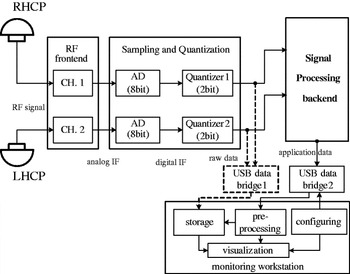
The detailed block diagram of the GRrSv.2 is designed as shown in Figure 1. There are five main blocks: the signal receiving antennas, the dual-channel RF front-end, the sampling and quantisation unit, the signal processing back-end and the monitoring workstation.
Block diagram of the GRrSv.2 architecture.

2.1. Antennas
There is a right-hand circularly polarized (RHCP) antenna for direct signal and a left-hand circularly polarized (LHCP) antenna for reflected signal. The RHCP antenna is a commercially available product. The LHCP antenna is designed as a 2×2 antennas array to equipoise gain and coverage for both land and airborne conditions. The four antenna elements can be phased and combined to produce a high-gain of 13 dB over a wide beam-width of 38°, which make the reflected GNSS signals over the whole glistening zone able to be collected with an increased SNR.
2.2. RF Front-End
The dual-channel RF front-end with symmetrical structure is applied to down-convert both direct and reflected signals synchronously. The RF signals received by the antennas are amplified, filtered and down-converted to intermediate frequency (IF) with a central frequency of 46·42 MHz.
2.3. Sampling and Quantization
The analogue IF signals are sampled by a 2-channel 8-bit A/D converter at a frequency of 20·456 MHz and quantised to 2-bit (±1 and ±3). The quantisation level is self-adaptive to guarantee the percentage of ±1 and ±3 at about 25% and 75% on average. These raw signal samples can be collected by the GNSS-R data acquisition subsystem and post-processed by a software receiver. Some primary campaigns for GNSS-R raw data collection have been performed and post-processing results verified the performance of both antennas and RF front-end (Yang et al., Reference Yang, Wang, Lu, Li and Li2010).
2.4. Signal Processing Back-End
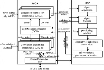
The signal processing back-end is based on the FPGA-DSP hybrid architecture, the block diagram and signal processing scheme is shown in Figure 2. FPGA based correlation channels are designed for both direct (CHD) and reflected signals (CHR). The correlation channels for reflected signal are specially designed to schedule the two-dimensional correlation. Carrier and C/A code replica for both direct and reflected signals are also generated synchronously to accommodate the synchronisation method of the reflected signals. The DSP processor is responsible for the acquisition and tracking of the direct signal and calculating the satellite-receiver geometry. Moreover, the navigation bit wrapping of the DDM is also implemented by extracting the polarity of the in-phase correlation component of the direct signal (ID).
Block diagram and signal processing scheme of the signal processing back-end.

2.5. Data Output, Pre-processing and Monitoring
The signal processing back-end computes the complex DDMs every 1 ms and other application data such as GPS time, status of available GPS satellite, information of reflective geometry and parameters (C/N0, time delay and Doppler offset) of both direct and reflected signal. These data are packaged and delivered to the monitoring workstation through the USB data bridge.
The complex DDMs can be stored in raw format or pre-processed prior to the storage by the monitoring workstation. The pre-processing of the raw DDM includes:
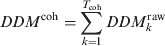
• coherent integration of the raw DDM DDM kraw during the intervals T coh,
(1)
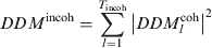
• incoherent integration of the coherent integrated DDM DDM Icoh during the intervals T incoh.
(2)
Both the coherent and incoherent integration times are configurable. The maximum coherent integration time is not limited within 20 ms because of the navigation data bit wrapping in the signal processing back-end. The status of the receiver and application data are monitored using a graphical user interface (GUI) executed in the monitoring workstation and the configurable settings can also be configured through the GUI.
3. SIGNAL PROCESSING ISSUES OF THE REFLECTED SIGNAL
The reflected GNSS signal is composed of several contributions with different time delays and Doppler offsets from different Earth surface cells, so the properties of reflected GNSS signal can be described by DDMs, which are the correlation values distribution of the reflected signal over a two-dimensional space of time delay and Doppler offset as shown in Equation (3),

where DDM(∙) is a complex two-dimensional function of time delay and Doppler offset, T I is the coherent integration time, f S is the sampling frequency, T S is the sampling period, s R(nTS) is the digital IF of reflected signal, C(∙) is a pseudo-random code unique to each satellite, f IF is the central frequency of s R(nTS), τ D is the estimated time delay of the direct signal, τE is the estimated additional time delay of the reflected signal from the transmitting GPS satellite to the receiver via the specular point, f D is the carrier Doppler shift of the direct signal, f E is the mean Doppler shift between the direct and reflected signal, τ N_delay is the relative time delay between the specular point and each scattering point on the reflective surface and f N_Doppler is the Doppler frequency relative to (f D+ fE). The τ N_delay and f N_Doppler can be expressed as:




where n d and n f are the indices of the delay and Doppler bins, Δτ and Δf D are the delay and Doppler resolutions and N delay and N Doppler are the sizes of the correlation window.
3.1. Two-dimensional Correlation Channel
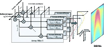
The generic correlation channel based on the multiply and accumulate (MAC) approach (Kaplan and Hegarty, Reference Kaplan and Hegarty2006) is just designed for performing correlation at a single “point” (delay/Doppler peak) and cannot compute the DDMs in parallel. FFT (Fast Fourier Transforms) based correlation method (Van Nee and Coenen, Reference Van NeE and Coenen1991) provides the correlation value for all the possible code phases in parallel, but it would lead to a waste of hardware resources. In order to balance speed and hardware resources, the correlation channel for reflected signal is designed as parallel-correlator-array architecture. As shown in Figure 3, the correlation channel is a correlator array comprising N Doppler delay-dimensional slices. In each slice, the incoming reflected signal s R(n) is down-converted by a local complex carrier associated to a given Doppler bin and multiplied with the local generated C/A codes group (LoCG) corresponding to N delay delay coordinates and the resulting complex signal pairs (I+jQ) are then accumulated to obtain the delay-dimensional waveform. The waveforms output by different slices can be further synthesized as a complete DDM.
Architecture and signal processing scheme of the correlation channel for reflected signal.

3.2. Carrier and Code Generation
The generation of carrier and C/A code for reflected signal correlation channel is based on the following considerations:
• to accommodate the open-loop processing mode of reflected signals as explained in section 3.4;
• to improve the resolutions of both code delay (Δτ) and Doppler offset (Δf D).
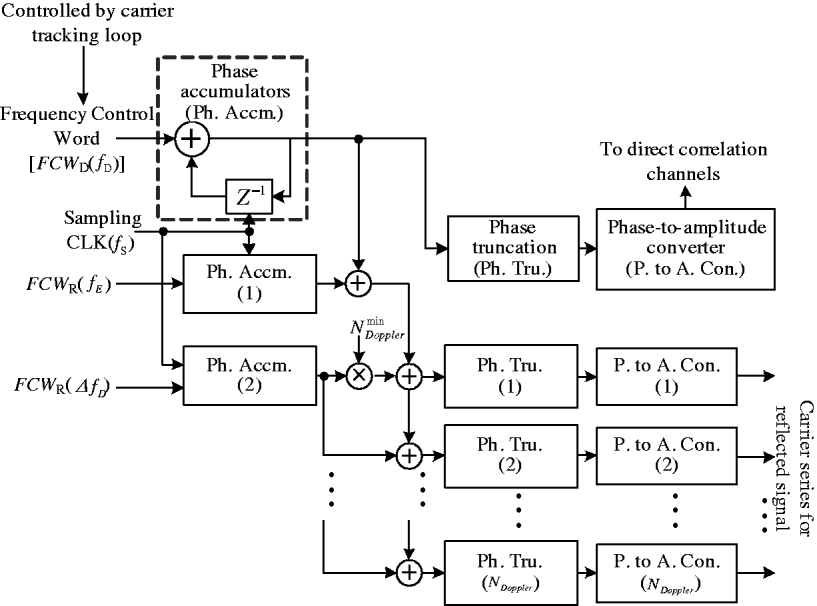
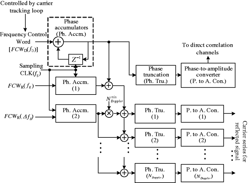
As shown in Figure 4, the generation of carrier series for reflected signal is based on numerically-controlled oscillators (NCO). The carrier phases of direct signals are adopted as reference to compensate the Doppler shift of direct signal. The mean Doppler shift between the direct and reflected signal and Doppler resolution can be set through FCW R(fE) and FCW R(ΔfD).
Carrier series generation scheme with different Doppler.
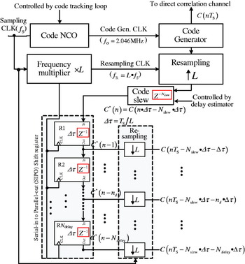
The C/A codes with different time delays are generated through a cascaded delay line which simultaneously provides delayed replicas of the original C/A code synchronous with the direct signal. To achieve a high resolution, a multi-rate processing method is adopted. As shown in Figure 5, the original C/A code sequence C(nT S) is re-sampled by RCLK at L times the rate of sampling clock (L·f S) and slewed to generate an additional time delay. The resulting sequence C*(n) is then delayed through an N delay-lag (each lag corresponds to a delay of one RCLK cycle) Serial-in to Parallel-out (SIPO) shift register. The output sequences of each shift register are re-sampled by the sampling CLK to provide the N delay delayed replicas with a resolution of Δτ expressed as:

and the resolution can be set through L.
C/A code series generation with different time delays.

3.3. DDM Parameter in Practical Implementation
DDM parameters including:
• the DDM size in both delay and Doppler domains (N delay×Ndoppler),
• the resolution of code delay (Δτ) and Doppler offset (Δf D) and
• the number of correlation channels (N Channel) for different satellites processed simultaneously,
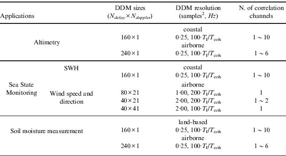
are limited by the logic resources of the FPGA chip. Moreover, the requirements of these parameters are dependent on the geometry of the signal reflection and eventually on the characteristics of the reflecting surface. For different application fields, the DDM parameters are dynamically configurable in GRrSv.2. Some typical configurations are listed in Table 1 and those parameters can also be configured as other available values.
Typical configurations of DDM parameters1.
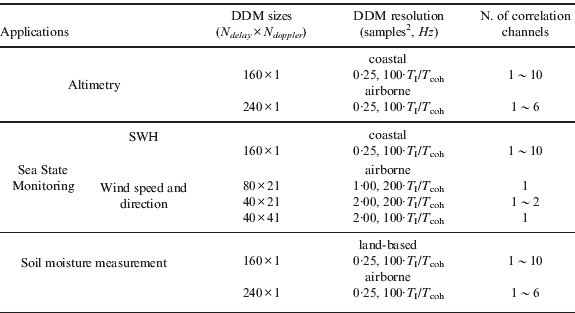
1 DDM size and number of correlation channels are limited by the hardware resources and should satisfy that N delay×N doppler×N Channel<1700.
2 1 sample =0·05 chip.
3.4. Delay and Doppler Synchronisation
During the computing of DDMs, the delay and Doppler values ( ) of the DDM peak should be estimated continuously to properly align the reflected signal correlation window.
3.4.1. Doppler Synchronisation
According to Equation (3), the Doppler shift of reflected signal can be expressed as:

The temporal derivative of f D is tracked by the carrier tracking loop of the direct signal and f E is estimated by Equation (10) every second:

where  and
 are the velocity vector of the transmitter and receiver,
 and
 are the incidence and reflecting direction unitary vector and
 is the unitary vector of direction between the transmitter and receiver. Both velocity and direction vectors are computed through the navigation solutions by the DSP processor.
3.4.2. Delay Synchronisation
The range delay of reflected signal ρ R can be expressed as:

where c is the speed of light in vacuum, ρ D represents the path delay of direct signal, and Δρ E is the excess path delay between reflected and direct signals.
The temporal derivative of the delay ρ D can be tracked with a precision of 10–2 chip during the processing of the direct signal and the additional delay Δρ E is determined from the geometry by the relation

where h R represents the height of the receiver above the reference ellipsoid, h U represents the height undulation between the reflecting surface and the reference ellipsoid level, and θ represents the elevation of the GPS satellite. Both h R and θ are provided through the navigation solutions and the unknown deviation h U is eliminated by the following process:
(1) Estimate the coarse delay difference Δρ ECoarse by
and slew the LoCG by a code phase corresponding to Δρ ECoarse.(2) Calculate the envelope of the delay-dimensional waveform E(n d) with zero Doppler offset in the current delay-Doppler window.
(3) Detect the maximum of E(n d). If the maximum is below a threshold setting, slew the LoCG by a code phase step of N delay·Δτ and go back to step (3), else go to step (4).
(4) Finely slew the LoCG by the step of Δτ to make the delay peak at a given position of the delay window.
(5) Adjust the code phase of each 10 millisecond to track the delay-Doppler peak to the fix position in the delay-Doppler window.
 and slew the LoCG by a code phase corresponding to Δρ ECoarse.
4. EXPERIMENTS AND RESULTS
4.1. Aircraft Experiment for Ocean Remote Sensing
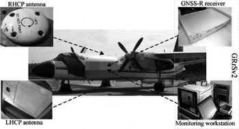
From February to March 2009, aircraft-based experiments for ocean remote sensing were undertaken at ∼5500 m above the mean sea level and ∼107 m/s speed over the sea areas of the eastern Hainan. A YUN-7 aircraft was used in our campaigns, and system installation condition is shown in Figure 6.
System installation during flight campaigns: the RHCP antenna was mounted on the top of the Y-7 to collect the direct signals, and the LHCP antenna was mounted on the belly of the Y-7 to collect the sea reflected signals.

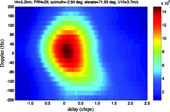
The purpose of the flights was to evaluate the system's availability for sea surface wind measurement through the real-time computed DDMs as shown in Figure 7. Moreover, in-situ wind vectors from QuikSCAT and Bo'ao ocean station were collected as reference during the data analysis.
Power of the sample DDM (40×41) over sea on 11 Feb. 2009 from GPS PRN 28 at 71·93 degrees elevation after 10 ms coherent and 100 ms incoherent integration. In-situ QuikSCAT data indicated that the ocean wind speed was 3·7 m/s. These observations were obtained by configuring the system with delay of −1·5 to 2·5 chip in 0·1 chip resolution and Doppler of −200 to 200 Hz in a 10 Hz resolution.

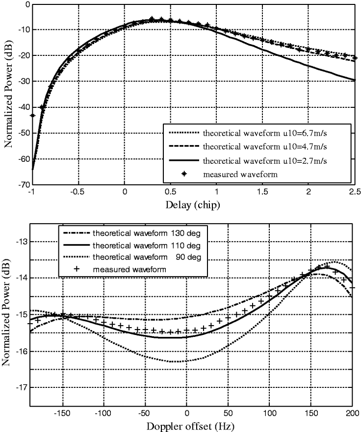
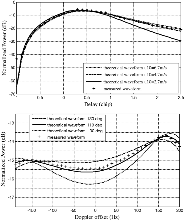
Figure 8 illustrates the comparison between the measured and theoretical waveforms. The measured waveforms are obtained from the DDMs of GPS PRN 15 on 21 February 2009 after 10 ms coherent and 100 ms incoherent integration and the theoretical waveforms are generated using the Z-V scattering model (Zavorotny and Voronovich, Reference Zavorotny and Voronovich2000) with inputs from the Elfouhaily wave spectrum (Elfouhaily et al., Reference Elfouhaily, Chapron, Katsaros and Vandemark1997) according to the in-situ ocean station data. The great concordance between the measured and theoretical waveforms shows that the DDMs computed by the system are valid for sea surface wind measurement.
Comparison between theoretical and measured waveforms. (Top) Normalized power vs. code delay (the power is obtained by summing all the delay domain waveforms of a DDM from different Doppler offsets). (Bottom) Normalized power vs. Doppler offset (the power is obtained directly from a DDM at the constant code delay of 2·5 chip). In-situ ocean station data indicated that the ocean wind speed was 4·7 m/s and the ocean wind direction was 110°.
4.2. Coastal Experiment for Sea State Determination
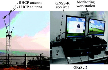
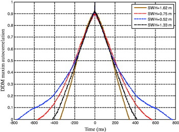
Coastal experiments have been performed since 22 November 2009 at Maoming ocean meteorological station, Guangdong. The system installation condition is shown in Figure 9. During the experiments, only delay domain waveforms were computed and output directly without coherent or incoherent integration. The maximum of those waveforms are selected as representative point for further analysis. During the experiments, two typical sequences of those representative points (each sequence contains 30 000 complex points, namely 30 s) corresponding to different sea states are acquired with the same reflecting geometry. The autocorrelation of these sequences is computed and shown in Figure 10, which corresponds with the fact that the coherence time of the reflected signal varies with the significant wave height (SWH). It shows that the system can be used by the applications that require phase information.
System installation during the coastal experiments: the RHCP and LHCP antennas were settled on the top of the station, with the RHCP antenna zenith-oriented and the LHCP antenna pointing to the sea surface. The maximum distance between the antenna and sea surface is about 21 m.

Autocorrelation of the DDM maximum of two sequences corresponding to different sea states of SWH=1·62 m, 0·75 m, 0·52 m and 1·33 m. The four sequences were obtained from the DDMs of GPS PRN 28 on 18 February, 4 June, 20 August and 26 October 2010 at the same elevation of ∼21°.

4.3. Ground-based Experiments for Soil Moisture
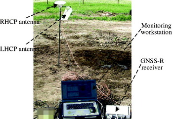
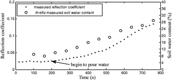
Ground-based experiments were performed to demonstrate the availability of the system in remote sensing of land areas in May, 2009. As shown in Figure 11, the RHCP and LHCP antennas were mounted on a shelf with the RHCP antenna oriented toward zenith and the LHCP antenna facing a bare soil field. After collecting data for a while, water is poured the field every 60 s. The reflection coefficient which is defined as the power ratio of DDM peak point and the directed signal tracking point is shown in Figure 12, together with the in-situ measured soil water content. It can be seen that the power of the DDM peak is sensitive to the soil moisture and that the system can be used in soil moisture measurement.
System installation during the ground-based experiments.

Comparison between reflection coefficient and in-situ measured water content. The observations were obtained from GPS PRN 14 on 23 May 2009.

5. CONCLUSIONS AND DISCUSSION
A technical description of the GRrSv.2 has been presented in this paper, including the system architecture and reflected signal processing issues. The designed system can compute complex DDMs in real-time with high accuracy and stability by means of advanced digital design techniques and can be used in many different GNSS-R application fields. The system has already been tested in both aircraft- and ground-based experiments over sea and land with very promising results. Further research activities that are being undertaken include:
• the analysis of experimental data to study the retrieval methods on the related applications;
• performing more experiments on other GNSS-R applications such as ocean altimetry, sea ice sensing, ocean salinity measurement and bistatic synthetic aperture imaging and making further improvements of the system according to the experiment results;
• studying the key technologies of space-based GNSS-R signal receiving and processing methods, such as antenna array with digital beam-forming, high-precision reflecting geometry computing and high dynamic reflected signal synchronisation.