Introduction
Choice of appropriate temporal scale and resolution of sampling is at the heart of any hypothesis testing because it has a decisive effect on interpretation of the results of a field study (Green, Reference Green1979; Baker & Wolff, Reference Baker and Wolff1987; Livingston, Reference Livingston1987; Baretta & Malschaert, Reference Baretta and Malschaert1988). There exists little guidance on sampling scales for estuaries because of extreme variability of the main variables such as salinity, temperature, chl a which change with every tide and with seasonal cycles (Weglenska, Reference Weglenska1976; Green, Reference Green1979; Baker & Wolff, Reference Baker and Wolff1987; Livingston, Reference Livingston1987; Baretta & Malschaert, Reference Baretta and Malschaert1988; David et al., Reference David, Sautour, Chardy and Leconte2005). Temporal scale and resolution of sampling must take into account the environmental and ecological complexities of estuaries (Weglenska, Reference Weglenska1976; Millard & Lettenmaier, Reference Millard and Lettenmaier1986; Baker & Wolff, Reference Baker and Wolff1987; Baretta & Malschaert, Reference Baretta and Malschaert1988). For most estuaries of developing/poor nations, sampling efforts are curtailed by lack of sustained funding and infrastructure, and inadequate logistics for long-term studies. These factors negatively affect the process of hypothesis testing; for such reasons, many estuarine studies provide ecological perspectives from limited field surveys (Baker & Wolff, Reference Baker and Wolff1987; Baretta & Malschaert, Reference Baretta and Malschaert1988; Devreker et al., Reference Devreker, Souissi, Molinero, Beyrend-Dur, Gomez and Forget-Leray2010).
Copepods often dominate estuarine zooplankton assemblages (Baretta & Malschaert, Reference Baretta and Malschaert1988; David et al., Reference David, Sautour, Chardy and Leconte2005; Costa et al., Reference Costa, Leite and Pereira2009; Paul et al., Reference Paul, Wooldridge and Perissinotto2016). Many long-term estuarine copepod studies have examined their density changes in relation to variation of salinity, temperature and chl a. Depending on the temporal scales of study, copepod density, taxonomic richness and dominance change in specific season(s) because seasonal changes bring changes in temperature which in turn bring variability in primary production (Livingston, Reference Livingston1987; Taylor, Reference Taylor1987, Reference Taylor1993; Baretta & Malschaert, Reference Baretta and Malschaert1988; Cloern, Reference Cloern1999; Warwick et al., Reference Warwick, Ashman, Brown, Clarke, Dowell, Hart, Lewis, Shillabeer, Somerfield and Tapp2002; Hoffmeyer, Reference Hoffmeyer2004; David et al., Reference David, Sautour, Chardy and Leconte2005; Devreker et al., Reference Devreker, Souissi, Molinero and Nkubito2008; Jang et al., Reference Jang, Shin, Hyun, Lee and Choi2013). Temporal changes in copepod densities are suggested as ecological indicators of salinity and temperature stress for large open estuaries (Paul et al., Reference Paul, Wooldridge and Perissinotto2016), so could be used for long-term monitoring of environmental and or anthropogenic stress of estuaries. Generally, a short-term high-resolution (STHR) sampling protocol better captures the time variability of copepod densities compared to a medium-term low-resolution (MTLR) sampling protocol because shorter scales capture more noise within a data set. Despite this, consensus on the temporal scale and resolution of sampling for providing consistent information on the temporal variability of an estuarine copepod population density has yet to be reached.
Rio de la Plata (RdlP) is an estuary of South America which is bordered by Uruguay and Argentina (Acha et al., Reference Acha, Mianzan, Guerrero, Carreto, Giberto, Montoya and Carignan2008). Temporal changes of its salinity and temperature bring variability in chl a production which sustains high plankton densities (Calliari et al., Reference Calliari, Gómez and Gómez2005; Carreto et al., Reference Carreto, Montoya, Akselman, Carignan, Silva and Colleoni2008). Zooplankton assemblages of RdlP are often dominated by copepods of various size classes (Berasategui et al., Reference Berasategui, Marque, Gómez-Erache, Ramírez, Mianzan and Acha2006). Acartia tonsa is a copepod species that is perennial in nature and dominates (in terms of abundance) the copepod community of RdlP (Paul et al., Reference Paul, Castiglioni, Cervetto and Calliari2017). Paracalanus parvus is a seasonal copepod species which remains within a typical copepod assemblage but is generally associated with more saline waters (Berasategui et al., Reference Berasategui, Marque, Gómez-Erache, Ramírez, Mianzan and Acha2006). For the present investigation A. tonsa and P. parvus were respectively used as examples of perennial and seasonal copepods within the brackish zone of RdlP. We hypothesized that a short-term high-resolution (STHR) sampling protocol would better capture the time variability of copepod population densities in relation to salinity, temperature and chl a changes than a medium-term low-resolution (MTLR) sampling protocol could. This study may provide a better understanding of sampling frequency of an estuarine copepod for studying its population density.
Materials and methods
Sample collection
Sampling (all of which was conducted at low tide) was intended for studying seasonal changes in copepod population densities, so samples were collected in every month of 2003 (except December). At least in one month of each season samples were taken on a weekly basis except in winter when the samples were collected at fortnightly intervals because of economic resource limitations. Samples were collected at Playa del Buceo (a coastal site off Montevideo) in waters about 1.5 m deep just after sunset (Figure 1). Sub-surface (~1.5 m water depth) tows were made using a 35 cm mouth plankton net fitted with 180 µm pore size mesh. Volume of water sampled was about 19 m3 on each tow. Samples were preserved in 4% formalin solution (final concentration). Copepods were identified and counted under a low magnification microscope. Abundance of each species was expressed as individuals per cubic metre (ind. m−3).
Sample collection site in Rio de la Plata off Montevideo, Uruguay.

On every sampling occasion water temperature and salinity were measured (from ~1.5 m water depth) using a multi-probe sensor (Horiba U 10, Japan) and water samples were collected for chl a analysis whenever copepods were collected. 50 ml subsamples were filtered through GF/F filters, and pigments extracted in 96% ethanol in the dark at 4°C for 24 h. The fluorescence of the resulting extract was read before and after acidification (HCl 1.2 N) in a Turner 111 Fluorometer calibrated against standard chl a extract. These data were collected in order to evaluate if the temporal variations of temperature, salinity and chl a had significantly affected the population densities of copepods A. tonsa and P. parvus.
Dataset arrangement
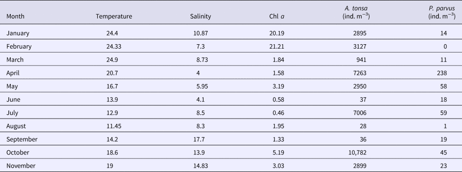
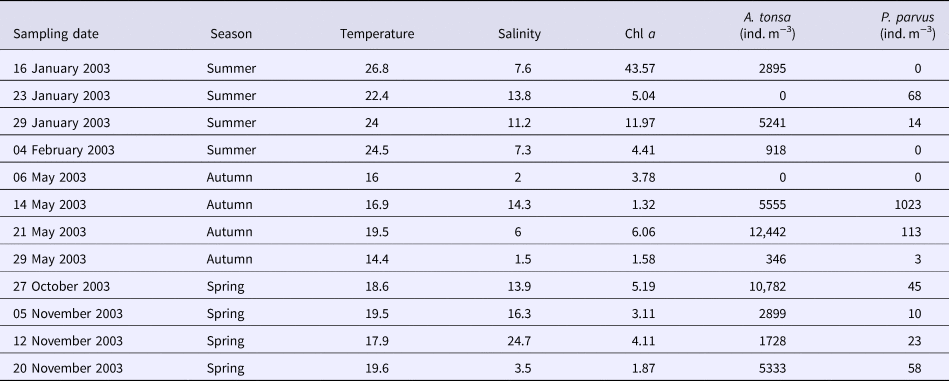
The study aimed to identify the scale and resolution of sampling effort that provides the maximum information on variability of copepod population densities in relation to temporal physicochemical changes in their habitat. To address these, two separate data sets were analysed. (1) ‘Yearly Dataset (YD)’ (see Table 1) was essentially the monthly data (one measurement/month) and included salinity, temperature, chl a, and densities of A. tonsa and P. parvus. YD was assumed as an example of a MTLR dataset. (2) ‘Seasonal Weekly Datasets (SWD)’ was essentially the data of four consecutive weeks (one measurement/week) of sampling effort and had information on salinity, temperature, chl a, and densities of the copepods A. tonsa and P. parvus (see Table 2). SWD was assumed as an example of a STHR dataset. Analysis of SWD was run separately for each season (because it is essentially a seasonal sampling effort) except for winter because of very limited economic resources available for sampling so the resultant data set was too small to include in the statistical analysis.
Yearly Dataset (YD) that consists of monthly data of copepod Acartia tonsa and Paracalanus parvus densities (ind. m−3) along with salinity, temperature, and chl a data collected from Rio de la Plata off Montevideo, Uruguay, between January and November 2003

Seasonal Weekly Datasets (SWD) that consist of four consecutive inter-week data of copepod Acartia tonsa and Paracalanus parvus densities (ind. m−3) along with salinity, temperature, and chl a data of Rio de la Plata off Montevideo, Uruguay, in summer, autumn and spring of 2003

Sampling in winter was limited due to economic constraints.
Statistical analysis
The Shapiro–Wilk normality test found salinity (W = 0.93; P = 0.16), temperature (W = 0.95; P = 0.44) were normally distributed but chl a (W = 0.49, P <0.001) was not. Seasonal variations of physicochemical factors were checked either by ANOVA or by Kruskal–Wallis (for non-Gaussian data) followed by Tukey's or Nemenyi post-hoc test (if required). Copepod densities followed a quasi-Poisson distribution so the generalized linear models of quasi-Poisson distribution family were built to evaluate if there were significant temporal changes in the densities of copepods A. tonsa and P. parvus due to time variability of salinity, temperature and chl a. ‘glmmPQL’ function of the ‘MASS’ package of CRAN-R3.4.1 for x86_64-apple-darwin15.6.0 (64-bit) was used for this purpose. Confidence intervals were set at 95% and respective W, t, P, df were reported.
Results
Analysis of the YD
Mean temperature was 18.28 ± 4.8°C (range 11.45–24.9°C); temperature fluctuated between seasons (ANOVA: df = 3, F = 19.5, P = 0.0008) (Table 1). Mean salinity was 9.47 ± 4.43 which fluctuated between seasons (ANOVA: df = 3, F = 13.75, P = 0.002) especially in autumn and winter when the salinity dropped considerably (4–4.1) but increased in spring (17.7) (Table 1). Chlorophyll a (median) was 1.95 µg l−1, and was highest in summer (21.21) and lowest in winter (0.46) (Table 1).
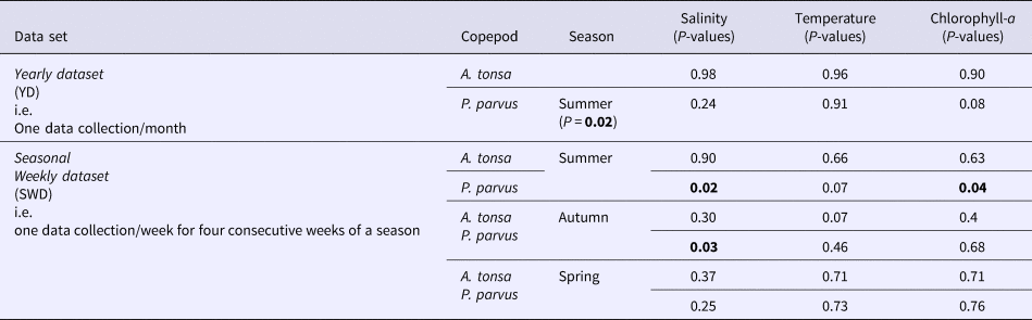
Density of the A. tonsa population did not vary significantly between seasons but was relatively lower in June and August and the maximum density was recorded in October (Table 1). Density of A. tonsa was not much affected by temporal variability of salinity, temperature and chl a (Tables 1 and 3). Paracalanus parvus density was significantly lower in summer (df = 7, t = −2.93, P = 0.02), andpeaked in autumn (Tables 1 and 3), but was not significantly influenced by the temporal variability of temperature, salinity and chl a (Tables 1 and 3).
Comparison of different temporal scales and resolutions of variability of Acartia tonsa and Paracalanus parvus densities (ind. m−3) in relation to salinity, temperature and chl a. P values in bold are statistically significant (P < 0.05)

Analysis of the SWD
In summer the mean temperature, salinity and chl a (median) were 24.42 ± 1.81°C, 9.97 ± 3.1 and 8.50 µg l−1, respectively (Table 2). Acartia tonsa density ranged from 0 to 5241 ind. m−3 and peaked in late January (Table 2) but the density was not significantly affected by time variability (inter-week) of temperature, salinity and chl a (Table 3). Paracalanus parvus density ranged from 0 to 68 ind. m−3 and the highest density was in mid-January (Table 2). Density of P. parvus population did increase in high salinity (df = 2, t = 7.2, P = 0.02) but the higher availability of chl a limited their density (df = 2, t = −4.68, P = 0.04) (Table 3). In autumn the mean temperature and salinity were 16.7 ± 2.13°C and 5.95 ± 5.91 respectively. Chlorophyll a (median 2.68 µg l−1) ranged between 1.32 and 6.06 µg l−1 (Table 2). Acartia tonsa density ranged from 0 to 12,444 ind. m−3 and the highest density was recorded in mid-autumn (Table 2), but density was not affected by time variability (inter-week) of temperature, salinity and chl a (Table 3). Paracalanus parvus density ranged from 0 to 1023 ind. m−3 with the highest density recorded in mid-autumn (Table 2). Density of P. parvus increased with the salinity (df = 2, t = 5.05, P = 0.037), but chl a had no such effect on its density (Table 3).
In spring the mean temperature was 18.9 ± 0.8°C; salinity was 14.6 ± 8.72; chl a (median) was 3.61 µg l−1 and ranged between 1.87 and 5.19 µg l−1 (Table 2). Acartia tonsa density ranged from 1728 to 10,782 ind. m−3 with the highest density recorded in late October, and P. parvus density ranged from 10 to 58 ind. m−3 with the highest density recorded in late November (Table 2). Densities of A. tonsa and P. parvus were not much affected by the temporal changes (inter-week) of temperatures, salinity and chl a (Table 3).
Discussion
Given that shorter scales always capture more noise within a dataset, we predicted that STHR sampling (exemplified through SWD analysis) would capture more variability of temporal changes in copepod densities in relation to physicochemical changes of RdlP than a MTLR sampling (exemplified through YD analysis) could do. STHR sampling found P. parvus density to increase with salinity in summer and autumn but to decrease with high concentration of chl a in summer; MTLR sampling failed to show such relationships of population density changes of P. parvus, which supports the prediction. Analysis of YD found that the A. tonsa density was neither significantly affected by seasonal cycles nor by temporal variability of salinity, temperature and chl a. Similarly, analysis of SWD found that the variability of A. tonsa population density in association with inter-week changes of salinity, temperature and chl a was not significant. Thus, STHR and MTLR sampling protocols ended up providing similar information on the variability of A. tonsa population densities in association with temporal changes of the physicochemical characteristics of RdlP; such results contradict the hypothesis.
Acartia tonsa is a typical estuarine and coastal marine copepod well adapted to the fluctuations of salinity, temperature and chl a gradients of its habitats (Baretta & Malschaert, Reference Baretta and Malschaert1988; Mauchline, Reference Mauchline1998; Cervetto et al., Reference Cervetto, Gaudy and Pagano1999; Castro-Longoría, Reference Castro-Longoría2003; Hubareva et al., Reference Hubareva, Svetlichny, Kideys and Isinibilir2008). This could be a reason that the species is found in tropical to temperate coastal-marine waters (González, Reference González1974; Cervetto et al., Reference Cervetto, Gaudy and Pagano1999; Paul et al., Reference Paul, Castiglioni, Cervetto and Calliari2017). In the RdlP, irrespective of season, A. tonsa numerically dominates zooplankton assemblages compared with other meso-zooplankton (Berasategui et al., Reference Berasategui, Marque, Gómez-Erache, Ramírez, Mianzan and Acha2006; Paul et al., Reference Paul, Castiglioni, Cervetto and Calliari2017). In the Bahia Blanca estuary of temperate Argentina, the temperature cycle is the main driver of species succession of A. tonsa dominance (Hoffmeyer, Reference Hoffmeyer2004). In the Patos Lagoon of Brazil during the colder season higher salinities favour dominance of A. tonsa (Montú, Reference Montú1980; Montú et al., Reference Montú, Duarte, Gloeden, Seeliger, Odebrecht and Castello1997). In the subtropical estuaries of USA, A. tonsa density peaks in summer, especially towards the more saline zones (Lawrence et al., Reference Lawrence, Valiela and Tomasky2004). The sampling location Playa del Buceo is characterized by an oligohaline to mesohaline salinity profile and moderate temperature variability (Paul et al., Reference Paul, Castiglioni, Cervetto and Calliari2017), and is not a habitat characterized by high phytoplankton biomass throughout the seasons. Considering such conditions in RdlP, the perennial presence and dominance of A. tonsa are not that surprising (Berasategui et al., Reference Berasategui, Marque, Gómez-Erache, Ramírez, Mianzan and Acha2006; Paul et al., Reference Paul, Castiglioni, Cervetto and Calliari2017). We suggest that in such a case, extrapolation of the temporal scale and resolution of sampling A. tonsa may not lose much information on variability of population densities in association with physicochemical parameters. Long-term monitoring of estuaries is often discouraged by institutions because of resource constraints such as lack of sustained funding, skilled manpower, infrastructural facilities etc., so for perennial copepods such as A. tonsa a STHR strategy can be followed.
Paracalanus parvus is a neritic species distributed along the margins of the South-west Atlantic (Mauchline, Reference Mauchline1998). In the San Francisco Bay of the USA it is distributed towards the seaward boundary (Ambler et al., Reference Ambler, Cloern and Hutchinson1985). In the present study, analysis of SWD found a significant positive association of salinity and P. parvus population density which clearly reflects their preference for salty conditions. A 10-year weekly/bi-weekly survey in the sub-tropical Korean waters showed that P. parvus biomass closely followed a seasonal pattern of abundance with high densities when the water temperature exceeded 20°C (Jang et al., Reference Jang, Shin, Hyun, Lee and Choi2013). In RdlP, P. parvus densities increased in late summer–autumn when the temperature ranged between 16 and 26°C, which agrees with the Korean study. Analysis of SWD (not of YD) indicated that in summer the population density of P. parvus was limited by the presence of high chl a in RdlP. Such a result is somewhat paradoxical considering P. parvus is an herbivorous copepod (Morales et al., Reference Morales, Bedo, Harris and Tranter1991). It could be the case that the observed negative correlation of P. parvus density and chl a was due to the effect of a third variable associated with both, for example salinity, and thus would not represent a causal or mechanistic relationship. In future more frequent sampling (for example daily) is advised to better understand how the changes in chl a concentration in RdlP affects P. parvus density. Since P. parvus is mostly present in the warmer months (e.g. autumn) a STHR sampling is advised during that time to gain detailed insights of the population characteristics (e.g. density change, changes in age class) of P. parvus and also its relationships with the physicochemical characteristics of RdlP.
The results demonstrated that STHR and MTLR sampling for studying the variability of copepod densities in relation to physicochemical changes of RdlP yielded similar ecological information for A. tonsa. A detailed insight of the variability of population density of P. parvus was achieved only through the STHR sampling. Such contrasting outcomes highlight the issue of what amounts to appropriate scaling to address spatial and or temporal questions relating to estuaries (Green, Reference Green1979; Baker & Wolff, Reference Baker and Wolff1987; Livingston, Reference Livingston1987; Baretta & Malschaert, Reference Baretta and Malschaert1988). Livingston (Reference Livingston1987) while extrapolating weekly to monthly sampling results of a decade of study of the Apalachicola Bay system suggested that temperature can be adequately represented by monthly data but salinity cannot because of its high variability. In the present study the MTLR sampling failed to find statistically significant effects of salinity and chl a changes on the variation in P. parvus density which the STHR sampling successfully found. Thus, to understand the relationships of temporal variability of salinity and chl a with densities of seasonal copepods like P. parvus, STHR sampling is possibly a recommended way because of the higher variability of salinity and Chl-a in large open estuaries. The present study suggests that for a highly abundant, perennial and highly tolerant copepod such as A. tonsa its association with temperature, salinity and chl a changes in estuaries could be adequately studied by either the MTLR or STHR approaches depending on the availability of resources (e.g. economic, manpower, logistics etc.). Understanding the impact of longer-term processes linked to climatic change and low frequency oscillations (for example, the ENSO cycles) requires observations at scales matching the processes of interest. However, due to limited institutional resources (i.e. economic and infrastructural) any long-term data of zooplankton or copepods may remain unavailable for some of the most economically important estuaries because they are in poor and developing countries (e.g. the RdlP, Amazon River, Nile River, Ganges River, Mekong River). Copepod sampling can provide an ecological indication of abiotic/anthropogenic stressors and food web health quality of a given coastal zone which may be important for regional fisheries (David et al., Reference David, Sautour, Chardy and Leconte2005; Paul et al., Reference Paul, Wooldridge and Perissinotto2016). Thus in future, copepod sampling within a very limited budget directed to explore a specific hypothesis of species-specific responses to water quality or environmental variability is more feasible than long-term monitoring programmes (Livingston, Reference Livingston1987; Baretta & Malschaert, Reference Baretta and Malschaert1988; David et al., Reference David, Sautour, Chardy and Leconte2005; Devreker et al., Reference Devreker, Souissi, Molinero, Beyrend-Dur, Gomez and Forget-Leray2010). In such cases, short-term approaches as discussed here could provide complementary information for the interpretation of results from a long-term observation.
Acknowledgements
The first author thanks the Department of Science & Technology of India (in particular DST-INSPIRE Faculty Award for his fellowship) and Department of Zoology of University of Calcutta for the facilities provided for preparation of this manuscript. Sección Oceanografía, Facultad de Ciencias-Universidad de la República, Uruguay, is thanked for supporting the research costs and facilities provided therein.
Financial support
DST-INSPIRE Faculty Award (DST/INSPIRE/04/2016/000036) of Department of Science & Technology of India is hereby acknowledged by the first author for his fellowships. The second author acknowledges the National Agency of Research and Innovation ANII, Uruguay for financial support.