



1. Introduction
Kolmogorov (Reference Kolmogorov1941a
,
Reference Kolmogorovb
) proposed two hypotheses to describe and predict small-scale turbulent motions, which require very large Reynolds numbers. The first hypothesis states that, for locally homogeneous and isotropic turbulence, there exists a universal small-scale equilibrium range in which the turbulent statistics are determined solely by the mean energy dissipation rate
 $\overline {\varepsilon }$
(the overbar denotes a temporal or spatial average) and the kinematic viscosity
 $\nu$
. Based on this hypothesis, Kolmogorov used dimensional analysis to derive the velocity scale
 $u_K = (\overline {\varepsilon } \nu )^{1/4}$
and the length scale
 $\eta = (\nu ^3/\overline {\varepsilon })^{1/4}$
. The second hypothesis further states that an inertial subrange exists at scales much larger than
 $\eta$
but much smaller than the integral length scale associated with the energy-containing large-scale motions. Within this subrange, the statistics are governed exclusively by
 $\overline {\varepsilon }$
, and viscous effects are negligible. Consequently, dimensional analysis yields the well-known
 $-5/3$
power law
 \begin{align} E(\kappa ) = C_{K} \overline {\varepsilon }^{2/3} \kappa ^{-5/3}, \end{align}
where
 $E(\kappa )$
is the three-dimensional energy spectrum,
 $C_{K}$
is the Kolmogorov constant and
 $\kappa$
is the wavenumber. The
 $-5/3$
scaling has been widely observed in locally homogeneous and isotropic turbulence at very large Reynolds numbers and has become a cornerstone of turbulence research (e.g. Grant et al. Reference Grant, Stewart and Moilliet1962; Saddoughi & Veeravalli Reference Saddoughi and Veeravalli1994; Sreenivasan Reference Sreenivasan1995; Yeung & Zhou Reference Yeung and Zhou1997; Gotoh et al. Reference Gotoh, Fukayama and Nakano2002; Tsuji Reference Tsuji2004; Ni & Xia Reference Ni and Xia2013; Ishihara et al. Reference Ishihara, Kaneda, Morishita, Yokokawa and Uno2020; Meldi et al. Reference Meldi, Djenidi and Antonia2021).
However, at relatively low Reynolds numbers, numerous studies (Parnaudeau et al. Reference Parnaudeau, Carlier, Heitz and Lamballais2008; Wissink & Rodi Reference Wissink and Rodi2008; Gomes et al. 2014, Reference Gomes, Ganapathisubramani and Vassilicos2015; Laizet et al. Reference Laizet, Nedić and Vassilicos2015; Paul et al. Reference Paul, Papadakis and Vassilicos2017, Reference Paul, Papadakis and Vassilicos2018; Portela et al. 2017, Reference Portela, Papadakis and Vassilicos2020; Zhou et al. 2018, 2019, Reference Zhou, Zhou, Yiu and Chua2020, Reference Zhou, Nagata and Ito2023; Yasuda et al. Reference Yasuda, Goto and Vassilicos2020; Ortiz et al. Reference Ortiz, Nidhan and Sarkar2021) have reported that the energy spectra can also exhibit an approximate
 $-5/3$
scaling over a limited range. In particular, this scaling can persist even in the near wake, where large-scale coherent structures are present. For instance, in the near field (
 $x/d = 6$
) of a circular cylinder at
 $ \textit{Re}_{d} = 3300$
, Wissink & Rodi (Reference Wissink and Rodi2008) observed a weak signature of the
 $-5/3$
scaling in the frequency spectrum
 $\phi _{u}(f)$
, where
 $f$
denotes frequency. In this paper, the one-dimensional streamwise, lateral and spanwise energy spectra are denoted by
 $\phi _{u}$
,
 $\phi _{v}$
and
 $\phi _{w}$
, respectively. Here,
 $u_i$
is the fluctuating velocity component in the
 $x_i$
direction and
 $u_1$
,
 $u_2$
, and
 $u_3$
will be used interchangeably with
 $u$
,
 $v$
,
 $w$
; similarly for
 $x_1$
,
 $x_2$
,
 $x_3$
and
 $x$
,
 $y$
,
 $z$
. The Reynolds number is defined as
 $ \textit{Re}_{d}=U_{\infty }d/\nu$
, based on the free-stream velocity
 $U_{\infty }$
and the cylinder diameter
 $d$
(or the side width of a square cylinder). Similarly, in the near wake (
 $x/d = 1-8$
) of a square cylinder at
 $ \textit{Re}_{d} = 3900$
, Portela et al. (Reference Portela, Papadakis and Vassilicos2017, Reference Portela, Papadakis and Vassilicos2020) reported an approximate
 $-5/3$
scaling in the centreline distributions of
 $\phi _{u}(f)$
,
 $\phi _{v}(f)$
and
 $\phi _{w}(f)$
, despite the strong inhomogeneity and anisotropy of the flow. Furthermore, using the Kármán–Howarth–Monin–Hill equation, they showed that this scaling coexists with an inverse energy cascade. In the same flow configuration at
 $ \textit{Re}_{d} = 2500$
, Zhou et al. (Reference Zhou, Nagata and Ito2023) identified an approximate
 $-5/3$
scaling in the
 $\phi _{u}(\kappa _1)$
distributions at
 $x/d = 6$
and
 $26$
, where
 $\kappa _1$
is the streamwise wavenumber. For two side-by-side square cylinders at the same Reynolds number, Zhou et al. (Reference Zhou, Nagata, Sakai and Watanabe2019, Reference Zhou, Nagata, Sakai, Watanabe, Ito and Hayase2020) observed an approximate
 $-5/3$
scaling in the
 $\phi _{u}(f)$
distribution over a broad frequency range at
 $x/d = 6$
, where the turbulence is still developing and strongly intermittent. They found that this power-law behaviour is closely associated with large-scale vortex shedding and so-called extreme events, characterised by abrupt jumps in velocity fluctuations and strongly non-Gaussian statistics with high flatness. A similar interpretation was proposed for the near field of grid-generated turbulence (Gomes et al. Reference Gomes, Ganapathisubramani and Vassilicos2015), where the scaling originates from regions of highly intermittent, non-Gaussian turbulent fluctuating velocities. They argued that the scaling results from interactions among clusters of elongated vortices and the intermittent nature of their appearance. In addition, Yasuda et al. (Reference Yasuda, Goto and Vassilicos2020) identified a
 $-5/3$
scaling in the shear-layer region of near-field grid-generated turbulence and suggested that it forms through cooperative interactions between large-scale structures from vortex shedding and small-scale structures from shear-layer instabilities.
The above studies have provided useful insights into the
 $-5/3$
scaling in wakes. Nevertheless, a comprehensive understanding of this phenomenon in bluff body wakes is still lacking. In particular, several fundamental questions remain. How does the
 $-5/3$
scaling depend on velocity components, spatial location, geometry of the bluff body and Reynolds number? How does the
 $-5/3$
scaling observed in the wake differ from that in the inertial subrange of homogeneous and isotropic turbulence? To address these questions, we conduct a detailed examination of the
 $-5/3$
scaling behaviour in the wake of a circular cylinder, and compare the results with those obtained in square-cylinder wake and grid turbulence. Furthermore, to interpret the observed scaling, we consider the dual scaling of the energy spectrum, first introduced by Tennekes & Lumley (Reference Tennekes and Lumley1972) for shear flows. Specifically, the high-wavenumber range should scale with the inner variables, i.e. the Kolmogorov scales (
 $u_K$
,
 $\eta$
), whereas the low-wavenumber range should scale with the outer variables (
 $u'$
,
 $L_u$
) associated with the large-scale motion. Here,
 $u' (= \overline {u^2}^{1/2})$
is the longitudinal root-mean-square velocity fluctuation and
 $L_u ( = \int _{0}^{\infty } R_{uu} \text{d}r )$
is the longitudinal integral length scale, where
 $R_{uu} = \overline {u(x+r)u(x)}/u'^2$
is the longitudinal velocity autocorrelation coefficient and
 $r$
is the spatial separation. Consequently, the energy spectrum in the high- and low-wavenumber ranges is described by
 \begin{align} \frac {\phi (\kappa )}{u_K^2 \eta } = f(\kappa \eta ), \end{align}
and
 \begin{align} \frac {\phi (\kappa )}{u'^2 L_{u}} = F(\kappa L_{u}). \end{align}
Tennekes & Lumley (Reference Tennekes and Lumley1972) suggested that coexistence of these two scalings can yield the
 $-5/3$
scaling in (1.1) when
 $ \textit{Re}_{\lambda }$
is sufficiently large. Here,
 $ \textit{Re}_{\lambda } (= ( { ( \overline {q^2} )^{1/2}})/{3^{1/2}}) ( {\lambda }/{\nu }))$
is a generalised Taylor-microscale Reynolds number (Fulachier & Antonia Reference Fulachier and Antonia1983), where
 $\lambda (= (5\nu )^{1/2} ({\overline {q^2}^{1/2}}/{\overline {\varepsilon }^{1/2}}))$
is the Taylor microscale and
 $\overline { q^{2}}=\overline { u^{2}}+\overline { v^{2}}+\overline { w^{2}}$
. Subsequently, Gamard & George (Reference Gamard and George2000) and Tang et al. (Reference Tang, Danaila and Antonia2024) confirmed dual-scaling behaviour in the longitudinal velocity spectrum and velocity structure function in grid turbulence, a close approximation to homogeneous and isotropic turbulence. Motivated by these findings, we examine whether the
 $-5/3$
scaling observed in the cylinder wake is associated with dual scaling.
In addition, Thiesset et al. (Reference Thiesset, Danaila and Antonia2014) used phase-averaged structure functions to study the influence of large-scale coherent motions on small scales and found that the energy transfer at scale
 $r$
is periodically influenced by coherent motions. Armaly et al. (Reference Armaly, Varea, Lacour, Danaila and Lecordier2023) also experimentally demonstrated, using phase averaging, that coherent motions play a significant role in turbulent kinetic-energy exchange in two-point statistics of a cylinder wake. Therefore, we further extract the coherent component using phase averaging and clarify the connection between the
 $-5/3$
scaling and the scale-dependent dynamics of the coherent motions. The main objective of this paper is to address these issues.
The remainder of the paper is organised as follows. Experimental details of the hot-wire measurements in the circular-cylinder wake are described in § 2. In § 3, we first examine how the
 $-5/3$
scaling depends on the velocity component and the spatial location in the wake. We then investigate finite-Reynolds-number effects on the spectral exponent and the extent of the
 $-5/3$
scaling. Next, we examine the dependence on flow geometry at relatively low Reynolds numbers and analyse the dual-scaling behaviour in the wake. Finally, we examine the influence of coherent motions across all scales in the wake. Conclusions are provided in § 4.
2. Experimental details
(a) Definition sketch and coordinate system; (b) schematic of the multi-wire probe; (c) schematic of the measurement locations. The two locations at which the dual-scaling behaviour is examined in detail,
 $(x/d,y/d)=(20,0)$
and
 $(20,0.6)$
, are highlighted in red.

Experiments were conducted in an open-circuit, low-turbulence wind tunnel with a working section of 0.35 m in height, 0.35 m in width and 2.4 m in length. A circular cylinder of diameter
 $d = 12.7$
mm was mounted horizontally to generate a turbulent wake and spanned the observation window (figure 1). The free-stream velocity
 $U_{\infty }$
was set to 3, 6, 12 and 18 m s−1. The corresponding Reynolds numbers
 $ \textit{Re}_{d}$
were 2500, 5000, 10 000 and 15 000. The coordinate origin was located at the cylinder centre; the
 $x$
-,
 $y$
- and
 $z$
-axes denote the streamwise, lateral and spanwise directions, respectively. A probe equipped with four X-wires was used to measure all three velocity components simultaneously. Streamwise measurements were taken at
 $x/d = 10$
, 20 and 40, and lateral measurements were performed on one side of the centreline. For
 $ \textit{Re}_{d} = 2500$
, 5000, 10 000 and 15 000, the lateral ranges at
 $x/d = 10$
, 20 and 40 are from
 $y/d = -0.2$
to 2.6, 3.1 and 3.9; from
 $-0.2$
to 2.6, 3.5 and 4.3; from
 $-0.2$
to 3.1, 3.9 and 4.7; and from
 $-0.2$
to 3.5, 4.3 and 5.1, respectively. The lateral spacing between measurement points was approximately
 $0.2d$
at all locations, except near the free-stream region at
 $x/d = 40$
, where it was increased to
 $0.4d$
. The dataset at
 $ \textit{Re}_{d}=2500$
has been reported previously (Thiesset et al. Reference Thiesset, Danaila and Antonia2014; Chen et al. Reference Chen, Zhou, Antonia and Zhou2018), whereas the higher-
 $ \textit{Re}_{d}$
datasets are new to the present study.
Each X-wire consisted of a pair of hot-wires arranged in a cross-configuration. Two X-wires (labelled
 $b$
and
 $d$
) were placed in the
 $(x, y)$
plane with a spanwise spacing of
 $\Delta z = 1.94$
mm, enabling simultaneous measurement of the streamwise (
 $u$
) and lateral (
 $v$
) velocities. The other two (labelled
 $a$
and
 $c$
) were installed in the
 $(x, z)$
plane with a lateral spacing of
 $\Delta y = 1.9$
mm, allowing simultaneous measurement of the streamwise (
 $u$
) and spanwise (
 $w$
) velocities. The separation within each X-wire pair was approximately
 $0.6$
mm, which is sufficiently small to treat the measured velocity fluctuations as originating from the same physical location. The hot-wires were made from etched Wollaston (
 $Pt-10\,\%Rh$
) with a diameter of 2.5
 ${\unicode[Arial]{x03BC}}$
m. They were operated in constant-temperature mode at an overheat ratio of 1.5. Calibration was performed using a Pitot tube on the wind tunnel centreline. The analogue output signals from the wires were passed through buck and gain circuits and then low-pass filtered with a cutoff frequency
 $f_c$
. The sampling frequency
 $f_s$
was set to
 $f_s=2f_c$
. For
 $ \textit{Re}_d = 2500$
,
 $f_s$
was 3200 Hz at
 $x/d = 10$
and 20, and 2500 Hz at
 $x/d = 40$
. For
 $ \textit{Re}_d = 5000$
, the sampling frequencies were 10 000, 8000 and 6349 Hz from upstream to downstream. For
 $ \textit{Re}_d = 10\,000$
and 15 000,
 $f_s$
was fixed at 16 000 Hz for all streamwise positions. Data were acquired using a 12-bit A/D converter, and each run lasted approximately 60 s.
Main flow parameters on the wake centreline: root-mean-square velocity fluctuations
 $u'$
,
 $v'$
and
 $w'$
; lateral integral length scale
 $L_v$
; mean energy dissipation rate
 $\bar {\varepsilon }$
; Taylor-microscale Reynolds number
 $ \textit{Re}_{\lambda }$
; Kolmogorov velocity scale
 $u_K$
and length scale
 $\eta$
; and the spatial resolution of the probe. Values in parentheses correspond to
 $ \textit{Re}_d = 2500{-}15\,000$
, respectively. The mean dissipation rate
 $\bar {\varepsilon }$
is estimated using the spectral method of Djenidi & Antonia (Reference Djenidi and Antonia2012).

Table 1. Long description
A table comparing flow parameters at distances of 10, 20, and 40. The table has 11 rows and 4 columns. The columns are labeled with the distances. The rows are labeled with different flow parameters: root-mean-square velocity fluctuations in the x, y, and z directions (u’, v’, w’) in meters per second; lateral integral length scale (Lη) in millimeters; mean energy dissipation rate (ε) in square meters per second cubed; Taylor-microscale Reynolds number (Reλ); Kolmogorov velocity scale (uk) in meters per second; Kolmogorov length scale (η) in millimeters; Δx/η; Δy/η; and Δz/η. Each cell contains specific values corresponding to the flow parameters at the given distances.
The main flow parameters along the wake centreline are listed in table 1. These include the root-mean-square velocity fluctuations in the streamwise (
 $u^{\prime }$
), lateral (
 $v^{\prime }$
) and spanwise (
 $w^{\prime }$
) directions; the lateral integral length scale
 $L_v$
; the mean energy dissipation rate
 $\bar {\varepsilon }$
; the Taylor-microscale Reynolds number
 $ \textit{Re}_{\lambda }$
; the Kolmogorov velocity scale
 $u_K$
and length scale
 $\eta$
; and the spatial resolution of the probe in the streamwise (
 $\Delta x/\eta$
), lateral (
 $\Delta y/\eta$
) and spanwise (
 $\Delta z/\eta$
) directions. Here, The quantities
 $v^{\prime }$
and
 $w^{\prime }$
are defined analogously to
 $u^{\prime }$
, and
 $L_v$
is defined analogously to
 $L_u$
. The streamwise separation
 $\Delta x$
is obtained using Taylor’s hypothesis, i.e.
 $\Delta x=-U_{c}\Delta t$
, where
 $U_{c}$
is the averaged convection velocity of vortices, and
 $\Delta t=1/f_{s}$
. Zhou & Antonia (Reference Zhou and Antonia1992) used two independent approaches to estimate the convection velocity of vortices in a circular-cylinder wake. The first, implemented in a wind tunnel using an array of X-wires, measured the velocity at the location of maximum spanwise vorticity, whereas the second estimated the transit time of heat- or dye-tagged vortices in wind and water tunnels over a relatively wide Reynolds-number range; the two methods yielded consistent results. They reported
 $U_c/U_{\infty }\approx 0.86$
, 0.87 and 0.90 at
 $x/d=10$
, 20 and 40, respectively, and further showed that
 $U_c$
is only weakly dependent on
 $ \textit{Re}_d$
. These values have subsequently been widely adopted in studies of turbulent circular-cylinder wakes using hot-wire probes (Zhou et al. Reference Zhou, Zhou, Yiu and Chua2003; Lin & Hsieh Reference Lin and Hsieh2003; Thiesset et al. Reference Thiesset, Danaila and Antonia2014; Chen et al. 2016, Reference Chen, Zhou, Antonia and Zhou2018; Huang et al. Reference Huang, Tang, Antonia, Zhou and Zhou2025), including the present work. In addition, Mi & Antonia (Reference Mi and Antonia2010) simultaneously measured temporal and streamwise spatial derivatives of turbulent fluctuations in a circular-cylinder wake at
 $x/d=10$
and
 $ \textit{Re}_d=3000$
and found that the results supported the validity of Taylor’s hypothesis (see their figure 3 and the corresponding discussion).
Table 1 shows that
 $u^{\prime }/v^{\prime } \approx 0.82$
and
 $w^{\prime }/v^{\prime } \approx 0.67$
for all
 $ \textit{Re}_d$
at
 $x/d=20$
and
 $y/d=0$
. Comparable values were reported by Zhou et al. (Reference Zhou, Zhou, Yiu and Chua2003) at the same location for
 $ \textit{Re}_d=2540$
, namely
 $u^{\prime }/v^{\prime } \approx 0.81$
and
 $w^{\prime }/v^{\prime } \approx 0.66$
. These results indicate that the relative magnitudes of
 $u'$
,
 $v'$
and
 $w'$
are approximately independent of
 $ \textit{Re}_d$
and can therefore be used as alternative large-scale velocity scales. Figure 2 shows the two-point autocorrelation coefficients
 $R_{uu}$
,
 $R_{vv}$
and
 $R_{ww}$
at
 $x/d=20$
and
 $y/d=0$
for
 $ \textit{Re}_{d}=2500{-}15\,000$
, where
 $R_{vv}$
and
 $R_{ww}$
are defined analogously to
 $R_{uu}$
. In figure 2(b),
 $R_{vv}$
exhibits pronounced periodic oscillations associated with large-scale vortex shedding, leading to a well-defined first zero crossing at
 $r/d \approx 1.1$
for all
 $ \textit{Re}_d$
. The corresponding lateral integral length scale
 $L_v$
can therefore be robustly determined from this zero-crossing point. In contrast,
 $R_{uu}$
and
 $R_{ww}$
(figures 2
a and 2
c) do not exhibit clear periodicity, as coherent motions contribute only marginally to
 $\overline {u^2}$
and
 $\overline {w^2}$
(see figure 2 in Thiesset et al. (Reference Thiesset, Danaila and Antonia2014)). As a result, a zero crossing cannot be consistently identified for
 $R_{uu}$
, making an accurate estimation of
 $L_u$
difficult. For
 $R_{ww}$
, although no distinct zero crossing is observed, a characteristic length scale is defined based on the location where
 $R_{ww}$
drops to approximately
 $2\,\%$
of its zero-lag value, which occurs at
 $r/d \approx 1.1$
for all
 $ \textit{Re}_d$
. This yields a spanwise integral length scale
 $L_w \approx 0.7 L_v$
, where
 $L_w$
is defined analogously to
 $L_u$
, indicating that
 $L_v$
and
 $L_w$
can be used interchangeably as representative large-scale length scales. Therefore, in the energy-containing range, the relevant scales should be the lateral root-mean-square velocity
 $v^{\prime }$
and the lateral integral length scale
 $L_v$
, since these two scales reflect the influence of large-scale vortex shedding in the near and intermediate wakes. Accordingly,
 $v'$
and
 $L_v$
will be used to normalise large-scale portion of the energy spectra when examining dual scaling. Note that
 $ \textit{Re}_{d}$
and
 $ \textit{Re}_{\lambda }$
are used as appropriate for the specific context throughout the paper. Previous studies (Antonia et al. Reference Antonia, Zhu and Kim1993; Shafi & Antonia Reference Shafi and Antonia1997; Zhou et al. Reference Zhou, Zhou, Yiu and Chua2003; Chen et al. Reference Chen, Zhou, Antonia and Zhou2018) have shown that the optimal wire spacing for resolving the velocity derivatives used to estimate
 $\bar {\varepsilon }$
is approximately
 $3{-}5\eta$
, whereas larger spacings can lead to attenuation of these derivatives. As shown in table 1, the spatial resolution in the present experiments is relatively limited. Therefore,
 $\bar {\varepsilon }$
was estimated using the spectral chart method of Djenidi & Antonia (Reference Djenidi and Antonia2012), with the detailed description given in Appendix A.
Distributions of two-point auto-correlation coefficients
 $R_{uu}$
,
 $R_{vv}$
and
 $R_{ww}$
at
 $x/d=20$
and
 $y/d=0$
for
 $ \textit{Re}_d=2500$
 $-15\,000$
. The horizontal dashed line denotes zero. The spatial separation
 $r$
is estimated using Taylor’s hypothesis. In panels (b) and (c), the circles indicate the first zero-crossing point of
 $R_{vv}$
and the location where
 $R_{ww}$
first drops to approximately
 $2\,\%$
of its zero-lag value, respectively.

(a) Distributions of one-dimensional energy spectra at
 $ \textit{Re}_{d}=15\,000$
and
 $x/d=20$
for
 $y/d = 0-2.4$
, normalised by
 $d$
and
 $U_{\infty }$
. Red:
 $\phi _{u}(f)$
; blue:
 $\phi _{v}(f)$
; black:
 $\phi _{w}(f)$
. Magenta dotted lines represent the
 $-5/3$
slope. Vertical dashed line indicates
 $f_{c}d/U_{\infty }\approx 0.2$
, where
 $f_c$
is the Kármán vortex frequency. (b) Distributions of compensated spectra, multiplied by
 $(\textit{fd}/U_\infty )^{5/3}$
. Magenta dotted lines indicate the flat plateau. Green curves represent
 $\phi _{v}(f)$
multiplied by
 $(\textit{fd}/U_\infty )^{4.5/3}$
at
 $y/d=1.9$
and by
 $(\textit{fd}/U_\infty )^{4.3/3}$
at
 $y/d=2.4$
. In these figures,
 $\phi _{v}(f)$
and
 $\phi _{w}(f)$
are multiplied by a factor of 3/4, and, for clarity, the distributions for
 $y/d \geqslant 0.6$
are shifted downward by
 $\log 15$
,
 $\log 200$
,
 $\log 1500$
and
 $\log 20\,000$
, respectively.

3. Results
3.1. Energy spectra at
 $ \textit{Re}_{d}=15\,000$

We first examine the one-dimensional energy spectra at lateral positions from
 $y/d=0$
to 2.4. Figure 3(a) shows the distributions of
 $\phi _{u}(f)$
,
 $\phi _{v}(f)$
, and
 $\phi _{w}(f)$
, normalised by
 $d$
and
 $U_{\infty }$
, at
 $x/d=20$
and
 $ \textit{Re}_{d}=15\,000$
. The corresponding compensated spectra, i.e.
 $(\textit{fd}/U_\infty )^{5/3}\phi _{u}(f{)/({\rm d}U_{\infty })}$
,
 $(\textit{fd}/U_\infty )^{5/3}\phi _{v}(f{)/({\rm d}U_{\infty })}$
and
 $(\textit{fd}/U_\infty )^{5/3}\phi _{w}(f{)/({\rm d}U_{\infty })}$
, are shown in figure 3(b). In these figures,
 $\phi _{v}(f)$
and
 $\phi _{w}(f)$
are multiplied by 3/4 for comparison with
 $\phi _{u}(f)$
(Saddoughi & Veeravalli Reference Saddoughi and Veeravalli1994); for clarity, the distributions for
 $y/d \geqslant 0.6$
are vertically offset by
 $\log 15$
,
 $\log 200$
,
 $\log 1500$
and
 $\log 20\,000$
, respectively. We can observe from figure 3(a) that the distributions of
 $\phi _{u}(f)$
,
 $\phi _{v}(f)$
and
 $\phi _{w}(f)$
exhibit an approximate
 $-5/3$
power-law scaling over most lateral positions. This phenomenon can be seen more clearly in the compensated spectra in figure 3(b). Specifically, at
 $y/d=0$
, the
 $\phi _{u}(f)$
distribution exhibits an approximate
 $-5/3$
scaling over
 $0.25\lesssim fd/U_\infty \lesssim 1.2$
, whereas the
 $-5/3$
scaling of
 $\phi _{v}(f)$
and
 $\phi _{w}(f)$
extends over
 $0.3\lesssim fd/U_\infty \lesssim 3$
. At
 $y/d=0.6$
and
 $1.2$
, the scaling range of
 $\phi _u(f)$
becomes slightly broader, extending to
 $0.22 \lesssim fd/U_\infty \lesssim 1.5$
, while the scaling ranges of
 $\phi _v(f)$
and
 $\phi _w(f)$
remain nearly identical to those observed at
 $y/d = 0$
. In contrast, at
 $y/d=1.9$
and 2.4, all spectra gradually depart from the
 $-5/3$
scaling, with exponents ranging from approximately
 $-4.5/3$
to
 $-4.3/3$
. This is illustrated in figure 3(b):
 $(\textit{fd}/U_\infty )^{4.5/3}\phi _{v}(f{)/({\rm d}U_{\infty })}$
at
 $y/d=1.9$
and
 $(\textit{fd}/U_\infty )^{4.3/3}\phi _{v}(f{)/({\rm d}U_{\infty })}$
at
 $y/d=2.4$
, each exhibits a clear plateau. The extent of the
 $-5/3$
range and the variation of the exponent likely reflect the component-specific influence of large-scale coherent motions, as discussed in detail in § 3.2. An opposite exponent trend has been reported along the lateral direction of a turbulent jet at
 $x/D=40$
in Mi & Antonia (Reference Mi and Antonia2001): the exponent of
 $\phi _{u}(f)$
varies from
 $-{4.5/3}$
to
 $-{5.1/3}$
as
 $y/y_{1/2}$
increases from
 $0$
to
 $1.92$
, where
 $y_{1/2}$
denotes the half-width of the mean velocity profile (see their figure 5a
). They suggested that the scaling exponents are influenced by the large-scale mean shear. The non-dimensional mean-shear rate
 $|\partial \overline {U}/ \partial y|(\nu /\overline {\varepsilon })^{1/2}$
increases from zero on the jet axis to approximately
 $0.65$
at
 $y/y_{1/2}\approx 1.9$
(see their figure 2). These results indicate that the emergence of the approximate
 $-5/3$
scaling depends on both the lateral position and on the velocity component. Among the three components,
 $\phi _{v}(f)$
and
 $\phi _{w}(f)$
are similar to each other and exhibit a broader range than
 $\phi _{u}(f)$
. Another feature of figure 3 is that the distributions of
 $\phi _{u}(f)$
and
 $\phi _{v}(f)$
(or
 $\phi _{w}(f)$
) collapse well within the approximate
 $-5/3$
scaling range, where
 $\phi _{u}(f)/\phi _{v}(f)\approx 3/4$
and
 $\phi _{u}(f)/\phi _{w}(f)\approx 3/4$
. Notably, the isotropy coefficient, defined as
 $I(f)=(\phi _{u}(f)-f (\partial \phi _{u}(f)/\partial f ))/(2\phi _{v}(f))$
(see (6) in Yeung & Zhou (Reference Yeung and Zhou1997)), is evaluated for
 $ \textit{Re}_d = 15\,000$
at
 $x/d = 20$
and
 $y/d \simeq 0$
–1.2. The resulting distributions deviate from unity by less than
 $10\,\%$
over these ranges (not shown), indicating that local isotropy is approximately satisfied (Saddoughi & Veeravalli Reference Saddoughi and Veeravalli1994; Yeung & Zhou Reference Yeung and Zhou1997). Laizet et al. (Reference Laizet, Nedić and Vassilicos2015) also suggested, for grid-generated turbulence, that the emergence of an approximate
 $-5/3$
scaling is associated with the frequency range over which the velocity-derivative statistics approach isotropy (see their figure 6).
(a) Distributions of one-dimensional energy spectra at
 $ \textit{Re}_{d}=15\,000$
for
 $x/d = 10-40$
at
 $y/d=0$
, normalised by
 $d$
and
 $U_{\infty }$
. Red:
 $\phi _{u}(f)$
; blue:
 $\phi _{v}(f)$
; black:
 $\phi _{w}(f)$
. Magenta dotted lines represent the
 $-5/3$
slope. For clarity, the distributions at
 $x/d=20$
and 40 are shifted downward by
 $\log 20$
,
 $\log 200$
, respectively. (b) Distributions of compensated spectra, multiplied by
 $(\textit{fd}/U_\infty )^{5/3}$
. Magenta dotted lines represent the flat plateau. Green curve represents
 $\phi _{u}(f)$
multiplied by
 $(\textit{fd}/U_\infty )^{5.{7}/3}$
at
 $x/d=10$
. The distributions at
 $x/d=20$
and 40 are shifted downward by
 $\log 10$
,
 $\log 100$
, respectively. In these figures,
 $\phi _{v}(f)$
and
 $\phi _{w}(f)$
are multiplied by a factor of 3/4.

We next examine the streamwise evolution of the one-dimensional energy spectra from
 $x/d=10$
to 40 at
 $ \textit{Re}_{d}=15\,000$
. Figure 4(a) shows the distributions of
 $\phi _{u}(f)$
,
 $\phi _{v}(f)$
and
 $\phi _{w}(f)$
on the centreline (
 $y/d=0$
), normalised by
 $d$
and
 $U_{\infty }$
. The corresponding compensated spectra, i.e.
 $(\textit{fd}/U_\infty )^{5/3}\phi _{u}(f{)/({\rm d}U_{\infty })}$
,
 $(\textit{fd}/U_\infty )^{5/3}\phi _{v}(f{)/({\rm d}U_{\infty })}$
and
 $(\textit{fd}/U_\infty )^{5/3}\phi _{w}(f{)/({\rm d}U_{\infty })}$
, are shown in figure 4(b). For clarity, the distributions at
 $x/d=20$
and 40 are shifted downward by
 $\log 20$
and
 $\log 200$
in figure 4(a) and by
 $\log 10$
and
 $\log 100$
in figure 4(b), respectively. The
 $\phi _{v}(f)$
and
 $\phi _{w}(f)$
distributions in these figures are also multiplied by 3/4. Overall,
 $\phi _{u}(f)$
,
 $\phi _{v}(f)$
and
 $\phi _{w}(f)$
exhibit an approximate
 $-5/3$
scaling over frequency ranges that vary with
 $x/d$
(figure 4
a); this behaviour is more clearly observed in the compensated spectra (figure 4
b). Specifically, for
 $\phi _{u}(f)$
at
 $x/d=10$
, no
 $-5/3$
scaling is observed; instead, a spectral exponent of approximately
 $-5.{7}/3$
is obtained over
 $0.43 \lesssim fd/U_\infty \lesssim 3.5$
. This is evident in figure 4(b), where
 $(\textit{fd}/U_\infty )^{5.{7}/3}\phi _{u}(f{)/({\rm d}U_{\infty })}$
at
 $x/d=10$
exhibits a clear plateau. In contrast, at
 $x/d=20$
, a
 $-5/3$
scaling emerges over
 $0.25 \lesssim fd/U_\infty \lesssim 1.2$
and then narrows to
 $0.35 \lesssim fd/U_\infty \lesssim 1$
at
 $x/d=40$
. A similar evolution has been reported in the near field of grid-generated turbulence: the exponent of
 $\phi _{u}(f)$
increases from
 $-11/3$
to
 $-5/3$
as the downstream distance increases from
 $x/x_{\ast } = 0.058$
to
 $0.28$
, where
 $x_{\ast } = L_0^2 / t_0$
, and
 $L_0$
and
 $t_0$
are the characteristic grid length and thickness, respectively (see figure 7 in Yasuda et al. Reference Yasuda, Goto and Vassilicos2020). For
 $\phi _{v}(f)$
, the
 $-5/3$
scaling range is
 $1 \lesssim fd/U_\infty \lesssim 3.5$
at
 $x/d = 10$
, expands to
 $0.3 \lesssim fd/U_\infty \lesssim 3$
at
 $x/d = 20$
and then narrows to
 $0.24 \lesssim fd/U_\infty \lesssim 1$
at
 $x/d = 40$
. Similarly, for
 $\phi _{w}(f)$
, the
 $-5/3$
scaling range shifts from
 $0.43 \lesssim fd/U_\infty \lesssim 3.5$
at
 $x/d = 10$
to
 $0.3 \lesssim fd/U_\infty \lesssim 3$
at
 $x/d = 20$
, and then narrows to
 $0.4 \lesssim fd/U_\infty \lesssim 1$
at
 $x/d = 40$
. These results indicate that occurrence and extent of the approximate
 $-5/3$
scaling depend on the streamwise position, with the most pronounced scaling observed at
 $x/d=20$
.
(a) Distributions of one-dimensional energy spectra for
 $ \textit{Re}_d = 2500{-}15\,000$
at
 $x/d=20$
and
 $y/d=0$
, normalised by
 $d$
and
 $U_{\infty }$
. Red:
 $\phi _{u}(f)$
; blue:
 $\phi _{v}(f)$
; black:
 $\phi _{w}(f)$
. Magenta dotted lines represent the
 $-5/3$
slope. For clarity, the distributions for
 $ \textit{Re}_d\leqslant 10\,000$
are shifted downward by
 $\log 15$
,
 $\log 200$
,
 $\log 8000$
, respectively. (b) Distributions of compensated spectra, multiplied by
 $(\textit{fd}/U_\infty )^{5/3}$
. Magenta dotted lines represent the flat plateau. The distributions for
 $ \textit{Re}_d\leqslant 10\,000$
are shifted downward by
 $\log 10$
,
 $\log 100$
,
 $\log 1000$
, respectively. For reference, also shown in these figures are the data for
 $ \textit{Re}_{d}=43\,300$
at
 $x/d=25$
and
 $y/d=0$
in a circular cylinder (Kang & Meneveau 2001, Reference Kang and Meneveau2002). The
 $\phi _{v}(f)$
and
 $\phi _{w}(f)$
distributions in these figures are also multiplied by 3/4.

Distributions of
 $\phi _{v}(f)$
, normalised by
 $d$
and
 $U_{\infty }$
at
 $x/d=20$
and
 $y/d=0$
, corresponding to the data at
 $ \textit{Re}_{d}=2500{-}15\,000$
in figure 5(a). For clarity, the distributions for
 $ \textit{Re}_d\leqslant 10\,000$
are shifted downward by
 $\log 7$
,
 $\log 50$
,
 $\log 300$
, respectively. Smooth curves represent the central trend of the spectra described by equations (3.1)–(3.3) for
 $fd/U_\infty \gtrsim 0.2$
.

3.2. Finite-Reynolds-number effect
In this subsection, we examine how the one-dimensional energy spectra on the wake centreline depend on Reynolds number. Figure 5(a) shows the distributions of
 $\phi _{u}(f)$
,
 $\phi _{v}(f)$
and
 $\phi _{w}(f)$
for
 $ \textit{Re}_{d}=2500{-}15\,000$
at
 $x/d=20$
, normalised by
 $d$
and
 $U_{\infty }$
. The corresponding compensated spectra, i.e.
 $(\textit{fd}/U_\infty )^{5/3}\phi _{u}(f{)/({\rm d}U_{\infty })}$
,
 $(\textit{fd}/U_\infty )^{5/3}\phi _{v}(f{)/({\rm d}U_{\infty })}$
and
 $(\textit{fd}/U_\infty )^{5/3}\phi _{w}(f{)/({\rm d}U_{\infty })}$
, are shown in figure 5(b). For reference, we also include circular-cylinder data at
 $ \textit{Re}_{d}=43\,300$
measured at
 $x/d=25$
and
 $y/d=0$
(Kang & Meneveau Reference Kang and Meneveau2001, Reference Kang and Meneveau2002). In these figures, the
 $\phi _{v}(f)$
and
 $\phi _{w}(f)$
distributions are multiplied by 3/4. For clarity, the distributions for
 $ \textit{Re}_{d}\leqslant 10\,000$
are shifted downward by
 $\log 15$
,
 $\log 200$
,
 $\log 8000$
in figure 5(a), and by
 $\log 10$
,
 $\log 100$
,
 $\log 1000$
in figure 5(b). We can observe from figure 5(a) that the
 $-5/3$
scaling range for
 $\phi _{u}(f)$
,
 $\phi _{v}(f)$
and
 $\phi _{w}(f)$
widens with increasing
 $ \textit{Re}_{d}$
. This trend is more evident in the compensated spectra (figure 5
b). Specifically, at
 $ \textit{Re}_{d} = 2500$
, all spectra exhibit only a very limited
 $-5/3$
scaling. When
 $ \textit{Re}_{d}$
increases to 43 300 (Kang & Meneveau Reference Kang and Meneveau2001, Reference Kang and Meneveau2002), the scaling range at
 $x/d = 25$
extends significantly – up to
 $0.26 \lesssim fd/U_\infty \lesssim 8.2$
for
 $\phi _{u}(f)$
and
 $0.26 \lesssim fd/U_\infty \lesssim 5$
for
 $\phi _{v}(f)$
. A similar broadening with increasing
 $ \textit{Re}_{d}$
is also evident at
 $x/d = 40$
(not shown). This behaviour is quantified in figure 7, which shows the local slope of
 $\phi _{v} (f )$
, i.e.
 $LS_{\phi }=d\log (\phi _{v} (f ))/d\log (f )$
, computed from the spectra in figure 5(a). It is evident that the scaling range increases systematically with
 $ \textit{Re}_{d}$
. These results indicate that the extent of the
 $-5/3$
scaling in
 $\phi _{u}(f)$
,
 $\phi _{v}(f)$
and
 $\phi _{w}(f)$
depends strongly on
 $ \textit{Re}_{d}$
in the cylinder wake. We emphasise that, because the spectra in figure 5 exhibit obvious fluctuations, it is challenging to compute the local slope directly. To address this, we extract a smoothed representation of each spectrum (figure 6) and use it to calculate the local slope. The smoothed spectra in figure 6 are obtained primarily by fitting the analytical expression proposed by Pope (Reference Pope2000) to the experimental spectra, namely
 \begin{align} \phi _{v} (f ) = C_{f}\bar {\varepsilon }^{2/3} f^{-5/3} f_L f_S, \end{align}
where
 $f_L$
and
 $f_S$
represent the contributions from the energy-containing range and the dissipation range, respectively. The specification of
 $f_S$
is given by
 \begin{align} f_S=\exp \left \{ -\beta _S \left \{ \left [ (fd/U_\infty )^{4} + C_{S}^{4} \right ]^{1/4} - C_{S} \right \} \right \} \!, \end{align}
where
 $C_{f}=0.0025, 0.02, 0.25, 2.35$
,
 $C_{S} =1, 1.7, 3, 6$
and
 $\beta _S =0.85, 0.55, 0.35, 0.6$
for the corresponding
 $ \textit{Re}_{d}$
. In Pope’s original formulation,
 $f_L$
provides a generic representation of the energy-containing range, but it does not account for the large-scale coherent motions that characterise the present wake. To account for this feature, we introduce the following modified large-scale function for
 $fd/U_\infty \lesssim 0.25$
:
 \begin{align} f_{L} = \exp \left [\beta _L \exp \left (- (fd/U_\infty / C_L)^{n_L} \right )\right ] \!, \end{align}
where
 $C_L = 0.16$
,
 $\beta _L = 8$
and
 $n_L = 3$
for all
 $ \textit{Re}_{d}$
. Figure 5 also shows that, as
 $ \textit{Re}_{d}$
increases, the frequency range over which
 $\phi _{u}(f)$
collapses with
 $\phi _{v}(f)$
(or
 $\phi _{w}(f)$
) broadens, where
 $\phi _{u}(f)/\phi _{v}(f)\approx 3/4$
and
 $\phi _{u}(f)/\phi _{w}(f)\approx 3/4$
. This behaviour highlights the finite-Reynolds-number effect: increasing
 $ \textit{Re}_{d}$
extends the scaling range over which local isotropy holds approximately.
Local slope
 $(LS_{\phi }=d\log (\phi _{v} (f ))/d\log (f ))$
at
 $x/d=20$
and
 $y/d=0$
, corresponding to the reference curve shown in figure 6. Dashed horizontal line:
 $-5/3$
.

Notably, at
 $x/d=10$
, the
 $\phi _{u}(f)$
distribution does not exhibit an approximate
 $-5/3$
scaling (figure 4). To investigate this further, we examine how the spectral slope at this location varies with
 $ \textit{Re}_{d}$
. Figure 8(a) shows the distributions of
 $\phi _{u}(f)$
at
 $x/d=10$
and
 $y/d=0$
for
 $ \textit{Re}_{d}=2500{\text{-}}15\,000$
, normalised by
 $d$
and
 $U_{\infty }$
. For clarity, the distributions for
 $ \textit{Re}_d\leqslant 10\,000$
are shifted downward by
 $\log 7$
,
 $\log 50$
,
 $\log 300$
and
 $\log 2000$
, respectively. The corresponding compensated spectra
 $(\textit{fd}/U_\infty )^{m}\phi _{u}(f{)/({\rm d}U_{\infty })}$
are shown in figure 8(b), where
 $ m$
is the spectral exponent defined by
 $ [ \phi _u(f ) \sim f^{-m} ]$
. For clarity, the cases for
 $ \textit{Re}_d\leqslant 10\,000$
are shifted downward by
 $\log 4$
,
 $\log 20$
,
 $\log 100$
and
 $\log 400$
, respectively. We also include the circular-cylinder data at the same location for
 $ \textit{Re}_{d}=7000$
(Azmi et al. Reference Azmi, Zhou, Zhou, Wang and Cheng2018). Figure 9 shows the distributions of
 $\phi _{v}(f)$
; the plotting and processing are identical to those for figure 8. In figure 8, the exponent
 $m$
for
 $\phi _{u}(f)$
decreases from approximately 7/3 to 5.7/3 as
 $ \textit{Re}_d$
increases from 2500 to 15 000. Similarly, in figure 9,
 $m$
for
 $\phi _{v}(f)$
decreases from approximately 7.3/3 to 5/3. These results indicate that both spectra approach
 $5/3$
from above as
 $ \textit{Re}_d$
increases, with
 $\phi _{v}(f)$
approaching
 $5/3$
more rapidly than
 $\phi _{u}(f)$
. This behaviour differs from that in grid turbulence (figure 10): panel (a) shows
 $m$
versus
 $ \textit{Re}_d$
for the wake at
 $x/d=10$
, whereas panel (b) shows
 $m$
versus
 $ \textit{Re}_{\lambda }$
for grid turbulence. Specifically, in the wake,
 $m$
decreases and approaches 5/3 as
 $ \textit{Re}_{d}$
increases. In contrast, in grid turbulence,
 $m$
increases and approaches 5/3 as
 $ \textit{Re}_{\lambda }$
increases. Based on our data, we propose an empirical relation for
 $m$
of
 $\phi _{u}(f)$
 \begin{align} m=5/3 + {42.3}Re_{d}^{-0.5{33}}. \end{align}
This relation agrees well with the data of Azmi et al. (Reference Azmi, Zhou, Zhou, Wang and Cheng2018), supporting its use for predicting
 $m$
in a cylinder wake at
 $x/d = 10$
. In contrast,
 $m$
for
 $\phi _{v}(f)$
in figure 10(a) approaches
 $5/3$
almost linearly as
 $\log Re_{d}$
increases. Furthermore, we compared the spectral exponents
 $m$
of
 $\phi _{u}(f)$
and
 $\phi _{v}(f)$
at
 $x/d=70$
and
 $ \textit{Re}_d=10\,805{-}26\,502$
using the circular-cylinder wake data of Antonia et al. (Reference Antonia, Zhou and Romano2002), and found that all
 $m$
approach
 $5/3$
from below as
 $ \textit{Re}_d$
increases (not shown), in a manner similar to that observed in grid turbulence. Taken together with figures 3, 4, 5, 6, 7, 8, 9 and 10, our observation suggests that the spectral exponent
 $m$
reflects the combined influence of finite-Reynolds-number effects and the strength of large-scale coherent motions.
At a fixed
 $ \textit{Re}_d$
(e.g.
 $ \textit{Re}_d=2500$
), the streamwise variation of
 $m$
mainly reflects the changing influence of coherent motions. Near the cylinder (
 $x/d=10$
), the coherent motions are strong and
 $m$
is substantially larger than
 $5/3$
. At
 $x/d=20$
, the influence of the coherent motions are reduced and
 $m$
is already close to
 $5/3$
. At
 $x/d=40$
, the coherent motions are further weakened and
 $m$
becomes slightly smaller than
 $5/3$
. Further downstream (
 $x/d=70$
), the coherent motions are very weak (Mi & Antonia Reference Mi and Antonia2010) and the flow behaviour approaches that of decaying grid turbulence. Correspondingly,
 $m$
remains below
 $5/3$
over the present Reynolds-number range and increases only gradually with
 $ \textit{Re}_d$
.
With increasing
 $ \textit{Re}_d$
, the way in which
 $m$
approaches
 $5/3$
depends on the strength of the coherent motions. At
 $x/d=10$
, where
 $m$
starts well above
 $5/3$
, increasing
 $ \textit{Re}_d$
decreases
 $m$
towards
 $5/3$
. At
 $x/d=20$
, where
 $m$
is already close to
 $5/3$
, increasing
 $ \textit{Re}_d$
mainly broadens the corresponding
 $-5/3$
range. At
 $x/d=40$
,
 $m$
is slightly below
 $5/3$
at low
 $ \textit{Re}_d$
and the
 $-5/3$
range broadens with
 $ \textit{Re}_d$
but remains narrower than at
 $x/d=20$
. At
 $x/d=70$
,
 $m$
increases towards
 $5/3$
with
 $ \textit{Re}_d$
but remains below
 $5/3$
at the highest
 $ \textit{Re}_d$
considered. Based on the above analysis, the component-dependent spectral exponents in figure 10 at
 $ x/d=10$
and
 $ \textit{Re}_d=2500{-}15\,000$
also likely reflect the component-specific influence of the large-scale coherent motions.
(a) Distributions of
 $\phi _{u}(f)$
for
 $ \textit{Re}_d = 2500{-}15\,000$
at
 $x/d=10$
and
 $y/d=0$
, normalised by
 $d$
and
 $U_{\infty }$
. The dotted lines represent reference slopes of
 $-7/3$
,
 $-6.{4}/3$
,
 $-6.{1}/3$
,
 $-{5.9}/3$
and
 $-5.{7}/3$
. For clarity, the data of
 $ \textit{Re}_d\leqslant 10\,000$
are vertically shifted downward by
 $\log 7$
,
 $\log 50$
,
 $\log 300$
and
 $\log 2000$
, respectively. (b) Distributions of compensated spectra, multiplied by
 $(\textit{fd}/U_\infty )^{m}$
, where
 $ m [ \phi _u(f ) \sim f^{-m} ]$
denotes the spectral exponent. Dotted lines represent the flat plateau. For clarity, the data of
 $ \textit{Re}_d\leqslant 10\,000$
are vertically shifted downward by
 $\log 4$
,
 $\log 20$
,
 $\log 100$
and
 $\log 400$
, respectively. In these figures, the dashed line shows the data for
 $ \textit{Re}_{d}=7000$
at
 $x/d=10$
and
 $y/d=0$
in a circular cylinder (Azmi et al. Reference Azmi, Zhou, Zhou, Wang and Cheng2018).

Same as figure 8, but for
 $\phi _{v}(f)$
. The dotted lines in (a) represent reference slopes of
 $-7.3/3$
,
 $-6.5/3$
,
 $-6.2/3$
,
 $-5.6/3$
and
 $-5/3$
.

Figure 9. Long description
Panel A: A line graph shows the root-mean-square velocity fluctuations against the normalized frequency. The x-axis is labeled ‘fd/U∞’ and the y-axis is labeled ‘φv(f)/(dU∞)’. Multiple lines represent different Reynolds numbers (Re_d) ranging from 2500 to 15000. Dotted lines indicate reference slopes of -5/3, -5.6/3, -6.2/3, -6.5/3, and -7.3/3. Panel B: Another line graph displays the product of frequency and velocity fluctuations against the normalized frequency. The x-axis is labeled ‘fd/U∞’ and the y-axis is labeled ‘(fd/U∞)mφv(f)/(dU∞)’. Similar to Panel A, multiple lines represent different Reynolds numbers, with an arrow indicating increasing Re_d.
(a) Distributions of spectral exponent
 $ m$
at
 $x/d=10$
and
 $y/d=0$
(
 $\circ$
:
 $\phi _{u}(f)$
;
 $\square$
:
 $\phi _{v}(f)$
). These data are extracted from figures 8 and 9. Error bars of the present data are shown. The data of Azmi et al. (Reference Azmi, Zhou, Zhou, Wang and Cheng2018) are represented by filled markers. Horizontal dotted line: 5/3. Dashed line: empirical curve
 $5/3+{42.3}Re_{d} ^{-0.5{33}}$
for
 $\phi _{u}(f)$
. (b) Corresponding spectral exponent
 $ m$
in grid turbulence (magenta: Mydlarski & Warhaft (Reference Mydlarski and Warhaft1998); black: Mydlarski & Warhaft (Reference Mydlarski and Warhaft1996)). Dashed line: empirical curve
 $5/3-5.25Re_{\lambda } ^{-2/3}$
for
 $\phi _{u}(\kappa _1)$
(Mydlarski & Warhaft Reference Mydlarski and Warhaft1998).

(a) Distributions of one-dimensional energy spectra
 $\phi _{u}(f)$
and
 $\phi _{v}(f)$
at
 $x/d=6-10$
and
 $ \textit{Re}_{d}=2500{-}3900$
, normalised by
 $d$
and
 $U_{\infty }$
. Black dotted lines represent the
 $-5/3$
slope. Red: present data at
 $x/d=10$
and
 $ \textit{Re}_{d}=2500$
; black: DNS data at
 $x/d=8$
and
 $ \textit{Re}_{d}=3900$
in a square cylinder (Portela et al. 2017, Reference Portela, Papadakis and Vassilicos2020); blue: experimental data at
 $x/d=10$
and
 $ \textit{Re}_{d}=3900$
in a circular cylinder (Parnaudeau et al. Reference Parnaudeau, Carlier, Heitz and Lamballais2008). Cyan: DNS data at
 $x/d=6$
and
 $ \textit{Re}_{d}=2500$
in two side-by-side square cylinders (Zhou et al. 2019, Reference Zhou, Zhou, Yiu and Chua2020); magenta: DNS data at
 $x/d=6$
and
 $ \textit{Re}_{d}=2500$
in a square cylinder (Zhou et al. Reference Zhou, Nagata and Ito2023). (b) Distributions of corresponding compensated energy spectra, multiplied by
 $(\textit{fd}/U_{\infty })^{5/3}$
. The black dotted lines represent the flat plateau.

3.3. Effect of bluff body geometries
We further examine how the flow type influences the
 $-5/3$
power-law scaling along the wake centreline. Figure 11(a) compares the distributions of
 $\phi _{u}(f)$
and
 $\phi _{v}(f)$
, normalised by
 $d$
and
 $U_{\infty }$
, at
 $x/d=6-10$
and
 $ \textit{Re}_{d}=2500{-}3900$
for three flow configurations: a circular cylinder, a square cylinder and two side-by-side square cylinders (Parnaudeau et al. Reference Parnaudeau, Carlier, Heitz and Lamballais2008; Portela et al. Reference Portela, Papadakis and Vassilicos2017; Zhou et al. Reference Zhou, Nagata, Sakai and Watanabe2019; Portela et al. Reference Portela, Papadakis and Vassilicos2020; Zhou et al. Reference Zhou, Nagata, Sakai, Watanabe, Ito and Hayase2020). The corresponding compensated spectra, i.e.
 $(\textit{fd}/U_\infty )^{5/3}\phi _{u}(f{)/({\rm d}U_{\infty })}$
and
 $(\textit{fd}/U_\infty )^{5/3}\phi _{v}(f{)/({\rm d}U_{\infty })}$
, are shown in figure 11(b). The experimental data of Parnaudeau et al. (Reference Parnaudeau, Carlier, Heitz and Lamballais2008) were obtained in a circular-cylinder wake at
 $x/d=10$
and
 $ \textit{Re}_{d}=3900$
. The data of Portela et al. (Reference Portela, Papadakis and Vassilicos2017, Reference Portela, Papadakis and Vassilicos2020) were obtained from direct numerical simulation (DNS) of a square-cylinder wake at
 $x/d=8$
and
 $ \textit{Re}_{d}=3900$
, whereas the data of Zhou et al. (Reference Zhou, Nagata, Sakai and Watanabe2019, Reference Zhou, Nagata, Sakai, Watanabe, Ito and Hayase2020) were obtained from the DNS of two side-by-side square cylinders at
 $x/d=6$
and
 $ \textit{Re}_{d}=2500$
. In addition, we include the square-cylinder wake data of Zhou et al. (Reference Zhou, Nagata and Ito2023) at
 $x/d=6$
and
 $ \textit{Re}_{d}=2500$
at an off-centreline position (
 $y/d=3$
) for comparison. For reference, we also include our experimental data at
 $x/d=10$
and
 $ \textit{Re}_{d}=2500$
(figures 8 and 9) in figure 11. Figure 11 shows that, at relatively low
 $ \textit{Re}_{d}$
(
 $\lesssim 3900$
), both
 $\phi _{u}(f)$
and
 $\phi _{v}(f)$
depend strongly on the flow type. For
 $\phi _{v}(f)$
, neither our circular-cylinder wake data nor the data of Parnaudeau et al. (Reference Parnaudeau, Carlier, Heitz and Lamballais2008) show a discernible
 $-5/3$
scaling; instead, our data exhibit a slope of approximately
 $-7.3/3$
(figure 9). In contrast, a
 $-5/3$
scaling is observed in the square-cylinder wake over
 $0.8 \lesssim fd/U_{\infty } \lesssim 2.6$
(Portela et al. Reference Portela, Papadakis and Vassilicos2017, Reference Portela, Papadakis and Vassilicos2020), although the range is limited. Similarly, for
 $\phi _{u}(f)$
, a limited
 $-5/3$
range (
 $0.8 \lesssim fd/U_{\infty } \lesssim 1.5$
) is observed in the wakes of two side-by-side square cylinders (Zhou et al. Reference Zhou, Nagata, Sakai, Watanabe, Ito and Hayase2019, Reference Zhou, Nagata, Sakai, Watanabe, Ito and Hayase2020) and a single square cylinder (Zhou et al. Reference Zhou, Nagata and Ito2023). By contrast, the circular-cylinder wake does not exhibit this scaling at comparable
 $ \textit{Re}_{d}$
; instead, it shows an approximately
 $-7/3$
slope (figure 8). These findings suggest that, at low
 $ \textit{Re}_{d}$
, the emergence of the
 $-5/3$
power-law scaling depends on the wake type, with the scaling appearing more readily in square-cylinder wakes than in circular-cylinder wakes. Zhou & Antonia (Reference Zhou and Antonia1994) investigated how obstacle geometry (circular, square and triangular cylinders, and a 50
 $\,\%$
-solidity screen) affects the coherent motions in turbulent wakes at
 $x/d=20$
and
 $ \textit{Re}_{d}=5600$
. They found that
 $\phi _{v}(f)$
for the square cylinder exhibits an approximate
 $-5/3$
scaling over a limited frequency range, whereas the corresponding range for the circular cylinder is noticeably narrower. No discernible
 $-5/3$
scaling was observed for the triangular-cylinder wake or the screen wake (see their figure 2). Moreover, the coherent contribution
 $\overline {\tilde {v}^{2}}/U_{\infty }^{2}$
(defined in § 3.5) varies systematically with geometry: it is larger in the square-cylinder wake over
 $y/d \approx 0{-}2.5$
, followed by the circular-cylinder wake, and is smaller for the triangular-cylinder and the screen wakes (see their figure 7
b). Similar trends were reported by Azmi et al. (Reference Azmi, Zhou, Zhou, Wang and Cheng2018) at
 $x/d=20$
and
 $ \textit{Re}_{d}=7000$
. These observations suggest that, in the intermediate wake, the appearance and extent of the approximate
 $-5/3$
scaling are closely linked to the strength of the coherent motions, which depends on obstacle geometry through its separation characteristics (Bai & Alam Reference Bai and Alam2018).
3.4. Dual scaling of the energy spectrum
(a) Distributions of
 $\phi _{v}(\kappa _1)$
at
 $x/d=20$
and
 $y/d=0$
, normalised by (
 $v^{\prime }$
,
 $L_{v}$
). (b) Corresponding distributions normalised by (
 $u_{K}$
,
 $\eta$
). Black dotted lines represent the
 $-5/3$
slope. The green curves represent data from Lee & Moser (Reference Lee and Moser2015) in a fully developed channel flow centreline, with the solid, dash-dot, dotted and dashed lines corresponding to
 $ \textit{Re}_\lambda = 57$
, 88, 131 and 200, respectively. The cyan curves denote data from Li et al. (Reference Li, Perlman, Wan, Yang, Meneveau, Burns, Chen, Szalay and Eyink2008) in homogeneous and isotropic turbulence at
 $ \textit{Re}_\lambda =433$
.

(a) Distributions of
 $\phi _{u}(\kappa _1)$
and
 $\phi _{w}(\kappa _1)$
at
 $x/d=20$
and
 $y/d=0$
, normalised by (
 $v^{\prime }$
,
 $L_{v}$
). (b) Corresponding distributions normalised by (
 $u_{K}$
,
 $\eta$
). Black dotted lines represent the
 $-5/3$
slope. The green curves represent data from Lee & Moser (Reference Lee and Moser2015) on the centreline of a fully developed channel flow, with the solid, dash-dot, dotted and dashed lines corresponding to
 $ \textit{Re}_\lambda = 57$
, 88, 131 and 200, respectively. The cyan curves denote data from Li et al. (Reference Li, Perlman, Wan, Yang, Meneveau, Burns, Chen, Szalay and Eyink2008) in homogeneous and isotropic turbulence at
 $ \textit{Re}_\lambda =433$
. For clarity, the
 $\phi _{u}(\kappa _1)$
distributions in these figures are shifted downward by
 $\log 500$
.

(a) Distributions of
 $\phi _{u}(\kappa _1)$
,
 $\phi _{v}(\kappa _1)$
and
 $\phi _{w}(\kappa _1)$
at
 $x/d=20$
and
 $y/d=0.6$
, normalised by (
 $v^{\prime }$
,
 $L_{v}$
). (b) Corresponding distributions normalised by (
 $u_{K}$
,
 $\eta$
). Black dotted lines represent the
 $-5/3$
slope. The green curves represent data from Lee & Moser (Reference Lee and Moser2015) on the centreline of a fully developed channel flow, with the solid, dash-dot, dotted and dashed lines corresponding to
 $ \textit{Re}_\lambda = 57$
, 88, 131 and 200, respectively. The cyan curves denote data from Li et al. (Reference Li, Perlman, Wan, Yang, Meneveau, Burns, Chen, Szalay and Eyink2008) in homogeneous and isotropic turbulence at
 $ \textit{Re}_\lambda =433$
. For clarity, the
 $\phi _{w}(\kappa _1)$
and
 $\phi _{u}(\kappa _1)$
distributions in these figures are shifted downward by
 $\log 300$
and
 $\log 50\,000$
, respectively.

We now examine the dual-scaling behaviour associated with the
 $-5/3$
scaling in the wake. Figure 12 shows the one-dimensional energy spectrum
 $\phi _{v}(\kappa _1)$
at
 $x/d=20$
and
 $y/d=0$
for
 $ \textit{Re}_\lambda = 126{-}350$
, normalised by the large-scale quantities (
 $v^{\prime }$
,
 $L_v$
) and the Kolmogorov scales (
 $u_{K}$
,
 $\eta$
). For comparison, we include the data from Lee & Moser (Reference Lee and Moser2015) on the centreline of a fully developed channel flow at
 $ \textit{Re}_\lambda = 57{-}200$
, and from Lee & Moser (Reference Lee and Moser2015) in homogeneous and isotropic turbulence at
 $ \textit{Re}_\lambda =433$
. In figure 12(a), the spectra collapse at small
 $\kappa _1 L_v$
(large scales); as
 $ \textit{Re}_\lambda$
increases, the range of collapse extends to increasingly larger
 $\kappa _1 L_v$
(smaller scales). Similarly, in figure 12(b), all spectra collapse at large
 $\kappa _1 \eta$
(small scales) for all flows considered here; with increasing
 $ \textit{Re}_\lambda$
on the wake centreline, the range of collapse extends to increasingly smaller
 $\kappa _1 \eta$
(larger scales). These results indicate the emergence of dual scaling in the circular-cylinder wake. Dual scaling is also evident in figure 13, which shows
 $\phi _{u}(\kappa _1)$
and
 $\phi _{w}(\kappa _1)$
at the same
 $ \textit{Re}_\lambda$
and wake location, normalised by (
 $v^{\prime }$
,
 $L_v$
) and (
 $u_{K}$
,
 $\eta$
), respectively. Furthermore, dual scaling is also observed throughout the wake region
 $x/d = 20{-}40$
and
 $y/d \approx 0{-}1.2$
. For example, figure 14 shows
 $\phi _{u}(\kappa _1)$
,
 $\phi _{v}(\kappa _1)$
and
 $\phi _{w}(\kappa _1)$
at
 $x/d=20$
and
 $y/d=0.6$
, normalised by the local (
 $v^{\prime }$
,
 $L_v$
) and (
 $u_{K}$
,
 $\eta$
), respectively. Here,
 $v^{\prime }=$
0.47, 0.84, 1.82, 2.66
 ${\rm ms}^{-1}$
;
 $L_v=6.7$
, 6.7, 6.6, 6.6
 $\text{mm}$
;
 $u_{K}=0.07$
, 0.11, 0.19, 0.24
 ${\rm ms}^{-1}$
;
 $\eta =0.22$
, 0.14, 0.08, 0.06
 $\text{mm}$
for
 $ \textit{Re}_\lambda = 127{-}344$
. These observations suggest that dual scaling is largely insensitive to the velocity component and the wake location within the ranges considered. It is worth noting that dual scaling is not examined at
 $x/d = 10$
. Since, as discussed at the end of § 2,
 $\bar {\varepsilon }$
cannot be estimated reliably at that location.
As pointed out in the Introduction, when
 $ \textit{Re}_\lambda$
is sufficiently large, dual scaling of the energy spectrum in a shear flow and grid turbulence leads to the
 $-5/3$
scaling in the overlap region (Tennekes & Lumley Reference Tennekes and Lumley1972; Gamard & George Reference Gamard and George2000; Tang et al. Reference Tang, Danaila and Antonia2024). Here, we briefly illustrate how the dual scaling of
 $\phi _{v}(\kappa _1)$
shown in figure 12 leads to a
 $-5/3$
scaling. It is reasonable to assume that similarity solutions of the form
 \begin{align} \frac {\phi _{v}(\kappa _1)}{u_K^2\eta }={f_1}\left ( \kappa _1\eta \right ), \end{align}
and
 \begin{align} \frac {\phi _{v}(\kappa _1)}{v^{\prime 2}L_v}={f_2}\left ( \kappa _1L_v \right ), \end{align}
for sufficiently small and large
 $\kappa _1$
, respectively. As
 $ \textit{Re}_\lambda$
increases, the range of
 $\kappa _1\eta$
and
 $\kappa _1L_v$
over which (3.5) and (3.6) are valid increases (figure 12). In particular, for the two largest
 $ \textit{Re}_\lambda$
cases, the lower value of
 $\kappa _1 \eta$
lies below 0.013, whilst the upper value of
 $\kappa _1 L_v$
exceeds 10. Since
 $L_v/\eta \approx 112$
at
 $x/d = 20$
and
 $y/d=0$
for
 $ \textit{Re}_d = 15\,000$
(table 1), we can estimate that the overlap region is given by
 $ 0.013 \lesssim \kappa _1 \eta \lesssim 0.09$
. Namely, an approximate range of overlap between the (
 $v^{\prime }$
,
 $L_v$
) and (
 $u_K$
,
 $\eta$
) scalings can be observed for
 $ \textit{Re}_\lambda =278{-}350$
, over which
 $\phi _{v}(\kappa _1)$
satisfies similarity based on (
 $v^{\prime }$
,
 $L_v$
) and (
 $u_K$
,
 $\eta$
) simultaneously. Accordingly, matching (3.5) with (3.6) requires that
 \begin{align} {u_K^2\eta }{f_1}\left ( \kappa _1\eta \right ) ={v^{\prime 2}L_v}{f_2}\left ( \kappa _1L_v \right ). \end{align}
If one assumes that
 $\phi _{v}(\kappa _1\eta )$
exhibits a power-law form in the overlap region, viz.
 \begin{align} {f_1}\left ( \kappa _1\eta \right ) =C {\left (\kappa _1\eta \right )^\alpha }, \end{align}
where
 $C$
is a constant, then
 \begin{align} {f_2}\left ( \kappa _1L_v \right ) =C\frac {u_K^2}{v^{\prime 2}} \left ( \frac {\eta }{L_v} \right )^{\alpha +1} {\left (\kappa _1L_v \right )^\alpha }. \end{align}
Combining the generalised definition of
 $ \textit{Re}_\lambda$
, as introduced in the Introduction and
 $u_K$
, one obtains
 ${u_{K}^{2}}/{q^{\prime 2} } = ( ({5}/{3}) )^{1/2} /Re_{\lambda }$
, where
 $q' = \overline {q^2}^{1/2}$
. Figure 15 shows the distributions of
 $\overline {v^{2} } /\overline {q^{2} }$
and
 $C_\varepsilon$
at
 $x/d=20$
and
 $y/d=0$
for
 $ \textit{Re}_\lambda =126{-}350$
, where
 $C_{\varepsilon }$
is the non-dimensional energy dissipation rate, as defined below (3.11). It is observed that
 $\overline {v^{2} } /\overline {q^{2} } \approx 0.46$
at this location. Consequently,
 \begin{align} \frac {u_{K}^{2}}{v^{\prime 2} } =\left ( \frac {5}{3} \right )^{1/2} /(0.46Re_{\lambda }). \end{align}
Distributions of
 $\overline {v^{2} } /\overline {q^{2} }$
and
 $C_\varepsilon$
versus
 $ \textit{Re}_\lambda$
at
 $x/d=20$
and
 $y/d=0$
. The two horizontal dashed lines represent the values of 0.09 and 0.46.

Furthermore, § 2 has demonstrated that
 $v^{\prime }$
and
 $L_v$
represent the characteristic velocity and the integral length scale of the energy-containing eddies in the intermediate wake. Accordingly, the non-dimensional mean energy dissipation rate
 $C_{\varepsilon }$
may be defined by
 \begin{align} C_{\varepsilon } =\frac {\bar {\varepsilon } L_v }{ v^{\prime 3}}. \end{align}
At this stage, we do not assume that
 $C_{\varepsilon }$
is constant. By combining
 $ \textit{Re}_\lambda$
,
 $\eta$
and (3.11), the following relation is obtained:
 \begin{align} \frac {L_v}{\eta }=0.46^{3/2} \left ( \frac {3}{5} \right ) ^{3/4}C_{\varepsilon } Re_{\lambda }^{3/2}. \end{align}
Substituting (3.10) and (3.12) into (3.9) yields
 \begin{align} {f_2}\left ( \kappa _1L_v \right ) =CC_{\varepsilon }^{-\alpha -1} 0.46^{-\left ( 3/2 \right )\alpha -5/2 } \left ( \frac {5}{3} \right )^{-\left ( 3/4 \right )\alpha -5/4} Re_{\lambda }^{-\left ( 3/2 \right )\alpha -5/2 } {\left (\kappa _1L_v \right )^\alpha }. \end{align}
Figure 15 shows that
 $C_{\varepsilon }$
is approximately constant with a value of approximately 0.09 at the present location. This is consistent with the observation of Antonia et al. (Reference Antonia, Zhou and Romano2002) in a circular-cylinder wake at
 $x/d=70$
for
 $ \textit{Re}_\lambda =160{-}273$
(see their figure 5). Equation (3.13) can be equivalently expressed as
 \begin{align} {f_2}\left ( \kappa _1L_v \right ) =C_1 Re_{\lambda }^{-\left ( 3/2 \right )\alpha -5/2 } {\left (\kappa _1L_v \right )^\alpha }, \end{align}
where
 $C_1=CC_{\varepsilon }^{-\alpha -1} 0.46^{- ( 3/2 )\alpha -5/2 } ( {5}/{3} )^{- ( 3/4 )\alpha -5/4}$
. Clearly, (3.14) is independent of
 $ \textit{Re}_\lambda$
when
 $- ( 3/2 )\alpha -5/2=0$
, i.e. when
 $\alpha =-5/3$
, which is indeed observed in figures 12(b)–14(b). It should be emphasised that
 $C_{\varepsilon }\approx const$
is an empirical observation for
 $ \textit{Re}_\lambda =126{-}350$
at a fixed location (
 $x/d = 20$
and
 $y/d=0$
). Numerous studies have shown that
 $C_{\varepsilon }$
varies with position in non-equilibrium turbulence and often tends to decrease as
 $ \textit{Re}_\lambda$
increases (Valente & Vassilicos Reference Valente and Vassilicos2012; Vassilicos Reference Vassilicos2015; Goto & Vassilicos Reference Goto and Vassilicos2015; Zheng et al. Reference Zheng, Bruce, Cuvier, Foucaut, Graham and Vassilicos2021; Chen et al. Reference Chen, Cuvier, Foucaut, Ostovan and Vassilicos2021). A similar trend is also observed in present wake: for example, at
 $ \textit{Re}_d=2500$
,
 $C_{\varepsilon }$
increases from approximately
 $0.094$
to
 $0.197$
as
 $x/d$
increases from
 $20$
to
 $40$
, while
 $ \textit{Re}_{\lambda }$
decreases from approximately
 $126$
to
 $82$
(table 1). Over the same streamwise interval, the coherent motions weaken substantially: the ratio
 $\overline {{\tilde {v}} ^2 } /\overline {{v} ^{2} }$
decreases from approximately 0.69 to 0.09 as
 $x/d$
increases from
 $10$
to
 $40$
at
 $ \textit{Re}_d=2500$
and
 $y/d=0$
. By contrast, (3.11) relates to the dependence of
 $C_\varepsilon$
on
 $ \textit{Re}_d$
at a fixed location (
 $x/d=20,y/d=0$
). At this station, the large-scale forcing terms (e.g. diffusion and advection), including their coherent counterparts, are expected to vary only weakly across
 $ \textit{Re}_d$
, as reflected by the weak dependence of
 $\overline {{\tilde {v}} ^{2} } /\overline {{v} ^{2} }$
on
 $ \textit{Re}_d$
at
 $x/d = 20$
and
 $y/d=0$
(not shown). This may partially explain why
 $C_\varepsilon$
remains approximately constant over
 $ \textit{Re}_\lambda =126{-}350$
. To the best of our knowledge, this is the first time a dual-scaling behaviour has been reported in a bluff body wake, offering new insight into turbulence scaling in such flows.
3.5. Contribution of large-scale forcing to the
$-5/3$
scaling

In this subsection, phase-averaged analysis is introduced to isolate the large-scale coherent motions associated with vortex shedding from the stochastic turbulent fluctuations. This allows the contribution of the coherent motions to the second-order velocity structure functions, the one-point kinetic-energy budget, and the scale-by-scale energy transport budget to be assessed. To this end, a triple decomposition is employed to separate the velocity field into mean, coherent and stochastic components (Hussain & Reynolds Reference Hussain and Reynolds1970; Reynolds & Hussain Reference Reynolds and Hussain1972), i.e.
 \begin{align} U_{i} =\overline {U}_{i} +u_{i}=\overline {U}_{i} +\tilde {u}_{i} +u'_{i}, \end{align}
where
 $U_{i}$
is the instantaneous velocity,
 $\overline {U}_{i}$
the mean velocity;
 $\tilde {u}_{i}$
the coherent velocity and
 $u'_{i}$
is the stochastic (turbulent) velocity. The coherent component is extracted using the phase averaging, i.e.
 \begin{align} \left \langle U_{i} \right \rangle (\phi )=\overline {U}_{i} +\tilde {u}_{i}(\phi ), \end{align}
where the angular bracket
 $\left \langle \bullet \right \rangle$
denotes phase averaging, and
 $\phi$
is the phase of the coherent motions. The phase-averaging technique can also be applied to the second-order structure function
 $ (\Delta u_{i} )^2$
to obtain their phase-averaged values, i.e.
 \begin{align} \big \langle \left (\Delta u_{i} \right )^2\big \rangle (r,\phi )=\left (\Delta \tilde {u}_{i} \right )^2(r,\phi )+\big \langle \left (\Delta u'_{i}\right )^2\big \rangle (r,\phi ). \end{align}
Equation (3.17) depends on both the turbulent scale
 $r$
and the phase
 $\phi$
of the coherent motions. Therefore, it enables a comprehensive assessment of the coherent motions’ dynamics as a function of both scale and phase. In the present analysis, the phase-averaged statistic
 $\tilde {u}_{i}$
is obtained following the procedure of Thiesset et al. (Reference Thiesset, Danaila and Antonia2014). Specifically, the phase
 $\phi$
is first extracted from the experimental signal using the Hilbert transform with respect to
 $v$
component. The data are then ensemble-averaged over realisations having consistent phases
 $\phi$
, yielding the phase-averaged velocity
 $\tilde {u}_{i}$
. A same procedure is applied to the phase-averaged second-order structure functions to obtain
 $\langle (\Delta u_{i})^2 \rangle$
and
 $(\Delta \tilde {u}_{i})^2$
. The phase
 $\phi$
corresponding to the midpoint of the scale
 $r$
is defined as the phase of second-order structure functions. The phase within a period
 $ [-\pi , \pi ]$
is divided into 41 segments, for which the phase-averaged statistics are calculated. The number of segments is sufficient to ensure the convergence of statistics for the second-order moments, and the results are extended to
 $ [-2\pi , 2\pi ]$
to visualise the periodicity of the coherent motions.
Phase-averaged second-order structure functions of the transverse velocity component
 $v$
(in logarithmic scales
 $\log$
) at
 $x/d=20$
and
 $y/d=0.6$
with
 $ \textit{Re}_d =15\,000$
, where
 $L_{c}$
is the streamwise distance between two consecutive vortices of the same sign. Panels show (a)
 $\langle (\Delta v)^2\rangle / \overline {v^2}$
; (b)
 $(\Delta \tilde {v})^2 / \overline {\tilde {v}^2}$
; (c)
 $\langle (\Delta {v}' )^2\rangle / \overline {{v}'^2}$
.

Since coherent motions are most pronounced in the transverse velocity component
 $v$
, we show the phase-averaged second-order structure functions of
 $v$
in the
 $ ( \phi ,r )$
plane at
 $x/d=20$
,
 $y/d=0.6$
and
 $ \textit{Re}_d=15\,000$
for the total fluctuating field (figure 16
a), the coherent field (figure 16
b) and the stochastic field (figure 16
c). Note that
 $r$
is normalised by
 $L_{c}$
, the streamwise spacing between two consecutive vortices of the same sign, with
 $L_c =U_c/f_c\approx 4.13d$
at
 $x/d=20$
(Thiesset et al. Reference Thiesset, Danaila and Antonia2014). In figure 16(b), we observe that
 $(\Delta \tilde {v})^2$
is close to zero at
 $r = (1 + k)L_{c}$
and
 $\phi = 0 \pm k\pi$
, where
 $k$
is a non-negative integer. Moreover,
 $(\Delta \tilde {v})^2$
exhibits nearly identical values at
 $\phi =\pi /2 \pm 2k\pi$
and
 $\phi =-\pi /2 \pm 2k\pi$
, because
 $\Delta \tilde {v}$
has equal magnitude but opposite sign at these two phases. This indicates that
 $ (\Delta \tilde {v} )^2$
captures key signatures of the coherent motions:
 $2\pi$
-periodicity in phase and
 $L_c$
-periodicity in spatial separation. In figures 16(a) and 16(c), both
 $\langle (\Delta v )^2\rangle$
and
 $\langle (\Delta v')^2\rangle$
exhibit pronounced phase enhancement at
 $\phi =-\pi /2\pm 2k\pi$
, extending down to the smallest resolved scales (up to
 $0.1\kappa _1\eta$
) (figure 14). This suggests that, even at relatively high
 $ \textit{Re}_d(=15\,000)$
, the coherent motions periodically modulate the second-order moments across scales. This behaviour is consistent with observations at a lower
 $ \textit{Re}_d(=2540)$
(Thiesset et al. Reference Thiesset, Danaila and Antonia2014). Notably, the phase enhancement at
 $\phi = \pi /2 \pm 2k\pi$
is weaker than at
 $\phi = -\pi /2 \pm 2k\pi$
for both
 $\langle (\Delta v)^2 \rangle$
and
 $\langle (\Delta v')^2 \rangle$
(figures 16
a and 16
c). This is because the effect of the mean shear cannot be neglected away from the wake centreline (Praskovsky et al. Reference Praskovsky, Gledzer, Karyakin and Zhou1993; Sreenivasan & Dhruva Reference Sreenivasan and Dhruva1998): the mean shear aligns with the coherent motions at
 $\phi = -\pi /2 \pm 2k\pi$
but opposes it at
 $\phi = \pi /2 \pm 2k\pi$
(not shown).
Figure 17 shows the distributions of
 $\overline {(\Delta v)^{2}} /u_{K}^{2 }$
,
 $\overline {(\Delta v')^2}/u_K^2$
, and
 $\overline {(\Delta \tilde {v} )^{2}} /\overline { (\Delta v)^{2} }$
at
 $x/d = 20$
and
 $y/d = 0.6$
for
 $ \textit{Re}_d = 15\,000$
. The
 $-5/3$
scaling range is indicated for reference. Note that the time-averaged second-order moments can be recovered by integrating the phase-averaged counterparts over a period
 $\phi \in [ -\pi , \pi ]$
. Neither
 $\overline {(\Delta v)^{2}} /u_{K}^{2 }$
nor
 $\overline {(\Delta v')^2}/u_K^2$
exhibits a clear
 $2/3$
scaling over the range corresponding to the
 $-5/3$
spectral region. A similar behaviour was reported by Ni & Xia (Reference Ni and Xia2013) in turbulent boundary layers at
 $ \textit{Re}_{\lambda }=600$
, where
 $\phi _u(\kappa _1)$
exhibits an approximate
 $-5/3$
scaling, whereas the corresponding
 $\overline {(\Delta u)^{2}}$
does not display a clear
 $2/3$
scaling. They further suggested that the emergence of a clear
 $2/3$
scaling in second-order structure functions generally requires a substantially higher
 $ \textit{Re}_{\lambda }$
than the corresponding
 $-5/3$
spectral scaling in wavenumber space. This difference is likely related to the fact that spectra and second-order velocity structure functions represent scale information in different ways. The former gives the energy density at a given wavenumber, whereas the latter is an integral quantity that receives contributions from a range of wavenumbers, or equivalently from a range of scales
 $\leqslant r$
(see (3.18)). Consequently, when the
 $-5/3$
spectral range is limited, the corresponding structure function over the nominally equivalent separation range may still be affected by energy contributions from outside that spectral range. In the present wake flow, the range over which the
 $-5/3$
spectral scaling is observed remains substantially affected by energy-containing coherent motions. This can be seen more clearly from the distribution of
 $\overline {(\Delta \tilde {v} )^{2}} /\overline { (\Delta v)^{2} }$
. The maximum contribution of
 $\overline {(\Delta \tilde {v})^2}$
to
 $\overline { (\Delta v)^2 }$
occurs at
 $r = 0.5 L_c$
, where
 $\overline {(\Delta \tilde {v})^2}/\overline { (\Delta v)^2 } \approx 45\,\%$
. The ratio decreases gradually as
 $r/L_c$
moves away from 0.5. This behaviour arises from the pronounced peak in
 $\phi _v(f)$
associated with the Kármán vortex at
 $f_{c} d / U_{\infty } \approx 0.2$
(figure 3). According to the relation between the energy spectrum and the second-order velocity structure function (Monin & Yaglom Reference Monin and Yaglom2007)
 \begin{align} \overline {(\Delta v)^2}(r) = 2 \int _{0}^{\infty } \left [ 1 - \cos \Big(\frac {2\pi \textit{fr}}{U_c}\Big) \right ] \, \phi _v(f) \, \text{d}f, \end{align}
the contributions to
 $\overline {(\Delta v)^2}$
come from the product
 $ [ 1 - \cos (2\pi f r/U_c) ] \, \phi _v(f)$
. Since
 $\phi _v(f)$
is dominated by a narrow peak at
 $f_c$
,
 $\overline {(\Delta v)^2}$
is maximised when
 $2\pi f_c r / U_c = \pi$
, yielding
 \begin{align} r= \frac {\pi U_c}{2\pi f_c} =\frac {L_c }{2}. \end{align}
Equation (3.19) implies that the dominant contribution of the Kármán vortex to
 $\overline {(\Delta v)^2}$
is strongest at
 $r = 0.5 L_c$
. More generally, the influence of large-scale coherent motions persists down to smallest resolved scales (see figure 17). In classical Kolmogorov theory (Kolmogorov Reference Kolmogorov1941a
,Reference Kolmogorov
b
), a well-developed
 $-5/3$
inertial range requires
 $\eta \ll r \ll L_v$
. Table 1 gives
 $L_v / \eta \approx 112$
at
 $x/d = 20$
for
 $ \textit{Re}_d = 15\,000$
, implying that the separation between
 $\eta$
and
 $L_v$
is too small to support a well-developed inertial range. Indeed, even in grid turbulence, which represents a close approximation to homogeneous isotropic turbulence, the
 $-5/3$
scaling is not observed until
 $ \textit{Re}_\lambda \sim 10^4$
(figure 10
b) (Mydlarski & Warhaft Reference Mydlarski and Warhaft1998). Collectively, these observations suggest that the approximate
 $-5/3$
behaviour in the present wake cannot be related to the classical Kolmogorov inertial range.
Distributions of
 $\overline {\langle (\Delta v)^{2} \rangle } /u_{K}^{2 }$
,
 $\overline {(\Delta v^{\prime } )^{2} } /u_{K}^{2 }$
and
 $\overline {(\Delta \tilde {v} )^{2}} /\overline {\langle (\Delta v)^{2} \rangle }$
at
 $x/d=20$
and
 $y/d=0.6$
with
 $ \textit{Re}_d =15\,000$
. Black dotted lines represent the
 $2/3$
slope. For reference, the range of the
 $-5/3$
spectra is
 $0.07 \lesssim r/L_{c} \lesssim 0.69$
.

Distributions of the large-scale terms in the transport equations for
 $\overline { (\Delta q)^{2} }$
(Tang et al. Reference Tang, Antonia, Djenidi and Zhou2016) at
 $x/d=20$
and
 $y/d=0.6$
, i.e. the total production term
 $({2}/{r^{2}) } \int _{0}^{r}s^{2} \overline {\Delta u \Delta v}({\partial \overline {U} }/{\partial y})\,\text{d}s$
and the total diffusion term
 $({2}/{r^{2} } ) \int _{0}^{r}s^{2} ( {\partial }/{\partial y}) ( \overline { v (\Delta q ) ^{2}} ) \text{d}s$
, together with the corresponding distributions of the large-scale coherent terms in the transport equations for
 $\overline { (\Delta \tilde {q})^{2} }$
(Thiesset et al. Reference Thiesset, Danaila and Antonia2014), i.e. the coherent production term
 $({2}/{r^{2} } ) \int _{0}^{r}s^{2} \overline {\Delta \tilde {u} \Delta \tilde {v}}({\partial \overline {U} }/{\partial y})\text{d}s$
and the coherent diffusion term
 $({1}/{r^{2}) } \int _{0}^{r}s^{2} ({\partial }/{\partial y}) ( \overline { \sum \tilde {v} (\Delta \tilde {q}) ^{2}} + \overline {2 \langle \sum v^{\prime } \Delta q^{\prime } \rangle \Delta \tilde {q}} ) \text{d}s$
. All terms are normalised by
 $\bar {\varepsilon }r$
. The horizontal dashed line represents a value of 0. For reference, the range of the
 $-5/3$
spectra is
 $0.07 \lesssim r/L_{c} \lesssim 0.69$
.

Next, we assess how coherent motions contribute to the large-scale production and diffusion terms in the transport equations for
 $\overline { (\Delta q)^{2} }$
(Tang et al. Reference Tang, Antonia, Djenidi and Zhou2016) and
 $\overline { (\Delta \tilde {q})^{2} }$
(Thiesset et al. Reference Thiesset, Danaila and Antonia2014), where
 $\overline {(\Delta {q})^{2}}=\overline {\Delta {u}\Delta {u}}+\overline {\Delta {v}\Delta {v}}+\overline {\Delta {w}\Delta {w}}$
and
 $\overline {(\Delta {\tilde {q} })^{2}}=\overline {\Delta {\tilde {u} }\Delta {\tilde {u} }}+\overline {\Delta {\tilde {v} }\Delta {\tilde {v} }}+\overline {\Delta {\tilde {w} }\Delta {\tilde {w} }}$
. Figure 18 compares the total production term
 $({2}/{r^{2} } ) \int _{0}^{r}s^{2} \overline {\Delta u \Delta v}({\partial \overline {U} }/{\partial y})\text{d}s$
and the total diffusion term
 $({2}/{r^{2} } ) \int _{0}^{r}s^{2} ({\partial }/{\partial y}) ( \overline { v (\Delta q ) ^{2}} ) \text{d}s$
, with the corresponding coherent production term
 $({2}/{r^{2} } ) \int _{0}^{r}s^{2} \overline {\Delta \tilde {u} \Delta \tilde {v}}({\partial \overline {U} }/{\partial y})\text{d}s$
and the coherent diffusion term
 $({1}/{r^{2} } ) \int _{0}^{r}s^{2} ({\partial }/{\partial y}) ( \overline { \sum \tilde {v} (\Delta \tilde {q}) ^{2}} + \overline {2 \left \langle \sum v^{\prime } \Delta q^{\prime } \right \rangle \Delta \tilde {q}} ) \text{d}s$
at
 $x/d=20$
and
 $y/d=0.6$
. Here,
 $s$
is a dummy variable and
 $\sum \bullet = \bullet (x+r)+ \bullet (x)$
is the sum of any quantity
 $\bullet$
at two points. All terms are normalised by
 $\bar {\varepsilon }r$
, where
 $\bar {\varepsilon }=$
235
 $m^2s^{-3}$
. Note that, in the transport equations for
 $\overline { (\Delta q)^{2} }$
and
 $\overline { (\Delta \tilde {q})^{2} }$
, large-scale contributions also include the advection term. Evaluating this term at
 $x/d = 20$
requires at least two closely spaced streamwise measurement stations. Because the nearest upstream station is at
 $x/d = 10$
, the estimation of the advection term cannot be reliable. Figure 18 shows that both the total production
 $({2}/{r^{2} } ) \int _{0}^{r}s^{2} \overline {\Delta u \Delta v}({\partial \overline {U} }/{\partial y})\text{d}s$
and the total diffusion
 $({2}/{r^{2} } ) \int _{0}^{r}s^{2} ({\partial }/{\partial y}) ( \overline { v (\Delta q ) ^{2}} ) \text{d}s$
contribute substantially to the transport equations of
 $\overline { (\Delta q)^{2} }$
across scales, with the former being positive and the latter negative. The coherent production
 $({2}/{r^{2} } ) \int _{0}^{r}s^{2} \overline {\Delta \tilde {u} \Delta \tilde {v}}({\partial \overline {U} }/{\partial y})\text{d}s$
and the coherent diffusion
 $({1}/{r^{2} } ) \int _{0}^{r}s^{2} ({\partial }/{\partial y}) ( \overline { \sum \tilde {v} (\Delta \tilde {q}) ^{2}} + \overline {2 \left \langle \sum v^{\prime } \Delta q^{\prime } \right \rangle \Delta \tilde {q}} ) \text{d}s$
also make appreciable contributions over the full range of scales. For example, at
 $r/L_{c} \approx 2$
, the coherent-to-total ratios are approximately
 $24\,\%$
for production term and
 $28\,\%$
for diffusion term. These results indicate that, within the range where the
 $-5/3$
scaling is observed, the large-scale forcing, including coherent motions, contribute substantially to energy transport across scales at this location. Although not shown here, a similar behaviour is found for
 $y/d=0-$
1.2 at
 $x/d=20$
, except that the production term vanishes on the centreline. This can be briefly illustrated in figure 19, which shows the production term
 $\overline {uv}({\partial \overline {U}}/{\partial y})$
and the diffusion term
 $({1}/{2}) ({\partial \overline {vq^{2}}}/{\partial y})$
in the transport equations for
 $\overline {q^{2}}$
(Lefeuvre et al. Reference Lefeuvre, Djenidi, Antonia and Zhou2014), together with the corresponding coherent production term
 $\overline {\tilde {u}\tilde {v}}({\partial \overline {U}}/{\partial y})$
and the coherent diffusion term
 $({\partial }/{\partial y}) (({1}/{2}) \overline {\tilde {v} \tilde {q} ^{2}}+\overline {\tilde {u}\left \langle {u}^\prime {v}^\prime \right \rangle } )$
in the transport equations for
 $\overline {\tilde {q}^{2}}$
(Reynolds & Hussain Reference Reynolds and Hussain1972), at
 $x/d=20$
. All terms are normalised by
 $\bar {\varepsilon }$
at
 $x/d=20$
and
 $y/d=0.6$
. The production term
 $\overline {uv}({\partial \overline {U}}/{\partial y})$
peaks at
 $y/d\approx 1$
, close to the saddle points (see figure 3(b) in Thiesset et al. (Reference Thiesset, Danaila and Antonia2014)), highlighting the role of the saddle region in turbulence production (Hussain & Hayakawa Reference Hussain and Hayakawa1987; Chen et al. Reference Chen, Zhou, Zhou and Antonia2016; Huang et al. Reference Huang, Tang, Antonia, Zhou and Zhou2025). The diffusion term
 $({1}/{2}) ({\partial \overline {vq^{2}}}/{\partial y})$
is negative for
 $y/d\lesssim 1.6$
and becomes positive for
 $y/d\gtrsim 1.6$
, indicating that the diffusion primarily transports turbulent kinetic energy towards regions farther from the wake centreline. Moreover, for
 $0\lesssim y/d \lesssim 1.4$
, the coherent production
 $\overline {\tilde {u} \tilde {v} } ({\partial \overline {U}}/{\partial y})$
is positive, whereas the coherent diffusion
 $({\partial }/{\partial y}) (({1}/{2}) \overline {\tilde {v} \tilde {q} ^{2}}+\overline {\tilde {u}\left \langle {u}^\prime {v}^\prime \right \rangle } )$
is negative, indicating that large-scale coherent motions make a non-negligible contribution to energy transport in this region.
Distributions of the production term
 $\overline {uv}({\partial \overline {U}}/{\partial y})$
, and the diffusion term
 $({1}/{2})(({\partial \overline {vq^{2}})}/{\partial y})$
in the transport equations for
 $\overline {q^{2}}$
(Lefeuvre et al. Reference Lefeuvre, Djenidi, Antonia and Zhou2014) at
 $x/d=20$
, together with the corresponding distributions of the production term
 $\overline {\tilde {u}\tilde {v}}({\partial \overline {U}}/{\partial y})$
, and the diffusion term
 $( {\partial }/{\partial y}) (({1}/{2}) \overline {\tilde {v} \tilde {q} ^{2}}+\overline {\tilde {u}\langle {u}^\prime {v}^\prime \rangle } )$
in the transport equations for
 $\overline {\tilde {q}^{2}}$
(Reynolds & Hussain Reference Reynolds and Hussain1972). All terms are normalised by
 $\bar {\varepsilon }$
at
 $x/d=20$
and
 $y/d=0.6$
. The horizontal dashed line represents a value of 0.

3.6. Discussion
At the Reynolds numbers considered here, dual scaling is observed. In particular, for
 $ \textit{Re}_{\lambda }=278{-}350$
, an approximate overlap region between the
 $(v',L_v)$
and
 $(u_K,\eta )$
scalings emerges, over which the spectra exhibit a
 $-5/3$
scaling (see the discussion in the context of equations (3.5)–(3.14)). At
 $x/d=20$
, the one-point kinetic-energy budget (figure 19) shows that the production peaks off-centre, near the saddle/shear region, while the diffusion terms indicate a net redistribution away from the energetic core. The scale-by-scale budget (figure 18) further shows that production and diffusion, including their coherent counterparts, remain significant over the separations associated with the observed
 $-5/3$
spectra. These results suggest that, at the present moderate
 $ \textit{Re}_{\lambda }$
, the extended
 $-5/3$
range is closely associated with large-scale forcing, including the coherent motions. We should stress that the present results do not contradict the conventional energy-cascade picture for the following reasons:
First, dual scaling has already been observed in flows where Kolmogorov’s hypotheses are expected, such as decaying grid turbulence (e.g. Gamard & George (Reference Gamard and George2000) and Tang et al. (Reference Tang, Antonia and Djenidi2023, Reference Tang, Danaila and Antonia2024)). However, unlike the present circular-cylinder wake, a clear overlap region between the
 $(u',L_u)$
and
 $(u_K,\eta )$
scalings has not yet emerged at comparable
 $ \textit{Re}_{\lambda }$
(
 $\sim 300$
) in decaying grid turbulence, where the spectral exponent
 $m$
approaches
 $5/3$
progressively from below as
 $ \textit{Re}_{\lambda }$
continues to increase. Indeed, the emergence of a well-developed
 $-5/3$
inertial-range scaling in decaying grid turbulence may require much higher Reynolds numbers, for example
 $ \textit{Re}_\lambda \sim 10^4$
(see figure 10
b).
Second, dual scaling is also observed in the present circular-cylinder wake. For the higher-Reynolds-number cases (
 $ \textit{Re}_{\lambda }=278$
and 350), an approximate overlap region between the
 $(v',L_v)$
and
 $(u_K,\eta )$
scalings becomes evident, and an approximate
 $-5/3$
scaling is observed within this overlap region. Unlike decaying grid turbulence, however, the present wake is characterised by the presence of the large-scale coherent motions. In particular, the coherent counterparts of the large-scale production and diffusion terms remain significant over the separation range associated with the observed
 $-5/3$
spectra (figure 18), indicating that large-scale forcing remains active in this region. At a fixed
 $ \textit{Re}_d$
, the coherent motions tend to increase the spectral exponent
 $m$
, with the magnitude of this increase depending on the streamwise location. As
 $ \textit{Re}_d$
increases,
 $m$
progressively approaches
 $5/3$
and the corresponding
 $-5/3$
range generally broadens. These observations indicate that the observed spectral scaling depends on the combined effects of the finite Reynolds number and the presence of the coherent motions.
Finally, as
 $ \textit{Re}_{\lambda }$
increases, the overlap region is expected to broaden, while the influence of large-scale forcing, including the coherent motions, on smaller scales is expected to weaken. It is therefore plausible that, at sufficiently high Reynolds numbers, the observed
 $-5/3$
range may become progressively less sensitive to large-scale forcing, so that the classical Kolmogorov inertial-range interpretation may become a better approximation. This is not surprising since Kolmogorov’s phenomenology addresses only turbulence unaffected by any extraneous effects, such as that due to the coherent motions. Accordingly, the dual scaling observed in present wakes is consistent with the physical interpretation underlying Kolmogorov’s theory, and does not contradict the conventional energy-cascade picture, although the classical inertial-range interpretation should become more directly applicable at substantially higher Reynolds numbers.
4. Conclusions
In summary, we have conducted a comprehensive examination of the
 $-5/3$
power-law scaling in the near and intermediate wake of a circular cylinder. The major conclusions are as follows.
At
 $ \textit{Re}_{d}$
= 15 000 and
 $x/d = 20$
,
 $\phi _{v}(f)$
and
 $\phi _{w}(f)$
exhibit an approximate
 $-5/3$
scaling over a substantial frequency range for
 $y/d \approx 0{-}1.2$
, whereas
 $\phi _{u}(f)$
shows a noticeably narrower
 $-5/3$
scaling range in the same lateral region. As
 $y/d$
increases to 1.9 and 2.4, all spectra progressively deviate from the
 $-5/3$
scaling and become less steep. At the same
 $ \textit{Re}_{d}$
, the streamwise variation of the spectral slope is closely associated with the downstream evolution of the large-scale coherent motions. At
 $x/d = 10$
, where the influence of coherent motions is strong,
 $\phi _{u}(f)$
does not exhibit a
 $-5/3$
scaling; instead, it shows a steeper slope of approximately
 $-5.8/3$
.
 $\phi _{v}(f)$
and
 $\phi _{w}(f)$
still display an approximate
 $-5/3$
scaling, but over a slightly narrower range than that at
 $x/d = 20$
. Further downstream at
 $x/d = 40$
, where the influence of coherent motions is weaker, the scaling ranges of all three spectra are noticeably narrower than that at
 $x/d = 20$
. These results indicate that the occurrence and extent of the
 $-5/3$
scaling depend strongly on the velocity component and on the lateral and streamwise positions. Among the three components,
 $\phi _v(f)$
and
 $\phi _w(f)$
exhibit a nearly identical scaling behaviour and more pronounced
 $-5/3$
range than
 $\phi _u(f)$
.
The
 $ \textit{Re}_{d}$
dependence of
 $\phi _u(f)$
and
 $\phi _v(f)$
is examined. At
 $x/d = 10$
, the spectral exponent
 $ m [ \phi (f ) \sim f^{-m} ]$
decreases with increasing
 $ \textit{Re}_{d}$
and gradually approaches 5/3; notably,
 $\phi _{v}(f)$
approaches
 $5/3$
more rapidly than
 $\phi _{u}(f)$
. This trend contrasts with that in grid turbulence, where
 $m$
increases with
 $ \textit{Re}_\lambda$
and approaches
 $5/3$
from below (Mydlarski & Warhaft Reference Mydlarski and Warhaft1998). We propose an empirical relation (3.4) to predict the
 $ \textit{Re}_{d}$
dependence of
 $m$
for
 $\phi _{u}(f)$
in a circular-cylinder wake at
 $x/d = 10$
. In contrast,
 $m$
for
 $\phi _{v}(f)$
decreases approximately linearly with increasing
 $\log Re_{d}$
. At
 $x/d = 20$
and 40, the
 $-5/3$
scaling range for all spectra progressively broadens as
 $ \textit{Re}_{d}$
increases from 2500 to 15 000, demonstrating a clear finite-Reynolds-number effect.
The dependence of the
 $-5/3$
scaling on the flow type is examined. For relatively low
 $ \textit{Re}_{d}(=2500{-}3900)$
at
 $x/d = 6-10$
, a very narrow
 $-5/3$
range is observed in both
 $\phi _{u}(f)$
and
 $\phi _{v}(f)$
for the wakes of a single square cylinder and two side-by-side square cylinders. In contrast, in the circular-cylinder wake, neither
 $\phi _{u}(f)$
nor
 $\phi _{v}(f)$
exhibit a discernible
 $-5/3$
scaling at comparable
 $ \textit{Re}_{d}$
. These results suggest that, at relatively low
 $ \textit{Re}_{d}$
, the
 $-5/3$
scaling is more readily observed in square-cylinder wakes than in circular-cylinder wakes, possibly due to stronger coherent motions in the former.
A dual-scaling analysis, based on the large-scale parameters (
 $v^{\prime }$
,
 $L_v$
) and Kolmogorov scales (
 $u_{K}$
,
 $\eta$
), was systematically conducted for
 $\phi _u(\kappa _1)$
,
 $\phi _v(\kappa _1)$
, and
 $\phi _w(\kappa _1)$
in the wake of a circular cylinder. At
 $x/d = 20$
and 40 and for
 $y/d \approx 0$
to 1.2, all three spectra exhibit a clear dual-scaling behaviour. With increasing
 $ \textit{Re}_\lambda$
, the scaling based on (
 $v^{\prime }$
,
 $L_v$
) extends to increasingly larger values of
 $\kappa _1 L_v$
, whereas the scaling based on (
 $u_{K}$
,
 $\eta$
) extends increasingly smaller values of
 $\kappa _1 \eta$
. The two scalings overlap at high
 $ \textit{Re}_\lambda$
, which leads to a
 $-5/3$
power-law behaviour within the overlap region. To the best of our knowledge, this is the first time a dual-scaling behaviour has been reported in a bluff body wake, offering new insight into turbulence scaling in such flows.
Finally, the contribution of coherent motions within the
 $-5/3$
scaling range is examined. At
 $ \textit{Re}_d=15\,000$
(
 $x/d=20$
,
 $y/d=0.6$
), both
 $\langle (\Delta v )^2\rangle$
and
 $\langle (\Delta v')^2\rangle$
exhibit pronounced phase enhancement at
 $\phi =-\pi /2\pm 2k\pi$
, extending to the smallest resolved scales (up to
 $0.1\kappa _1\eta$
), indicating a periodic modulation of second-order moments by coherent motions across a wide range of scales. Neither
 $\overline {(\Delta v)^{2}} /u_{K}^{2 }$
nor
 $\overline {(\Delta v')^2}/u_K^2$
exhibits a clear
 $2/3$
scaling over the range corresponding to the
 $-5/3$
spectra, which is consistent with the substantial contribution of coherent motions across scales; in particular, the maximum contribution
 $\overline {(\Delta \tilde {v})^2}/\overline {(\Delta v)^2}$
occurs at
 $r = 0.5L_c$
. Moreover, on the centreline at
 $x/d=20$
, the scale separation
 $\eta \ll r \ll L_v \approx 112\,\eta$
is too limited to support a well-developed inertial range in the strict Kolmogorov sense. In the same lateral regions and separation ranges that correspond (via Taylor’s hypothesis) to the frequencies over which the spectra exhibit an extended
 $-5/3$
behaviour, the large-scale production and diffusion terms, together with their coherent counterparts, contribute significantly to the physical-space transport equations for
 $\overline {(\Delta q)^2}$
and
 $\overline {(\Delta \tilde q)^2}$
. Because we have not derived the spectral-space budget associated with coherent motions, these conclusions are drawn from the physical-space budgets; they provide a dynamical underpinning that is consistent with the observed spectra. Taken together, the results support the view that the prominent near-field
 $-5/3$
range is closely associated with persistent large-scale forcing, including the coherent motions.
Funding
S.L.T. wishes to acknowledge the support given to him from the National Natural Science Foundation of China (project nos. 12572321 and 91952109), Guangdong Basic and Applied Basic Research Foundation (project no. 2023B1515020069) and Shenzhen Science and Technology Program (project nos. ZDCYKCX20250901092759009 and GXWD20220817171516009).
Declaration of interests
The authors report no conflict of interest.
Appendix A. Estimation of
$\boldsymbol{\bar {\varepsilon }}$
using the spectral chart method

(a) Estimation of the mean energy dissipation rate
 $\bar {\varepsilon }$
using the spectral chart method at
 $y/d=0$
for
 $x/d=20{-}40$
and
 $ \textit{Re}_d=2500{-}5000$
. The green curves denote the spectrum of
 $u$
on the centreline of a fully developed channel flow with the solid, dash-dot, dotted and dashed lines corresponding to
 $ \textit{Re}_\lambda = 57$
, 88, 131 and 200, respectively. The corresponding friction Reynolds numbers
 $ \textit{Re}_\tau$
(defined as the ratio of the channel half-width to the viscous length scale) are 550, 1000, 2000 and 5200 respectively (Lee & Moser Reference Lee and Moser2015). The cyan curves correspond to the spectrum of
 $u$
in homogeneous and isotropic turbulence at
 $ \textit{Re}_\lambda =433$
(Li et al. Reference Li, Perlman, Wan, Yang, Meneveau, Burns, Chen, Szalay and Eyink2008). (b) Kolmogorov-normalised spectra of
 $u$
at
 $y/d=0$
for
 $x/d=20-40$
and
 $ \textit{Re}_d=2500{-}5000$
. In both figures, all data at
 $x/d=40$
are shifted downward by
 $\log 500$
for clarity.

Kolmogorov-normalised spectra of
 $u$
over the range
 $x/d=20-40$
and
 $ \textit{Re}_d=2500{-}15\,000$
at
 $y/d=0$
. The green curves denote the spectrum of
 $u$
on the centreline of a fully developed channel flow, with the solid, dash-dot, dotted and dashed lines corresponding to
 $ \textit{Re}_\lambda = 57$
, 88, 131 and 200, respectively (Lee & Moser Reference Lee and Moser2015). The cyan curves correspond to the spectrum of
 $u$
in homogeneous and isotropic turbulence at
 $ \textit{Re}_\lambda =433$
(Li et al. Reference Li, Perlman, Wan, Yang, Meneveau, Burns, Chen, Szalay and Eyink2008).

Following Djenidi & Antonia (Reference Djenidi and Antonia2012), the spectral chart method is used to estimate
 $\bar {\varepsilon }$
. This method is based on the fact that Kolmogorov-normalised spectra collapse in the dissipative range, even at relatively small Reynolds numbers (see figure 1 in Djenidi & Antonia (Reference Djenidi and Antonia2012)). The procedure is described as follows:
-
(i) The measured spectrum is first plotted as
$\phi _{u}(\kappa _{1})$
versus
$\kappa _{1}$
. -
(ii) An initial estimate
$\bar {\varepsilon }_{{init}}$
is calculated from the experimental data (e.g. using the isotropic approximation
$\bar {\varepsilon }_{{iso}} = 15\nu \overline { ( {\partial u}/{\partial x} )^{2}}$
). Using this value, a reference spectrum is reconstructed by de-normalising and plotted as
$\phi _{u}(\kappa _{1})$
versus
$\kappa _{1}$
. -
(iii) Steps (i)–(ii) are repeated for several values of
$\bar {\varepsilon }$
around
$\bar {\varepsilon }_{{init}}$
. The final estimate is the value that yields the best collapse between the reference and experimental spectra at high wavenumbers.


Figure 20(a) shows the final estimations of
 $\bar {\varepsilon }$
obtained using the spectral chart method at
 $y/d=0$
for
 $x/d=20{-}40$
and
 $ \textit{Re}_d=2500{-}5000$
. The reference spectra are from Lee & Moser (Reference Lee and Moser2015) at
 $ \textit{Re}_\lambda =57{-}200$
on the centreline of a fully developed channel flow and from Li et al. (Reference Li, Perlman, Wan, Yang, Meneveau, Burns, Chen, Szalay and Eyink2008) at
 $ \textit{Re}_\lambda =433$
in homogeneous and isotropic turbulence. The corresponding Kolmogorov-normalised spectra of
 $u$
are shown in figure 20(b). In both panels, the data at
 $x/d=40$
are shifted downward by
 $\log 500$
for clarity. In figure 20(a), the measured spectra collapse well with the reference spectra at high wavenumbers, suggesting that the estimated
 $\bar {\varepsilon }$
should be reliable; they are listed in table 1. This method cannot be applied directly at
 $ \textit{Re}_d=10\,000$
and
 $15\,000$
because the probe resolution (table 1) is insufficient to resolve the dissipative range, resulting in no overlap between the measured and reference spectra. Nevertheless, figure 20(b) shows that, at
 $x/d=20$
and 40, the Kolmogorov-normalised spectra for
 $ \textit{Re}_d=2500{-}5000$
collapse well for
 $\kappa _1 \eta \gtrsim 0.07$
; this collapse is expected to extend to larger scales (smaller wavenumbers) as
 $ \textit{Re}_d$
continues to increase. On this basis, the spectra for
 $ \textit{Re}_d=2500{-}5000$
are used as references to estimate
 $\bar {\varepsilon }$
for
 $ \textit{Re}_d=10\,000{-}15\,000$
. Figure 21 shows the Kolmogorov-normalised
 $u$
spectra at
 $y/d=0$
for
 $x/d=20-40$
and
 $ \textit{Re}_d=2500{-}15\,000$
. All spectra collapse well at small scales, and the collapse extends to increasingly larger scales with increasing
 $ \textit{Re}_d$
, suggesting the reliability of the
 $\bar {\varepsilon }$
estimation. Note that at
 $x/d = 10$
, even for the low-
 $ \textit{Re}_d$
cases, reduced temporal and spatial resolutions together with stronger coherent motions make
 $\bar {\varepsilon }$
difficult to estimate reliably using the method of Djenidi & Antonia (Reference Djenidi and Antonia2012).


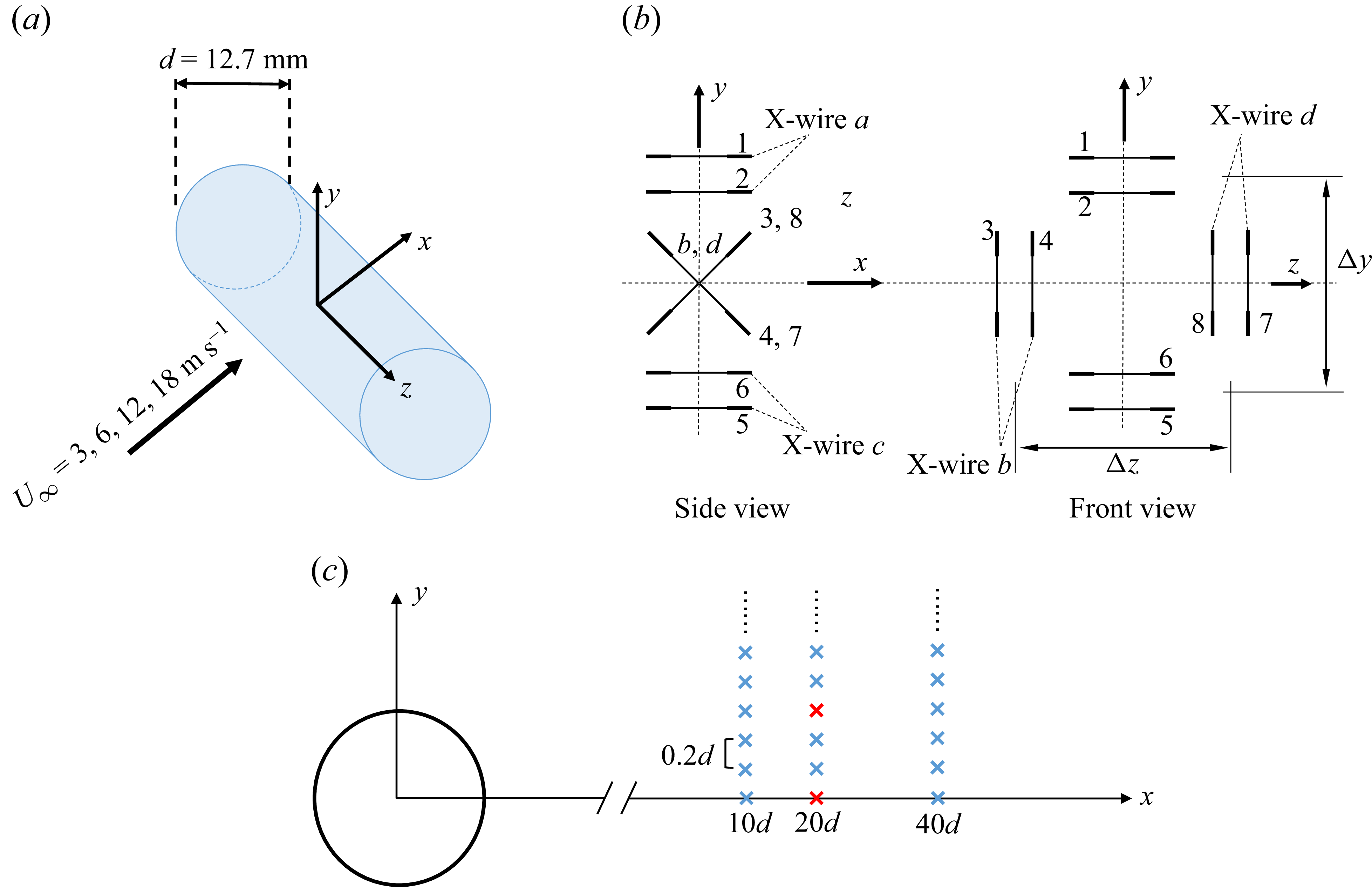
 (x/d,y/d)=(20,0)
 (20,0.6)
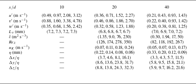
 u′
 v′
 w′
 Lv
 ε¯
 Reλ
 uK
 η
 Red=2500−15000
 ε¯

 Ruu
 Rvv
 Rww
 x/d=20
 y/d=0
 Red=2500
 −15000
 r
 Rvv
 Rww
 2%

 Red=15000
 x/d=20
 y/d=0−2.4
 d
 U∞
 ϕu(f)
 ϕv(f)
 ϕw(f)
 −5/3
 fcd/U∞≈0.2
 fc
 (fd/U∞)5/3
 ϕv(f)
 (fd/U∞)4.5/3
 y/d=1.9
 (fd/U∞)4.3/3
 y/d=2.4
 ϕv(f)
 ϕw(f)
 y/d⩾0.6
 log15
 log200
 log1500
 log20000

 Red=15000
 x/d=10−40
 y/d=0
 d
 U∞
 ϕu(f)
 ϕv(f)
 ϕw(f)
 −5/3
 x/d=20
 log20
 log200
 (fd/U∞)5/3
 ϕu(f)
 (fd/U∞)5.7/3
 x/d=10
 x/d=20
 log10
 log100
 ϕv(f)
 ϕw(f)

 Red=2500−15000
 x/d=20
 y/d=0
 d
 U∞
 ϕu(f)
 ϕv(f)
 ϕw(f)
 −5/3
 Red⩽10000
 log15
 log200
 log8000
 (fd/U∞)5/3
 Red⩽10000
 log10
 log100
 log1000
 Red=43300
 x/d=25
 y/d=0
 ϕv(f)
 ϕw(f)

 ϕv(f)
 d
 U∞
 x/d=20
 y/d=0
 Red=2500−15000
 Red⩽10000
 log7
 log50
 log300
 fd/U∞≳0.2
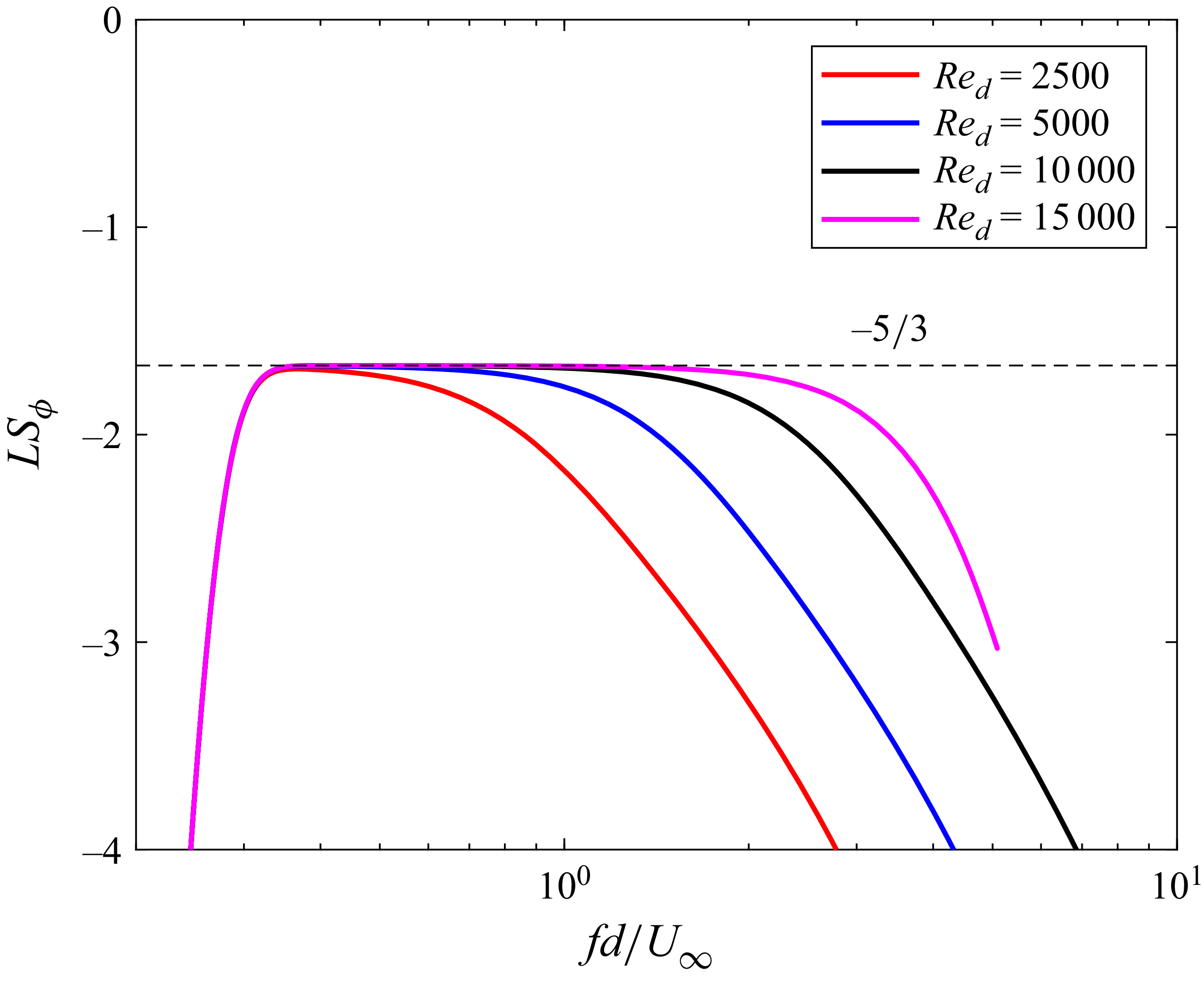
 (LSϕ=dlog(ϕv(f))/dlog(f))
 x/d=20
 y/d=0
 −5/3

 ϕu(f)
 Red=2500−15000
 x/d=10
 y/d=0
 d
 U∞
 −7/3
 −6.4/3
 −6.1/3
 −5.9/3
 −5.7/3
 Red⩽10000
 log7
 log50
 log300
 log2000
 (fd/U∞)m
 m[ϕu(f)∼f−m]
 Red⩽10000
 log4
 log20
 log100
 log400
 Red=7000
 x/d=10
 y/d=0

 ϕv(f)
 −7.3/3
 −6.5/3
 −6.2/3
 −5.6/3
 −5/3
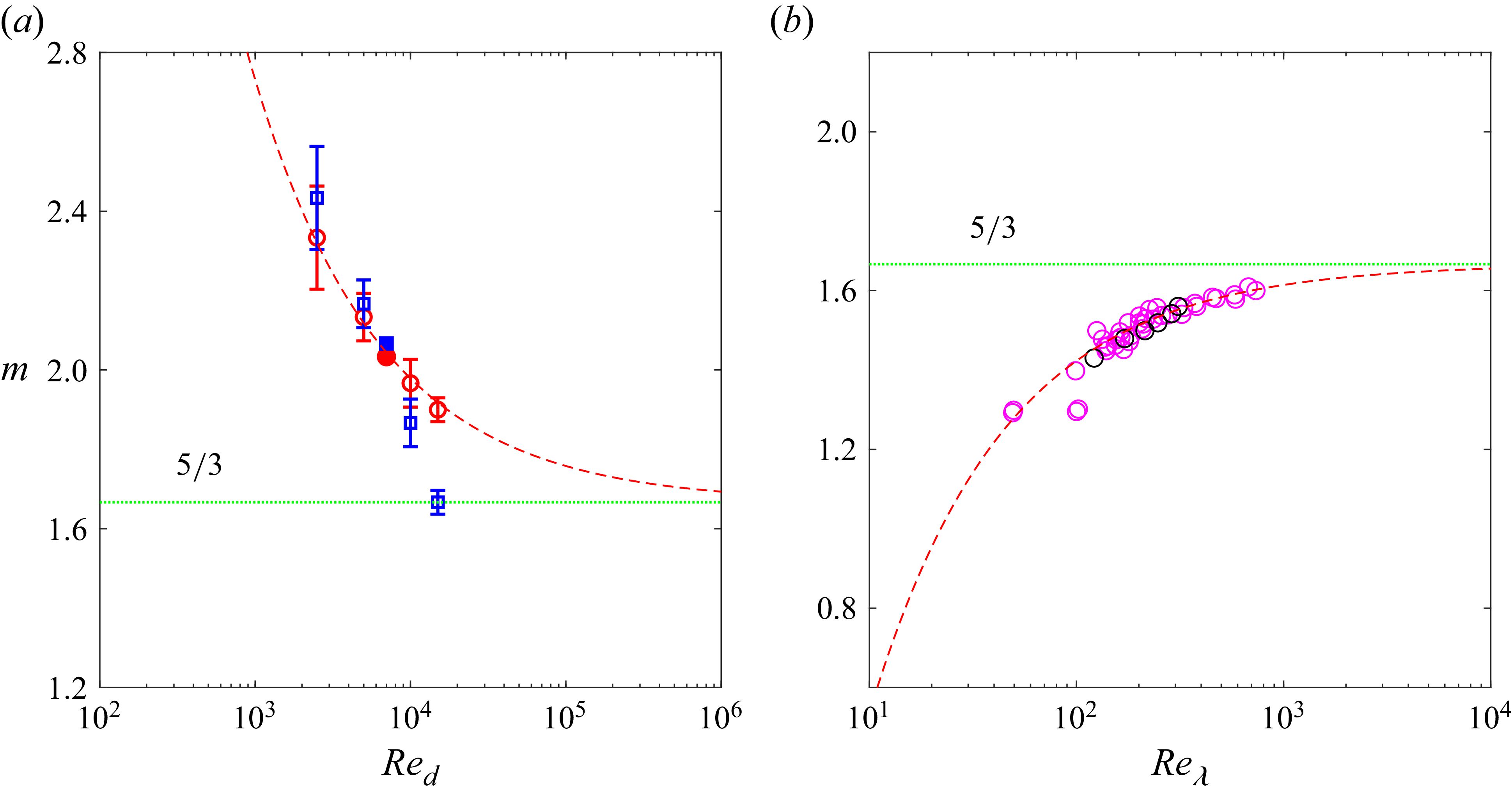
 m
 x/d=10
 y/d=0
 ∘
 ϕu(f)
 ◻
 ϕv(f)
 5/3+42.3Red−0.533
 ϕu(f)
 m
 5/3−5.25Reλ−2/3
 ϕu(κ1)

 ϕu(f)
 ϕv(f)
 x/d=6−10
 Red=2500−3900
 d
 U∞
 −5/3
 x/d=10
 Red=2500
 x/d=8
 Red=3900
 x/d=10
 Red=3900
 x/d=6
 Red=2500
 x/d=6
 Red=2500
 (fd/U∞)5/3

 ϕv(κ1)
 x/d=20
 y/d=0
 v′
 Lv
 uK
 η
 −5/3
 Reλ=57
 Reλ=433

 ϕu(κ1)
 ϕw(κ1)
 x/d=20
 y/d=0
 v′
 Lv
 uK
 η
 −5/3
 Reλ=57
 Reλ=433
 ϕu(κ1)
 log500

 ϕu(κ1)
 ϕv(κ1)
 ϕw(κ1)
 x/d=20
 y/d=0.6
 v′
 Lv
 uK
 η
 −5/3
 Reλ=57
 Reλ=433
 ϕw(κ1)
 ϕu(κ1)
 log300
 log50000
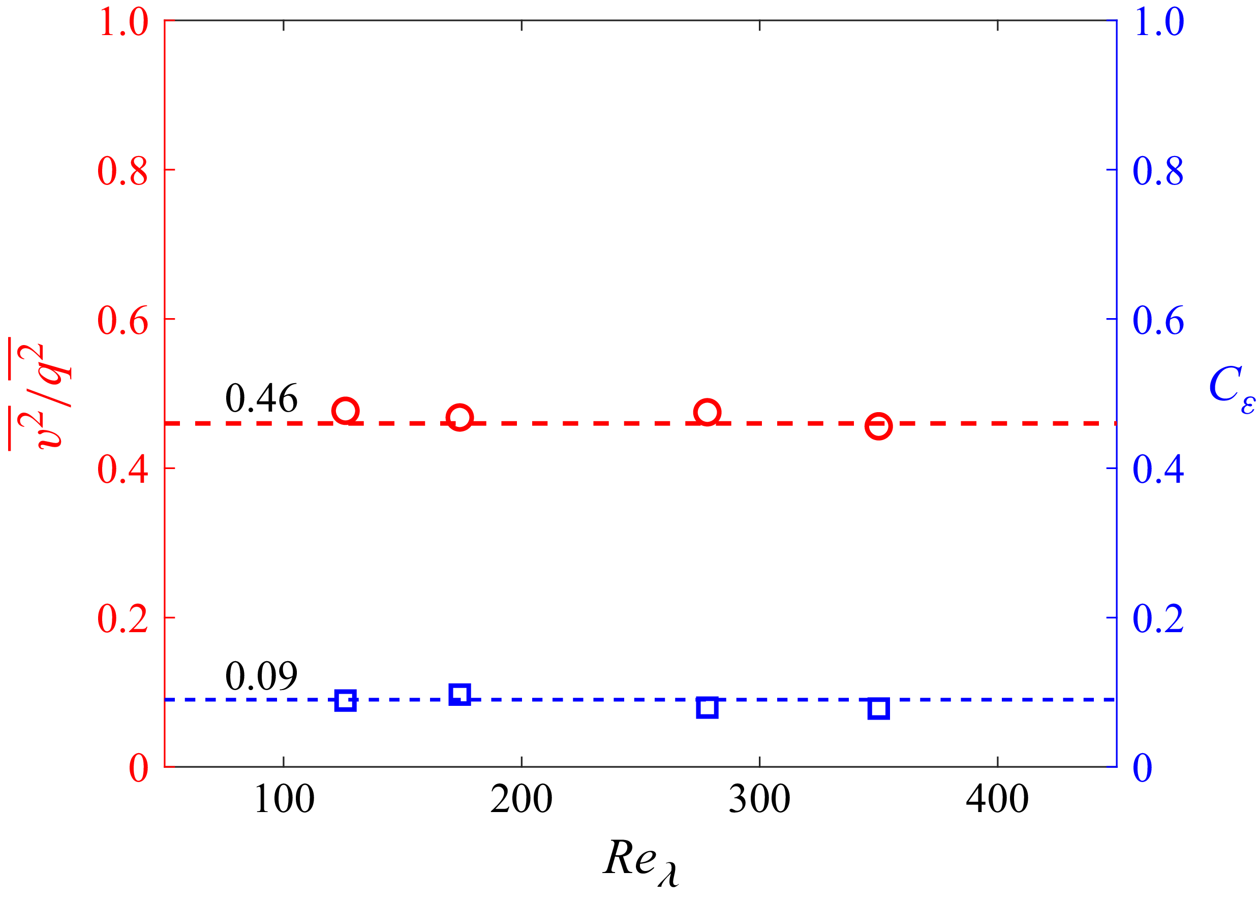
 v2¯/q2¯
 Cε
 Reλ
 x/d=20
 y/d=0

 v
 log
 x/d=20
 y/d=0.6
 Red=15000
 Lc
 ⟨(Δv)2⟩/v2¯
 (Δv~)2/v~2¯
 ⟨(Δv′)2⟩/v′2¯
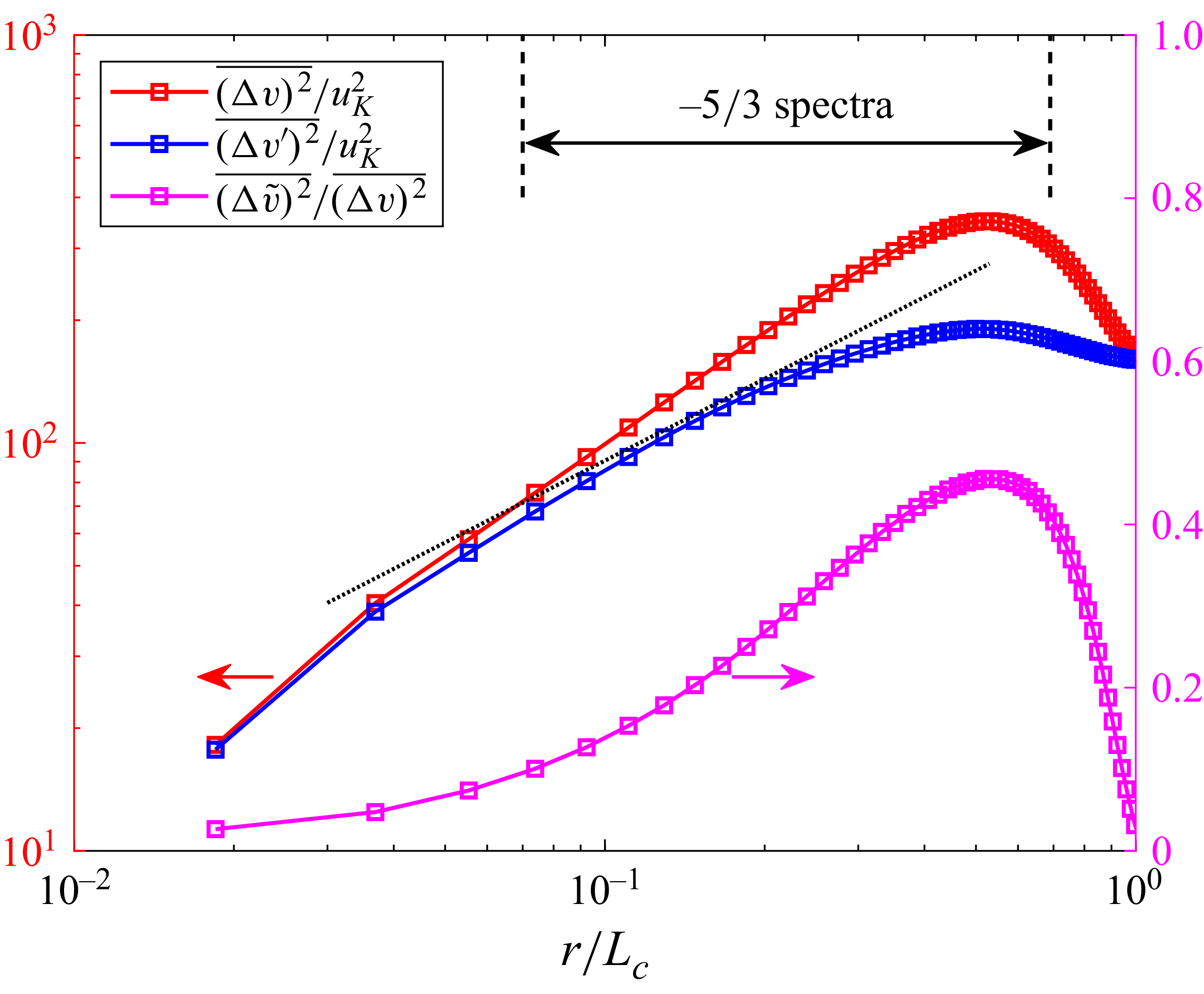
 ⟨(Δv)2⟩¯/uK2
 (Δv′)2¯/uK2
 (Δv~)2¯/⟨(Δv)2⟩¯
 x/d=20
 y/d=0.6
 Red=15000
 2/3
 −5/3
 0.07≲r/Lc≲0.69
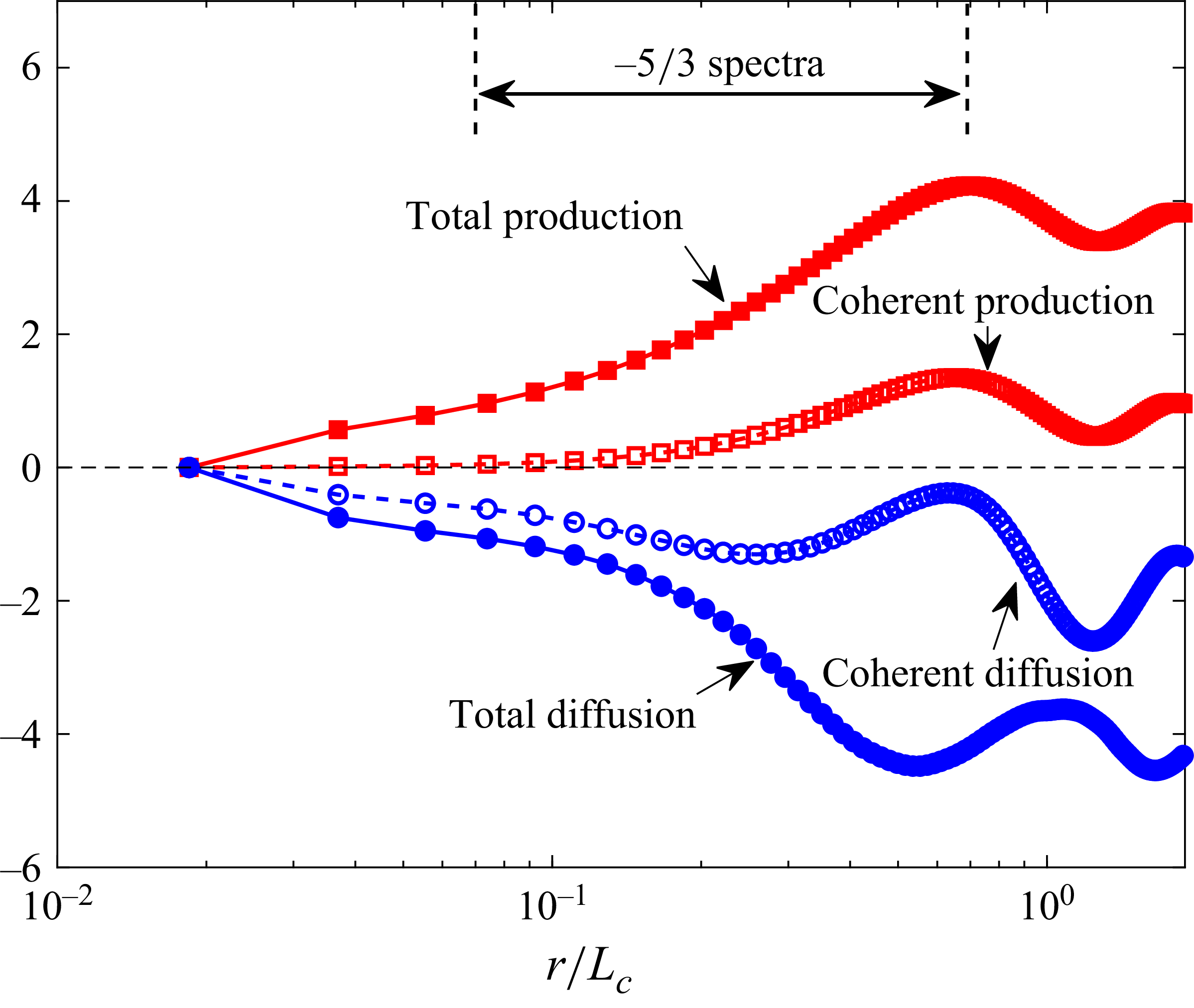
 (Δq)2¯
 x/d=20
 y/d=0.6
 (2/r2)∫0rs2ΔuΔv¯(∂U¯/∂y)ds
 (2/r2)∫0rs2(∂/∂y)(v(Δq)2¯)ds
 (Δq~)2¯
 (2/r2)∫0rs2Δu~Δv~¯(∂U¯/∂y)ds
 (1/r2)∫0rs2(∂/∂y)(∑v~(Δq~)2¯+2⟨∑v′Δq′⟩Δq~¯)ds
 ε¯r
 −5/3
 0.07≲r/Lc≲0.69
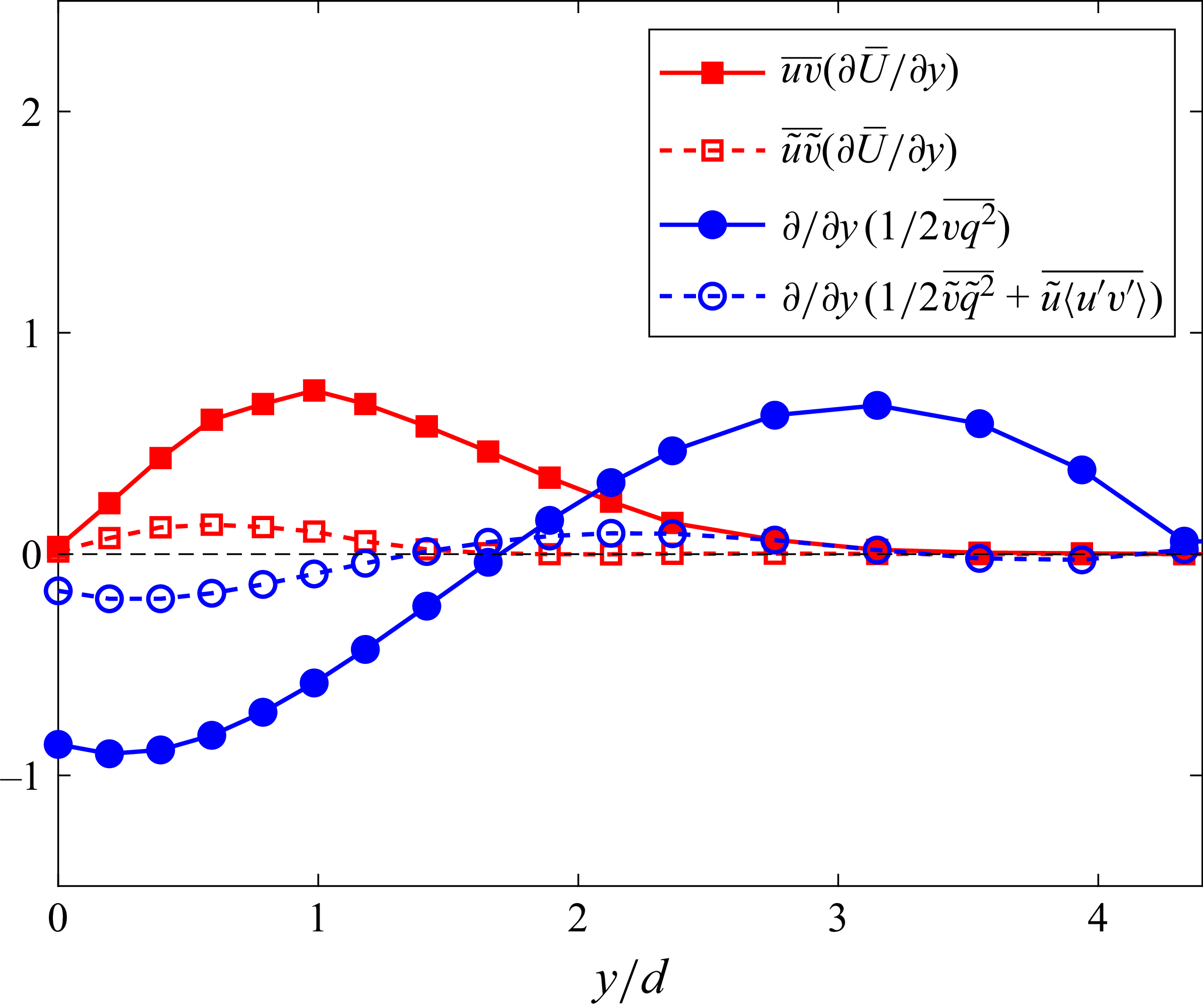
 uv¯(∂U¯/∂y)
 (1/2)((∂vq2¯)/∂y)
 q2¯
 x/d=20
 u~v~¯(∂U¯/∂y)
 (∂/∂y)((1/2)v~q~2¯+u~⟨u′v′⟩¯)
 q~2¯
 ε¯
 x/d=20
 y/d=0.6

 ε¯
 y/d=0
 x/d=20−40
 Red=2500−5000
 u
 Reλ=57
 Reτ
 u
 Reλ=433
 u
 y/d=0
 x/d=20−40
 Red=2500−5000
 x/d=40
 log500

 u
 x/d=20−40
 Red=2500−15000
 y/d=0
 u
 Reλ=57
 u
 Reλ=433


