1. Introduction
The study of elliptic problems involving nonlocal operators has been the subject of intense research in recent decades. From the perspective of applications, the inclusion of the nonlocal term allows for more realistic modelling of phenomena. For instance, a pioneering work in considering nonlocal models in Population Dynamics is attributed to [Reference Furter and Grinfeld16]. See also [Reference Alves, Delgado, Souto and Suárez6, Reference Hillen, Greese, Martin and de Vries20] and the references therein.
Conversely, from a mathematical standpoint, it is known that the inclusion of nonlocal terms leads to significant technical difficulties in the analysis. For instance, in many cases, the uniqueness of the solution is lost, even for the linear problem, as proven in [Reference Chipot10]. Additionally, classical papers such as [Reference Allegretto and Barabanova5] and [Reference Freitas and Sweers15] have established that some nonlocal operators do not satisfy the maximum principle.
However, few years ago, in [Reference Delgado, Suárez and Duarte13], the authors proved that the characterization of the maximum principle (see [Reference López-Gómez22]) is satisfied for the following nonlocal operator:
 \begin{equation*}
\mathfrak{L}u := -d\Delta u + c(x)u - \int_\Omega K(x,y)u(y)dy,
\end{equation*}
where  $\Omega \subset \mathbb{R}^N$,
 $N\ge 1$, is a bounded and regular domain, d > 0 is a constant, and K is a non-negative, non-trivial, continuous function.
This characterization is an important tool in the study of nonlinear Partial Differential Equations and was first established in the context of cooperative systems in [Reference López-Gómez and Molina-Meyer23]. We also mention [Reference López-Gómez22] and its references. Since then, it has been widely used, leading to extensions for other classes of operators. For instance, in [Reference Antón and López-Gómez7, Reference Peng and Zhao27], the authors establish a form for periodic parabolic operators; in [Reference Abreu, Morales-Rodrigo and Suárez1], a version for an elliptic operator with a nonlocal boundary condition is obtained. More recently, this characterization has been proved for elliptic interface problems in [Reference Maia, Morales-Rodrigo and Suárez25].
Inspired by these works, the first main goal of this paper is to extend this framework to the operator  $(\mathcal{L}-\int_\Omega K(x,y)\cdot dy, \mathfrak{B},\Omega)$, where
 $\Omega \subset \mathbb{R}^N$,
 $N\ge 1$, is a regular bounded domain of class C 2 such that
 $\partial \Omega = \Gamma_0 \cup \Gamma_1 $, with
 $\Gamma_0 \cap \Gamma_1 = \emptyset $ and
 $K \in L^\infty(\Omega\times \Omega)$. Moreover,
 \begin{equation*}\mathcal{L}u:= - \text{div}(A \nabla u) + \langle \vec b, \nabla u \rangle + c u\end{equation*}
is a uniformly elliptic operator, where  $A:=(a_{ij})_{1 \le i,j \le N}$ is a symmetric matrix with
 $a_{ij} \in W^{1,\infty}(\Omega)$,
 $\vec b:=(b_1,...,b_N) \in (L^{\infty}(\Omega))^N$, and
 $c \in L^{\infty}(\Omega)$. For simplicity, we will denote
 \begin{equation*}
\mathcal{L_I}u:= \mathcal{L}u - \int_\Omega K(x,y)u(y)dy.
\end{equation*}
The boundary operator  $\mathfrak{B}:C(\Gamma_0) \otimes C^1(\Gamma_1) \longrightarrow C(\partial \Omega)$ is given by
 \begin{equation*}\mathfrak{B}\psi :=
\left\{
\begin{array}{ll}
\mathfrak{D}\psi & \text{on } \Gamma_0,\\
\frac{\partial \psi}{\partial \eta} + \beta \psi& \text{on } \Gamma_1,
\end{array}
\right.
\end{equation*}
where  $\mathfrak{D}$ denotes de homogeneous Dirichlet boundary condition,
 $\eta:= A \cdot \vec{n}$ and
 $\vec{n}:=\vec{n}(x)$ stands for the outward unit normal to Ω at
 $x \in \partial\Omega$. (See Theorem 2.8).
As a consequence of this result, we can establish several properties of the associated principal eigenvalue
 \begin{equation}
\left\{
\begin{array}{ll}
\displaystyle \mathcal{L}u - \int_\Omega K(x,y)u(y)dy=\lambda u &\text{ in}\ \Omega,\\
\mathfrak{B}u=0 & \text{ on}\ \partial \Omega,
\end{array}\right.
\end{equation}
Subsequently, these results allow us to study the eigenvalue problem with a weight. The case K = 0 is well-known and was established for the first time in the celebrated paper [Reference Hess and Kato19]. More recently, in [Reference Wan-Tong, López-Gómez and Sun28], the authors proved an important convergence of the eigenvalues and the associated eigenfunctions for this class of operators when K = 0,  $\mathcal{L}=-\Delta$, and
 $\beta \ge 0$. In this work, we will remove all these restrictions (see Theorem 3.6).
The last main goal of this paper is to establish results on existence and uniqueness of positive strong solutions (in  $W^{2,p}(\Omega)$, p > N) for the following logistic equation with indefinite weight:
 \begin{equation}
\left\{
\begin{array}{ll}
\displaystyle \mathcal{L}u - \int_\Omega K(x,y)u(y)dy=\lambda m(x)u-b(x)f(u)u & \text{ in}\quad \Omega,\\
\mathfrak{B}u=0& \text{ on}\quad \partial \Omega,
\end{array}\right.
\end{equation}
where  $f:\mathbb{R} \to \mathbb{R}$ is a C 1 function,
 $b \in C(\overline{\Omega})$ is a non-negative function, and
 $m \in C(\overline{\Omega})$ that may change sign. We also analyse the pointwise behaviour of these solutions with respect to the parameter λ (see Section 5).
The equation (P) is a stationary reaction-diffusion model widely applied in Population Dynamics. In this context, Ω represents the habitat of a species whose density is given by u. The right-hand side of this equation corresponds to a logistic-type reaction term, the most common form used in the study of such phenomena, where b describes the carrying capacity and  $ \lambda m $ represents the local growth rate of the population. Allowing m to change sign enables the model to distinguish between favourable regions for the species (where m > 0) and unfavourable ones (where m < 0) (see [Reference Cantrell and Cosner9, Reference Wan-Tong, López-Gómez and Sun28]). The left-hand side of equation (P) represents the diffusion term. In this framework, the model incorporates both local diffusion (represented by the operator
 $ \mathcal{L} $) and nonlocal diffusion (expressed through the integral term). Specifically, the nonlocal term accounts for the dispersal of individuals ‘jumping’ from position
 $ y \in \Omega $ to
 $ x \in \Omega $ (see [Reference Cintra, Morales-Rodrigo and Suárez11, Reference Delgado, Suárez and Duarte13, Reference Hillen, Greese, Martin and de Vries20]). Finally, the boundary condition reflects the habitat’s interaction with its surroundings: part of the boundary (Γ0) is inhospitable for the species, while, in another portion (Γ1), act as barriers (β = 0), an inflow region (β < 0), or outflow region (β > 0). These considerations make the model more realistic from an application perspective, while also introducing technical challenges in its analysis.
The study of (P) with  $K \equiv 0$ goes back to [Reference Ouyang26], where the existence and uniqueness of positive solutions were established for the Laplacian operator under homogeneous Dirichlet boundary conditions and
 $ m \equiv 1 $. In [Reference Aleja, Antón and López-Gómez4], the authors conducted this study in a more general setting using bifurcation and sub- and supersolution methods. Subsequently, the asymptotic behaviour of the solutions with respect to λ was investigated in [Reference Du and Huang14, Reference García-Melián, Gómez-Reñasco, López-Gómez and Sabina de Lis17, Reference López-Gómez and Sabina de Lis24] for the case
 $m \equiv 1$. Only recently, in [Reference Wan-Tong, López-Gómez and Sun28], this analysis was extended to the case where m changes sign and with mixed boundary conditions. It should be noted that in [Reference Wan-Tong, López-Gómez and Sun28], the authors consider the Laplacian operator and
 $\beta \geq 0$. Both hypotheses are removed here. To the best of our knowledge, the problem (P) with a nonlocal term has only been studied in [Reference Cintra, Morales-Rodrigo and Suárez11].
We emphasize that the results presented in this paper substantially generalize several previous studies in the literature. For instance, regarding the problem (P), we highlight that the presence of the integral term and the sign-changing functions m and β introduce technical challenges to the analysis, in addition to being ecologically interesting as they model more realistic scenarios. Furthermore, the nonlocal diffusion term leads to an asymptotic behaviour that is entirely different from the local case (see  $\S$ 5 and Remark 5.4).
Hypotheses: Throughout this work, we will assume the following:
(f1)
 $f: \mathbb{R} \longrightarrow \mathbb{R} $ is a C 1 function such that
$ f(0) = 0,$
$f'(s) \gt 0 $ for all s > 0 and
\begin{equation*}
\lim_{s \to \infty} f(s) = +\infty.
\end{equation*}


 $b \in C(\overline{\Omega})$ is a non-negative function that may vanish on some subset of
 $\Omega.$ Thus, we distinguish between two cases:
(b0)
$\min_{x \in \overline{\Omega}} b(x) \gt 0$ or(b1) The set
\begin{equation*}\Omega_0:=\mathrm{int}\{x \in \Omega;\, b(x)=0\}\end{equation*}


is a nonempty regular subdomain of Ω such that
 \begin{equation*}\mathrm{dist}(\partial \Omega, \partial \Omega_0 \cap \Omega) \gt 0. \end{equation*}
In  $\S$ 3 and 5, in addition to hypothesis (b 1), we shall also assume that
(m1) There exists
$ x_0 \in \Omega_0 $ such that
$ m(x_0) \gt 0$.


Finally, we mention that an additional hypothesis regarding a principal eigenvalue is also assumed in the last three sections.
Notations:
•
$W^{k,p}_{\Gamma_0}(\Omega)=\{u\in W^{k,p}(\Omega);\, u=0 \text{ on } \Gamma_0\};$•
$ C^{1}_{\mathfrak{B}}(\overline{\Omega}) = \{u \in C^{1}(\overline{\Omega}); \mathfrak{B}u = 0 \text{ on } \partial \Omega \}; $•
$\mathcal P = \{u \in C^{1}_{\mathfrak{B}}(\overline{\Omega}); u \ge 0 \text{ in } \Omega \}; $•
$ \text{int}(\mathcal P) = \left\{u \in \mathcal{P}; u(x) \gt 0, \forall x \in \Omega \cup \Gamma_1 \quad \text{and} \quad \frac{\partial u}{\partial \eta}(x) \lt 0, \forall x \in \Gamma_0 \right\}; $• Given
$ u \in C(\Omega) $, u > 0 means that
$ u(x) \geq 0 $ in Ω and u ≠ 0;• Given
$ u \in C^1_\mathfrak{B}(\overline{\Omega}) $,
$u\gg0$ means that
$u(x) \gt 0,$ for all
$x\in \Omega\cup\Gamma_1,$ and
$\frac{\partial u}{\partial \eta}(x) \lt 0,$ for all
$x\in u^{-1}(0)\cap \Gamma_{0}$;•
$\mathcal{L_I}u:= \mathcal{L}u -\displaystyle \int_\Omega K(x,y)u(y)dy$ and
$\mathcal{L_I}_0u:= \mathcal{L}u -\displaystyle \int_{\Omega_0} K(x,y)u(y)dy.$•
$\langle\cdot ,\cdot \rangle_{L^2(\Omega)}$: denote the standard inner product in
$L^2(\Omega)$.


The outline of this paper is as follows. In  $\S$ 2, we prove the characterization of the maximum principle for
 $(\mathcal{L_I}, \mathfrak{B}, \Omega)$ and obtain important properties of the associated principal eigenvalue. Section 3 is dedicated to the study of the eigenvalue problem with weight. The results on the existence and uniqueness of positive solutions of (P) are established in
 $\S$ 4, while the asymptotic behaviour of the solutions is analysed in
 $\S$ 5.
2. Characterization of the maximum principle and applications
Our goal in this section is to provide a characterization of the Maximum Principle for the operator  $\mathcal{L_I}$ with mixed boundary conditions. We highlight that the results presented herein extend those obtained in [Reference López-Gómez22] and [Reference Delgado, Suárez and Duarte13].
To facilitate readability, the subsections are organized as follows: in  $\S$ 2.1, we analyse the existence and uniqueness of solutions for a linear problem associated with
 $(\mathcal{L_I}, \mathfrak{B}, \Omega)$. Section 2.2 focuses on the existence and uniqueness of the principal eigenvalue of
 $(\mathcal{L_I}, \mathfrak{B}, \Omega)$ (see (EP)). In
 $\S$ 2.3, we establish the characterization of the Maximum Principle for
 $(\mathcal{L_I}, \mathfrak{B}, \Omega)$. Finally,
 $\S$ 2.4 is devoted to studying key properties of this principal eigenvalue. The concept presented below will be widely used throughout this work.
Definition 2.1. Let  $ u \in W^{2,p}(\Omega)$, p > N. Then, u is said to be a supersolution of
 $(\mathcal{L_I}, \mathfrak{B}, \Omega)$ if
 \begin{equation*}
\left\{
\begin{array}{ll}
\mathcal{L_I} u \ge 0 &\text{ in } \Omega, \\
\mathfrak{B} u \ge 0 &\text{ on } \partial \Omega.
\end{array}\right.
\end{equation*}
If any of these inequalities is strict, u is said to be a strict supersolution of  $(\mathcal{L_I}, \mathfrak{B}, \Omega)$.
2.1. Linear problem
To study problem (EP), we must analyse the existence of weak solutions for the following problem:
 \begin{equation}
\left\{
\begin{array}{ll}
(\mathcal{L_I} + M)u = g(x) & \text{ in } \Omega, \\
\mathfrak{B}u = 0 & \text{ on } \partial \Omega,
\end{array}\right.
\end{equation}
where M > 0 and  $ g \in L^2(\Omega) $. For this purpose, let us consider the bilinear form
 $\mathfrak{b}_M : W^{1,2}_{\Gamma_0}(\Omega) \times W^{1,2}_{\Gamma_0}(\Omega) \rightarrow \mathbb{R} $ defined as
 \begin{align*}
\mathfrak{b}_M(u, v) &:= \int_{\Omega} \langle A \nabla u, \nabla v \rangle + \int_{\Omega} \left( \langle \vec b, \nabla u \rangle + uc + uM \right)v \\
&
\qquad+ \int_{\Gamma_1} \beta uv \, dS - \int_{\Omega} \int_{\Omega} v K(x, y) u(y) \, dy.
\end{align*}
We say that  $ u_0 \in W_{\Gamma_0}^{1,2}(\Omega) $ is a weak solution of problem (2.1) if
 \begin{equation*} \mathfrak{b}_M(u_0, v) = \int_{\Omega} gv, \quad \forall\,\, v \in C_{\Gamma_0}^{\infty}(\Omega). \end{equation*}
The bilinear form  $\mathfrak{b}_M$ is continuous, and the following properties hold:
Lemma 2.2. Suppose  $\beta \ge 0$. Then, there exists
 $ M_0 \gt 0 $ such that
 \begin{equation*} \mathfrak{b}_M(u, u) \ge \frac{\theta}{2}\|u\|^2_{W_{\Gamma_0}^{1,2}(\Omega)} \quad \forall u \in W_{\Gamma_0}^{1,2}(\Omega), \quad M \ge M_0,\end{equation*}
where θ > 0 denotes the ellipticity constant of  $\mathcal{L}$ in Ω.
Proof. Let  $u \in W^{1,2}_{\Gamma_{0}}(\Omega)$. Since
 $\beta \ge 0$, we have
 \begin{equation}
\mathfrak{b}_M(u,u)
\ge \int_{\Omega}\langle \nabla u,A\nabla u\rangle+\int_{\Omega}u \bigg(\langle \vec b,\nabla u\rangle+uc+uM\bigg)-\int_{\Omega}\int_{\Omega}uK(x,y)u(y)dy.
\end{equation}
We will obtain estimates for each of the above terms. Since  $\mathcal{L}$ is uniformly elliptic in Ω, we get
 \begin{equation}
\int_{\Omega} \langle \nabla u, A \nabla u \rangle \ge \theta \int_{\Omega} \langle \nabla u, \nabla u \rangle = \theta \| \nabla u \|^{2}_{L^{2}(\Omega)}.
\end{equation}
Moreover, by using Young’s inequality, we find that
 \begin{equation}
\int_{\Omega} \langle \vec b, \nabla u \rangle u \ge -\frac{\|\vec b\|_{L^{\infty}(\Omega)}}{2} \left( \epsilon \| u \|_{L^{2}(\Omega)}^2 + \frac{\|\nabla u \|_{L^{2}(\Omega)}^2}{\epsilon} \right),
\end{equation}
where ϵ is a positive constant. Furthermore,
 \begin{equation}
\int_{\Omega} (uc + uM)u \ge (M + \inf_{\Omega} c) \int_{\Omega} u^2 = (M + \inf_{\Omega} c) \| u \|^{2}_{L^{2}(\Omega)}.
\end{equation}
Finally, there exists a positive constant  $C_1 \gt 0$ such that
 \begin{equation}
-\int_{\Omega} \int_{\Omega} u K(x, y) u(y) \, dy \ge -\| K \|_{L^{\infty}(\Omega\times\Omega)} C_{1} \| u \|^2_{L^{2}(\Omega)}.
\end{equation}
Consequently, substituting (2.3), (2.4), (2.5), and (2.6) into (2.2), we have that
 \begin{align*}\begin{array}{ll}
\mathfrak{b}_M(u, u) &\ge
\left( \theta - \frac{\|\vec b\|_{L^{\infty}(\Omega)}}{2 \epsilon} \right) \|\nabla u \|^{2}_{L^{2}(\Omega)} \\
&+ \left( M + \inf_{\Omega} c - \frac{\|\vec b\|_{L^{\infty}(\Omega)}}{2} \epsilon - \| K \|_{L^{\infty}(\Omega\times\Omega)} C_{1} \right) \| u \|^{2}_{L^{2}(\Omega)}.
\end{array}\end{align*}
Choose ϵ > 0 such that  $\theta - \|\vec b\|_{L^{\infty}(\Omega)}/2 \epsilon = \theta/2 \gt 0,$ and define
 $M_{0} := -\inf_{\Omega} c + \| \vec b \|_{L^\infty(\Omega)}\epsilon/2 + \| K \|_{L^{\infty}(\Omega\times\Omega)} C_{1} + \theta/2.$ Then, for all
 $M \ge M_{0}$, we have that
 \begin{equation*}
\mathfrak{b}_M(u, u) \ge \frac{\theta}{2} \left( \|\nabla u \|^{2}_{L^{2}(\Omega)} + \| u \|^{2}_{L^{2}(\Omega)} \right) = \frac{\theta}{2} \| u \|^2_{W^{1,2}_{\Gamma_{0}}(\Omega)}.
\end{equation*}
This concludes the proof.
From now on, we will consider  $M_0\ge0$ as in Lemma 2.2. As a consequence of this proposition, we can apply the Lax–Milgram Theorem to ensure the following existence result for the solution of (2.1).
Proposition 2.1.
Suppose  $\beta \ge 0$, and let
 $M\ge M_0$. Then for each
 $g \in L^2(\Omega)$, the problem (2.1) has a unique weak solution,
 $u \in W^{1,2}_{\Gamma_0}(\Omega).$
We now consider the case where β changes sign. To address this, we will employ the following auxiliary result, which arises as a consequence of the regularity of Ω.
Lemma 2.3. There exists a constant  $\widetilde{M} \gt 0$ such that, for every
 $M \geq \widetilde{M}$, the operator
 $(\mathcal{L_I} + M, \mathfrak{B}, \Omega)$ admits a strict supersolution
 $h \in C^{2}(\overline{\Omega})$, satisfying
 $h(x) \gt 0$ for all
 $x \in \overline{\Omega}$.
Proof. First, note that since Ω is of class C 2, by [Reference López-Gómez22, Lemma 2.1], there exist  $\psi \in C^{2}(\bar{\Omega})$ and γ > 0 such that
 \begin{equation*}\frac{\partial\psi}{\partial\eta}(x)\ge\gamma, \quad\forall x\in\Gamma_{1}.\end{equation*}
Defining  $h(x)= e^{\omega \psi(x)}$, where ω > 0 is a constant, we observe that
 $h(x) \gt 0$ for all
 $ x \in \Omega $. Moreover, on Γ1 we find
 \begin{equation*}
\mathfrak{B}h=\frac{\partial h}{\partial \eta}+\beta h=\omega h\frac{\partial\psi}{\partial\eta}+\beta h=h(\omega\frac{\partial\psi}{\partial\eta}+\beta)\ge h(\omega\gamma+\beta) \gt 0,
\end{equation*}
for all  $\omega \gt -\inf_{\Gamma_1} \beta/\gamma=:\omega_0$.
On the other hand, due to the regularity of the coefficients of  $\mathcal{L_I}$, we have
 $\mathcal{L_I}h \in L^\infty(\Omega)$. Consequently,
 \begin{equation*}(\mathcal{L_I}+M)h \ge -\|\mathcal{L_I}h\|_{L^{\infty}(\Omega)} + M \inf h \gt 0 \quad \mbox{in }\Omega,\end{equation*}
whenever  $M \gt \Arrowvert{\mathcal L}_{\mathcal I}h{\Arrowvert_{L^\infty(\Omega)}/\inf h}=:\widetilde M$. Hence, h satisfies the required condition.
From this point onwards, we assume  $M \gt \widetilde{M}$ and define the following auxiliary elliptic operator:
 \begin{equation*}
\mathcal{L_{I}}_{h}:=-\text{div}(A\nabla \cdot)+\langle \vec b_h,\nabla\cdot\rangle+c_h\cdot-\int_{\Omega}K_h(x,y)\cdot dy,
\end{equation*}
where h is the function given by the previous lemma,
 \begin{equation*}
\vec b_h:=\vec b-\frac{2}{h}A\nabla h,\quad
c_h:=\frac{\mathcal{L}h}{h}\quad\text{and }\quad K_h(x,y):=K(x,y)\frac{h(y)}{h(x)}.
\end{equation*}
Note that  $\vec b_h\in(L^{\infty}(\Omega))^{N}$ and
 $c_h\in L^{\infty}(\Omega).$ We further define
 \begin{equation*}
\mathfrak{B}_h:=\left\{
\begin{array}{ll}
\mathfrak{D} &\text{on }\Gamma_{0}, \\
\frac{\partial\cdot}{\partial\eta}+\beta_h &\text{on }\Gamma_{1},
\end{array}
\right.
\end{equation*}
where  $\beta_h:=\mathfrak{B}h/h$. We emphasize that, since h is a positive strict supersolution of
 $(\mathcal{L_I}+M,\mathfrak{B},\Omega)$,
 $M \gt \widetilde{M}$, then
 $\beta_h \gt 0$.
With these considerations, by direct calculation, given  $u \in W_{\Gamma_0}^{2,p}(\Omega),$
 $p \gt N,$ and defining
 $v:=u/h$, we obtain
 \begin{equation}
\mathcal{L_I}u=\mathcal{L_I}(hv)=h\mathcal{L_I}_hv\,\text{ in } \Omega \quad \mbox{and} \quad \mathfrak{B}u=h\mathfrak{B}_h\frac{u}{h}\,\text{ on }\partial\Omega .
\end{equation}
Finally, we define the following auxiliary problem:
 \begin{equation}
\left\{\begin{array}{ll}
(\mathcal{L_I}_h+M)v=\displaystyle \frac{g}{h}&\text{ in }\Omega,\\
\mathfrak{B}_hv=0&\text{ on }\partial\Omega.
\end{array} \right.
\end{equation}
Let us now relate the weak solutions of problems (2.1) and (2.8). To do this, we first prove the following result:
Lemma 2.4. Consider
 \begin{equation*}\mathfrak{b}_M,\mathfrak{b}_h:W^{1,2}_{\Gamma_{0}}(\Omega)\times W^{1,2}_{\Gamma_{0}}(\Omega)\longrightarrow \mathbb{R}\end{equation*}
as the bilinear forms associated with (2.1) and (2.8), respectively. Then, for all  $v,w\in W^{1,2}_{\Gamma_{0}}(\Omega)$,
 \begin{equation*}\mathfrak{b}_M(hv,\frac{w}{h})=\mathfrak{b}_h(v,w).\end{equation*}
Proof. Consider  $\mathfrak{b}_0, \mathfrak{b}_{0h}:W^{1,2}_{\Gamma_{0}}(\Omega)\times W^{1,2}_{\Gamma_{0}}(\Omega)\longrightarrow \mathbb{R}$, the bilinear forms given by
 \begin{equation*}\mathfrak{b}_0(v,w):=\int_{\Omega}\langle \nabla w,A\nabla v\rangle+\int_{\Omega}w \bigg(\langle \vec b,\nabla v\rangle+vc+vM\bigg)+\int_{\Gamma_{1}}w\beta vdS\end{equation*}
and
 \begin{equation*}\mathfrak{b}_{0h}(v,w):=\int_{\Omega}\langle\nabla w,A\nabla v\rangle+\int_{\Omega}w \bigg(\langle \vec b_h,\nabla v\rangle+vc_h+vM\bigg)
+\int_{\Gamma_{1}}w\beta_h vdS.\end{equation*}
By [Reference López-Gómez22, Lemma 4.2], it holds for all  $v,w\in W^{1,2}_{\Gamma_{0}}(\Omega)$,
 \begin{equation*}\mathfrak{b}_0(hv,\frac{w}{h})=\mathfrak{b}_{0h}(v,w).\end{equation*}
Thus
 \begin{equation*}
\mathfrak{b}_M(hv,\frac{w}{h})= \mathfrak{b}_{0h}(v,w)-\int_{\Omega}\int_{\Omega}wK_h(x,y)v(y)dy =\mathfrak{b}_h(v,w).
\end{equation*}
The next result establishes a relation between the weak solutions of (2.1) and (2.8).
Proposition 2.2.
Let  $h\in C^2(\overline{\Omega})$ be as in Lemma 2.3. Then, a function
 $v \in W^{1,2}_{\Gamma_{0}}(\Omega)$ is a weak solution of (2.8) if and only if
 $u:=hv \in W^{1,2}_{\Gamma_{0}}(\Omega)$ is a weak solution of (2.1).
Proof. Suppose that  $v\in W^{1,2}_{\Gamma_0}(\Omega)$ is a weak solution of (2.8). Defining u = hv, by Lemma 2.4, it holds that
 \begin{equation*}\mathfrak{b}_M(u,\frac{\phi}{h})=\mathfrak{b}_M(hv,\frac{\phi}{h})=\mathfrak{b}_h(v,\phi)=\langle \frac{g}{h},\phi\rangle_{L^{2}(\Omega)}, \quad\forall \phi\in C^{\infty}_{\Gamma_{0}}(\Omega).\end{equation*}
Since  $C^{\infty}_{\Gamma_0}(\Omega)$ is dense in
 $W^{1,2}_{\Gamma_0}(\Omega)$, it follows that
 \begin{equation*}
\mathfrak{b}_M(u,\psi)=\langle g,\psi\rangle_{L^{2}(\Omega)}, \quad \forall \psi\in C^{\infty}_{\Gamma_{0}}(\Omega),
\end{equation*}
which shows that  $u\in W^{1,2}_{\Gamma_0}(\Omega)$ is a weak solution of (2.1).
Conversely, suppose  $u\in W^{1,2}_{\Gamma_0}(\Omega)$ is a weak solution of (2.1) and define
 $v:=u/h$. For all
 $\phi\in C^{\infty}_{\Gamma_{0}}(\Omega),$ we have
 $\phi/h\in C^{2}_{\Gamma_0}(\Omega)\subset W^{1,2}_{\Gamma_0}(\Omega).$ Using again the density of
 $C^{\infty}_{\Gamma_0}(\Omega)$ in
 $W^{1,2}_{\Gamma_0}(\Omega)$, there exists a sequence
 $\psi_n \in C^{\infty}_{\Gamma_0}(\Omega)$ such that
 \begin{equation*}\psi_n\to \frac{\phi}{h}\text{ in }W^{1,2}_{\Gamma_0}(\Omega).\end{equation*}
Thus, by definition of weak solution, u verifies
 \begin{equation*}
\mathfrak{b}_M(u,\psi_n) = \mathfrak{b}_M(hv,\psi_n) = \langle u, \psi_n\rangle_{L^2(\Omega)}.
\end{equation*}
Letting  $n\to \infty$ in above equality, it becomes apparent that
 \begin{equation*}
\mathfrak{b}_M(hv,\frac{\phi}{h})=\langle g,\frac{\phi}{h}\rangle_{L^{2}(\Omega)}=\langle \frac{g}{h},\phi\rangle_{L^{2}(\Omega)},\quad \forall \phi\in C^{\infty}_{\Gamma_{0}}(\Omega).
\end{equation*}
By Lemma 2.4, this is equivalent to
 \begin{equation*}\mathfrak{b}_h(v,\phi)=\langle \frac{g}{h},\phi\rangle_{L^{2}(\Omega)}, \quad \forall \phi\in C^{\infty}_{\Gamma_{0}}(\Omega).\end{equation*}
Therefore, v is a weak solution of (2.8).
As a consequence, we have the following result:
Theorem 2.5. Let  $M\ge \max\{M_0, \widetilde{M}\}$. Then for each
 $g \in L^2(\Omega)$, the problem (2.1) has a unique weak solution.
Proof. Let  $g \in L^2(\Omega)$. Since
 $\beta_h\ge0$, it follows from Proposition 2.1 that there exists a unique weak solution,
 $v\in W^{1,2}_{\Gamma_0}(\Omega)$, to the problem (2.8). Now, by Proposition 2.2, we have that
 $u:=vh$ is the unique weak solution to the problem (2.1), where h is as in Lemma 2.3.
2.2. Principal eigenvalue
In this section, we will establish the existence of the principal eigenvalue of (2.1) via the Krein Rutman Theorem. We begin by presenting a maximum principle result, which provides a characterization of supersolutions of  $(\mathcal{L_I},\mathfrak B,\Omega)$
Proposition 2.3.
Suppose that  $(\mathcal{L_I},\mathfrak{B},\Omega)$ has a positive supersolution
 $h\in W^{2,p}(\Omega),$ p > N. Then, any supersolution
 $u\in W^{2,p}(\Omega),$
 $p \gt N,$ of
 $(\mathcal{L_I},\mathfrak{B},\Omega)$ must satisfy one of the following alternatives:
A1. u = 0 in Ω.
A2.
$u\gg0$.A3. There exists a constant ρ < 0 such that
\begin{equation*}
u=\rho h\text{ in }\overline{\Omega}.
\end{equation*}In this case,
$\Gamma_{0}=\emptyset$ and
\begin{equation*}
u(x) \lt 0,\quad \forall x\in\overline{\Omega}.
\end{equation*}Moreover, τ = 0 must be the only eigenvalue for a positive function of the problem
\begin{equation*}
\left\{
\begin{array}{ll}
\mathcal{L_I}\varphi=\tau\varphi& \text{ in }\Omega,\\
\mathfrak{B}\varphi=0& \text{ on }\partial \Omega.
\end{array}\right.
\end{equation*}


Proof. First, observe that  $h\ge0$ is also a supersolution of
 $(\mathcal{L},\mathfrak B,\Omega),$ since
 $\mathcal{L}h\ge \mathcal{L_I}h\ge0$ in Ω.
Now, let  $u\in W^{2,p}(\Omega)$, p > N, be a supersolution of
 $(\mathcal{L_I},\mathfrak B,\Omega)$. If
 $u\ge0$, then u is also a supersolution of
 $(\mathcal{L},\mathfrak B,\Omega)$, and we can apply Theorem 2.4 from [Reference López-Gómez22] to conclude the result.
Suppose instead that there exists some  $x_-\in\Omega$ such that
 $u(x_-) \lt 0.$ Define
 \begin{equation*}\Lambda:=\{\lambda \gt 0; v_{\lambda}(x):=u(x)+\lambda h(x)\ge0,\,\, x\in\Omega\}\end{equation*}
and  $\mu:=\inf\Lambda \gt 0. $ Then
 $v_\mu\ge0$ satisfies
 \begin{equation*}
\left\{
\begin{array}{ll} \mathcal{L}v_\mu\geq\mathcal{L_I}v_\mu=\mathcal{L_I}u+\mu\mathcal{L_I}h\ge0&\text{ in } \Omega,\\
\mathfrak{B}v_\mu=\mathfrak B u+\mu\mathfrak B h\ge0&\text{ on }\partial \Omega.
\end{array}\right.
\end{equation*}
Thus, vµ is a supersolution of  $(\mathcal{L},\mathfrak B,\Omega)$. By following the same steps as in the proof of [Reference López-Gómez22, Theorem 2.4], we conclude that
 $v_\mu = 0$, which ensures that alternative A3 holds.
Let  $M \ge \max\{M_0,\widetilde{M}\}$. By Theorem 2.5, we can define
 $T_M:C^{1}_{\mathfrak{B}}(\overline{\Omega})\longrightarrow C^{1}_{\mathfrak{B}}(\overline{\Omega})$, the solution operator associated with problem (2.1).
Proposition 2.4.
For each  $M \ge \max \{M_0, \widetilde{M}\}$, TM is well-defined, linear, compact, and strongly positive.
Proof. We begin by showing that TM is well-defined and compact. Let  $g\in C^{1}_{\mathfrak{B}}(\overline{\Omega})$. By Theorem 2.5, there exists a unique
 $u\in W_{\Gamma_0}^{1,2}(\Omega)$ which is the weak solution of problem (2.1). Moreover, since
 $g\in C^{1}_{\mathfrak{B}}(\overline{\Omega})$, it follows that
 $g\in L^\infty(\Omega)$. Define
 $U(x)=\int_{\Omega}K(x,y)u(y)dy$. Then,
 $U\in L^{\infty}(\Omega)$ and, consequently, u is also a weak solution of
 \begin{equation*}
\left\{\begin{array}{ll}
(\mathcal{L}+M)u=g(x)+U(x)&\text{ in }\Omega,\\
\mathfrak{B}u=0&\text{ on }\partial\Omega.
\end{array}
\right.
\end{equation*}
By elliptic regularity,  $u\in W^{2,p}(\Omega)$ for all
 $p\ge1$. The compact Sobolev embedding theorem then implies that
 $u\in C^{1}_{\mathfrak{B}}(\overline{\Omega})$. This establishes that TM is well-defined and compact. The linearity of TM follows from the linearity of
 $\mathcal{L_I}+M$.
It remains to prove that TM is strongly positive. To this end, consider  $g\in \mathcal P\setminus \{0\}.$ Then
 $u=T_Mg$ satisfies
 \begin{equation*}
\left\{\begin{array}{ll}
(\mathcal{L_I}+M)u=g \gt 0 &\text{ in }\Omega,\\
\mathfrak{B}u=0 &\text{ on }\partial\Omega.
\end{array}
\right.
\end{equation*}
Thus, u ≠ 0 is a supersolution of  $(\mathcal{L_I} + M, \mathfrak{B}, \Omega)$. By Lemma 2.3, there exists a supersolution
 $h \in C^{2}(\overline{\Omega})$ such that
 $h(x) \gt 0$ in
 $\overline{\Omega}$. Then we are in the conditions of Proposition 2.3 and u satisfies one of the alternatives
 $A1$,
 $A2$, or
 $A3$. Since u ≠ 0, alternative
 $A1$ cannot occur. If
 $A3$ were true, then
 $u=\rho h$, for some ρ < 0 constant. In particular, this would imply
 \begin{equation*}0 \lt g=(\mathcal{L_I}+M)u=\rho(\mathcal{L_I}+M)h \lt 0 \quad \mbox{in }\Omega,\end{equation*}
which is a contradiction. Therefore u must satisfy alternative  $A2,$ meaning
 $u\in int(\mathcal P)$. This shows that TM is strongly positive.
Now we will prove the existence of the principal eigenvalue for problem (EP).
Theorem 2.6 Problem (EP) admits a unique principal eigenvalue, denoted by
 \begin{equation*}
\sigma_0 := \sigma_1[\mathcal{L_I}, \mathfrak{B}, \Omega],
\end{equation*}
with an associated principal eigenfunction, denoted by φ 0, which is unique up to multiplication by a real constant. The eigenfunction φ 0 belongs to  $ W^{2,\infty}(\Omega) $, is strongly positive, and is a strong solution of (EP).
Moreover, the principal eigenvalue σ 0 is dominant in the sense that if  $ \tau \in \mathbb{C} $ is an eigenvalue of (EP), then
 \begin{equation*}
\operatorname{Re}(\tau) \geq \sigma_0.
\end{equation*}
In particular, if  $\tau \in \mathbb{R} \setminus \{\sigma_0\} $, it follows that
 $ \tau \gt \sigma_0 $.
Proof. By Proposition 2.4, we can apply the Krein Rutman Theorem (see [Reference López-Gómez22, Theorem 6.3] or [Reference Daners and Koch Medina12, Th. 12.3]) to obtain that  $r(T_M) \gt 0$ is the unique eigenvalue of TM with an associated eigenfunction in
 $\mathrm{int} (\mathcal P)$. Additionally, this eigenvalue is algebraically simple and satisfies
 $r(T_M)\ge \tau$ for any other eigenvalue τ of TM. Since
 $r(T_M)$ is an eigenvalue of TM if and only if
 $\sigma_0:={1}/{r(T_M)}-M$ is an eigenvalue of problem (EP), it follows that σ 0 satisfies the conditions of the theorem.
2.3. Characterization of the maximum principle
We will establish necessary and sufficient conditions for the validity of the Maximum Principle in the context of these operators. We start with the following definition:
Definition 2.7. We say that  $(\mathcal{L_I},\mathfrak{B},\Omega)$ satisfies
(i) the strong maximum principle if any supersolution
$h \in W^{2,p}(\Omega) \setminus\{0\}$, p > N, of
$(\mathcal{L_I},\mathfrak{B},\Omega)$ verifies
$h\gg0$.(ii) the maximum principle if any supersolution
$h \in W^{2,p}(\Omega)$, p > N, of
$(\mathcal{L_I},\mathfrak{B},\Omega)$ verifies
$h\ge0.$


The main result of this section is stated as follows:
Theorem 2.8 (Characterization of the Maximum Principle)
The following statements are equivalent:
(i)
$\sigma_0:=\sigma_1[\mathcal{L_{I}},\mathfrak{B},\Omega] \gt 0$;(ii)
$(\mathcal{L_{I}},\mathfrak{B},\Omega)$ has a positive strict supersolution
$h\in W^{2,p}(\Omega)$, p > N;(iii)
$(\mathcal{L_{I}},\mathfrak{B},\Omega)$ satisfies the strong maximum principle;(iv)
$(\mathcal{L_{I}},\mathfrak{B},\Omega)$ satisfies the maximum principle;(v) The resolvent operator of the linear problem
(2.9)\begin{equation}
\left\{\begin{array}{ll}
\mathcal{L_I}u=g&\text{ in } \Omega,\\
\mathfrak{B}u=0&\text{ on }\partial\Omega,
\end{array} \right.
\end{equation}denoted by
$S_0:C^{1}_{\mathfrak{B}}(\overline{\Omega})\longrightarrow C^{1}_{\mathfrak{B}}(\overline{\Omega})$, is well-defined, and it is strongly positive.


Proof. To show that (i) implies (ii), it suffices to observe that if  $\sigma_0 \gt 0$, then the principal eigenfunction
 $\varphi_0 \gt 0$ associated with σ 0 is a positive strict supersolution of
 $(\mathcal{L_{I}},\mathfrak{B},\Omega)$.
Suppose that  $(\mathcal{L_{I}},\mathfrak{B},\Omega)$ admits a positive strict supersolution
 $h \in W^{2,p}(\Omega)$, p > N. By Corollary 2.3, any supersolution
 $u \in W^{2,p}(\Omega)$, p > N, of
 $(\mathcal{L_I}, \mathfrak{B}, \Omega),$ must satisfy one of the alternatives
 $A1, A2$, or
 $A3$. Since u ≠ 0, Alternative
 $A1$ cannot hold. Moreover, as h is a positive strict supersolution, u cannot satisfy
 $A3$ because this would imply
 $u = \rho h$ with ρ < 0. Hence,
 \begin{equation*}0 \leq \mathcal{L_I}u = \rho \mathcal{L_I}h \leq 0 \quad \text{ in } \Omega \quad \mbox{and} \quad 0 \leq \mathfrak{B}u = \rho \mathfrak{B}h \leq 0 \quad \text{ on }\partial\Omega,\end{equation*}
which cannot occur because h is a strict supersolution of  $(\mathcal{L_I},\mathfrak{B},\Omega)$. Thus, u must satisfy
 $A2$. Therefore, (ii) implies (iii).
That (iii) implies that (iv) is immediate.
To show that (iv) implies (i), we argue as follows. Assume that  $(\mathcal{L_{I}},\mathfrak{B},\Omega)$ satisfies the maximum principle, and suppose, for contradiction, that
 $\sigma_0 \leq 0$. Then, a principal eigenfunction
 $\varphi_0 \gt 0$ associated with σ 0 satisfies
 \begin{equation*} \mathcal{L_{I}}(-\varphi_{0}) = -\sigma_0\varphi_{0} \ge 0 \text{ in } \Omega \quad
\mbox{and} \quad \mathfrak{B}(-\varphi_{0}) = 0 \mbox{ on } \partial\Omega.\end{equation*}
By (iv), this implies  $-\varphi_{0} \ge 0$, contradiction
 $\varphi_{0} \gt 0$. Thus
 $\sigma_0 \gt 0$.
Now, let us prove that (i) implies (v). Let  $g \in C^{1}_{\mathfrak{B}}(\overline{\Omega})$, and let
 $u \in W^{2,p}(\Omega)$, p > N, be a solution of (2.9). Choose
 $M \gt \max\{M_{0},\widetilde{M}\}$, where M 0 and
 $\widetilde{M}$ are as in Lemmas 2.2 and 2.3. Then,
 \begin{equation*} (\mathcal{L_{I}}+M)u = M u + g \quad \text{ in } \Omega. \end{equation*}
This implies
 \begin{equation*}
\left(\frac{1}{M}-T_M\right)u = \frac{1}{M}T_Mg.
\end{equation*}
Since  $\sigma_0 \gt 0$, it becomes apparent that
 $ r(T_M) \lt 1/M$. By the Krein Rutman Theorem (see [Reference López-Gómez22, Th. 6.3] or [Reference Daners and Koch Medina12, Th. 12.3]), the operator
 \begin{equation*} \left(\frac{1}{M}-T_M\right)^{-1} \in \mathfrak{L}(C^{1}_{\mathfrak{B}}(\overline{\Omega})) \end{equation*}
is well-defined and strongly positive. Therefore,
 \begin{equation*} u = \frac{1}{M}\left(\frac{1}{M}-T_M\right)^{-1}T_Mg =: S_0 g. \end{equation*}
where S 0 is strongly positive as the composition of strongly positive operators. This concludes the implication of (i) in (v).
To finish, suppose that S 0 is well-defined and strongly positive. Then, given  $g \in C^{1}_{\mathfrak{B}}(\overline{\Omega})$, g > 0, the unique solution
 $u\in W^{2,p}_{\Gamma_0}(\Omega),$
 $p \gt N,$ of (2.9) satisfies
 $u\gg0$. Thus u is a positive strict supersolution of
 $(\mathcal{L_{I}},\mathfrak{B},\Omega)$.
2.4. Properties of the principal eigenvalue
The characterization of the Maximum Principle provides us with useful properties of the principal eigenvalue. To present these properties, we will introduce some notation.
Let  $\Omega_* \subset \mathbb{R}^N$ be a proper subdomain of Ω of class C 2, with
 \begin{equation}
\text{dist}(\Gamma_{1},\partial\Omega_*\cap\Omega) \gt 0.
\end{equation}
We denote by
 \begin{equation*}
\mathfrak{B}[\Omega_*]\varphi:=
\left\{\begin{array}{ll}
\varphi& \text{on } \partial\Omega_*\cap\Omega, \\
\mathfrak{B}\varphi& \text{on } \partial\Omega_*\cap\partial\Omega.
\end{array} \right.
\end{equation*}
This operator separates the boundary of  $\Omega_*$ into two disjoint subsets, and the hypothesis (2.10) ensures that on each component of
 $\partial\Omega_*$, the operator
 $\mathfrak{B}[\Omega_*]$ applies a single boundary condition: either Dirichlet or mixed.
Next, we will present some important properties of the principal eigenvalue.
Proposition 2.5.
(i) Suppose
$\Gamma_{1}\neq\emptyset$. Then
\begin{equation*}\sigma_1[\mathcal{L_{I}},\mathfrak{B},\Omega] \lt \sigma_1[\mathcal{L_{I}},\mathfrak{D},\Omega].\end{equation*}(ii) Let
$\Omega_* \subset \mathbb{R}^N$ be a proper subdomain of Ω of class C2 satisfying (2.10). Then
\begin{equation*}\sigma_1[\mathcal{L_{I}},\mathfrak{B},\Omega] \lt \sigma_1[\mathcal{L}_{\mathcal {I}_*},\mathfrak{B}[\Omega_*],\Omega_*],\end{equation*}where
\begin{equation*}
\mathcal{L}_{\mathcal {I}_*}u:= \mathcal{L}u - \int_{\Omega_*} K(x,y)u(y) dy.
\end{equation*}(iii) Let
$P_1,$
$P_2\in L^{\infty}(\Omega)$. If
$P_1 \lt P_2$, then
\begin{equation*}\sigma_1[\mathcal{L_{I}}+P_1,\mathfrak{B},\Omega] \lt \sigma_1[\mathcal{L_{I}}+P_2,\mathfrak{B},\Omega].\end{equation*}(iv) Let
$K_1,$
$K_2\in L^{\infty}(\Omega\times\Omega)$. If
$0\leq K_1 \lt K_2$, then
\begin{equation*}\sigma_1[\mathcal{L_I}_2,\mathfrak{B},\Omega] \lt \sigma_1[\mathcal{L_I}_1,\mathfrak{B},\Omega],\end{equation*}where
\begin{equation*}\mathcal{L}_{\mathcal {I}1}u:= \mathcal{L}u - \int_{\Omega} K_1(x,y)u(y) dy \quad\text{and }\quad\mathcal{L}_{\mathcal {I}2}u:= \mathcal{L}u - \int_{\Omega} K_2(x,y)u(y) dy.\end{equation*}


Proof. To establish (i), we need to show that
 \begin{equation*}
\sigma_1[\mathcal{L_{I}}-\sigma_0,\mathfrak{D},\Omega] \gt 0.
\end{equation*}
By Theorem 2.8, it suffices to find a positive strict supersolution for  $(\mathcal{L_{I}}-\sigma_0,\mathfrak{B},\Omega)$. Indeed, it follows that the positive eigenfunction of
 $\sigma_1[\mathcal{L_{I}},\mathfrak{B},\Omega]$ satisfies this property.
To prove (ii), let  $\varphi_0 \gt 0$ be an eigenfunction associated with
 $\sigma_0 = \sigma_1[\mathcal{L_{I}},\mathfrak{B},\Omega]$. Consequently, within
 $\Omega_*$, we have
 \begin{equation*}\begin{array}{ll}
(\mathcal{L}_{*\mathcal{I}}-\sigma_0)\varphi_0&=\mathcal{L}\varphi_0-\int_{\Omega_*}K(x,y)\varphi_0(y)dy-\sigma_0 \varphi_0\\
&\ge \mathcal{L}\varphi_0-\int_{\Omega_*}K(x,y)\varphi_0(y)dy-\int_{\Omega\setminus\Omega_*}K(x,y)\varphi_0(y)dy-\sigma_0 \varphi_0\\
&= (\mathcal{L_{I}}-\sigma_0)\varphi_0 = 0.
\end{array}\end{equation*}
Furthermore, as  $\Omega_*$ is a proper subdomain of Ω, we have
 $\partial\Omega_*\cap\Omega\neq\emptyset$ and
 \begin{equation*}\mathfrak{B}[\Omega_*]\varphi_0=\left\{
\begin{array}{ll}
\varphi_0(x) \gt 0 & \text{on }\partial\Omega_*\cap\Omega,\\
\varphi_0(x)=0 & \text{on }\partial\Omega_*\cap\Gamma_0,\\
\frac{\partial\varphi_0}{\partial\eta}(x)+\beta(x)\varphi_0(x)=0 &\text{on }\partial\Omega_*\cap\Gamma_{1}.
\end{array} \right.
\end{equation*}
Therefore, φ 0 is a positive strict supersolution of  $(\mathcal{L}_{\mathcal{I}_*}-\sigma_0,\mathfrak{B}[\Omega_*],\Omega_*)$. By Theorem 2.8, we have the result.
The proof of item (iii) is analogous to the local case.
Finally, to prove (iv), we argue as follows. Let  $\varphi_2 \gt 0$ be an eigenfunction associated with
 $\sigma_1[\mathcal{L_I}_2,\mathfrak{B},\Omega]$. In Ω, we have
 \begin{equation*}
\mathcal{L}\varphi_2-\sigma_1[\mathcal{L_I}_2,\mathfrak{B},\Omega]\varphi_2=\int_{\Omega}K_2(x,y)\varphi_2(y)dy.
\end{equation*}
Thus,
 \begin{equation*}\begin{array}{ll}
(\mathcal{L_I}_1-\sigma_1[\mathcal{L_I}_2,\mathfrak{B},\Omega])\varphi_2&=\mathcal{L}\varphi_2-\int_{\Omega}K_1(x,y)\varphi_2(y)dy-\sigma_1[\mathcal{L_I}_2,\mathfrak{B},\Omega])\varphi_2\\
&=\int_{\Omega}(K_2(x,y)-K_1(x,y))\varphi_2(y)dy \gt 0 \quad \text{ in }\Omega,
\end{array}\end{equation*}
where the last inequality holds due to  $K_1 \lt K_2$ and the fact that
 $\varphi_2(x) \gt 0$ for all
 $x \in \Omega$. Furthermore,
 $\mathfrak{B}\varphi_2=0$ on
 $\partial\Omega$. Therefore,
 $\varphi_2 \gt 0$ is a positive strict supersolution of
 $(\mathcal{L_I}_1-\sigma_1[\mathcal{L_I}_2,\mathfrak{B},\Omega],\mathfrak{B},\Omega)$. By Theorem 2.8, we conclude that
 $\sigma_1[\mathcal{L_I}_1-\sigma_1[\mathcal{L_I}_2,\mathfrak{B},\Omega],\mathfrak{B},\Omega] \gt 0$, which proves the result.
We will now use the above result to establish the continuity of the principal eigenvalue with respect to certain parameters.
(i) Let
$P_n,P\in L^{\infty}(\Omega)$,
$n\ge1.$ such that
$P_n \to P$ in
$L^\infty(\Omega)$, Then
\begin{equation*}\lim_{n \to+\infty}\sigma_1[\mathcal{L_{I}}+P_n,\mathfrak{B},\Omega]=\sigma_1[\mathcal{L_{I}}+P,\mathfrak{B},\Omega].\end{equation*}(ii) Let
$K_n,K\in L^{\infty}(\Omega\times\Omega)$,
$n\ge1$, be non-negative functions such that
$K_n\to K$ in
$L^{\infty}(\Omega\times\Omega)$. Then
\begin{equation*}\lim_{n\to+\infty}\sigma_1[\mathcal{L_I}_n,\mathfrak{B},\Omega]=\sigma_1[\mathcal{L_I},\mathfrak{B},\Omega],\end{equation*}where
\begin{equation*}\mathcal{L}_{\mathcal {I}n}u:= \mathcal{L}u - \int_{\Omega} K_n(x,y)u(y) dy.\end{equation*}


Proof. The proof of (i) is analogous to the local case and will be omitted.
To prove (ii), we proceed as follows. For simplicity, let us denote  $\sigma_n := \sigma_1[\mathcal{L_I}_n,\mathfrak{B},\Omega]$. Since
 $K_n \to K$ in
 $L^{\infty}(\Omega \times \Omega)$, for every ϵ > 0, there exists
 $n_0 \in \mathbb{N}$ such that
 \begin{equation*}
0 \leq K_n \leq K + \epsilon, \quad \text{a.e. in } \Omega,
\end{equation*}
whenever  $n \geq n_0$. By Proposition 2.5 (iv), it follows that
 \begin{equation*}
\sigma_1[\mathcal{L_{I+\epsilon}},\mathfrak{B},\Omega] \leq \sigma_n \leq \sigma_1[\mathcal{L},\mathfrak{B},\Omega],
\end{equation*}
where
 \begin{equation*}
\mathcal{L_{I+\epsilon}}u := \mathcal{L}u - \int_{\Omega} (K(x, y) + \epsilon) u(y) \, dy.
\end{equation*}
Since the sequence  $\{\sigma_n\}_{n \geq 1}$ is bounded, there exists
 $\sigma^* \in \mathbb{R}$ such that, along some subsequence relabeled by n,
 \begin{equation*}
\sigma_n \to \sigma^*.
\end{equation*}
Furthermore, arguing as in the proof of Lemma 2.3 and noting that  $\{K_n\}_{n\geq1}$ is bounded in
 $L^{\infty}(\Omega \times \Omega)$, there exists
 $\widetilde{M}_1 \gt 0$ (independent of n) such that, for any
 $M \gt \widetilde{M}_1$, the family of operators
 $(\mathcal{L_I}_n + M, \mathfrak{B}_h, \Omega)$,
 $n \geq 1$, admits a strict supersolution (also independent of n),
 $h \in C^2(\overline{\Omega})$, with
 $h(x) \gt 0$ for all
 $x \in \overline{\Omega}$.
Let  $\varphi_n \gt 0$ denote the eigenfunction associated with σn such that
 $\|\varphi_n/h\|_{L^2(\Omega)} = 1$. Using (2.7), it follows that
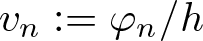 $v_n := \varphi_n/h$ satisfies, for
 $M \gt \widetilde{M}_1$,
 \begin{equation}
\begin{cases}
(\mathcal{L_{I}}_{hn} + M)v_n = (\sigma_n + M)v_n & \text{ in } \Omega, \\
\mathfrak{B}_h v_n = 0 & \text{ on } \partial\Omega,
\end{cases}
\end{equation}
where
 \begin{equation*}
\mathcal{L_I}_{hn}u := \mathcal{L}_h u - \int_{\Omega} K_{hn}(x, y) u(y) \, dy, \quad \text{and} \quad K_{hn}(x, y) := K_n(x, y) \frac{h(y)}{h(x)}.
\end{equation*}
Utilizing the argument presented in the proof of Lemma 2.2, there exists a constant  $M^* \gt 0$ (independent of n) such that the bilinear form
 $\mathfrak{b}_{hn}$ associated with (2.11) is coercive whenever
 $M \gt M^*$. Consequently, we fix
 $M \gt \max\{\widetilde{M}_1, M^*\}$.
Note that vn satisfies
 \begin{equation*}
\frac{\theta}{2}\|v_n\|^2_{W^{1,2}_{\Gamma_0}(\Omega)} \leq \mathfrak{b}_{hn}(v_n, v_n) = \sigma_n \|v_n\|^2_{L^2(\Omega)} \leq \sigma_1[\mathcal{L},\mathfrak{B},\Omega].
\end{equation*}
Hence, vn is bounded in  $W^{1,2}_{\Gamma_0}(\Omega)$, and therefore there exists
 $v^* \in W^{1,2}_{\Gamma_0}(\Omega)$ such that, along some subsequence relabeled by n,
 \begin{equation}
v_n \rightharpoonup v^* \text{ in } W^{1,2}_{\Gamma_0}(\Omega) \quad \text{and} \quad v_n \to v^* \text{ in } L^2(\Omega).
\end{equation}
Given that vn is a solution of (2.11), by definition, we have
 \begin{equation}
\mathfrak{b}_{hn}(v_n, \psi) = \sigma_n \int_\Omega v_n \psi, \quad \forall \psi \in C^{\infty}_{\Gamma_0}(\Omega).
\end{equation}
Combining (2.12) with the Dominated Convergence Theorem and letting  $n \to +\infty$ in (2.13) yields
 \begin{equation*}
\mathfrak{b}_{h}(v^*, \psi) = \sigma^* \int_\Omega v^* \psi, \quad \forall \psi \in C^{\infty}_{\Gamma_0}(\Omega).
\end{equation*}
Since  $v_n \geq 0$ and
 $\|v_n\|_{L^2(\Omega)} = 1$, it follows that
 $v^* \geq 0$ and
 $v^*\neq 0$. By Lemma 2.4,
 $v^*h \gt 0$ is the eigenfunction associated with
 $\sigma^*$ and, therefore,
 $\sigma^* = \sigma_1[\mathcal{L_I}, \mathfrak{B}, \Omega]$. This concludes the proof.
As a consequence of this proposition, we can obtain the following pointwise characterization of the principal eigenvalue.
Proposition 2.6.
Define the following set:
 \begin{equation*}\mathfrak P:=\left\{\psi\in W^{2,p}(\Omega),\,p \gt N;\psi(x) \gt 0,\,\forall x\in\Omega\quad\text{and}\quad\mathfrak B\psi\geq 0\ \text{on}\ \partial\Omega\right\}.\end{equation*}
Then,
 \begin{equation}
\sigma_1[\mathcal{L_{I}},\mathfrak{B},\Omega]=\sup_{\psi\in\mathfrak{P}}\inf_{x\in\Omega}\frac{\mathcal{L_{I}}\psi}{\psi}.
\end{equation}
Proof. Fix  $\lambda \lt \sigma_0=\sigma_1[\mathcal{L_I},\mathfrak{B},\Omega]$. Then
 $\sigma_1[\mathcal{L_I}-\lambda,\mathfrak{B},\Omega] = \sigma_0-\lambda \gt 0$. By Theorem 2.8, there exists
 $w_1 \in C_\mathfrak{B}^1(\overline{\Omega}) \cap W^{2,p}(\Omega)$, p > N, a unique solution of
 \begin{equation*}\begin{cases}
(\mathcal{L_{I}}-\lambda)u=1&\text{ in }\Omega,\\
\mathfrak{B}u=0&\text{on }\partial\Omega.
\end{cases}
\end{equation*}
Moreover,  $w_1\gg0$, and therefore
 $\mathfrak{P}\neq\emptyset$. Thus, for every
 $\lambda \lt \sigma_0$, we have
 \begin{equation*}
\lambda\le\inf_{x\in\Omega}\frac{\mathcal{L_{I}}w_1(x)}{w_1(x)}\le\sup_{\psi\in\mathfrak{P}}\inf_{x\in\Omega}\frac{\mathcal{L_{I}}\psi(x)}{\psi(x)}.
\end{equation*}
Consequently,
 \begin{equation*}\sigma_0\le\sup_{\psi\in\mathfrak{P}}\inf_{x\in\Omega}\frac{\mathcal{L_{I}}\psi(x)}{\psi(x)}.\end{equation*}
Assume, by contradiction, that the above inequality is strict. Then there exist ϵ > 0 and  $w_2\in\mathfrak{P}$ such that
 \begin{equation*}\sigma_0+\epsilon \lt \frac{\mathcal{L_I }w_2}{w_2} \quad\text{ in }\Omega.\end{equation*}
Therefore w 2 is a positive strict supersolution of  $(\mathcal{L_I}-\sigma_0-\epsilon,\mathfrak{B},\Omega)$. By Theorem 2.8, we have
 \begin{equation*}0 \lt \sigma_1[\mathcal{L_I}-\sigma_0-\epsilon,\mathfrak{B},\Omega]=-\epsilon,\end{equation*}
which is a contradiction.
We conclude this section by establishing the concavity of the mapping
 \begin{equation*}P \in L^{\infty}(\Omega) \longmapsto \sigma(P):=\sigma_1[\mathcal{L_I}+P,\mathfrak{B},\Omega].\end{equation*}
Proposition 2.7.
For all  $P_1, P_2\in L^{\infty}(\Omega)$ and
 $t\in [0,1],$ it holds that
 \begin{equation*}\sigma(tP_1+(1-t)P_2)\ge t\sigma (P_1)+(1-t)\sigma (P_2).\end{equation*}
Proof. Consider the function  $G: W^{2,p}(\Omega)\rightarrow C(\overline{\Omega})$, p > N, given by
 \begin{equation*}G(u)=(\mathcal{L}-c)u+c+R(u),\end{equation*}
where  $R(u):=-\sum_{i,j=1}^{N}a_{ij}\partial_i u\partial_j u$. By the proof of [Reference López-Gómez22, Th. 8.3], we have that G is a concave function and satisfies
 \begin{equation*}G(\log \psi)=\frac{\mathcal{L}\psi}{\psi},\end{equation*}
for all  $\psi\in \mathfrak{P}$. Now define
 $H:W^{2,p}(\Omega)\rightarrow C(\overline{\Omega})$,
 $p \gt N,$ given by
 \begin{equation*}H(u)=-\int_{\Omega} K(x,y)e^{u(y)-u(x)}dy.\end{equation*}
Let us show that H is concave. Indeed, for each  $x,y\in \Omega$,
 $u_1,u_2\in W^{2,p}(\Omega)$,
 $p \gt N,$ we have
 \begin{equation*}\begin{array}{ll}
H(tu_1+(1-t)u_2)&=-\int_{\Omega} K(x,y)e^{t(u_1(y)+u_1(x))+(1-t)(u_2(y)-u_2(x))}dy\\
&\ge -\int_{\Omega} K(x,y)\left[te^{u_1(y)+u_1(x)}+(1-t)e^{u_2(y)-u_2(x)}\right]dy\\
&=t H(u_1)+(1-t)H(u_2).
\end{array}\end{equation*}
Since both G and H are concave, it follows that  $G_{\mathcal{I}}(u):=G(u)+H(u)$ is also concave. Furthermore, for all
 $\psi\in \mathfrak{P}$, we have
 \begin{equation*}
G_\mathcal{I}(\log\psi)=G(\log\psi)+H(\log\psi) =\frac{\mathcal{L}\psi}{\psi}-\int_{\Omega} K(x,y)\frac{\psi(y)}{\psi(x)}dy =\frac{\mathcal{L_I}\psi}{\psi}.
\end{equation*}
Now let  $\psi_1,\psi_2\in \mathfrak{P}$,
 $P_1,P_2\in L^{\infty}(\Omega)$. Since
 $\phi\in\mathfrak{P}$, it follows that
 $1/\phi\in L^{\infty}(\Omega)$ and
 $\nabla\phi\in L^{\infty}(\Omega,\mathbb{R}^N)$. Consequently,
 $\psi_1^t\psi_2^{1-t}\in \mathfrak{P}$. Therefore,
 \begin{equation*}\begin{array}{ll}
\frac{[\mathcal{L_I}+tP_1+(1-t)P_2](\psi_1^t\psi_2^{1-t})}{\psi_1^t\psi_2^{1-t}}
&=tP_1+(1-t)P_2+G_\mathcal{I}(\log(\psi_1^t\psi_2^{1-t}))\\
&\ge tP_1+(1-t)P_2+tG_\mathcal{I}(\log(\psi_1))+(1-t)G_\mathcal{I}(\log(\psi_2))\\
&=t\frac{(\mathcal{L_I}+P_1)\psi_1}{\psi_1}+(1-t)\frac{(\mathcal{L_I}+P_2)\psi_2}{\psi_2}.
\end{array}\end{equation*}
Since this last inequality holds for any  $\psi_1,\psi_2\in\mathfrak{P}$ and in view of (2.14), we obtain the result.
3. Eigenvalue problem with indefinite weight
Throughout this section, we will assume Hypothesis (b 1), and the main goal is to establish sufficient conditions for the existence of a principal eigenvalue for the following problem:
 \begin{equation}
\left\{
\begin{array}{ll}
\mathcal{L_I}_0u:= \mathcal{L}u-\displaystyle\int_{\Omega_0}K(x,y)u(y)dy=\lambda m(x)u & \text{ in } \Omega_0,\\
\mathfrak{B}_{0}u=0 & \text{ on } \partial \Omega_0,
\end{array}\right.
\end{equation}
where  $\mathfrak{B}_0:=\mathfrak{B}[\Omega_{0}]$, which is well-defined, by (b 1).
Furthermore, we will show that, when it exists, it can be approximated by the following auxiliary eigenvalue problem:
 \begin{equation}\left\{\begin{array}{lc}{\mathcal L}_{\mathcal I}u+\mu b(x)u=\lambda m(x)u&\text{in}\ \Omega,\\\mathfrak Bu=0&\ \text{on}\ \partial\Omega,\end{array}\right.\end{equation}
when  $\mu \to +\infty$.
In this section, we will use assumptions (b 1), (m 1) and the following additional condition:
(Λ0) There exists
$\lambda_0 \in \mathbb{R}$ such that
\begin{equation*}
\sigma_1[\mathcal{L_I}_0-\lambda_0 m, \mathfrak{B}_0, \Omega_0] \gt 0.
\end{equation*}


We emphasize that this section substantially generalizes the results of [Reference Wan-Tong, López-Gómez and Sun28,  $\S$ 3]
3.1. The eigenvalue with indefinite weight
In this section, we establish the existence of the principal eigenvalue for problem (E 0). To this end, we define
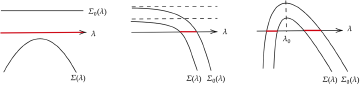
 \begin{equation*}\Sigma_0(\lambda):=\sigma_1[\mathcal{L_{I}}_0-\lambda m,\mathfrak{B}_0,\Omega_0],\quad \lambda \in\mathbb{R}.\end{equation*}
Note that  $\lambda \in \mathbb{R}$ is a principal eigenvalue of (E 0) if, and only if,
 $\Sigma_0(\lambda)=0.$
Using the properties of the principal eigenvalue derived in the previous section, we obtain the following result:
Proposition 3.1.
The mapping  $\Sigma_0(\lambda)$ is real analytic and concave. Moreover, the following holds:
(i) if there exists  $x_+\in \Omega_0$ such that
 $ m(x_+) \gt 0$, then
 \begin{equation*}
\lim_{\lambda\to +\infty}\Sigma_0(\lambda)=-\infty;
\end{equation*}
(ii) if there exists  $x_-\in \Omega_0$ such that
 $m(x_-) \lt 0$, then
 \begin{equation*}
\lim_{\lambda\to -\infty}\Sigma_0(\lambda)=-\infty.
\end{equation*}
Proof. To establish that  $\Sigma_0(\lambda)$ is real analytic, we consider the family of operators
 $\mathcal{T}(\lambda): W^{2,p}(\Omega_0)\rightarrow L^2(\Omega_0)$ given by
 \begin{equation*}
\mathcal{T}(\lambda)u:=\mathcal{L_I}u-\lambda m u.
\end{equation*}
For each  $u\in W^{2,p}(\Omega_0)$, p > N, and
 $v\in L^2(\Omega_0)$, the mapping
 $ \lambda \in \mathbb{R} \mapsto \langle v,\mathcal{L_I}(\lambda)u\rangle_{L^2(\Omega_0)} $ is real analytic. Hence,
 $\mathcal{T}(\lambda)$ is a real holomorphic family of type (A), as described in [Reference Kato21]. Consequently, Theorems 1.7 and 1.8 of [Reference Kato21,
 $\S$ VII.1.3] imply that
 $ \Sigma_0(\lambda) $ is real analytic.
The concavity of  $\Sigma_0(\lambda)$ follows directly from Proposition 2.7.
To prove (i), note that the continuity of m ensures the existence of  $r_1 \gt 0$ such that
 $\inf_{B} m \gt 0$, where
 $B:=B_{r_1}(x_+)$ is such that
 $\overline{B} \subset \Omega_0$. Using Proposition 2.5 (ii), we conclude that
 \begin{equation*}\begin{array}{ll}
\Sigma_0(\lambda) & \lt \sigma_1[\mathcal{L} - \int_{B}K(x,y) \cdot dy-\lambda m,\mathfrak{D},B] \\
& \lt \sigma_1[\mathcal{L}- \int_{B}K(x,y) \cdot dy,\mathfrak{D},B]-\lambda \inf_{B} m.
\end{array}\end{equation*}
Letting  $\lambda \to +\infty$ in the above inequality yields the desired result. The proof of (ii) follows similarly by considering a point
 $x_-\in\Omega_0$, where
 $m(x_-) \lt 0$.
Remark 3.1. An analogous result holds for the eigenvalue  $\sigma_1[\mathcal{L_I}-\lambda m,\mathfrak{B},\Omega]$.
This result provides sufficient conditions to guarantee the existence of a principal eigenvalue for problem (E 0). Indeed, the following theorem holds:
Theorem 3.2 Suppose (b1), (m1), and (Λ0) hold. Then, problem (E0) has a unique principal eigenvalue, denoted by  $\lambda_1^{\mathfrak B_0}(\Omega_0),$ such that
 \begin{equation*}\lambda_0 \lt \lambda_1^{\mathfrak B_0}(\Omega_0).\end{equation*}
Proof. By assumption (m 1) and using Proposition 3.1 (i), we have
 \begin{equation*}
\lim_{\lambda\to +\infty}\Sigma_0(\lambda)=-\infty.
\end{equation*}
On the other hand, by hypothesis (Λ 0), we get  $\Sigma_0(\lambda_0) \gt 0$. Since
 $\Sigma_0\neq 0$ is real analytic and concave to ensure that there exists a unique
 $\lambda_1^{\mathfrak B_0}(\Omega_0) \gt \lambda_0$,
 $\Sigma_0(\lambda_1^{\mathfrak B_0}(\Omega_0))=0$.
3.2. Approximated eigenvalues
We now establish that the principal eigenvalue of problem (Eλ,μ) converges to the principal eigenvalue of problem (E 0), when it exists.
To this end, we define the mappings
 \begin{align}
\Sigma(\lambda)&:=\sigma_1[\mathcal{L_{I}}-\lambda m,\mathfrak{B},\Omega],\nonumber\\
\Sigma(\lambda,\mu)&:=\sigma_1[\mathcal{L_{I}}-\lambda m+\mu b,\mathfrak{B},\Omega],\nonumber\\
\Sigma_0(\lambda)&:=\sigma_1[\mathcal{L_{I}}_0-\lambda m,\mathfrak{B}_0,\Omega_0],
\end{align}
where  $\lambda,\mu\in\mathbb R$, and
 $\mu\geq0$. Additionally, we assume that
 \begin{equation*}a_{ij}\in C^1(\overline\Omega)\ \text{and}\ b_j\in C(\overline\Omega),\quad 1\leq i,j\leq N.\end{equation*}
Under these assumptions, the following result holds:
Theorem 3.3 Assume (b1). The mappings defined in (3.1) are real analytic and concave with respect to the parameter λ. Moreover, the mapping
 \begin{equation*}\mu\in [0,+\infty)\mapsto \Sigma(\cdot,\mu)\in C(\mathbb R),\end{equation*}
is strictly increasing and satisfies
 \begin{equation}
\Sigma(\lambda) \lt \Sigma(\lambda,\mu) \lt \Sigma_0(\lambda),\quad\forall \lambda\in\mathbb R, \, \mu \gt 0.
\end{equation}
Furthermore,  $\Sigma(\lambda,0)=\Sigma(\lambda)$, and for each
 $\lambda\in \mathbb{R}$,
 \begin{equation}
\lim_{\mu \to +\infty}\Sigma(\lambda,\mu)=\Sigma_0(\lambda).
\end{equation}
Proof. By Proposition 3.1, the mappings defined in (3.1) are real analytic and concave. Since  $b\geq0$, Proposition 2.5 (iii) ensures that the mapping
 $\mu\in[0,+\infty)\mapsto\Sigma(\cdot,\mu)$ is strictly increasing. Thus,
 \begin{equation}
\Sigma(\lambda)=\Sigma(\lambda,0)=\sigma_1[\mathcal{L_{I}}-\lambda m,\mathfrak{B},\Omega] \lt \sigma_1[\mathcal{L_{I}}-\lambda m+\mu b,\mathfrak{B},\Omega]=\Sigma(\lambda,\mu).
\end{equation}
Using Proposition 2.5 (ii), we also obtain
 \begin{equation}
\Sigma(\lambda,\mu)=\sigma_1[\mathcal{L_{I}}-\lambda m+\mu b,\mathfrak{B},\Omega] \lt \sigma_1[\mathcal{L_{I}}_0-\lambda m,\mathfrak{B}_0,\Omega_0]=\Sigma_0(\lambda),
\end{equation}
for all  $\lambda\in\mathbb R, \mu\geq0$. Combining (3.4) and (3.5) gives (3.2). Finally, (3.3) follows directly from [Reference López-Gómez22, Th. 9.6].
Let us consider the case where a positive principal eigenvalue exists for problem (E 0), which, as we will see, guarantees the existence of the principal eigenvalue of (Eλ,μ), for sufficiently large µ.
Corollary 3.4. Assume (b1), (m1), and (Λ0). Then, there exists  $\bar\mu\in\mathbb R$ such that, for all
 $\mu \gt \bar\mu$, problem (Eλ,μ) admits a unique principal eigenvalue, denoted by
 $\lambda_1^{\mathfrak B}(\mu,\Omega),$ which satisfies
 \begin{equation*}
\lambda_0 \lt \lambda_1^{\mathfrak B}(\mu,\Omega) \lt \lambda_1^{\mathfrak {B}_0}(\Omega_0).
\end{equation*}
Moreover, the mapping
 \begin{equation*}
\mu\in(\bar\mu,+\infty)\mapsto \lambda_1^{\mathfrak B}(\mu,\Omega)\in (\lambda_0,\lambda_1^{\mathfrak {B}_0}(\Omega_0)),
\end{equation*}
is strictly increasing and continuous and satisfies
 \begin{equation}
\lim_{\mu\uparrow\infty}\lambda_1^{\mathfrak{B}}(\mu,\Omega)=\lambda_1^{\mathfrak{B}_0}(\Omega_0).
\end{equation}
Proof. By hypothesis (Λ 0) and equation (3.3), there exists  $\bar\mu \gt 0$, such that
 $\Sigma(\lambda_0,\mu) \gt 0$, for all
 $\mu\ge\bar\mu$. By hypothesis (m 1) and Proposition 3.1 (ii), for each
 $\mu \ge \bar \mu$, we have
 \begin{equation*}
\lim_{\lambda \to +\infty} \Sigma(\lambda,\mu) =-\infty.
\end{equation*}
Thus, for a fixed  $\mu \ge\bar \mu$, the monotonicity properties of the continuous mapping
 $\lambda \mapsto \Sigma(\lambda,\mu)$, guarantee the existence of a unique
 $\lambda_1^{\mathfrak B}(\mu,\Omega) \gt \lambda_0$, such that
 \begin{equation*}
\Sigma(\lambda_1^{\mathfrak B}(\mu,\Omega), \mu)=0.
\end{equation*}
Hence,  $\lambda_1^{\mathfrak B}(\mu,\Omega)$ is an principal eigenvalue of (Eλ,μ).
Next, we prove that the mapping  $\mu \in [\bar\mu,+\infty)\mapsto \lambda_1^{\mathfrak B}(\mu,\Omega)$ is strictly increasing. Consider
 $\bar\mu\le\mu_1 \lt \mu_2.$ Then, there exist unique real numbers
 $\lambda_1^{\mathfrak B}(\mu_1,\Omega)$ and
 $\lambda_1^{\mathfrak B}(\mu_2,\Omega)$ both greater than
 $\lambda_0,$ such that
 \begin{equation*}\Sigma(\lambda_1^{\mathfrak B}(\mu_1,\Omega),\mu_1)=0 \quad\text{and}\quad\Sigma(\lambda_1^{\mathfrak B}(\mu_2,\Omega),\mu_2)=0.\end{equation*}
Since the mapping  $\mu\mapsto\Sigma(\lambda,\mu)$ is increasing for all
 $\lambda\in\mathbb R$, we have
 \begin{equation*}
\Sigma(\lambda_1^{\mathfrak B}(\mu_1,\Omega),\mu_2) \gt \Sigma(\lambda_1^{\mathfrak B}(\mu_1,\Omega),\mu_1)=0.
\end{equation*}
Arguing as in the proof of Theorem 3.2, there exists a unique  $\lambda^* \gt \lambda_1^{\mathfrak B}(\mu_1,\Omega)$ such that
 $\Sigma(\lambda^*,\mu_2)=0.$ By uniqueness, we must have
 $\lambda^*=\lambda_1^{\mathfrak B}(\mu_2,\Omega).$ This proves that
 $\lambda_1^\mathfrak{B}(\mu,\Omega)$ is strictly increasing with respect to µ.
To prove continuity, let  $\{\mu_n\}_{n\geq1}$ be an increasing sequence such that
 $\mu_n\to\mu^*$, with
 $\bar\mu\le\mu_n,$ for all
 $n\in\mathbb{N}$. By Proposition 2.5 (ii), we have
 \begin{equation*}
\Sigma(\lambda,\mu) \lt \Sigma_0(\lambda),\quad\forall\mu\geq0,
\end{equation*}
which implies that
 \begin{equation}
\lambda_1^{\mathfrak{B}}(\mu,\Omega) \lt \lambda_1^{\mathfrak{B}_0}(\Omega_0),\quad\forall \mu\geq0.
\end{equation}
Therefore,  $\left\{\lambda_1^{\mathfrak{B}}(\mu_n,\Omega)\right\}_{n\geq1}$ is an increasing and bounded sequence, which implies the existence of
 $\bar{\lambda} \in \mathbb{R}$ such that
 \begin{equation*}
\lim_{n\to\infty}\lambda_1^{\mathfrak{B}}(\mu_n,\Omega) = \bar{\lambda}.
\end{equation*}
Moreover, for each  $n \in \mathbb{N}$,
 \begin{equation*}
\Sigma(\lambda_1^{\mathfrak{B}}(\mu_n,\Omega), \mu_n) = 0.
\end{equation*}
By the continuity of  $(\lambda, \mu) \mapsto \Sigma(\lambda, \mu) $,
 \begin{equation*}
0 = \lim_{n\to\infty}\Sigma(\lambda_1^{\mathfrak{B}}(\mu_n,\Omega), \mu_n) = \Sigma\left(\lim_{n\to\infty}\lambda_1^{\mathfrak{B}}(\mu_n,\Omega), \lim_{n\to\infty}\mu_n\right) = \Sigma(\bar{\lambda}, \mu^*).
\end{equation*}
By arguments similar to those in Theorem 3.2, the map  $\lambda \in (\lambda_0,+\infty) \mapsto \Sigma(\lambda, \mu^*)$ has a unique zero. Therefore, we must have
 $\bar{\lambda} = \lambda_1^{\mathfrak{B}}(\mu^*, \Omega)$.
Finally, we prove (3.6). From (3.7), it follows that  $\lambda_1^{\mathfrak{B}}(\mu, \Omega)$ is bounded for all
 $\mu \geq \bar\mu$. Since
 $\lambda_1^\mathfrak{B}(\mu,\Omega)$ is strictly increasing with respect to µ, we can define
 \begin{equation*}
\lambda_0 \lt \lambda_{\infty} := \lim_{\mu\to\infty}\lambda_1^{\mathfrak{B}}(\mu, \Omega).
\end{equation*}
Consequently, for any ϵ > 0, there exists  $\mu(\epsilon) \geq \bar\mu$ such that
 \begin{equation*}
-\lambda_\infty m(x) - \epsilon \le -\lambda_1^{\mathfrak{B}}(\mu, \Omega)m(x) \le -\lambda_\infty m(x) + \epsilon,
\end{equation*}
for all  $\mu \ge \mu(\epsilon)$. By Proposition 2.5 (iii), for
 $\mu \ge \mu(\epsilon)$, we have
 \begin{equation*}\begin{array}{ll}
\sigma_1[\mathcal{L_{I}} - \lambda_\infty m(x) + \mu b(x), \mathfrak{B}, \Omega] - \epsilon &\le \sigma_1[\mathcal{L_{I}} - \lambda_1^{\mathfrak{B}}(\mu, \Omega)m(x) + \mu b(x), \mathfrak{B}, \Omega] \\
& \lt \sigma_1[\mathcal{L_{I}}_0 - \lambda_1^{\mathfrak{B}}(\mu, \Omega)m(x), \mathfrak{B}_0, \Omega_0].
\end{array}\end{equation*}
Letting  $\mu\to\infty$ in the above inequalities and applying [Reference López-Gómez22, Th. 9.6], along with the continuity of the principal eigenvalue with respect to the potential, we obtain that, for every ϵ > 0,
 \begin{equation*}\begin{array}{ll}
\sigma_1[\mathcal{L_{I}}_0-\lambda_\infty m(x),\mathfrak{B}_0,\Omega_0]-\epsilon&\le\lim_{\mu\to\infty}\sigma_1[\mathcal{L_{I}}-\lambda_1^{\mathfrak{B}}(\mu,\Omega)m(x)+\mu b(x),\mathfrak{B},\Omega]\\
&\le\sigma_1[\mathcal{L_{I}}_0-\lambda_\infty m(x),\mathfrak{B}_0,\Omega_0].
\end{array}\end{equation*}
Letting  $\epsilon\to 0^+$ yields
 \begin{equation*}\lim_{\mu\to\infty}\sigma_1[\mathcal{L_{I}}-\lambda_1^{\mathfrak{B}}(\mu,\Omega)m(x)+\mu b(x),\mathfrak{B},\Omega] =\sigma_1[\mathcal{L_{I}}_0-\lambda_\infty m(x),\mathfrak{B}_0,\Omega_0].\end{equation*}
On the other hand, for any  $\mu\geq\bar\mu$, we have
 \begin{equation*}
0=\Sigma(\lambda_1^{\mathfrak{B}}(\mu,\Omega),\mu)=\sigma_1[\mathcal{L_{I}}-\lambda_1^{\mathfrak{B}}(\mu,\Omega)m(x)+\mu b(x),\mathfrak{B},\Omega],
\end{equation*}
and thus
 \begin{equation*}\begin{array}{ll}
0=\lim_{\mu\to\infty}\Sigma(\lambda_1^{\mathfrak{B}}(\mu,\Omega),\mu)&=\lim_{\mu\to\infty}\sigma_1[\mathcal{L_{I}}-\lambda_1^{\mathfrak{B}}(\mu,\Omega)m(x)+\mu b(x),\mathfrak{B},\Omega]\\
&=\sigma_1[\mathcal{L_{I}}_0-\lambda_\infty m(x),\mathfrak{B}_0,\Omega_0]\\
&=\Sigma_0(\lambda_{\infty}).
\end{array}\end{equation*}
By the uniqueness of the zero of the mapping  $\lambda\in (\lambda_0,+\infty)\mapsto\Sigma_0(\lambda)$, we conclude that
 \begin{equation*}\lambda_{\infty}=\lambda_1^{\mathfrak{B}_0}(\Omega_0).\end{equation*}
A particularly interesting case arises when the following condition is satisfied:
(Λ′0) There exists
$\lambda_0 \in \mathbb{R}$ such that
\begin{equation*}
\sigma_1[\mathcal{L_I}-\lambda_0 m, \mathfrak{B}, \Omega] \gt 0.
\end{equation*}


Since  $\Sigma(\lambda) \lt \Sigma_0(\lambda)$, (Λ′0) implies (Λ0). In this case, we have the following result:
Corollary 3.5. Assume (b1), (m1), and (Λ′0). Then, for each µ > 0, problem (Eλ,μ) admits a unique principal eigenvalue, denoted by  $\lambda_1^{\mathfrak{B}}(\mu,\Omega)$, which satisfies
 \begin{equation}
\lambda_1^{\mathfrak{B}}(\Omega) \lt \lambda_1^{\mathfrak{B}}(\mu,\Omega) \lt \lambda_1^{\mathfrak{B}_0}(\Omega_0).
\end{equation}
Moreover, the mapping
 \begin{equation*}
\mu\in(0,+\infty)\mapsto \lambda_1^{\mathfrak B}(\mu,\Omega)\in (\lambda_1^{\mathfrak{B}}(\Omega),\lambda_1^{\mathfrak {B}_0}(\Omega_0))
\end{equation*}
is strictly increasing and continuous and satisfies
 \begin{equation}
\lim_{\mu\uparrow\infty}\lambda_1^{\mathfrak{B}}(\mu,\Omega)=\lambda_1^{\mathfrak{B}_0}(\Omega_0).
\end{equation}
Proof. Since  $\Sigma(\lambda,0)=\Sigma(\lambda)$, the mapping
 $\mu\mapsto\Sigma(\lambda,\mu)$ is strictly increasing, and (Λ′0) is satisfied, we obtain (3.8). The remaining assertions follow from the previous corollary.
Finally, we show that under the general conditions, the principal eigenfunctions of (Eλ,μ) also converge to the principal eigenfunctions of (E 0).
Theorem 3.6 Assume (b1), (m1), and (Λ0). For each  $\mu\ge\bar\mu$, let
 $\varphi_\mu \gt 0$ and
 $\varphi_{0} \gt 0$ be the eigenfunctions associated with
 $\lambda_1^{\mathfrak{B}}(\mu,\Omega)$ and
 $\lambda_1^{\mathfrak{B}_{0}}(\Omega_0)$, respectively, normalized such that
 \begin{equation*}
\int_{\Omega}\varphi_\mu^2=\int_{\Omega_0}\varphi_{0}^2=1.
\end{equation*}
Then
 \begin{equation}
\lim_{\mu\to\infty}\|\varphi_\mu-\psi\|_{{}_{W^{1,2}(\Omega)}}=0,
\end{equation}
where
 \begin{equation*}
\psi=\left\{
\begin{array}{ll}
\varphi_{0} &\text{ in }\overline{\Omega}_0,\\
0&\text{ in }\Omega\setminus\overline{\Omega}_0.
\end{array}\right.
\end{equation*}
Moreover, there exists a constant  $r=r(N)\ge1$, such that whenever
 $a_{ij}\in C^{r,1}(\overline{\Omega}_0), b_j, c, m\in C^{r-1,1}(\overline{\Omega}_0)$, and for each
 $y\in\Omega_0$, the mapping
 $x\mapsto K(x,y)$ is of class
 $ C^{r-1,1}(\overline{\Omega}_0)$, then
 \begin{equation}
\lim_{\mu\to\infty}\varphi_\mu=\psi, \text{\quad uniformly on compact subsets of }\Omega_0.
\end{equation}
Proof. Consider, for all  $ u,v \in W^{1,2}_{\Gamma_0}(\Omega) $, the bilinear form associated with the operator
 $ \mathcal{L_I} $:
 \begin{equation}
\mathfrak{b}(u,v)=\int_{\Omega}\langle A\nabla u,\nabla v\rangle+\int_{\Omega}\left(\langle \vec b, \nabla u\rangle +uc\right)v+\int_{\Gamma_1}\beta uv dS-\int_{\Omega}\int_{\Omega}vK(x,y)u(y)dy,
\end{equation}
and we define
 \begin{equation*} \mathfrak{b^+}(u,v):=\mathfrak{b}(u,v)+\int_{\Gamma_1}\beta^-uvdS, \end{equation*}
where  $ \beta^-(x):=\max\{-\beta(x),0\} $. By Lemma 2.2, for M > 0 sufficiently large, we find that
 \begin{equation*} \mathfrak{b}^+_M(u,v):=\mathfrak{b}^+(u,v)+M\int_\Omega uv \end{equation*}
is coercive. To simplify the notation, let us denote  $ \lambda_\mu=\lambda^{\mathfrak{B}}_1(\mu,\Omega) $. Thus, φµ satisfies
 \begin{equation*} (\mathcal{L_{I}}+M)\varphi_\mu+\mu b\varphi_\mu=\lambda_\mu\varphi_\mu +M\varphi_\mu \quad \text{in } \Omega. \end{equation*}
Multiplying this equation by φµ, integrating over Ω, and applying the integration by parts, we obtain
 \begin{equation}
\mathfrak{b}^+_M(\varphi_\mu,\varphi_\mu)=\lambda_\mu \int_\Omega m\varphi^2_\mu+M\int_\Omega\varphi^2_\mu+\int_{\Gamma_1}\beta^-\varphi_\mu^2-\mu \int_\Omega b\varphi^2_\mu.
\end{equation}
Since  $ b_M^+ $ is coercive, there exists a constant
 $ C_0 \gt 0 $ such that
 \begin{align*}\begin{array}{lc}C_0\Arrowvert\varphi_\mu\Arrowvert_{W_{\Gamma_0}^{1,2}(\Omega)}^2&\leq\lambda_\mu\int_\Omega m\varphi_\mu^2+M\int_\Omega\varphi_\mu^2+\int_{\Gamma_1}\beta^-\varphi_\mu^2-\mu\int_\Omega b\varphi_\mu^2\\&\leq\lambda_\infty\Arrowvert m\Arrowvert_{L^\infty(\Omega)}+M+\Arrowvert\beta\Arrowvert_{L^\infty(\partial\Omega)}\int_{\Gamma_1}\varphi_\mu^2.\end{array}\end{align*}
By [Reference Afrouzi and Brown2, Lemma 1], for each ϵ > 0, there exists  $ C(\epsilon) \gt 0 $ such that
 \begin{equation*}\begin{array}{ll}
\int_{\Gamma_1}\varphi_\mu^2 &\le \int_{\partial\Omega}\varphi_\mu^2 \le \epsilon\int_{\Omega}|\nabla\varphi_\mu|^2+C(\epsilon)\int_{\Omega}\varphi_\mu^2\\
&\le \epsilon\left(\int_{\Omega}|\nabla\varphi_\mu|^2+\int_{\Omega}\varphi_\mu^2\right)+C(\epsilon).
\end{array}\end{equation*}
Thus,
 \begin{equation*}
C_0\|\varphi_\mu\|^2_{W^{1,2}_{\Gamma_{0}}(\Omega)} \le \lambda_{\infty}\|m\|_{L^\infty(\Omega)}+M+\|\beta\|_{L^\infty(\partial\Omega)}\left(\epsilon\|\varphi_\mu\|^2_{W^{1,2}_{\Gamma_{0}}(\Omega)}+C(\epsilon)\right).
\end{equation*}
Choosing ϵ > 0 sufficiently small such that  $ \|\beta\|_{L^\infty(\partial\Omega)}\epsilon \lt C_0 $, we have
 \begin{equation*}
\|\varphi_\mu\|^2_{W^{1,2}_{\Gamma_{0}}(\Omega)} \le \sqrt{\frac{\lambda_{\infty}\|m\|_{L^\infty(\Omega)}+M+\|\beta\|_{L^\infty(\partial\Omega)}C(\epsilon)}{C_0-\epsilon\|\beta\|_{L^\infty(\partial\Omega)}}} =:\tilde{C}.
\end{equation*}
Thus,  $ \{\varphi_\mu\}_\mu $ is bounded in
 $ W^{1,2}_{\Gamma_{0}}(\Omega)$. Therefore, for any increasing sequence
 $ \{\mu_n\}_n $ such that
 $ \lim_{n \to \infty} \mu_n =\infty $, we can extract a subsequence, relabelled by n, and a function
 $ \psi\in W^{1,2}_{\Gamma_{0}}(\Omega) $, such that
 \begin{equation*}
\varphi_{\mu_n}\rightharpoonup\psi\text{ in } W^{1,2}_{\Gamma_{0}}(\Omega) \quad \mbox{and} \quad \varphi_{\mu_n}\to\psi\text{ in } L^{2}(\Omega).
\end{equation*}
For simplicity, let
 \begin{equation*}\varphi_n:=\varphi_{\mu_n}\ \text{and}\ \lambda_n:=\lambda_{\mu_n}.\end{equation*}
On the other hand, it follows from (3.13) that
 \begin{equation*}\begin{array}{ll}
\mu_n \int_\Omega b\varphi^2_n &= \lambda_n\int_\Omega\varphi^2_{n}-\mathfrak{b}^+_M(u,v)+M\int_\Omega \varphi^2_{n}+\int_{\Gamma_1}\beta^-\varphi_{n}^2\\
&\le \lambda_\infty m\int_\Omega\varphi^2_{n}+M\int_\Omega\varphi^2_{n}+\int_{\Gamma_1}\beta^-\varphi_{n}^2\\
&\le\lambda_{\infty}\|m\|_{L^\infty(\Omega)}+M+\|\beta^-\|_{L^\infty(\Omega)}\left( \epsilon\|\varphi_{n}\|^2_{W^{1,2}_{\Gamma_{0}}(\Omega)}+C(\epsilon)\right)\\
&\le\lambda_{\infty}\|m\|_{L^\infty(\Omega)}+M+\|\beta^-\|_{L^\infty(\Omega)}\left( \epsilon \tilde{C}+C(\epsilon)\right) \lt +\infty.
\end{array}\end{equation*}
Consequently,
 \begin{equation*}
\lim_{n\to\infty}\int_{\Omega\setminus\overline{\Omega}_0}b\varphi^2_n=0.
\end{equation*}
Since  $ \{\varphi_{n}\}_n $ converges in
 $ L^2(\Omega) $, the above limit implies that ψ = 0 on
 $ \Omega\setminus\ \overline{\Omega}_{0} $. In particular, by [Reference Cano-Casanova and López-Gómez8, Th. 6.4], we conclude that
 $ \psi \in W_{\partial \Omega_0 \cap \Omega}^{1,2}(\Omega_0) $.
Now, we show that
 \begin{equation*}
\lim_{n\to\infty}\|\varphi_{n} -\psi\|_{W^{1,2}_{\Gamma_{0}}(\Omega)}=0.
\end{equation*}
Since φn is an eigenfunction associated with  $ \lambda_n = \lambda_1^{\mathfrak{B}}(\mu_n,\Omega) $, we obtain
 \begin{align*}
&\mathfrak{b}(\varphi_n,\varphi_n)-2\mathfrak{b}(\varphi_n,\varphi_k)+\mathfrak{b}(\varphi_k,\varphi_k)\\
&\quad=\lambda_n\int_{\Omega}m(\varphi_n-\varphi_k)^2+(\lambda_k-\lambda_n)\int_{\Omega}m\varphi_k^2+(\mu_n-\mu_k)\int_{\Omega}b\varphi_k^2.
\end{align*}
Thus, since  $ \{\varphi_n\}_n $ and
 $ \{\lambda_n\}_n $ are Cauchy sequences, given ϵ > 0, there exists
 $ n_0\in \mathbb{N} $ such that
 \begin{align}
&\mathfrak{b}(\varphi_n,\varphi_n-\varphi_k)+\mathfrak{b}(\varphi_k-\varphi_n,\varphi_k)\nonumber\\
&\quad=\lambda_n\int_{\Omega}m(\varphi_n-\varphi_k)^2+(\lambda_k-\lambda_n)\int_{\Omega}m\varphi_k^2\nonumber\\
&\qquad+(\mu_n-\mu_k)\int_{\Omega}b\varphi_k^2\nonumber\\
&\quad\le\lambda_n\int_{\Omega}m(\varphi_n-\varphi_k)^2+(\lambda_k-\lambda_n)\int_{\Omega}m\varphi_k^2 \lt \epsilon,
\end{align}
whenever  $ n,k\ge n_0 $. On the other hand. using the definition of the bilinear form (3.12), we have
 \begin{align}
&\mathfrak{b}(\varphi_n,\varphi_n-\varphi_k)+\mathfrak{b}(\varphi_k-\varphi_n,\varphi_k)\nonumber\\
&\quad=\int_{\Omega}\langle A\nabla (\varphi_n-\varphi_k),\nabla (\varphi_n-\varphi_k)\rangle+\int_{\Omega}\langle \vec b, \nabla \varphi_n\rangle(\varphi_n-\varphi_k)\nonumber\\
&\qquad+\int_{\Omega}\langle \vec b,\nabla(\varphi_k-\varphi_n)\rangle\varphi_n + \int_{\Omega}c(\varphi_n-\varphi_k)^2\nonumber\\
&\qquad+\int_{\Gamma_1}\beta (\varphi_n-\varphi_k)^2 dS-\int_{\Omega}\int_{\Omega}(\varphi_n-\varphi_k) K(x,y)\varphi_n(y)dy\nonumber\\
&\qquad-\int_{\Omega}\int_{\Omega}\varphi_k K(x,y)(\varphi_k-\varphi_n)(y)dy.
\end{align}
Next, note that
 \begin{align}
\!\!\!\!\!\!\!\!\!\!\!\!\!\!\!\!\!\!\!\!\!\!\!\!\!\!\!\!\!\!\!\!\!\!\!\!\!\!\!\!\!\!\!\!\!\!\!\!\!\!\!\!\theta\|\varphi_n-\varphi_k\|_{W_{\Gamma_{0}}^{1,2}(\Omega)}\le\int_{\Omega}\langle A\nabla (\varphi_n-\varphi_k),\nabla (\varphi_n-\varphi_k)\rangle;
\end{align}
 \begin{align}
\int_{\Omega}\langle \vec b,\nabla(\varphi_k-\varphi_n)\rangle\varphi_n&\le\|\vec b\|_{L^{\infty}(\Omega)}\int_{\Omega}|\nabla(\varphi_k-\varphi_n)||\varphi_k|\nonumber\\
&=\|\vec b\|_{L^{\infty}(\Omega)}\left(\int_{\Omega}|\varphi_k-\varphi_n|\nabla|\varphi_k|+\int_{\Gamma_1}\beta|\varphi_k||\varphi_k-\varphi_n|\right)\nonumber\\
&\le \tilde{C} \|\vec b\|_{L^{\infty}(\Omega)}\|\varphi_k-\varphi_n\|_{L^2(\Omega)}.
\end{align}
Moreover, all other terms in (3.15) are Cauchy sequences. Thus, by (3.14), (3.16), and (3.17), we obtain that  $\{\varphi_n\}_{n}$ is a Cauchy sequence in
 $W^{1,2}_{\Gamma_{0}}(\Omega)$ and, therefore, convergent. Since φn converges to ψ in
 $L^2(\Omega)$, we obtain (3.10).
Finally, we prove that ψ > 0 is a solution of
 \begin{equation}\left\{\begin{array}{lc}{{\mathcal L}_{\mathcal I}}_0\psi=\lambda m(x)\psi&\text{in\ }\Omega_0,\\{\mathfrak B}_0\psi=0&\text{on}\ \partial\Omega_0.\end{array}\right.\end{equation}
To do this, pick any test function  $\xi \in C^{\infty}_{\Gamma_0}(\Omega_{0})$. Multiplying the equation of φn by ξ and integrating by parts, we have
 \begin{align*}
\lambda_n\int_{\Omega_0} m\varphi_n\xi&= \int_{\Omega_0}\langle A\nabla \varphi_{n},\nabla \xi\rangle+\int_{\Omega_0}\left(\langle \vec b, \nabla \varphi_{n}\rangle +\varphi_{n} c\right)\xi+\int_{\Gamma_1}\beta \xi \varphi_{n} dS\\
&\qquad-\int_{\Omega_0}\int_{\Omega_0}\xi K(x,y)\varphi_{n}(y)dy.
\end{align*}
Letting  $n \to \infty$ and using the convergence properties of
 $\{\varphi_n\}_n$ combined with the Dominated Convergence Theorem of Lebesgue, we conclude that
 \begin{align*}
\lambda_\infty\int_{\Omega_0} m\psi\xi &= \int_{\Omega_0}\langle A\nabla \psi,\nabla \xi\rangle+\int_{\Omega_0}\left(\langle \vec b, \nabla \psi\rangle +\psi c\right)\xi \\
&\qquad+\int_{\Gamma_1}\beta \xi \varphi_\mu dS-\int_{\Omega_0}\int_{\Omega_0}\xi K(x,y)\psi (y)dy,
\end{align*}
for all  $\xi\in C^\infty_{\Gamma_0}(\Omega_{0})$. This shows that ψ > 0 is a weak solution of (3.18). By the uniqueness of the principal eigenvalue, it follows that
 $\psi=\varphi_{0}$ in Ω0.
To obtain (3.11), we proceed as follows. If N = 1, by [Reference Gilbarg and Neil18, Theorem 7.26], it holds that  $W^{1,2}(\Omega)\hookrightarrow C^{0,\frac{1}{2}}(\overline{\Omega})$, which shows the result.
Now, assume  $a_{ij}\in C^2(\Omega_0), b_j, c, m, K(\cdot,y)\in C^1(\Omega_0),$ for all
 $y\in \Omega.$ Note that
 \begin{equation*}
\mathcal{L_I}_0(\varphi_\mu-\psi)=\lambda_\mu m\varphi_\mu-\lambda^{\mathfrak{B}_0}_1(\Omega_0) m\psi \quad \text{in }\Omega_0,
\end{equation*}
which is equivalent to
 \begin{equation*}
\mathcal{L}(\varphi_\mu-\psi)=\lambda_\mu m(\varphi_\mu-\psi)+(\lambda_\mu-\lambda^{\mathfrak{B}_0}_1(\Omega_0))m\psi+\int_{\Omega_0}K(x,y)(\varphi_\mu-\psi)(y)dy \quad \text{in }\Omega_0.
\end{equation*}
Thus, defining
 \begin{equation*}
f_\mu:=\lambda_\mu m(\varphi_\mu-\psi)+(\lambda_\mu-\lambda^{\mathfrak{B}_0}_1(\Omega_0))m\psi+\int_{\Omega_0}K(x,y)(\varphi_\mu-\psi)(y)dy,
\end{equation*}
and combining  $m\in C(\overline{\Omega}),$ with (3.9) and (3.10), we obtain
 \begin{equation}
\begin{array}{ll}
\lim_{\mu\to\infty}\|f_\mu\|_{W^{1,2}(\Omega_0)}=0.
\end{array}
\end{equation}
By [Reference Gilbarg and Neil18, Theorem 8.10], for every proper subdomain  $\Omega_1\subset\Omega_0,$ there exists a constant
 $C_1 \gt 0$ such that
 \begin{equation*}
\|\varphi_\mu-\psi\|_{W^{3,2}(\Omega_1)}\le C_1\left( \|\varphi_\mu-\psi\|_{W^{1,2}(\Omega_0)}+\|f_\mu\|_{W^{1,2}(\Omega_0)}\right).
\end{equation*}
Thus, taking  $\mu \to \infty$, using (3.19) and (3.10), we have
 \begin{equation}
\begin{array}{ll}
\lim_{\mu\to\infty}\|\varphi_\mu-\psi\|_{W^{3,2}(\Omega_1)}=0.
\end{array}
\end{equation}
If  $N \lt 6,$ by Sobolev embeddings (see [Reference Gilbarg and Neil18, Th. 7.26])
 \begin{equation*}
\lim_{\mu\to\infty}\|\varphi_\mu-\psi\|_{C(\overline{\Omega}_1)}=0.
\end{equation*}
This concludes the proof in this case.
Finally, assume  $a_{ij} \in C^4(\Omega_0), b_j, c, m, K(\cdot,y) \in C^3(\Omega_0),$ for all
 $y \in \Omega.$ Using (3.20), we have
 \begin{equation*}
\lim_{\mu\to\infty}\|f_\mu\|_{W^{3,2}(\Omega_0)}=0.
\end{equation*}
Thus, by [Reference Gilbarg and Neil18, Th. 8.10], there exists a constant  $C_2 \gt 0$ such that, for every proper subdomain
 $\Omega_2 \subset \Omega_1$, we have
 \begin{equation*}
\|\varphi_\mu-\psi\|_{W^{5,2}(\Omega_1)} \le C_2\left( \|\varphi_\mu-\psi\|_{W^{1,2}(\Omega_0)} + \|f_\mu\|_{W^{3,2}(\Omega_0)} \right).
\end{equation*}
Therefore, if N < 10, arguing as above, we obtain the result for this case.
By an inductive argument, we obtain for each  $N \ge 1$, the existence of
 $r = r(N) \ge 1$ that satisfies the desired result.
4. Existence and uniqueness of positive solutions
In this section, we will establish results concerning the existence and uniqueness of positive solutions for the problem (P). These results extend the versions presented in [Reference Aleja, Antón and López-Gómez4] and [Reference Aleja, Antón and López-Gómez3] to this nonlocal operator. We highlight that hypothesis (m 1) is not required in this section.
We will continue using the following eigenvalues, introduced in the previous section:
 \begin{equation*}
\Sigma(\lambda)=\sigma_1[\mathcal{L_I}-\lambda m,\mathfrak{B},\Omega] \text{ and } \Sigma_0(\lambda)=\sigma_1[\mathcal{L_I}_0-\lambda m,\mathfrak{B}_0,\Omega_0],\quad\lambda\in\mathbb R.
\end{equation*}
When condition (b 0) holds, it follows that  $\Omega_0 = \mbox{int}\,b^{-1}(0)=\emptyset$. In this case, we adopt the convention:
 \begin{equation*}\Sigma_0(\lambda)=+\infty.\end{equation*}
The first result establishes necessary conditions for the existence of positive solutions to (P).
Proposition 4.1.
Assume that (f1) holds, along with either (b0) or (b1). If problem (P) has a solution  $u\in W^{2,p}_{\Gamma_0}(\Omega)$,
 $p \gt N,$ with u > 0, then
 $u\gg0$ and
 \begin{equation}
\Sigma(\lambda) \lt 0 \lt \Sigma_0(\lambda).
\end{equation}
Proof. Suppose that u > 0 is a solution of (P). Then, we have
 \begin{equation*}
\left\{
\begin{array}{ll}
\left(\mathcal{L_I}-\lambda m(x)+b(x)f(u)\right)u=0 &\text{in }\Omega,\\
\mathfrak{B}u=0&\text{on }\partial \Omega.
\end{array}\right.
\end{equation*}
Thus, u > 0 is a supersolution of  $(\mathcal{L_I}-\lambda m+bf(u),\mathfrak{B},\Omega)$. By Corollary 2.3, we must have
 $u\gg0$. Now, using hypothesis (f 1), we obtain
 \begin{equation*}0=\sigma_1[\mathcal{L_I}-\lambda m+bf(u),\mathfrak{B},\Omega] \gt \sigma_1[\mathcal{L_I}-\lambda m,\mathfrak{B},\Omega]=\Sigma(\lambda).\end{equation*}
Finally, assuming (b 1), Proposition 2.5 (ii), implies that
 \begin{equation*}0=\sigma_1[\mathcal{L_I}-\lambda m+bf(u),\mathfrak{B},\Omega] \lt \sigma_1[\mathcal{L_I}_0-\lambda m,\mathfrak{B}_0,\Omega_0]=\Sigma_0(\lambda).\end{equation*}
The next result establishes the uniqueness of positive solution for problem (P).
Proof. Suppose that u ≠ v are positive solutions of (P), where  $u,v\in W^{2,p}_{\Gamma_0}(\Omega)$, p > N. By Proposition 4.1,
 $u,v\gg0$. Moreover, we have
 \begin{equation*}\begin{array}{ll}
\mathcal{L_I}(u-v)&=\lambda m(x) (u-v)-b(x)f(u)u+b(x)f(v)v\\
&=\lambda m(x)(u-v)-b(x)f(u)(u-v)+b(x)v(f(v)-f(u)) \quad \mbox{in }\Omega.
\end{array}\end{equation*}
Let  $w=u-v$, and define
 $c_0(x)$ as follows:
 \begin{equation*}
c_0(x):=\left\{
\begin{array}{ll}
\displaystyle\frac{f(v)-f(u)}{u-v}&\text{if } u(x)\neq v(x),\\
f'(u)&\text{if } u(x)=v(x).
\end{array}\right.
\end{equation*}
Note that  $c_0(x)\in L^{\infty}(\Omega)$ and w ≠ 0 satisfy
 \begin{equation*}
\left\{\begin{array}{ll}
\left(\mathcal{L_I}-\lambda m(x)+b(x)(f(u)+vc_0(x))\right)w = 0 & \text{in }\Omega,\\
\mathfrak{B}w=0& \text{on } \partial \Omega.
\end{array}\right.
\end{equation*}
This implies that 0 is an eigenvalue of the operator
 \begin{equation*}L:=\mathcal{L_I}-\lambda m(x)+b(x)(f(u)+vc_0(x)).\end{equation*}
By Theorem 2.6, we obtain
 \begin{equation}
\sigma_1[L,\mathfrak B,\Omega]\le0.
\end{equation}
On the other hand, let us prove that  $u\gg0$ is a strict supersolution of
 $(L,\mathfrak B,\Omega)$. Indeed, it is clear that
 $\mathfrak B u=0$ on
 $\partial\Omega.$ Moreover,
 \begin{equation*}
Lu= \left\{\begin{array}{ll}
uvb(x)f'(u)\ge0 & \text{if } u(x)=v(x), \\
\displaystyle uvb(x)\frac{f(v)-f(u)}{u-v}\ge0 & \text{if } u(x)\neq v(x).
\end{array} \right.
\end{equation*}
Combining hypothesis (f 1) with the fact that b > 0 and  $u,v\gg0$, at least one of the above inequalities is strict. Thus, Theorem 2.8 guarantees that
 \begin{equation*}\sigma_1[L,\mathfrak B,\Omega] \gt 0,\end{equation*}
which contradicts (4.2). This contradiction concludes the proof.
In fact, the following characterization holds:
Theorem 4.1 Assume that (f1) holds, along with either (b0) or (b1). Then the problem (P) has a unique positive solution (in  $W^{2,p}_{\Gamma_0}(\Omega)$,
 $p \gt N)$ if, and only if,
 \begin{equation}
\Sigma(\lambda) \lt 0 \lt \Sigma_0(\lambda).
\end{equation}
Proof. If problem (P) has a positive solution, we have already seen that (4.3) is satisfied. Conversely, if (4.3) holds, we will use the method of sub- and supersolution to ensure that (P) has a positive solution. To construct the supersolution, we consider two cases:
Case 1. Suppose (b 0) holds.
In this case, let us take  $\overline{u}=Ce^{\omega\psi},$ where
 $\omega, C \gt 0$ are constants to be chosen, and
 $\psi(x)$ is defined in Lemma 2.3. Then, we can argue as in the proof of Lemma 2.3, to ensure that for sufficiently large ω > 0,
 \begin{equation*}\mathfrak{B}\overline{u}=\mathfrak{B}e^{\omega\psi}\ge0\text{ on } \partial\Omega.\end{equation*}
Now,  $\overline{u}$ is a supersolution of (P) if
 \begin{equation*}
e^{-\omega\psi}(\mathcal{L_I}-\lambda m)(e^{\omega\psi})\ge-b(x)f(Ce^{\omega\psi}) \quad \mbox{in }\Omega.
\end{equation*}
Since  $\psi\in C^2(\overline{\Omega})$, then
 $e^{-\omega\psi}(\mathcal{L_I}-\lambda m)(e^{\omega\psi})$ is bounded. Thus, for the above inequality to hold true, it is sufficient that
 \begin{equation*}b_0f(Ce^{\omega\psi})\ge-\|e^{-\omega\psi}(\mathcal{L_I}-\lambda m)(e^{\omega\psi})\|_{L^{\infty}(\Omega)}\text{ in }\Omega.\end{equation*}
In view of hypotheses (f 1) and (b 0), we obtain the validity of this inequality for sufficiently large C.
Case 2. Now, suppose that (b 1) holds. Let us define
 \begin{equation*}\tau:=\text{dist}(\partial \Omega,\partial\Omega_0\cap\Omega) \gt 0.\end{equation*}
Thus, for all  $\delta \lt \tau/2$ the set
 \begin{equation*}\Omega_{2\delta}:=\{x\in\Omega;\text{dist}(x,\Omega_{0}) \lt 2\delta\}\end{equation*}
satisfies  $\text{dist}(\partial\Omega,\partial\Omega_{2\delta}\cap\Omega) \gt 0$.
Let  $\varphi_{2\delta}\gg0$ be the eigenfunction associated with
 \begin{equation*}\Sigma_{2\delta}(\lambda):=\sigma_1[\mathcal{L}-\int_{\Omega_{2\delta}}K(x,y)\cdot dy-\lambda m,\mathfrak{B}[\Omega_{2\delta}],\Omega_{2\delta}],\end{equation*}
normalized in  $L^\infty(\Omega).$ Using the continuity of the eigenvalue with respect to the domain (see [Reference Delgado, Suárez and Duarte13, Appendix A]), we have
 \begin{equation*}\lim_{\delta\to 0}\Sigma_{2\delta}(\lambda)=\Sigma_0(\lambda).\end{equation*}
Since  $\Sigma_0(\lambda) \gt 0$, we can choose δ > 0 sufficiently small so that
 \begin{equation}
\Sigma(\lambda) \lt 0 \lt \Sigma_{2\delta}(\lambda) \lt \Sigma_0(\lambda).
\end{equation}
Henceforth in this proof, we shall consider δ > 0 satisfying (4.4) and  $\delta \lt \tau/2$. Let us consider ɛ > 0 be such that
 $V_\varepsilon := \{x \in \Omega; \text{dist}(x, (\Gamma_1\setminus\partial\Omega_0)) \lt \varepsilon\} \subset \Omega \setminus \Omega_{2\delta}$.We define
 \begin{equation*}\
\phi(x):=\left\{
\begin{array}{ll}
\varphi_{2\delta}(x)\quad &x\in\overline{\Omega}_\delta,\\
e^{\omega\psi(x)}&x\in\overline{V}_\varepsilon,\\
v(x)&x\in A:=\overline{\Omega}\setminus(\Omega_\delta \cup V_\varepsilon),
\end{array}\right.
\end{equation*}
where ψ is such that  $\psi\in C^2(\overline{\Omega})$ and there exist γ > 0, such that
 \begin{equation*}\frac{\partial\psi}{\partial\eta}\ge\gamma,\quad\forall x\in \Gamma_1\setminus\partial\Omega_0\end{equation*}
(see Lemma 2.3) and v is a positive and regular extension of  $\varphi_{2\delta}$ and
 $e^{\omega\psi}$ over
 $\overline{\Omega}$. Additionally, provided that
 $\Sigma_{2\delta}(\lambda) \gt 0$, by reducing ɛ if necessary, we can assume that v and Vɛ have been chosen such that
 \begin{equation}
\Sigma_{2\delta}(\lambda) \inf_{\overline{\Omega}_\delta}\varphi_{2\delta}+ \int_{\Omega_{2\delta}\setminus \Omega_\delta}K(x,y)\varphi_{2\delta}(y)dy \geq \int_{A}K(x,y)v(y)dy+\int_{V_\varepsilon}K(x,y)e^{\omega\psi(y)}dy.
\end{equation}
We will show that  $\overline{u}:=C\phi$, for C > 1 sufficiently large, is a supersolution of (P). On
 $\Gamma_1\setminus\partial\Omega_0,$ we have
 \begin{equation*}
\mathfrak B\overline{u}=C\mathfrak B e^{\omega\psi(x)}\ge0,
\end{equation*}
for sufficiently large ω > 0, as we saw in the previous case. On the other hand, on  $\partial\Omega\cap\partial\Omega_{2\delta},$ we have
 \begin{equation*}
\mathfrak B\overline{u}=C\mathfrak B \varphi_{2\delta}=C\mathfrak B[\Omega_{2\delta}]\varphi_{2\delta}=0,
\end{equation*}
and on  $\Gamma_0 \setminus \partial \Omega_{2\delta}$,
 \begin{equation*}
\mathfrak B\overline{u}=Cv\geq0.
\end{equation*}
Thus, we need to show that
 \begin{equation}
\mathcal{L_I}\overline{u}\ge \lambda m \overline{u}-b(x)f(\overline{u})\overline{u}\quad\text{in }\Omega.
\end{equation}
In  $\Omega_\delta, \overline{u}=C\varphi_{2\delta}$, and therefore (4.6) is equivalent to
 \begin{align*}
&\Sigma_{2\delta}(\lambda) \varphi_{2\delta}+ \int_{\Omega_{2\delta}\setminus \Omega_\delta}K(x,y)\varphi_{2\delta}(y)dy\\
&\quad\geq\int_{A}K(x,y)v(y)dy+\int_{V_\varepsilon}K(x,y)e^{\omega\psi(y)}dy-b(x)f(C\varphi_{2\delta})\varphi_{2\delta},
\end{align*}
which is true, in view of (4.5) and  $-b(x)f(C\varphi_{2\delta})\varphi_{2\delta}\le0$.
In Vɛ, (4.6) is equivalent to
 \begin{equation*}
e^{-\omega\psi}(\mathcal{L}-\lambda m)e^{\omega\psi}+e^{-\omega\psi}\int_\Omega K(x,y)\phi(y)dy\ge-b(x)f(Ce^{\omega\psi}),
\end{equation*}
where we use hypothesis (f 1) and the fact that  $\inf b(x) \gt 0$ in Vɛ, ensuring that this inequality holds for C > 0 sufficiently large. Similarly, we obtain the inequality (4.6) in
 $A=\Omega\setminus(\Omega_{\delta}\cup V_\varepsilon)$.
For the subsolution, let us consider  $\underline{u}=\epsilon\varphi$, where
 $\varphi\gg0$ is the eigenfunction associated with
 $\Sigma(\lambda)$ normalized such that
 $\|\varphi\|_{L^\infty(\Omega)}=1$, and ϵ > 0. Notice that
 \begin{equation*}
\mathcal{L_I}(\epsilon\varphi)=\Sigma(\lambda)(\epsilon\varphi)+\lambda m\epsilon\varphi\le\lambda m\epsilon\varphi-b(x)f(\epsilon\varphi)\epsilon\varphi \quad \mbox{in }\Omega,
\end{equation*}
is equivalent to
 \begin{equation*}
\Sigma(\lambda)\le-b(x)f(\epsilon\varphi) \quad\mbox{in } \Omega.
\end{equation*}
In view of (f 1),  $\Sigma(\lambda) \lt 0$ and
 $b\ge0$, this inequality holds for sufficiently small ϵ > 0. Moreover, shorting ϵ, if necessary, we can ensure
 $\underline{u}\le\overline{u}$. By the method of sub- and supersolution, it follows that problem (P) has a positive solution whenever (4.3) holds. Furthermore, by Proposition 4.2, this solution is unique.
Remark 4.2. Since the mappings  $\lambda\mapsto\Sigma_0(\lambda)$ and
 $\lambda\mapsto\Sigma(\lambda)$ are real analytic and concave, assuming (Λ′0), we have that (4.3) occurs for
 $\lambda \gt \lambda_0$ if, and only if,
 \begin{equation*}\lambda_1^{\mathfrak B}(\Omega) \lt \lambda \lt \lambda_1^{\mathfrak B_0}(\Omega_0).\end{equation*}
The values of  $\lambda \in \mathbb{R}$ for which (4.1) occurs will depend on the assumptions about m and b. See some sketches of Σ and Σ0 in Figure 1.
Possible configurations for  $\sum$ and
 $\sum_{0}$ graphs.

5. Blow-up results
In this section, we study the pointwise behaviour of the solutions of problem (P) under the assumptions (Λ0), (b 1), and (m 1). First, we prove that blow-up occurs in Ω0.
Theorem 5.1 Assume (Λ0), (b1), (f1), and (m1). Additionally, assume that  $ a_{ij} \in C^{r,1}(\overline{\Omega}_0) $,
 $ b_j, c, m \in C^{r-1,1}(\overline{\Omega}_0) $,
 $ 1 \le i,j \le N $, and for each
 $ y \in \Omega_0 $, the mapping
 $ x \mapsto K(x,y) $ is of class
 $ C^{r-1,1}(\overline{\Omega}_0) $, where
 $ r = r(N) $ is as Theorem 3.6. Then,
 \begin{equation*}
\lim_{\lambda \uparrow \lambda^{\mathfrak B_0}_1(\Omega_0)} u_\lambda(x) = +\infty, \quad \text{uniformly on compact subsets of } \Omega_0.
\end{equation*}
Proof. Let  $\overline{\mu}\in\mathbb R$ be the constant given by Corollary 3.4, and recall that the mapping
 $ \mu \in (\overline{\mu}, \infty) \mapsto \lambda^{\mathfrak B}_1(\mu, \Omega) \in (\lambda^{\mathfrak B}_1(\overline{\mu}, \Omega), \lambda^{\mathfrak B_0}_1(\Omega_0)) $ is one-to-one and onto. Thus, for each
 $ \lambda \in (\lambda^{\mathfrak B}_1(\overline{\mu}, \Omega), \lambda^{\mathfrak B_0}_1(\Omega_0)) $, there exists a unique
 $ \mu = \mu(\lambda) \in (\overline{\mu}, +\infty) $ such that
 \begin{equation*}
\lambda = \lambda^{\mathfrak B}_1(\mu, \Omega).
\end{equation*}
Moreover,
 \begin{equation}
\mu(\lambda) \uparrow +\infty, \quad \text{as } \lambda \uparrow \lambda^{\mathfrak B_0}_1(\Omega_0).
\end{equation}
Let φµ be the positive eigenfunction associated with  $ \lambda = \lambda_1^{\mathfrak B}(\mu, \Omega) $ normalized in
 $ L^2(\Omega) $. Thus, φµ satisfies
 \begin{equation*}
\left\{
\begin{array}{ll}
\mathcal{L_I} \varphi_\mu + \mu b(x) \varphi_\mu = \lambda m(x) \varphi_\mu & \text{in } \Omega, \\
\mathfrak B \varphi_\mu = 0 & \text{on } \partial \Omega.
\end{array}
\right.
\end{equation*}
Consequently, we have
 \begin{equation*} \sigma_1 [\mathcal{L_I} + \mu b(x) - \lambda m(x), \mathfrak B, \Omega] = 0. \end{equation*}
Using Proposition 2.5, items (ii) and (iii),
 \begin{equation*}\begin{array}{ll}
\Sigma(\lambda) &= \sigma_1 [\mathcal{L_I} - \lambda m(x), \mathfrak B, \Omega] \lt \sigma_1 [\mathcal{L_I} + \mu b(x) - \lambda m(x), \mathfrak B, \Omega] \\
& \lt \sigma_1 [\mathcal{L_I}_0 - \lambda m(x), \mathfrak B_0, \Omega_0] = \Sigma_0(\lambda).
\end{array}\end{equation*}
Thus,  $\Sigma(\lambda) \lt 0 \lt \Sigma_0(\lambda).$ By Theorem 4.1, for each
 $\lambda\in (\lambda^{\mathfrak B}_1(\overline{\mu}, \Omega), \lambda^{\mathfrak B_0}_1(\Omega_0)),$ there exists a unique positive solution,
 $u_\lambda,$ of problem (P).
Let us show that  $\underline{u}=\epsilon\varphi_\mu$ is a subsolution of problem (P), for suitable ϵ > 0. We note that
 $\mathfrak B \underline{u}=\epsilon\mathfrak B \varphi_\mu=0$ on
 $\partial\Omega$. Therefore,
 $\epsilon\varphi_\mu$ is a subsolution of (P) if
 \begin{equation*} -\epsilon b(x)\mu\varphi_\mu+\epsilon\lambda^{\mathfrak B}_1(\mu, \Omega)m\varphi_\mu= \mathcal{L_I}( \epsilon\varphi_\mu) \le \lambda m \epsilon\varphi_\mu -b(x)f( \epsilon\varphi_\mu)\epsilon\varphi_\mu \quad \mbox{in } \Omega,\end{equation*}
which is equivalent to
 \begin{equation*}
0\le b(x)\left(\mu-f(\epsilon\varphi_\mu)\right) \quad \mbox{in }\Omega.
\end{equation*}
Since f is monotonically increasing and  $b\ge0$, this inequality holds if we choose
 $\epsilon= f^{-1}(\mu)/\|\varphi_\mu\|_{L^\infty(\Omega)}$. Thus, with this choice we have that
 $\underline u = \epsilon \varphi_\mu$ is a subsolution of (P).
On the other hand, note that  $\overline{u}=C u_\lambda$, C > 1 is a supersolution of (P). By choosing C > 1 large enough such that
 $\underline u\le\overline{u}$, and applying the method of sub- and supersolutions, combined with the uniqueness of the positive solution of (P), we conclude that
 \begin{equation}
\frac{f^{-1}(\mu)}{\|\varphi_\mu\|_{L^\infty(\Omega)}}\varphi_\mu\le u_\lambda \quad \text{in } \Omega, \quad \forall \lambda\in (\lambda^{\mathfrak B}_1(\overline{\mu}, \Omega), \lambda^{\mathfrak B_0}_1(\Omega_0)).
\end{equation}
By (3.11),  $\|\varphi_\mu\|_{L^\infty(\Omega)}$ is bounded. Moreover, using hypothesis (f 1) and the limit (5.1), we deduce that
 \begin{equation*}\lim_{\lambda\uparrow\lambda^{\mathfrak B_0}_1(\Omega_0)} \frac{f^{-1}(\mu)}{\|\varphi_\mu\|_{L^\infty(\Omega)}} =+\infty.\end{equation*}
Considering the uniform convergence given by Theorem 3.6, letting  $\lambda\uparrow\lambda^{\mathfrak B_0}_1(\Omega_0)$ in (5.2), we obtain the result.
Remark 5.2. Theorem 5.1 represents the nonlocal version of [Reference Wan-Tong, López-Gómez and Sun28, Th 3.1]. In particular, we highlight that it does not require the assumption of the positivity of m(x) in a neighbourhood of  $ \partial\Omega_0 $.
We now show that this blow-up phenomenon can extend to new subsets of Ω, depending on the properties of the kernel K. This phenomenon was first observed in [Reference Cintra, Morales-Rodrigo and Suárez11], within a simpler setting. To this end, define
 \begin{equation*}\mathcal K_+=\left\{(x,y)\in \Omega\times\Omega; K(x,y) \gt 0\right\},\end{equation*}
and for each  $\mathcal{O}\subset\Omega\times \Omega$, let
 $\text{Proj}_x\mathcal{O}$ denote the projection of
 $\mathcal{O}$ onto
 $\mathbb R^N\times\{0\}.$ With these notations, we have the following result:
Proposition 5.1.
Assume (Λ0), (b1), (f1), and (m1). Furthermore, assume that there exists an open set  $A\subset\Omega$ such that
 \begin{equation}
\lim_{\lambda\uparrow\lambda^{\mathfrak B_0}_1(\Omega_0)} u_\lambda (x)=+\infty \quad \forall x \in A.
\end{equation}
If  $W:=\mathcal{K_+}\cap(\Omega\times A)\neq\emptyset,$ then
 \begin{equation*}
\lim_{\lambda\uparrow\lambda^{\mathfrak B_0}_1(\Omega_0)} u_\lambda (x)=+\infty\quad \forall x \in \text{Proj}_x W.
\end{equation*}
Proof. Let  $x_0\in \text{Proj}_x W$. Then, there exists
 $y_0\in\Omega$ such that
 $(x_0,y_0)\in W.$ Since W is open, there exists δ > 0 such that
 $B_\delta(x_0)\times B_\delta(y_0)\subset W.$ Thus, for every
 $x\in B_\delta(x_0)$,
 \begin{equation*}
\mathcal{K}_\lambda(x):=\int_\Omega K(x,y)u_\lambda(y)dy\ge\int_{B_\delta(y_0)}K(x,y)u_\lambda(y)dy\ge k_0\int_{B_\delta(y_0)}u_\lambda,
\end{equation*}
where  $0 \lt k_0:=\inf_{B_\delta(x_0)\times B_\delta(y_0)}K(x,y).$ Combining (5.3) and the fact that
 $B_\delta(y_0)\subset A,$ we obtain
 \begin{equation}
\lim_{\lambda\uparrow\lambda^{\mathfrak B_0}_1(\Omega_0)}\mathcal{K}_\lambda (x)=+\infty.
\end{equation}
Shorting δ if necessary, we can assume that  $\overline{B_\delta(x_0)}\subset\Omega$. Consider the following local problem:
 \begin{equation}
\left\{
\begin{array}{ll}
\mathcal{L}w=\lambda m(x)w-b(x)f(w)w +\mathcal{K}_\lambda(x)&\text{in }B_\delta(x_0),\\
w=u_\lambda&\text{on }\partial B_\delta(x_0).
\end{array}\right.
\end{equation}
Observe that uλ is the unique positive solution of (5.5) and  $\overline{u}:=C u_\lambda$, C > 1, is a supersolution. On the other hand, let
 $\varphi_\delta \gt 0$ be the eigenfunction associated with
 $\lambda_1^\delta:=\sigma_1[\mathcal{L},\mathfrak D, B_\delta(x_0)]$, normalized so that
 $\|\varphi_\delta\|_{L^\infty(\Omega)}=1.$ We claim that
 $\underline u=\epsilon\varphi_\delta$ is a subsolution of (5.5) for a suitable ϵ > 0. Indeed, since
 $u_\lambda(x) \gt 0$ for all
 $x\in\Omega$, it follows that
 $u_\lambda(x) \gt 0=\varphi_\delta(x)$ for all
 $x\in\partial B_\delta(x_0).$ Thus, for
 $\epsilon\varphi_\delta$ to be a subsolution of (5.5), it is sufficient that
 \begin{equation*}
\lambda_1^\delta \epsilon\varphi_\delta =\mathcal{L}(\epsilon\varphi_\delta)\le \lambda m\epsilon\varphi_\delta-b(x)f(\epsilon\varphi_\delta)\epsilon\varphi_\delta+\mathcal{K}_\lambda(x) \quad\text{in }B_\delta(x_0),
\end{equation*}
which is equivalent to
 \begin{equation}
b(x)f(\epsilon\varphi_\delta)\epsilon\varphi_\delta+(\lambda_1^\delta-\lambda m)\epsilon\varphi_\delta\le \mathcal{K}_\lambda(x) \quad\text{in }B_\delta(x_0).
\end{equation}
For (5.6) to hold, it suffices that
 \begin{equation}\Arrowvert b\Arrowvert_{L^\infty(\Omega)}f(\epsilon)\epsilon+(\lambda_1^\delta+\lambda\Arrowvert m\Arrowvert_{L^\infty(\Omega)})\epsilon\leq\inf_{B_\delta(x_0)}{\mathcal K}_\lambda(x)=:{\underline{\mathcal K}}_\lambda.\end{equation}
Define  $q(s):=f(s)s$, s > 0. Since q is increasing, it is invertible. Moreover, by (f 1),
 \begin{equation}
\lim_{s\to+\infty} q^{-1}(s)=+\infty.
\end{equation}
By choosing
 \begin{equation*}\epsilon=\epsilon_\lambda:=\min\left\{q^{-1}\left(\frac{\underline{\mathcal{K}}_\lambda}{\|b\|_{L^\infty(\Omega)}}\right), \frac{\underline{\mathcal{K}}_\lambda}{\lambda_1^\delta+\lambda\|m\|_{L^\infty(\Omega)}}\right\},\end{equation*}
(5.7) holds true.
Thus,  $\underline u=\epsilon_\lambda\varphi_\delta$ is a subsolution of (5.5). For C > 1 sufficiently large, we have that
 $\epsilon_\lambda\varphi_\delta\leq C u_\lambda$. Using the method of sub- and supersolutions, combined with the uniqueness of the positive solution for this equation, it follows that
 \begin{equation}
\epsilon_\lambda\varphi_\delta\le u_\lambda,\quad\text{in } B_\delta(x_0).
\end{equation}
Letting  $\lambda\uparrow\lambda_1^{\mathfrak B_0}(\Omega_0)$ in (5.9) and applying (5.4) and (5.8), we have
 \begin{equation*}
\lim_{\lambda\uparrow\lambda^{\mathfrak B_0}_1(\Omega_0)} u_\lambda (x)=+\infty,\quad \forall x \in B_\delta(x_0).
\end{equation*}
Since x 0 is an arbitrary element of  $\text{Proj}_x W$, the result follows.
In particular, the following corollary holds:
Corollary 5.3. Under the hypotheses of Theorem 5.1, if  $Z:=\mathcal{K_+}\cap(\Omega\times \Omega_0)\neq\emptyset,$ then
 \begin{equation*}\lim_{\lambda\uparrow\lambda^{\mathfrak B_0}_1(\Omega_0)}u_\lambda(x)=+\infty \quad \forall x \in \textrm{Proj}_x Z.\end{equation*}
Remark 5.4. The results in this section have an interesting interpretation from the perspective of Population Dynamics. Specifically, under assumptions (b 1), (m 1), and (Λ0), Theorem 4.1 establishes that problem (P) admits a unique positive solution for  $\lambda \lt \lambda_1^{\mathfrak{B}_0}(\Omega_0)$ and close to this eigenvalue, but does not admit a positive solution for
 $\lambda \geq \lambda_1^{\mathfrak{B}_0}(\Omega_0)$.
On the other hand, Theorem 5.1 shows that, as the birth rate λ increases towards  $\lambda_1^{\mathfrak{B}_0}(\Omega_0)$, the population density of the unique positive solution of (P) tends to
 $+\infty$ in
 $\Omega_0$. In other words, the species concentrates within the area Ω0. This phenomenon is well-known in the local case (see [Reference Du and Huang14, Th. 1.2 (i)], [Reference García-Melián, Gómez-Reñasco, López-Gómez and Sabina de Lis17, Th. 3.1] and [Reference Wan-Tong, López-Gómez and Sun28, Th. 4.2]). It is also known that, in the local case, the solution remains bounded in
 $\Omega \setminus \overline{\Omega}_0$ (see, for instance, [Reference Wan-Tong, López-Gómez and Sun28, Th. 1.1]). Corollary 5.3 demonstrates that the situation can be entirely different in the nonlocal case.
Indeed, as the nonlocal term accounts for a ‘jump’ of the species, if the assumptions of Corollary 5.3 are satisfied, the blow-up occurring in Ω0 propagates to new regions of the domain, namely, in  $\text{Proj}_x Z$. Consequently, the species not only concentrates in Ω0 but also aggregates in other parts of the habitat.
Acknowledgements
We would like to express our profound gratitude to the anonymous reviewer for the careful reading and valuable suggestions that have significantly improved this work. W.C. was supported by FAPDF grants 00193.00001821/2022-21 and 00193.00001819/2022-5 and CNPq Proc. 310664/2023-3.