1 Introduction
The closure problem in turbulence theory has been one of the most important subjects in fluid dynamics for many years. A large number of both empirical and theoretical closure models are currently available (McComb Reference McComb1990; Lesieur Reference Lesieur1997; Pope Reference Pope2000; Davidson Reference Davidson2004; Durbin & Pettersson Reif Reference Durbin and Pettersson Reif2011). However, few closure models (Kraichnan Reference Kraichnan1965; McComb Reference McComb1978; Kaneda Reference Kaneda1981; Kida & Goto Reference Kida and Goto1997) are based on the direct manipulation of the equations of motion and are compatible with the Kolmogorov
 $-5/3$
power law in the inertial range without the inclusion of any adjustable free parameters or the introduction of the concept of eddy viscosity. This type of closure model is investigated in the present study.
The most important landmark in investigations into the closure problem was the development of the Eulerian direct-interaction approximation (DIA) by Kraichnan (Reference Kraichnan1959). Unfortunately, this approximation is incompatible with the Kolmogorov
 $-5/3$
power law because the response integral diverges at the lower limit of the wavenumber as the Reynolds number approaches infinity (Leslie Reference Leslie1973), although it is compatible with the characteristic time scale of the Eulerian velocity correlation. The Eulerian DIA is fundamentally based on weak dynamical coupling among any finite set of Fourier amplitudes. However, the Eulerian DIA is typically derived using renormalized perturbation methods (Wyld Reference Wyld1961; Kraichnan Reference Kraichnan1977).
There are two alternative methods that can be used to overcome the problem of divergence in the Eulerian DIA. The first is the abridged Lagrangian DIA, which uses the Lagrangian rather than the Eulerian specification of the flow field (Kraichnan Reference Kraichnan1965); the second is the local energy-transfer (LET) model, which uses a mapping function rather than the response function (McComb Reference McComb1978). Both of these closure models are compatible with the Kolmogorov
 $-5/3$
power law. However, the second is incompatible with the characteristic time scale of the Eulerian velocity correlation, unlike the Eulerian DIA. The abridged Lagrangian DIA and the LET model yield Kolmogorov constants of
 $1.77$
(Kraichnan Reference Kraichnan1966) and
 $2.3$
(McComb & Shanmugasundaram Reference McComb and Shanmugasundaram1984), respectively. Regarding the former, which is very complicated to derive, two Lagrangian DIAs have been proposed: the Lagrangian renormalized approximation (Kaneda Reference Kaneda1981), which introduces the Lagrangian position function to simplify the Lagrangian treatment, and the sparse direct-interaction perturbation method (Kida & Goto Reference Kida and Goto1997), which applies the original Eulerian DIA presented by Kraichnan (Reference Kraichnan1959) to the Lagrangian framework. Both of these Lagrangian DIA closure models yield the same closed set of equations, from which the Kolmogorov constant and the skewness of the longitudinal velocity derivative are evaluated to be 1.72 (Kaneda Reference Kaneda1986; Kida & Goto Reference Kida and Goto1997) and
 $-0.66$
(Kaneda Reference Kaneda1993; Kida & Goto Reference Kida and Goto1997), respectively.
If the introduction of the concept of eddy viscosity is permitted, there are two additional types of closure models that are compatible with the Kolmogorov
 $-5/3$
power law without any adjustable free parameters. The first, called the Fokker–Planck model, is based on the Fokker–Planck equation (Edwards & McComb Reference Edwards and McComb1969; Qian Reference Qian1983), and the second is based on the eddy-damped quasi-normal Markovian (EDQNM) with an additional dynamical equation (Bos & Bertoglio Reference Bos and Bertoglio2006). The former yields Kolmogorov constants of 3.8 (Edwards & McComb Reference Edwards and McComb1969) and 1.2 (Qian Reference Qian1983), and the latter yields 1.73 (Bos & Bertoglio Reference Bos and Bertoglio2006). The Fokker–Planck model yields a skewness of
 $-0.515$
(Qian Reference Qian1994).
Experimental (e.g. Saddoughi & Veeravalli Reference Saddoughi and Veeravalli1994) and numerical (e.g. Donzis & Sreenivasan Reference Donzis and Sreenivasan2010) results have demonstrated the existence of a spectral bump, known as the bottleneck effect, in the near-dissipation range between the inertial and dissipative regions at high Reynolds numbers. A physical interpretation of the bottleneck effect given by Falkovich (Reference Falkovich1994) describes it as a consequence of the viscous suppression of high-wavenumber modes, diminishing energy transfer and the piling up of energy in the near-dissipation range. Regarding closure models, the EDQNM (André & Lesieur Reference André and Lesieur1977; Bos & Bertoglio Reference Bos and Bertoglio2006) and the Fokker–Planck model (Qian Reference Qian1984) reproduce the bottleneck effect, whereas the Lagrangian DIA (Kida & Goto Reference Kida and Goto1997) does not.
The aim of this study is to develop a new closure model that (i) is compatible with the Kolmogorov
 $-5/3$
power law without the inclusion of any adjustable free parameters or the introduction of the concept of eddy viscosity and (ii) yields reasonable results for the Kolmogorov constant, the skewness of the longitudinal velocity derivative and the bottleneck effect.
The remainder of this paper is organized as follows. In § 2, the Lagrangian velocity, the Lagrangian position function and equations describing their evolution are introduced. In § 3, based on two assumptions, a closed set of three equations is derived from the Navier–Stokes equation with no adjustable free parameters. In § 4, using the closed set of equations, the Kolmogorov constant and the skewness are computed. In § 5, the presently proposed model is compared with other closure models, and the importance of using a mapping function is discussed.
2 Lagrangian velocity, Lagrangian position function and their evolution
2.1 Real space
The generalized velocity
 $v_{i}(t|\boldsymbol{x}^{\prime },t^{\prime })$
, defined as the velocity measured at time
 $t$
of a fluid particle that was or will be at the position
 $\boldsymbol{x}^{\prime }$
at time
 $t^{\prime }$
, was first introduced by Kraichnan (Reference Kraichnan1965). These two times
 $t$
and
 $t^{\prime }$
are called the measuring time and the labelling time, respectively. It should be noted that either of the two times may have occurred first; that is, either
 $t\leqslant t^{\prime }$
or
 $t\geqslant t^{\prime }$
may be true. The generalized velocity
 $v_{i}(t|\boldsymbol{x},t^{\prime })$
yields an Eulerian velocity of
 $$\begin{eqnarray}u_{i}(\boldsymbol{x},t)=v_{i}(t|\boldsymbol{x},t)\end{eqnarray}$$
for
 $t^{\prime }=t$
and a Lagrangian velocity at time
 $t$
for an initial time
 $t^{\prime }\neq t$
. Because the definition of the generalized velocity
 $v_{i}(t|\boldsymbol{x}^{\prime },t^{\prime })$
indicates that
 $v_{i}(t|\boldsymbol{x}^{\prime },t^{\prime })$
is invariant under the transformation of
 $\boldsymbol{x}^{\prime }$
and
 $t^{\prime }$
following the motion of the fluid particle, the following is true:
 $$\begin{eqnarray}\left[\frac{\unicode[STIX]{x2202}}{\unicode[STIX]{x2202}t^{\prime }}+u_{j}(\boldsymbol{x}^{\prime },t^{\prime })\frac{\unicode[STIX]{x2202}}{\unicode[STIX]{x2202}x_{j}^{\prime }}\right]v_{i}(t|\boldsymbol{x}^{\prime },t^{\prime })=0\quad (t^{\prime }\neq t),\end{eqnarray}$$
where repeated subscripts are summed from 1 to 3.
The Lagrangian position function
 $\unicode[STIX]{x1D713}(\boldsymbol{x},t|\boldsymbol{x}^{\prime },t^{\prime })$
is defined as (Batchelor Reference Batchelor1949)
 $$\begin{eqnarray}v_{i}(t|\boldsymbol{x}^{\prime },t^{\prime })=\int _{V_{\infty }}\text{d}\boldsymbol{x}^{\prime \prime }v_{i}(t|\boldsymbol{x}^{\prime \prime },t^{\prime \prime })\unicode[STIX]{x1D713}(\boldsymbol{x}^{\prime \prime },t^{\prime \prime }|\boldsymbol{x}^{\prime },t^{\prime }),\end{eqnarray}$$
where
 $V_{\infty }$
denotes the entire space. It is important to note that
 $\int \text{d}\boldsymbol{x}^{\prime \prime }\unicode[STIX]{x1D713}(\boldsymbol{x}^{\prime \prime },t^{\prime \prime }|\boldsymbol{x}^{\prime },t^{\prime })$
is an operator that maps
 $v_{i}(t|\boldsymbol{x}^{\prime \prime },t^{\prime \prime })$
to
 $v_{i}(t|\boldsymbol{x}^{\prime },t^{\prime })$
, in other words, you can obtain
 $v_{i}(t|\boldsymbol{x}^{\prime },t^{\prime })$
at time
 $t^{\prime }$
by using
 $\unicode[STIX]{x1D713}(\boldsymbol{x}^{\prime \prime },t^{\prime \prime }|\boldsymbol{x}^{\prime },t^{\prime })$
if
 $v_{i}(t|\boldsymbol{x}^{\prime \prime },t^{\prime \prime })$
at time
 $t^{\prime \prime }$
is known in the entire space. Setting
 $t^{\prime \prime }=t^{\prime }$
in (2.3) yields
 $$\begin{eqnarray}\unicode[STIX]{x1D713}(\boldsymbol{x},t|\boldsymbol{x}^{\prime },t)=\unicode[STIX]{x1D6FF}(\boldsymbol{x}-\boldsymbol{x}^{\prime }),\end{eqnarray}$$
where
 $\unicode[STIX]{x1D6FF}(\boldsymbol{x})$
is the Dirac delta function. Furthermore, setting
 $t^{\prime \prime }=t$
in (2.3) yields the Lagrangian velocity in terms of the Eulerian velocity as
 $$\begin{eqnarray}v_{i}(t|\boldsymbol{x}^{\prime },t^{\prime })=\int _{V_{\infty }}\text{d}\boldsymbol{x}\,u_{i}(\boldsymbol{x},t)\unicode[STIX]{x1D713}(\boldsymbol{x},t|\boldsymbol{x}^{\prime },t^{\prime }),\end{eqnarray}$$
whereas setting
 $t^{\prime }=t$
in (2.3) yields the Eulerian velocity in terms of the Lagrangian velocity as
 $$\begin{eqnarray}u_{i}(\boldsymbol{x},t)=\int _{V_{\infty }}\text{d}\boldsymbol{x}^{\prime }v_{i}(t|\boldsymbol{x}^{\prime },t^{\prime })\unicode[STIX]{x1D713}(\boldsymbol{x}^{\prime },t^{\prime }|\boldsymbol{x},t).\end{eqnarray}$$
Differentiating (2.3) with respect to
 $t^{\prime \prime }$
, substituting (2.2) into the result, and integrating by parts yields
 $$\begin{eqnarray}0=\int _{V_{\infty }}\text{d}\boldsymbol{x}^{\prime \prime }v_{i}(t|\boldsymbol{x}^{\prime \prime },t^{\prime \prime })\left\{\frac{\unicode[STIX]{x2202}}{\unicode[STIX]{x2202}x_{j}^{\prime \prime }}[u_{j}(\boldsymbol{x}^{\prime \prime },t^{\prime \prime })\unicode[STIX]{x1D713}(\boldsymbol{x}^{\prime \prime },t^{\prime \prime }|\boldsymbol{x}^{\prime },t^{\prime })]+\frac{\unicode[STIX]{x2202}\unicode[STIX]{x1D713}(\boldsymbol{x}^{\prime \prime },t^{\prime \prime }|\boldsymbol{x}^{\prime },t^{\prime })}{\unicode[STIX]{x2202}t^{\prime \prime }}\right\}.\end{eqnarray}$$
Using the arbitrariness of
 $v_{i}(t|\boldsymbol{x}^{\prime \prime },t^{\prime \prime })$
, equation (2.7) yields the evolution equation for the Lagrangian position function as
 $$\begin{eqnarray}\frac{\unicode[STIX]{x2202}}{\unicode[STIX]{x2202}t}\unicode[STIX]{x1D713}(\boldsymbol{x},t|\boldsymbol{x}^{\prime },t^{\prime })=-\frac{\unicode[STIX]{x2202}}{\unicode[STIX]{x2202}x_{j}}[u_{j}(\boldsymbol{x},t)\unicode[STIX]{x1D713}(\boldsymbol{x},t|\boldsymbol{x}^{\prime },t^{\prime })]\quad (t\neq t^{\prime }),\end{eqnarray}$$
the solution of which is
 $$\begin{eqnarray}\unicode[STIX]{x1D713}(\boldsymbol{x},t|\boldsymbol{x}^{\prime },t^{\prime })=\unicode[STIX]{x1D6FF}\left(\boldsymbol{x}-\boldsymbol{x}^{\prime }-\int _{t^{\prime }}^{t}\text{d}t^{\prime \prime }\boldsymbol{v}(t^{\prime \prime }|\boldsymbol{x}^{\prime },t^{\prime })\right)\end{eqnarray}$$
under the initial condition given by (2.4) and the incompressibility condition
 $$\begin{eqnarray}\frac{\unicode[STIX]{x2202}}{\unicode[STIX]{x2202}x_{i}}u_{i}(\boldsymbol{x},t)=0.\end{eqnarray}$$
Note that Kaneda (Reference Kaneda1981) used the form given in (2.9) instead of that in (2.3) as the definition of the Lagrangian position function.
2.2 Fourier space
In homogeneous turbulence, it is natural to use the Fourier transform. The Fourier transforms of the Eulerian velocity, the Lagrangian velocity and the Lagrangian position function are respectively defined as
 $$\begin{eqnarray}\displaystyle & \displaystyle u_{i}(\boldsymbol{k},t)=\frac{1}{(2\unicode[STIX]{x03C0})^{3}}\int _{V_{\infty }}\text{d}\boldsymbol{x}\,u_{i}(\boldsymbol{x},t)\text{e}^{-\text{i}\boldsymbol{k}\boldsymbol{\cdot }\boldsymbol{x}}, & \displaystyle\end{eqnarray}$$
 $$\begin{eqnarray}\displaystyle & \displaystyle v_{i}(t|\boldsymbol{k},t^{\prime })=\frac{1}{(2\unicode[STIX]{x03C0})^{3}}\int _{V_{\infty }}\text{d}\boldsymbol{x}\,v_{i}(t|\boldsymbol{x},t^{\prime })\text{e}^{-\text{i}\boldsymbol{k}\boldsymbol{\cdot }\boldsymbol{x}} & \displaystyle\end{eqnarray}$$
and
 $$\begin{eqnarray}\unicode[STIX]{x1D713}(\boldsymbol{k},t|\boldsymbol{k}^{\prime },t^{\prime })=\frac{1}{(2\unicode[STIX]{x03C0})^{6}}\iint _{V_{\infty }}\text{d}\boldsymbol{x}\,\text{d}\boldsymbol{x}^{\prime }\unicode[STIX]{x1D713}(\boldsymbol{x},t|\boldsymbol{x}^{\prime },t^{\prime })\text{e}^{-\text{i}(\boldsymbol{k}\boldsymbol{\cdot }\boldsymbol{x}+\boldsymbol{k}^{\prime }\boldsymbol{\cdot }\boldsymbol{x}^{\prime })}.\end{eqnarray}$$
Note that we avoid all technical complications by assuming a Fourier transform representation in terms of distributions (Batchelor Reference Batchelor1953; Orszag Reference Orszag1977).
The present investigation focuses on an incompressible viscous flow, the evolution of which is described by the Navier–Stokes equation with forcing
 $$\begin{eqnarray}\left[\frac{\unicode[STIX]{x2202}}{\unicode[STIX]{x2202}t}+\unicode[STIX]{x1D708}k^{2}\right]u_{i}(\boldsymbol{k},t)=\unicode[STIX]{x1D614}_{ijm}(\boldsymbol{k})\iint _{V_{\infty }}\text{d}\boldsymbol{p}\,\text{d}\boldsymbol{q}\,\unicode[STIX]{x1D6FF}(\boldsymbol{k}-\boldsymbol{p}-\boldsymbol{q})u_{j}(\,\boldsymbol{p},t)u_{m}(\boldsymbol{q},t)+f_{i}(\boldsymbol{k},t),\end{eqnarray}$$
where
 $$\begin{eqnarray}\unicode[STIX]{x1D614}_{ijm}(\boldsymbol{k})=\frac{1}{2\text{i}}[k_{j}\unicode[STIX]{x1D60B}_{im}(\boldsymbol{k})+k_{m}\unicode[STIX]{x1D60B}_{ij}(\boldsymbol{k})],\quad \unicode[STIX]{x1D60B}_{ij}(\boldsymbol{k})=\unicode[STIX]{x1D6FF}_{ij}-\frac{k_{i}k_{j}}{k^{2}}\end{eqnarray}$$
and
 $\unicode[STIX]{x1D708}$
is the kinematic viscosity of the fluid. From this point forward,
 $V_{\infty }$
is omitted from integrals with respect to the wavenumber for the sake of brevity. Here, the initial and mean velocities are set to zero:
 $$\begin{eqnarray}u_{i}(\boldsymbol{k},-\infty )=\langle u_{i}(\boldsymbol{k},t)\rangle =0,\end{eqnarray}$$
where
 $\langle \cdot \rangle$
denotes an ensemble average. The force
 $f_{i}(\boldsymbol{k},t)$
is Gaussian white noise with a zero mean:
 $$\begin{eqnarray}\langle f_{i}(\boldsymbol{k},t)\rangle =0\end{eqnarray}$$
and must satisfy the condition
 $k_{i}\,f_{i}(\boldsymbol{k},t)=0$
to be compatible with the incompressibility condition
 $$\begin{eqnarray}k_{i}u_{i}(\boldsymbol{k},t)=0,\end{eqnarray}$$
which is the Fourier transform of (2.10). Furthermore, the force
 $f_{i}(\boldsymbol{k},t)$
is assumed to satisfy
 $f_{i}(\boldsymbol{k},t)\neq 0$
only for wavenumbers
 $|\boldsymbol{k}|\leqslant k_{I}\rightarrow 0$
, which corresponds to the limit of an infinite Reynolds number.
A homogeneous and isotropic force correlation can be written as
 $$\begin{eqnarray}\langle f_{i}(\boldsymbol{k},t)f_{j}(\boldsymbol{k}^{\prime },t^{\prime })\rangle =\frac{\unicode[STIX]{x1D700}}{4\unicode[STIX]{x03C0}k^{2}}\unicode[STIX]{x1D60B}_{ij}(\boldsymbol{k})\unicode[STIX]{x1D6FF}(k-k_{I})\unicode[STIX]{x1D6FF}(\boldsymbol{k}+\boldsymbol{k}^{\prime })\unicode[STIX]{x1D6FF}(t-t^{\prime }),\end{eqnarray}$$
where
 $\unicode[STIX]{x1D700}$
is the mean energy dissipation rate per unit mass in stationary turbulence. This force satisfies (see § 4.3.2 in McComb (Reference McComb1990))
 $$\begin{eqnarray}\langle f_{i}(\boldsymbol{k},t)u_{j}(\boldsymbol{k}^{\prime },t^{\prime })\rangle =\left\{\begin{array}{@{}ll@{}}\displaystyle {\displaystyle \frac{\unicode[STIX]{x1D700}}{8\unicode[STIX]{x03C0}k^{2}}}\unicode[STIX]{x1D60B}_{ij}(\boldsymbol{k})\unicode[STIX]{x1D6FF}(k-k_{I})\unicode[STIX]{x1D6FF}(\boldsymbol{k}+\boldsymbol{k}^{\prime })\quad & (t=t^{\prime })\\ 0\quad & (t>t^{\prime }),\end{array}\right.\end{eqnarray}$$
which indicates that energy is input only for wavenumbers
 $k\leqslant k_{I}\rightarrow 0$
, and
 $$\begin{eqnarray}\langle f_{i}(\boldsymbol{k},t)u_{j}(\,\boldsymbol{p},t)u_{m}(\boldsymbol{q},t)\rangle =0,\end{eqnarray}$$
where (2.16) was used. The derivation of (2.20) and (2.21) is simple under (2.19) using the law of causality and the following relation (Novikov Reference Novikov1965):
 $$\begin{eqnarray}\langle f_{i}(\boldsymbol{k},t)R[\,\boldsymbol{f}]\rangle =\int \text{d}\boldsymbol{k}^{\prime }\int _{-\infty }^{\infty }\text{d}t^{\prime }\langle f_{i}(\boldsymbol{k},t)f_{j}(\boldsymbol{k}^{\prime },t^{\prime })\rangle \left\langle \frac{\unicode[STIX]{x1D6FF}R[\,\boldsymbol{f}]}{\unicode[STIX]{x1D6FF}f_{j}(-\boldsymbol{k}^{\prime },t^{\prime })}\right\rangle ,\end{eqnarray}$$
where
 $f_{i}(\boldsymbol{k},t)$
is a Gaussian random function,
 $R[\,\boldsymbol{f}]$
is a functional of
 $\boldsymbol{f}$
and
 $\unicode[STIX]{x1D6FF}R[\,\boldsymbol{f}]/\unicode[STIX]{x1D6FF}f_{j}$
denotes a functional derivative.
In Fourier space, equations (2.5) and (2.6) are respectively expressed as
 $$\begin{eqnarray}v_{i}(t|\boldsymbol{k}^{\prime },t^{\prime })=(2\unicode[STIX]{x03C0})^{3}\int \text{d}\boldsymbol{k}\,u_{i}(\boldsymbol{k},t)\unicode[STIX]{x1D713}(-\boldsymbol{k},t|\boldsymbol{k}^{\prime },t^{\prime })\end{eqnarray}$$
and
 $$\begin{eqnarray}u_{i}(\boldsymbol{k},t)=(2\unicode[STIX]{x03C0})^{3}\int \text{d}\boldsymbol{k}^{\prime }v_{i}(t|\boldsymbol{k}^{\prime },t^{\prime })\unicode[STIX]{x1D713}(-\boldsymbol{k}^{\prime },t^{\prime }|\boldsymbol{k},t),\end{eqnarray}$$
where
 $t^{\prime }$
in (2.24) is an arbitrary constant. This arbitrariness is useful in the closure procedure. The Fourier transforms of (2.4) and (2.8) are respectively
 $$\begin{eqnarray}\unicode[STIX]{x1D713}(\boldsymbol{k},t|\boldsymbol{k}^{\prime },t)=\frac{1}{(2\unicode[STIX]{x03C0})^{3}}\unicode[STIX]{x1D6FF}(\boldsymbol{k}+\boldsymbol{k}^{\prime })\end{eqnarray}$$
and
 $$\begin{eqnarray}\frac{\unicode[STIX]{x2202}}{\unicode[STIX]{x2202}t}\unicode[STIX]{x1D713}(\boldsymbol{k},t|\boldsymbol{k}^{\prime },t^{\prime })=-\text{i}k_{j}\iint \text{d}\boldsymbol{p}\,\text{d}\boldsymbol{q}\,\unicode[STIX]{x1D6FF}(\boldsymbol{k}-\boldsymbol{p}-\boldsymbol{q})u_{j}(\,\boldsymbol{p},t)\unicode[STIX]{x1D713}(\boldsymbol{q},t|\boldsymbol{k}^{\prime },t^{\prime })\quad (t\neq t^{\prime }),\end{eqnarray}$$
the formal solution of which is given by
 $$\begin{eqnarray}\unicode[STIX]{x1D713}(\boldsymbol{k},t|\boldsymbol{k}^{\prime },t^{\prime })=\frac{\unicode[STIX]{x1D6FF}(\boldsymbol{k}+\boldsymbol{k}^{\prime })}{(2\unicode[STIX]{x03C0})^{3}}-\text{i}k_{j}\int _{t^{\prime }}^{t}\text{d}t^{\prime \prime }\iint \text{d}\boldsymbol{p}\,\text{d}\boldsymbol{q}\,\unicode[STIX]{x1D6FF}(\boldsymbol{k}-\boldsymbol{p}-\boldsymbol{q})u_{j}(\,\boldsymbol{p},t^{\prime \prime })\unicode[STIX]{x1D713}(\boldsymbol{q},t^{\prime \prime }|\boldsymbol{k}^{\prime },t^{\prime })\end{eqnarray}$$
under the initial condition given in (2.25). Differentiating (2.23) with respect to
 $t$
and applying (2.14) and (2.26) to the result yields the evolution equation for the Lagrangian velocity:
 $$\begin{eqnarray}\displaystyle \frac{\unicode[STIX]{x2202}}{\unicode[STIX]{x2202}t}v_{i}(t|\boldsymbol{k},t^{\prime }) & = & \displaystyle -(2\unicode[STIX]{x03C0})^{3}\unicode[STIX]{x1D708}\!\int \text{d}\boldsymbol{p}\,p^{2}u_{i}(\,\boldsymbol{p},t)\unicode[STIX]{x1D713}(-\boldsymbol{p},t|\boldsymbol{k},t^{\prime })+(2\unicode[STIX]{x03C0})^{3}\!\int \text{d}\boldsymbol{p}\,f_{i}(\,\boldsymbol{p},t)\unicode[STIX]{x1D713}(-\boldsymbol{p},t|\boldsymbol{k},t^{\prime })\nonumber\\ \displaystyle & & \displaystyle +\,(2\unicode[STIX]{x03C0})^{3}\text{i}\iiint \text{d}\boldsymbol{p}\,\text{d}\boldsymbol{q}\,\text{d}\boldsymbol{r}\,\unicode[STIX]{x1D6FF}(\boldsymbol{r}-\boldsymbol{p}-\boldsymbol{q})\frac{r_{i}r_{j}r_{m}}{r^{2}}u_{j}(\,\boldsymbol{p},t)u_{m}(\boldsymbol{q},t)\unicode[STIX]{x1D713}(-\boldsymbol{r},t|\boldsymbol{k},t^{\prime }).\nonumber\\ \displaystyle & & \displaystyle\end{eqnarray}$$
The Fourier transform of (2.2) is
 $$\begin{eqnarray}\frac{\unicode[STIX]{x2202}}{\unicode[STIX]{x2202}t^{\prime }}v_{i}(t|\boldsymbol{k},t^{\prime })=-\text{i}k_{j}\iint \text{d}\boldsymbol{p}\,\text{d}\boldsymbol{q}\,\unicode[STIX]{x1D6FF}(\boldsymbol{k}-\boldsymbol{p}-\boldsymbol{q})u_{j}(\,\boldsymbol{p},t^{\prime })v_{i}(t|\boldsymbol{q},t^{\prime }),\end{eqnarray}$$
where the incompressibility condition (2.18) was used.
2.3 Statistical quantities and their characteristics
Two important velocity correlation functions are
 $$\begin{eqnarray}\unicode[STIX]{x1D618}_{ij}(\boldsymbol{k},t,t^{\prime })\unicode[STIX]{x1D6FF}(\boldsymbol{k}+\boldsymbol{k}^{\prime })=\langle v_{i}(t|\boldsymbol{k},t^{\prime })u_{j}(\boldsymbol{k}^{\prime },t^{\prime })\rangle \quad (t\geqslant t^{\prime })\end{eqnarray}$$
and
 $$\begin{eqnarray}\unicode[STIX]{x1D61D}_{ij}(\boldsymbol{k},t,t^{\prime })\unicode[STIX]{x1D6FF}(\boldsymbol{k}+\boldsymbol{k}^{\prime })=\langle v_{i}(t|\boldsymbol{k},t^{\prime })v_{j}(t|\boldsymbol{k}^{\prime },t^{\prime })\rangle \quad (t\leqslant t^{\prime }).\end{eqnarray}$$
The restrictions
 $t\geqslant t^{\prime }$
in (2.30) and
 $t\leqslant t^{\prime }$
in (2.31) are important to derive (B 3) and (E 8), respectively. Integrating (2.30) with respect to
 $\boldsymbol{k}^{\prime }$
over the whole space yields the following alternative form of the correlation function:
 $$\begin{eqnarray}\unicode[STIX]{x1D618}_{ij}(\boldsymbol{k},t,t^{\prime })=\int \text{d}\boldsymbol{k}^{\prime }\langle v_{i}(t|\boldsymbol{k},t^{\prime })u_{j}(\boldsymbol{k}^{\prime },t^{\prime })\rangle .\end{eqnarray}$$
Combining (2.18) and
 $\langle v_{i}(t|\boldsymbol{k},t^{\prime })u_{j}(\boldsymbol{k}^{\prime },t^{\prime })\rangle \propto \unicode[STIX]{x1D6FF}(\boldsymbol{k}+\boldsymbol{k}^{\prime })$
yields
 $$\begin{eqnarray}k_{j}\unicode[STIX]{x1D618}_{ij}(\boldsymbol{k},t,t^{\prime })=0\end{eqnarray}$$
from (2.32). Using (2.33) and the symmetry of the two indices of the second-order isotropic tensor
 $\unicode[STIX]{x1D618}_{ij}(\boldsymbol{k},t,t^{\prime })$
(see § 3.3 in Batchelor (Reference Batchelor1953)) yields
 $$\begin{eqnarray}k_{j}\unicode[STIX]{x1D618}_{ji}(\boldsymbol{k},t,t^{\prime })=k_{j}\unicode[STIX]{x1D618}_{ij}(\boldsymbol{k},t,t^{\prime })=0,\end{eqnarray}$$
which gives the standard form of the correlation function (2.30) in isotropic turbulence
 $$\begin{eqnarray}\unicode[STIX]{x1D618}_{ij}(\boldsymbol{k},t,t^{\prime })={\textstyle \frac{1}{2}}\unicode[STIX]{x1D60B}_{ij}(\boldsymbol{k})\breve{Q}(k,t,t^{\prime }),\end{eqnarray}$$
where
 $\breve{Q}(k,t,t^{\prime })$
is the scalar correlation function, and gives a useful relation
 $$\begin{eqnarray}\unicode[STIX]{x1D618}_{ij}(\boldsymbol{k},t,t^{\prime })=\unicode[STIX]{x1D60B}_{im}(\boldsymbol{k})\unicode[STIX]{x1D618}_{mj}(\boldsymbol{k},t,t^{\prime }).\end{eqnarray}$$
It is important to note that (2.35) is satisfied despite the fact that
 $k_{i}v_{i}(t|\boldsymbol{k},t^{\prime })\neq 0$
for
 $t\neq t^{\prime }$
. In stationary turbulence, equation (2.35) is rewritten as
 $$\begin{eqnarray}\unicode[STIX]{x1D618}_{ij}(\boldsymbol{k},t,t^{\prime })={\textstyle \frac{1}{2}}\unicode[STIX]{x1D60B}_{ij}(\boldsymbol{k})Q(k,t-t^{\prime }),\end{eqnarray}$$
where
 $Q(k,t)$
is the scalar correlation function, and the energy spectrum
 $E(k)$
is given by
 $$\begin{eqnarray}E(k)=2\unicode[STIX]{x03C0}k^{2}Q(k,0).\end{eqnarray}$$
Averaging (2.29) and considering
 $\langle u_{j}(\,\boldsymbol{p},t^{\prime })v_{i}(t|\boldsymbol{q},t^{\prime })\rangle \propto \unicode[STIX]{x1D6FF}(\,\boldsymbol{p}+\boldsymbol{q})$
yields
 $$\begin{eqnarray}\frac{\unicode[STIX]{x2202}}{\unicode[STIX]{x2202}t^{\prime }}\langle v_{i}(t|\boldsymbol{k},t^{\prime })\rangle =0.\end{eqnarray}$$
Combining (2.1), (2.16) and (2.39) yields
 $$\begin{eqnarray}\langle v_{i}(t|\boldsymbol{k},t^{\prime })\rangle =0.\end{eqnarray}$$
3 Closure
3.1 Assumptions and related statistical quantities
This subsection introduces two assumptions to obtain closure equations:
-
(i) Very slow motion is statistically independent of very rapid motion.
-
(ii) The multi-particle joint probability density function of the Lagrangian velocity has a Gaussian distribution.
Assumption (i) can be approximately rewritten as follows. The characteristic time scale of
 $v_{i}(t|\boldsymbol{x},t^{\prime })$
is much shorter than that of
 $\int ^{t}\text{d}t^{\prime \prime }v_{i}(t^{\prime \prime }|\boldsymbol{x},t^{\prime })$
because the time structure in
 $\unicode[STIX]{x2202}v_{i}(t|\boldsymbol{x},t^{\prime })/\unicode[STIX]{x2202}t$
is much finer than that in
 $v_{i}(t|\boldsymbol{x},t^{\prime })$
under turbulence; in other words, the integral time scale for the acceleration is much shorter than that for the Lagrangian velocity. This is approximately confirmed by direct numerical simulations (Yeung & Pope Reference Yeung and Pope1989; Yeung Reference Yeung1997) and experimental results (Voth, Satyanarayan & Bodenschatz Reference Voth, Satyanarayan and Bodenschatz1998). Equation (2.9) shows that
 $\unicode[STIX]{x1D713}(\boldsymbol{x},t|\boldsymbol{x}^{\prime },t^{\prime })$
is a function of
 $\int _{t^{\prime }}^{t}\text{d}t^{\prime \prime }v_{i}(t^{\prime \prime }|\boldsymbol{x}^{\prime },t^{\prime })$
, and hence assumption (i) yields approximately that
 $\unicode[STIX]{x1D713}(\boldsymbol{x},t|\boldsymbol{x}^{\prime },t^{\prime })$
is statistically independent of
 $v_{i}(t^{\prime \prime \prime }|\boldsymbol{x}^{\prime \prime },t^{\prime \prime })$
. Thus, assumption (i) can be rewritten as follows:
(i ′ ) The Lagrangian position function is approximately statistically independent of the Lagrangian velocity.
Note that ‘approximately’ is important not in the closure procedure but in the discussion in § 5.2.
Assumption (i) implies that interactions in the frequency space are local because low-frequency modes are statistically independent of high-frequency modes; this is why this model was named the local interaction in frequency space (LIF) model. Assumption (i) may also be rewritten to state that small-scale motion is statistically independent of large-scale motion, which is fundamental to Kolmogorov’s universal equilibrium theory of the small-scale structure (Tennekes & Lumley Reference Tennekes and Lumley1972), because the characteristic time of small-scale motion is generally shorter than that of large-scale motion.
There is no solid foundation for assumption (ii). Although the one-point, one-time joint probability density function of the Lagrangian velocity is Gaussian, the multi-particle joint probability density function of the Lagrangian velocity is non-Gaussian (Yeung Reference Yeung1994) and, even for one particle, the probability density function of the Lagrangian velocity increment over a time interval is non-Gaussian, especially when the increment is small, which is similar to the case for the Eulerian velocity (Yeung & Pope Reference Yeung and Pope1989).
Let us comment on the Eulerian velocity. The probability density function of the Eulerian velocity is not assumed at all, and thus, in general, it is non-Gaussian. Hence, the energy-transfer function
 $T(k,p,q)$
, defined in (5.19) and (5.20), is non-zero, although the Lagrangian velocity satisfies the Gaussianity; a detailed discussion is given in § 5.2.
Averaging (2.26) and substituting (2.24) into the result yields
 $$\begin{eqnarray}\displaystyle \frac{\unicode[STIX]{x2202}}{\unicode[STIX]{x2202}t}\langle \unicode[STIX]{x1D713}(\boldsymbol{k},t|\boldsymbol{k}^{\prime },t^{\prime })\rangle & = & \displaystyle -(2\unicode[STIX]{x03C0})^{3}\text{i}k_{j}\iiint \text{d}\boldsymbol{k}^{\prime \prime }\,\text{d}\boldsymbol{p}\,\text{d}\boldsymbol{q}\,\unicode[STIX]{x1D6FF}(\boldsymbol{k}-\boldsymbol{p}-\boldsymbol{q})\nonumber\\ \displaystyle & & \displaystyle \times \,\langle v_{j}(t|\boldsymbol{k}^{\prime \prime },t^{\prime \prime })\rangle \langle \unicode[STIX]{x1D713}(-\boldsymbol{k}^{\prime \prime },t^{\prime \prime }|\boldsymbol{p},t^{\prime })\unicode[STIX]{x1D713}(\boldsymbol{q},t|\boldsymbol{k}^{\prime },t^{\prime })\rangle =0,\end{eqnarray}$$
where assumption (i ′ ) and (2.40) were used. Equations (2.25) and (3.1) yield
 $$\begin{eqnarray}\langle \unicode[STIX]{x1D713}(\boldsymbol{k},t|\boldsymbol{k}^{\prime },t^{\prime })\rangle =\frac{1}{(2\unicode[STIX]{x03C0})^{3}}\unicode[STIX]{x1D6FF}(\boldsymbol{k}+\boldsymbol{k}^{\prime }).\end{eqnarray}$$
Furthermore, the Lagrangian position functions are statistically independent of each other, as demonstrated in appendix A.
3.2 Closure procedure
A closed set of three equations is derived from the basic evolution equations (2.14) and (2.28) under assumptions (i ′ ) and (ii).
First, differentiating (2.32) with respect to
 $t$
and using (2.36) yields the evolution equation of the correlation function
 $\unicode[STIX]{x1D618}_{bc}(\boldsymbol{k},t,t^{\prime })$
as
 $$\begin{eqnarray}\frac{\unicode[STIX]{x2202}}{\unicode[STIX]{x2202}t}\unicode[STIX]{x1D618}_{bc}(\boldsymbol{k},t,t^{\prime })=\unicode[STIX]{x1D60B}_{ca}(\boldsymbol{k})\int \text{d}\boldsymbol{k}^{\prime }\left\langle \frac{\unicode[STIX]{x2202}v_{a}(t|\boldsymbol{k},t^{\prime })}{\unicode[STIX]{x2202}t}u_{b}(\boldsymbol{k}^{\prime },t^{\prime })\right\rangle .\end{eqnarray}$$
Considering assumptions (i ′ ) and (ii) and stationary isotropic turbulence, equation (3.3) yields the first of the three equations in the closed set as
 $$\begin{eqnarray}\left[\frac{\unicode[STIX]{x2202}}{\unicode[STIX]{x2202}t}+\unicode[STIX]{x1D708}k^{2}\right]Q(k,t)=-\unicode[STIX]{x03C0}k^{4}Q(k,t)\int _{0}^{\infty }\text{d}p\,I(p/k)\int _{0}^{t}\,\text{d}t^{\prime }Q(p,t^{\prime }),\end{eqnarray}$$
where
 $I(p)$
is defined in (B 15). The closure equation given by (3.4) is the same as that in the Lagrangian DIA (Kaneda Reference Kaneda1981; Kida & Goto Reference Kida and Goto1997).
Here, a simplified derivation of (3.4) is presented with symbolic quantities; a detailed derivation is given in appendix B. Substituting (2.28) into (3.3) yields the following symbolic expression of (B 1):
 $$\begin{eqnarray}\frac{\unicode[STIX]{x2202}Q}{\unicode[STIX]{x2202}t}=\left\langle \frac{\unicode[STIX]{x2202}v}{\unicode[STIX]{x2202}t}u\right\rangle =-\unicode[STIX]{x1D708}\langle u\unicode[STIX]{x1D713}u\rangle +\langle uu\unicode[STIX]{x1D713}u\rangle +\langle f\unicode[STIX]{x1D713}u\rangle =-\unicode[STIX]{x1D708}\langle u\unicode[STIX]{x1D713}u\rangle +\langle uu\unicode[STIX]{x1D713}u\rangle ,\end{eqnarray}$$
where (2.20) was applied. Substituting the symbolic expression
 $$\begin{eqnarray}\unicode[STIX]{x1D713}=\unicode[STIX]{x1D6FF}+\int \text{d}t\,u\unicode[STIX]{x1D713}\end{eqnarray}$$
of the formal solution given by (2.27) into the second term on the right-hand side of (3.5) and using the symbolic expression
 $u=v\unicode[STIX]{x1D713}$
of (2.24) yields a symbolic expression of (3.4) as
 $$\begin{eqnarray}\displaystyle \frac{\unicode[STIX]{x2202}Q}{\unicode[STIX]{x2202}t} & = & \displaystyle -\unicode[STIX]{x1D708}\langle v\unicode[STIX]{x1D713}\unicode[STIX]{x1D713}v\unicode[STIX]{x1D713}\rangle +\int \text{d}t\,\langle v\unicode[STIX]{x1D713}v\unicode[STIX]{x1D713}v\unicode[STIX]{x1D713}\unicode[STIX]{x1D713}v\unicode[STIX]{x1D713}\rangle =-\unicode[STIX]{x1D708}\langle vv\rangle +\int \text{d}t\,\langle vv\rangle \langle vv\rangle \nonumber\\ \displaystyle & = & \displaystyle -\unicode[STIX]{x1D708}Q+\int \text{d}t\,QQ,\end{eqnarray}$$
where assumptions (i
′
) and (ii) were applied. Note that
 $\langle vv\rangle =Q$
was used in the present case (see (B 6)), while
 $\langle vv\rangle =V$
will be used in the derivation of (3.9) (see (E 8)).
Second, integrating (2.31) with respect to
 $\boldsymbol{k}^{\prime }$
and differentiating the result with respect to
 $t$
yields the evolution equation of the correlation function
 $\unicode[STIX]{x1D61D}_{ab}(\boldsymbol{k},t,t^{\prime })$
as
 $$\begin{eqnarray}\frac{\unicode[STIX]{x2202}}{\unicode[STIX]{x2202}t}\unicode[STIX]{x1D61D}_{ab}(\boldsymbol{k},t,t^{\prime })=\int \text{d}\boldsymbol{k}^{\prime }\left[\left\langle \frac{\unicode[STIX]{x2202}v_{a}(t|\boldsymbol{k},t^{\prime })}{\unicode[STIX]{x2202}t}v_{b}(t|\boldsymbol{k}^{\prime },t^{\prime })\right\rangle +\left\langle v_{a}(t|\boldsymbol{k},t^{\prime })\frac{\unicode[STIX]{x2202}v_{b}(t|\boldsymbol{k}^{\prime },t^{\prime })}{\unicode[STIX]{x2202}t}\right\rangle \right].\end{eqnarray}$$
Considering stationary isotropic turbulence and assumptions (i
′
) and (ii), in the case of
 $k>k_{I}$
, equation (3.8) yields the second of the three equations in the closed set as
 $$\begin{eqnarray}\left[\frac{\unicode[STIX]{x2202}}{\unicode[STIX]{x2202}t}+2\unicode[STIX]{x1D708}k^{2}\right]V(k,t)=-2\unicode[STIX]{x03C0}k^{4}V(k,t)\int _{0}^{\infty }\text{d}p\,I(p/k)\int _{0}^{t}\text{d}t^{\prime }Q(p,t^{\prime }),\end{eqnarray}$$
where
 $V(k,t)$
is defined in (C 12). There is no equation corresponding to (3.9) in the Lagrangian DIA (Kaneda Reference Kaneda1981; Kida & Goto Reference Kida and Goto1997). The derivation of (3.9) is similar to that of (3.4), and hence a simplified derivation is omitted; a detailed derivation is given in appendix C. Combining (3.4) and (3.9) yields
 $$\begin{eqnarray}V(k,t)=\frac{[Q(k,t)]^{2}}{Q(k,0)}\end{eqnarray}$$
because
 $V(k,0)=Q(k,0)$
.
Third, setting
 $t^{\prime }=t$
in (2.32) and differentiating with respect to
 $t$
yields the evolution equation of
 $\unicode[STIX]{x1D618}_{ij}(\boldsymbol{k},t,t)$
as
 $$\begin{eqnarray}\frac{\unicode[STIX]{x2202}}{\unicode[STIX]{x2202}t}\unicode[STIX]{x1D618}_{ij}(\boldsymbol{k},t,t)=\int \text{d}\boldsymbol{k}^{\prime }\left[\left\langle \frac{\unicode[STIX]{x2202}u_{i}(\boldsymbol{k},t)}{\unicode[STIX]{x2202}t}u_{j}(\boldsymbol{k}^{\prime },t)\right\rangle +\left\langle u_{i}(\boldsymbol{k},t)\frac{\unicode[STIX]{x2202}u_{j}(\boldsymbol{k}^{\prime },t)}{\unicode[STIX]{x2202}t}\right\rangle \right].\end{eqnarray}$$
Considering stationary isotropic turbulence and assumptions (i ′ ) and (ii), equation (3.11) yields the third of the three equations in the closed set as
 $$\begin{eqnarray}\displaystyle \unicode[STIX]{x1D708}k^{2}Q(k,0) & = & \displaystyle \unicode[STIX]{x03C0}\iint _{I_{k}}\text{d}p\,\text{d}q\,kpq\,b(k,p,q)\int _{0}^{\infty }\text{d}t\,\text{e}^{-\unicode[STIX]{x1D708}(k^{2}+p^{2}+q^{2})t}V(q,t)[V(p,t)-V(k,t)]\nonumber\\ \displaystyle & & \displaystyle +\,\frac{\unicode[STIX]{x1D700}}{4\unicode[STIX]{x03C0}k^{2}}\unicode[STIX]{x1D6FF}(k-k_{I}),\end{eqnarray}$$
where
 $\iint _{I_{k}}\text{d}p\,\text{d}q$
and
 $b(k,p,q)$
are defined in (B 13) and (E 14), respectively. The closure equation given by (3.12) is different from that in the Lagrangian DIA (Kaneda Reference Kaneda1981; Kida & Goto Reference Kida and Goto1997), but its structure is similar to that in the quasi-normal (QN) model (Millionshtchikov Reference Millionshtchikov1941; Proudman & Reid Reference Proudman and Reid1954; Tatsumi Reference Tatsumi1957).
Here, a simplified derivation of (3.12) is presented; a detailed derivation is given in appendix E. Substituting (2.14) into (3.11) yields the following symbolic expression of (E 1):
 $$\begin{eqnarray}\frac{\unicode[STIX]{x2202}Q}{\unicode[STIX]{x2202}t}=\frac{\unicode[STIX]{x2202}}{\unicode[STIX]{x2202}t}\langle uu\rangle =-\unicode[STIX]{x1D708}\langle uu\rangle +\langle fu\rangle +\langle uuu\rangle =-\unicode[STIX]{x1D708}Q+\unicode[STIX]{x1D700}+\langle uuu\rangle .\end{eqnarray}$$
Substituting (2.14) into
 $\unicode[STIX]{x2202}(uuu)/\unicode[STIX]{x2202}t$
and using the symbolic expression
 $u=v\unicode[STIX]{x1D713}$
of (2.24) yields
 $$\begin{eqnarray}\frac{\unicode[STIX]{x2202}}{\unicode[STIX]{x2202}t}(uuu)=-\unicode[STIX]{x1D708}uuu+v\unicode[STIX]{x1D713}v\unicode[STIX]{x1D713}v\unicode[STIX]{x1D713}v\unicode[STIX]{x1D713}+fuu,\end{eqnarray}$$
the formal solution of which is
 $$\begin{eqnarray}uuu=\int \text{d}t\,\text{e}^{-\unicode[STIX]{x1D708}t}(v\unicode[STIX]{x1D713}v\unicode[STIX]{x1D713}v\unicode[STIX]{x1D713}v\unicode[STIX]{x1D713}+fuu),\end{eqnarray}$$
which is a symbolic expression of (E 5). Averaging (3.15) yields
 $$\begin{eqnarray}\langle uuu\rangle =\int \text{d}t\,\text{e}^{-\unicode[STIX]{x1D708}t}\langle vvvv\rangle =\int \text{d}t\,\text{e}^{-\unicode[STIX]{x1D708}t}VV,\end{eqnarray}$$
where (2.21) and assumptions (i ′ ) and (ii) were applied. For stationary turbulence, substituting (3.16) into (3.13) yields a symbolic expression of (3.12) as
 $$\begin{eqnarray}0=-\unicode[STIX]{x1D708}Q+\unicode[STIX]{x1D700}+\int \text{d}t\,\text{e}^{-\unicode[STIX]{x1D708}t}VV.\end{eqnarray}$$
In this manner, the closed set of equations consisting of (3.4), (3.9) (or (3.10)) and (3.12) is obtained. It is important to note that the closed set of equations (B 8), (C 10) and (E 11), the correlation functions (2.30) and (2.31), and assumptions (i ′ ) and (ii) are invariant under a (non-random) Galilean transformation for homogeneous turbulence; a proof is given in appendix F.
4 Energy spectrum
4.1 Inertial range
The energy spectrum in the inertial range is considered.
First, integrating (3.12) with respect to
 $\boldsymbol{k}$
over the whole space yields
 $$\begin{eqnarray}4\unicode[STIX]{x03C0}\unicode[STIX]{x1D708}\int _{0}^{\infty }\text{d}k\,k^{4}Q(k,0)=\unicode[STIX]{x1D700}.\end{eqnarray}$$
Next, integrating (3.12) with respect to
 $\boldsymbol{k}$
over a sphere of radius
 $k^{\prime }$
, interchanging
 $\boldsymbol{k}$
and
 $\boldsymbol{k}^{\prime }$
, using (4.1), and taking the limit as
 $\unicode[STIX]{x1D708}\rightarrow 0$
yields (Kraichnan Reference Kraichnan1966)
 $$\begin{eqnarray}\displaystyle \unicode[STIX]{x1D700} & = & \displaystyle 4\unicode[STIX]{x03C0}^{2}\int _{0}^{1}\text{d}p\log \frac{1}{p}\int _{\max (p,1-p)}^{1+p}\text{d}q\,pq\left\{b(1,p,q)\int _{0}^{\infty }\text{d}t\,V(q,t)[V(p,t)-V(1,t)]\right.\nonumber\\ \displaystyle & & \displaystyle +\left.\vphantom{\int _{0}^{\infty }}(p\leftrightarrow q)\right\}.\end{eqnarray}$$
See § 6.4 in Leslie (Reference Leslie1973) for the derivation of (4.2).
The mean energy dissipation rate
 $\unicode[STIX]{x1D700}$
per unit mass is a unique parameter in the closure equations (3.4), (3.10) and (4.2) in the case of
 $\unicode[STIX]{x1D708}\rightarrow 0$
; hence, dimensional analysis yields
 $$\begin{eqnarray}Q(k,t)=\frac{C_{K}}{2\unicode[STIX]{x03C0}}\unicode[STIX]{x1D700}^{2/3}k^{-11/3}\hat{Q}(\unicode[STIX]{x1D70F}),\quad \unicode[STIX]{x1D70F}=C_{K}^{1/2}\unicode[STIX]{x1D700}^{1/3}k^{2/3}t\end{eqnarray}$$
and
 $$\begin{eqnarray}V(k,t)=\frac{C_{K}}{2\unicode[STIX]{x03C0}}\unicode[STIX]{x1D700}^{2/3}k^{-11/3}\hat{V}(\unicode[STIX]{x1D70F}),\end{eqnarray}$$
where
 $$\begin{eqnarray}\hat{Q}(0)=1,\quad \hat{V}(0)=1\end{eqnarray}$$
and
 $C_{K}$
is the Kolmogorov constant. Note that (3.10) yields
 $$\begin{eqnarray}\hat{V}(\unicode[STIX]{x1D70F})=[\hat{Q}(\unicode[STIX]{x1D70F})]^{2}.\end{eqnarray}$$
Substituting (4.3) into (2.38) yields the energy spectrum
 $$\begin{eqnarray}E(k)=C_{K}\unicode[STIX]{x1D700}^{2/3}k^{-5/3},\end{eqnarray}$$
which is well known as the Kolmogorov
 $-5/3$
power law.
Substituting (4.3) into (3.4) yields
 $$\begin{eqnarray}\frac{\text{d}\hat{Q}(\unicode[STIX]{x1D70F})}{\text{d}\unicode[STIX]{x1D70F}}=-\hat{Q}(\unicode[STIX]{x1D70F})\int _{0}^{\infty }\text{d}p\,J(p)\int _{0}^{\unicode[STIX]{x1D70F}}\text{d}t^{\prime }\hat{Q}(pt^{\prime }),\end{eqnarray}$$
where
 $$\begin{eqnarray}J(p)={\textstyle \frac{3}{4}}p^{-5}I(p^{3/2}).\end{eqnarray}$$
The formal solution of (4.8) with (4.5) is given by
 $$\begin{eqnarray}\log \hat{Q}(\unicode[STIX]{x1D70F})=-\!\int _{0}^{\infty }\text{d}p\,J(p)\int _{0}^{\unicode[STIX]{x1D70F}}\text{d}t^{\prime }(t-t^{\prime })\hat{Q}(pt^{\prime }),\end{eqnarray}$$
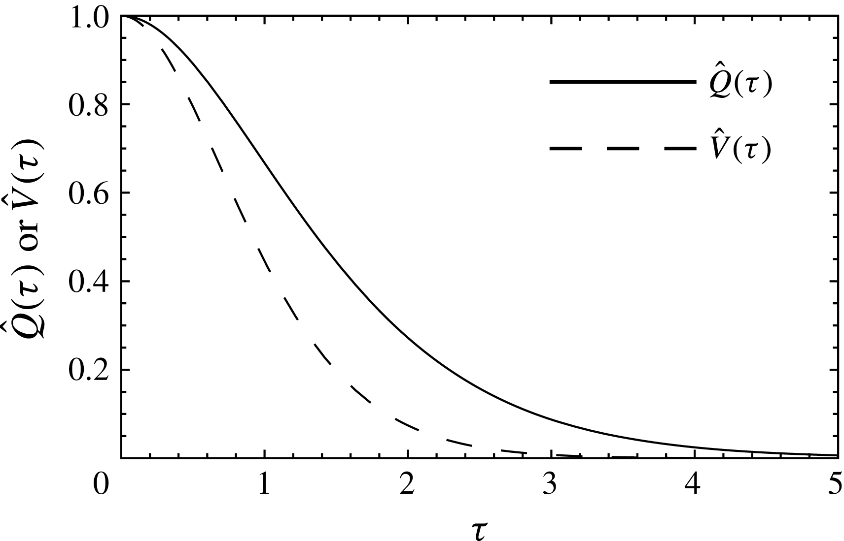
the numerical result of which is shown in figure 1, along with that of
 $\hat{V}(\unicode[STIX]{x1D70F})$
. This figure indicates that the integral time scale of
 $\hat{V}(\unicode[STIX]{x1D70F})$
is shorter than that of
 $\hat{Q}(\unicode[STIX]{x1D70F})$
, which is reasonable because
 $\hat{V}(\unicode[STIX]{x1D70F})$
includes the effect of the diffusion of two fluid particles.
Two velocity correlation functions
 $\hat{Q}(\unicode[STIX]{x1D70F})$
and
 $\hat{V}(\unicode[STIX]{x1D70F})$
plotted against
 $\unicode[STIX]{x1D70F}=C_{K}^{1/2}\unicode[STIX]{x1D700}^{1/3}k^{2/3}t$
.

Substituting (3.10) into (4.2) and applying (4.3) yields
 $$\begin{eqnarray}\displaystyle C_{K}^{-3/2} & = & \displaystyle \int _{0}^{1}\text{d}p\log \frac{1}{p}\int _{\max (p,1-p)}^{1+p}\text{d}q\,(pq)^{-8/3}\nonumber\\ \displaystyle & & \displaystyle \times \,\left\{b(1,p,q)\int _{0}^{\infty }\text{d}t\,[\hat{Q}(q^{2/3}t)]^{2}([\hat{Q}(p^{2/3}t)]^{2}-p^{11/3}[\hat{Q}(t)]^{2})+(p\leftrightarrow q)\right\}.\nonumber\\ \displaystyle & & \displaystyle\end{eqnarray}$$
The numerical computation of (4.10) and (4.11) yields
 $$\begin{eqnarray}C_{K}=1.779\end{eqnarray}$$
in the limit of an infinite Reynolds number. This value is close to both
 $1.62\pm 0.17$
, which is the mean of numerous experimental and observational data for different turbulent flows (Sreenivasan Reference Sreenivasan1995), and 1.58, which is the mean of direct numerical simulation data for
 $240\leqslant R_{\unicode[STIX]{x1D706}}\leqslant 1000$
(Donzis & Sreenivasan Reference Donzis and Sreenivasan2010), where
 $R_{\unicode[STIX]{x1D706}}$
is the Taylor-scale Reynolds number. The other previously developed closure models with no adjustable free parameters for high Reynolds numbers yield the following values for the Kolmogorov constant:
-
(i)
 $C_{K}=1.77$
(Kraichnan Reference Kraichnan1966) for the abridged Lagrangian DIA,
-
(ii)
$C_{K}=2.3$
(McComb & Shanmugasundaram Reference McComb and Shanmugasundaram1984) for the LET model, -
(iii)
$C_{K}=1.72$
(Kaneda Reference Kaneda1986; Kida & Goto Reference Kida and Goto1997) for the Lagrangian DIA, -
(iv)
$C_{K}=3.8$
(Edwards & McComb Reference Edwards and McComb1969) and
$C_{K}=1.2$
(Qian Reference Qian1983) for the Fokker–Planck model, -
(v)
$C_{K}=1.73$
(Bos & Bertoglio Reference Bos and Bertoglio2006) for the EDQNM.


4.2 Universal equilibrium range
Let us consider the energy spectrum throughout the universal equilibrium range, which constitutes the inertial and dissipation ranges. In this range, the mean energy dissipation rate
 $\unicode[STIX]{x1D700}$
per unit mass and the kinematic viscosity
 $\unicode[STIX]{x1D708}$
are the only parameters in the closure equations (3.4), (3.10) and (3.12); hence, dimensional analysis yields
 $$\begin{eqnarray}Q(k,t)=\frac{1}{2\unicode[STIX]{x03C0}}C_{K}\unicode[STIX]{x1D700}^{2/3}k^{-11/3}\tilde{Q}(\unicode[STIX]{x1D705},\unicode[STIX]{x1D70F}),\end{eqnarray}$$
where
 $$\begin{eqnarray}\unicode[STIX]{x1D705}=C_{K}^{-3/8}\unicode[STIX]{x1D700}^{-1/4}\unicode[STIX]{x1D708}^{3/4}k=C_{K}^{-3/8}k\unicode[STIX]{x1D702},\quad \unicode[STIX]{x1D70F}=C_{K}^{1/2}\unicode[STIX]{x1D700}^{1/3}k^{2/3}t\end{eqnarray}$$
and
 $$\begin{eqnarray}\tilde{Q}(0,\unicode[STIX]{x1D70F})=\hat{Q}(\unicode[STIX]{x1D70F}).\end{eqnarray}$$
Here,
 $\unicode[STIX]{x1D702}\;(=\unicode[STIX]{x1D700}^{-1/4}\unicode[STIX]{x1D708}^{3/4})$
denotes the Kolmogorov length scale, and
 $\hat{Q}(\unicode[STIX]{x1D70F})$
is defined in (4.3).
Substituting (4.13) into (3.4) and (3.12) respectively yields
 $$\begin{eqnarray}\left[\frac{\unicode[STIX]{x2202}}{\unicode[STIX]{x2202}\unicode[STIX]{x1D70F}}+\unicode[STIX]{x1D705}^{4/3}\right]\tilde{Q}(\unicode[STIX]{x1D705},\unicode[STIX]{x1D70F})=-\tilde{Q}(\unicode[STIX]{x1D705},\unicode[STIX]{x1D70F})\int _{0}^{\infty }\text{d}p\,J(p)\int _{0}^{\unicode[STIX]{x1D70F}}\text{d}t\,\tilde{Q}(\unicode[STIX]{x1D705}p^{3/2},pt)\end{eqnarray}$$
and
 $$\begin{eqnarray}\displaystyle \tilde{Q}(\unicode[STIX]{x1D705},0) & = & \displaystyle \frac{1}{2}\iint _{I_{\unicode[STIX]{x1D705}}}\text{d}p\,\text{d}q\,\unicode[STIX]{x1D705}^{-1}(pq)^{-8/3}b(\unicode[STIX]{x1D705},p,q)\int _{0}^{\infty }\text{d}t\exp [-(\unicode[STIX]{x1D705}^{2}+p^{2}+q^{2})t]\nonumber\\ \displaystyle & & \displaystyle \times \,\frac{[\tilde{Q}(q,q^{2/3}t)]^{2}}{\tilde{Q}(q,0)}\left\{\unicode[STIX]{x1D705}^{11/3}\frac{[\tilde{Q}(p,p^{2/3}t)]^{2}}{\tilde{Q}(p,0)}-p^{11/3}\frac{[\tilde{Q}(\unicode[STIX]{x1D705},\unicode[STIX]{x1D705}^{2/3}t)]^{2}}{\tilde{Q}(\unicode[STIX]{x1D705},0)}\right\},\end{eqnarray}$$
where (3.10) was used. The formal solution of (4.16) is given by
 $$\begin{eqnarray}\log \frac{\tilde{Q}(\unicode[STIX]{x1D705},\unicode[STIX]{x1D70F})}{\tilde{Q}(\unicode[STIX]{x1D705},0)}=-\unicode[STIX]{x1D705}^{4/3}\unicode[STIX]{x1D70F}-\int _{0}^{\infty }\text{d}p\,J(p)\int _{0}^{\unicode[STIX]{x1D70F}}\text{d}t\,(\unicode[STIX]{x1D70F}-t)\tilde{Q}(\unicode[STIX]{x1D705}p^{3/2},pt).\end{eqnarray}$$
Substituting (4.13) into (2.38) yields the compensated energy spectrum
 $$\begin{eqnarray}\tilde{Q}(\unicode[STIX]{x1D705},0)=\frac{k^{5/3}E(k)}{C_{K}\unicode[STIX]{x1D700}^{2/3}}.\end{eqnarray}$$
The numerical result
 $\tilde{Q}(\unicode[STIX]{x1D705},\unicode[STIX]{x1D70F})$
of (4.17) and (4.18) at
 $\unicode[STIX]{x1D70F}=0$
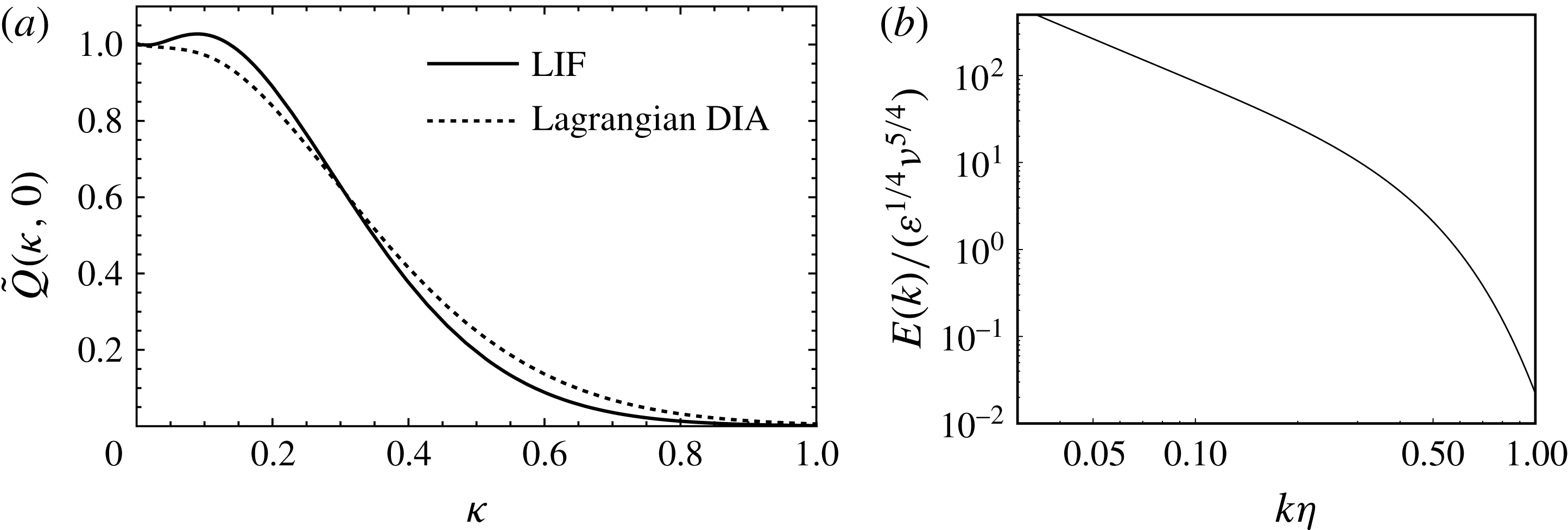
for the LIF model, along with that for the Lagrangian DIA (Kaneda Reference Kaneda1986; Kida & Goto Reference Kida and Goto1997) and the corresponding energy spectrum
 $E(k)$
for the LIF model are shown in figure 2. Figure 2(a) indicates that the LIF model reproduces the bottleneck effect (a small bump at
 $\unicode[STIX]{x1D705}\approx 0.1$
), whereas the Lagrangian DIA does not (see also figure 4). The compensated energy spectrum
 $\tilde{Q}(\unicode[STIX]{x1D705},0)$
attains a maximum value of 1.02 at
 $k\unicode[STIX]{x1D702}=C_{K}^{3/8}\unicode[STIX]{x1D705}=0.11$
, which is close to the value of 0.13 obtained from the direct numerical simulation by Donzis & Sreenivasan (Reference Donzis and Sreenivasan2010). They stated that the bottleneck decreases with increasing Reynolds number and would be negligible at
 $R_{\unicode[STIX]{x1D706}}\sim 2\times 10^{5}$
. This statement is not incompatible with the obtained peak value of
 $1.02\approx 1$
for the LIF model in the limit of an infinite Reynolds number.
(a) Compensated energy spectra
 $\tilde{Q}(\unicode[STIX]{x1D705},0)$
plotted against
 $\unicode[STIX]{x1D705}=C_{K}^{-3/8}k\unicode[STIX]{x1D702}$
for the LIF model and the Lagrangian DIA. (b) Log–log plot of the energy spectrum
 $E(k)/(\unicode[STIX]{x1D700}^{1/4}\unicode[STIX]{x1D708}^{5/4})$
plotted against
 $k\unicode[STIX]{x1D702}$
for the LIF model.

The skewness
 $S$
of the longitudinal velocity derivative in stationary homogeneous isotropic turbulence is expressed as (see (7.5.15) in Batchelor (Reference Batchelor1953))
 $$\begin{eqnarray}S=\frac{\displaystyle \left\langle \left({\displaystyle \frac{\unicode[STIX]{x2202}u_{1}}{\unicode[STIX]{x2202}x_{1}}}\right)^{3}\right\rangle }{\displaystyle \left\langle \left({\displaystyle \frac{\unicode[STIX]{x2202}u_{1}}{\unicode[STIX]{x2202}x_{1}}}\right)^{2}\right\rangle ^{3/2}}=-\frac{3\sqrt{30}\,\unicode[STIX]{x1D708}}{7}\frac{\displaystyle \int _{0}^{\infty }\text{d}k\,k^{4}E(k)}{\displaystyle \left[\int _{0}^{\infty }\text{d}k\,k^{2}E(k)\right]^{3/2}}=-\frac{3\sqrt{30}}{7}\frac{\displaystyle \int _{0}^{\infty }\text{d}\unicode[STIX]{x1D705}\unicode[STIX]{x1D705}^{7/3}\tilde{Q}(\unicode[STIX]{x1D705},0)}{\displaystyle \left[\displaystyle \int _{0}^{\infty }\text{d}\unicode[STIX]{x1D705}\unicode[STIX]{x1D705}^{1/3}\tilde{Q}(\unicode[STIX]{x1D705},0)\right]^{3/2}},\end{eqnarray}$$
where (4.14a
) and (4.19) were used. Substituting the numerical result
 $\tilde{Q}(\unicode[STIX]{x1D705},0)$
into (4.20) yields
 $$\begin{eqnarray}S=-0.49\end{eqnarray}$$
in the limit of an infinite Reynolds number. Antonia et al. (Reference Antonia, Tang, Djenidi and Danaila2015) reexamined numerous experimental and numerical data for different turbulent flows, with the result that the skewness
 $S$
should approach a constant value of
 $-0.53$
when the Reynolds number is sufficiently large (see also Sreenivasan & Antonia Reference Sreenivasan and Antonia1997). The other closure models for high Reynolds numbers yield the following values for the skewness:
-
(i)
$S=-0.35$
(McComb & Shanmugasundaram Reference McComb and Shanmugasundaram1984) for the LET model, -
(ii)
$S=-0.66$
(Kaneda Reference Kaneda1993; Kida & Goto Reference Kida and Goto1997) for the Lagrangian DIA, -
(iii)
$S=-0.515$
(Qian Reference Qian1994) for the Fokker–Planck model, -
(iv)
$S=-0.4$
(Bos et al.
Reference Bos, Chevillard, Scott and Rubinstein2012) for the EDQNM.


Substituting (4.13) into (4.1) yields
 $$\begin{eqnarray}\frac{1}{2}C_{K}^{-3/2}=\int _{0}^{\infty }\text{d}\unicode[STIX]{x1D705}\unicode[STIX]{x1D705}^{1/3}\tilde{Q}(\unicode[STIX]{x1D705},0),\end{eqnarray}$$
which is useful to check the numerical result
 $\tilde{Q}(\unicode[STIX]{x1D705},\unicode[STIX]{x1D70F})$
of (4.17) and (4.18). Substituting the numerical result
 $\tilde{Q}(\unicode[STIX]{x1D705},0)$
into (4.22) yields
 $C_{K}=1.78$
, which is very close to (4.12).
5 Discussion
5.1 Comparison of the LIF and QN models
The closure procedure in the LIF model is compared with that in the QN model. To this end, the QN procedure is first described in a similar manner to that of the LIF procedure in § 3.
The evolution equations of the second- and third-order moments are symbolically expressed as
 $$\begin{eqnarray}\left[\frac{\unicode[STIX]{x2202}}{\unicode[STIX]{x2202}t}+\unicode[STIX]{x1D708}\right]\langle uu\rangle =\langle uuu\rangle\end{eqnarray}$$
and
 $$\begin{eqnarray}\left[\frac{\unicode[STIX]{x2202}}{\unicode[STIX]{x2202}t}+\unicode[STIX]{x1D708}\right]\langle uuu\rangle =\langle uuuu\rangle ,\end{eqnarray}$$
respectively. The formal solution to (5.2) is
 $$\begin{eqnarray}\langle uuu\rangle =\int \text{d}t\,\text{e}^{-\unicode[STIX]{x1D708}t}\langle uuuu\rangle .\end{eqnarray}$$
Note that
 $\langle vvvv\rangle$
in (3.16) is the Lagrangian two-time correlation while
 $\langle uuuu\rangle$
in (5.3) is the Eulerian single-time correlation. Substituting (5.3) into (5.1) and assuming that
 $u$
has a Gaussian distribution yields the following closure equation for
 $\langle uu\rangle$
:
 $$\begin{eqnarray}\frac{\unicode[STIX]{x2202}}{\unicode[STIX]{x2202}t}\langle uu\rangle =-\unicode[STIX]{x1D708}\langle uu\rangle +\int \text{d}t\,\text{e}^{-\unicode[STIX]{x1D708}t}\langle uu\rangle \langle uu\rangle .\end{eqnarray}$$
Only the fourth-order moment is modelled with a Gaussian distribution; for example,
 $\langle uuu\rangle \neq 0$
.
The most significant difference between the QN and LIF models is that the QN model uses the solution (5.3) to the evolution equation (5.2) as the mean value, whereas the LIF model uses the solution (3.15) to the evolution equation (3.14) as a raw (non-mean) value. Hence, the latter properly considers a given realization of turbulence. In closure models, the most important procedure is the construction of the fourth-order moment
 $\langle uuuu\rangle$
from the third-order moment
 $\langle uuu\rangle$
. In this procedure, the QN model uses (5.3), which omits the information on individual raw motion by considering the average value, whereas the LIF model uses (3.15), which includes the information on individual raw motion; hence, the QN model fails to consider the eddy damping effect, whereas the LIF model successfully considers this effect.
Let us discuss the realizability that the probability distribution of realizations is non-negative. In turbulence theory, the realizability is important and must be satisfied. Using (2.30) and (2.35), the realizability condition is expressed by
 $$\begin{eqnarray}\breve{Q}(k,t,t)\geqslant 0.\end{eqnarray}$$
It is well known that the QN model fails to satisfy the realizability condition (Ogura Reference Ogura1963). Although the structure of the energy equation in the LIF model is similar to that in the QN model, the LIF model satisfies the realizability condition (5.5) mainly because the LIF model treats the two-time correlation while the QN model only involves the single-time correlation. A proof of the realizability is given in appendix G. Note that the QN model satisfies the realizability condition after a Markovian modification (Orszag Reference Orszag1977). Incidentally, the Eulerian DIA and the EDQNM are realizable, and the Lagrangian DIA (Kaneda Reference Kaneda1986; Kida & Goto Reference Kida and Goto1997) can only be checked numerically to be realizable.
5.2 Two assumptions
Assumptions (i ′ ) and (ii) are discussed here.
First, consider assumptions (i
′
) omitting ‘approximately’ and (ii). Substituting
 $u=v\unicode[STIX]{x1D713}$
into
 $\langle uuu\rangle$
and applying these two assumptions yields, instead of (3.16),
 $$\begin{eqnarray}\langle uuu\rangle =\langle v\unicode[STIX]{x1D713}v\unicode[STIX]{x1D713}v\unicode[STIX]{x1D713}\rangle =\langle vvv\rangle =0,\end{eqnarray}$$
which is an undesirable result. Another example similar to that described above is also given here. Substituting
 $u=v\unicode[STIX]{x1D713}$
into
 $\langle uu\rangle$
and applying assumption (i
′
) omitting ‘approximately’ yields
 $$\begin{eqnarray}\langle uu\rangle =\langle v\unicode[STIX]{x1D713}v\unicode[STIX]{x1D713}\rangle =\langle vv\rangle ,\end{eqnarray}$$
which shows that the Lagrangian velocity correlation function is consistent with the Eulerian one. However, this is not completely acceptable, because a direct numerical simulation shows that the characteristic time scale of the Lagrangian velocity correlation function varies as
 $k^{-2/3}$
in the inertial range, whereas that of the Eulerian function varies as
 $k^{-1}$
(Kaneda, Ishihara & Gotoh Reference Kaneda, Ishihara and Gotoh1999).
Second, to overcome these difficulties, consider assumption (i
′
) with ‘approximately’ systematically by introducing a small parameter
 $\unicode[STIX]{x1D716}$
as follows:
 $$\begin{eqnarray}\langle vv\rangle =O(1),\quad \langle vvv\rangle =0,\quad \langle vvvv\rangle =\langle vv\rangle \langle vv\rangle =O(1),\quad \langle vvvvv\rangle =0,\end{eqnarray}$$
 $$\begin{eqnarray}\langle v^{n}\unicode[STIX]{x1D713}^{m}\rangle =\langle v^{n}\rangle \langle \unicode[STIX]{x1D713}^{m}\rangle +O(\unicode[STIX]{x1D716}),\quad \langle \unicode[STIX]{x1D713}\rangle =O(1),\end{eqnarray}$$
where
 $\unicode[STIX]{x1D716}$
is defined as
 $$\begin{eqnarray}\unicode[STIX]{x1D716}g(\boldsymbol{k},\boldsymbol{k}^{\prime },t,t^{\prime })=\langle v_{i}(t|\boldsymbol{k},t^{\prime })v_{i}(t|\boldsymbol{k}^{\prime },t^{\prime })\unicode[STIX]{x1D713}(\boldsymbol{k},t|\boldsymbol{k}^{\prime },t^{\prime })\rangle -\langle v_{i}(t|\boldsymbol{k},t^{\prime })v_{i}(t|\boldsymbol{k}^{\prime },t^{\prime })\rangle \langle \unicode[STIX]{x1D713}(\boldsymbol{k},t|\boldsymbol{k}^{\prime },t^{\prime })\rangle .\end{eqnarray}$$
Here
 $g(\boldsymbol{k},\boldsymbol{k}^{\prime },t,t^{\prime })$
is an appropriate function with the dimension of
 $v^{2}\unicode[STIX]{x1D713}$
and is
 $O(1)$
. Note that
 $\unicode[STIX]{x1D716}$
indicates the strength of statistical independence of
 $v$
and
 $\unicode[STIX]{x1D713}$
;
 $\unicode[STIX]{x1D716}=0$
denotes the complete independence. In the present approximation,
 $O(\unicode[STIX]{x1D716}^{2})$
is omitted. Using (5.9a
), equation (A 3) becomes
 $$\begin{eqnarray}\langle \unicode[STIX]{x1D713}^{m}\rangle =\langle \unicode[STIX]{x1D713}\rangle ^{m}+O(\unicode[STIX]{x1D716}).\end{eqnarray}$$
The first example
 $\langle uuu\rangle$
is reconsidered. Substituting
 $u=v\unicode[STIX]{x1D713}$
into
 $\langle uuu\rangle$
and applying (5.8), (5.9) and (5.11) yields
 $$\begin{eqnarray}\langle uuu\rangle =\langle v\unicode[STIX]{x1D713}v\unicode[STIX]{x1D713}v\unicode[STIX]{x1D713}\rangle =\langle vvv\rangle \langle \unicode[STIX]{x1D713}\unicode[STIX]{x1D713}\unicode[STIX]{x1D713}\rangle +O(\unicode[STIX]{x1D716})=O(\unicode[STIX]{x1D716})\neq 0\end{eqnarray}$$
instead of
 $\langle uuu\rangle =0$
in (5.6). In the second example, substituting
 $u=v\unicode[STIX]{x1D713}$
into
 $\langle uu\rangle$
and applying (5.8), (5.9) and (5.11) yields
 $$\begin{eqnarray}\langle uu\rangle =\langle v\unicode[STIX]{x1D713}v\unicode[STIX]{x1D713}\rangle =\langle vv\rangle \langle \unicode[STIX]{x1D713}\unicode[STIX]{x1D713}\rangle +O(\unicode[STIX]{x1D716})=\langle vv\rangle +O(\unicode[STIX]{x1D716})\neq \langle vv\rangle\end{eqnarray}$$
instead of
 $\langle uu\rangle =\langle vv\rangle$
in (5.7).
Another expression of the third-order moment
 $\langle uuu\rangle$
is also considered. Averaging (3.15) and applying (2.21), (5.8), (5.9) and (5.11) yields
 $$\begin{eqnarray}\langle uuu\rangle =\int \text{d}t\,\text{e}^{-\unicode[STIX]{x1D708}t}\langle v\unicode[STIX]{x1D713}v\unicode[STIX]{x1D713}v\unicode[STIX]{x1D713}v\unicode[STIX]{x1D713}\rangle =\int \text{d}t\,\text{e}^{-\unicode[STIX]{x1D708}t}[\langle vvvv\rangle \langle \unicode[STIX]{x1D713}\unicode[STIX]{x1D713}\unicode[STIX]{x1D713}\unicode[STIX]{x1D713}\rangle +O(\unicode[STIX]{x1D716})]=\int \text{d}t\,\text{e}^{-\unicode[STIX]{x1D708}t}\langle vvvv\rangle ,\end{eqnarray}$$
which is consistent with (5.12) when
 $$\begin{eqnarray}\int \text{d}t\,\text{e}^{-\unicode[STIX]{x1D708}t}\langle vvvv\rangle =O(\unicode[STIX]{x1D716}).\end{eqnarray}$$
In practice, equation (3.16) (or (5.14)) should be used instead of (5.12) for the closure procedure of
 $\langle uuu\rangle$
because (5.12) gives no useful information.
Hence, it is reasonable to suppose that assumption (i ′ ) is approximately applied while assumption (ii) is strictly applied.
5.3 Comparison of the LIF model and the Lagrangian DIA in the inertial range
First, the energy balance equation in the LIF model is compared with that in the Lagrangian DIA (Kaneda Reference Kaneda1981; Kida & Goto Reference Kida and Goto1997) in the inertial range. The latter is expressed as
 $$\begin{eqnarray}\displaystyle C_{K}^{-3/2} & = & \displaystyle \int _{0}^{1}\text{d}p\log \frac{1}{p}\int _{\max (p,1-p)}^{1+p}\text{d}q\,(pq)^{-8/3}\nonumber\\ \displaystyle & & \displaystyle \times \,\left[b(1,p,q)\int _{0}^{\infty }\text{d}t\,\hat{Q}(t)\hat{Q}(p^{2/3}t)\hat{Q}(q^{2/3}t)(1-p^{11/3})+(p\leftrightarrow q)\right]\end{eqnarray}$$
in the present notation. The main difference between (4.11) and (5.16) is their time dependence, including the number of times the correlation function
 $\hat{Q}(t)$
appears in each model (four in the former and three in the latter).
Second, the localness of energy transfers in the LIF model is compared with that in the Lagrangian DIA in the inertial range. Both (4.11) and (5.16) can be rewritten in the form (Kraichnan Reference Kraichnan1966; Kaneda Reference Kaneda1986)
 $$\begin{eqnarray}\unicode[STIX]{x1D700}=\int _{1}^{\infty }W(\unicode[STIX]{x1D6FC})\frac{\text{d}\unicode[STIX]{x1D6FC}}{\unicode[STIX]{x1D6FC}},\end{eqnarray}$$
where
 $$\begin{eqnarray}W(\unicode[STIX]{x1D6FC})=\frac{\log \unicode[STIX]{x1D6FC}}{\unicode[STIX]{x1D6FC}}\int _{1}^{\unicode[STIX]{x1D6FC}^{\dagger }}\text{d}\unicode[STIX]{x1D6FD}\,T\left(1,\frac{1}{\unicode[STIX]{x1D6FC}},\frac{1}{\unicode[STIX]{x1D6FD}}\right)\frac{1}{\unicode[STIX]{x1D6FD}^{2}}+\unicode[STIX]{x1D6FC}\int _{\unicode[STIX]{x1D6FC}^{\ddagger }}^{\unicode[STIX]{x1D6FC}}\text{d}\unicode[STIX]{x1D6FD}\,T\left(1,\frac{1}{\unicode[STIX]{x1D6FD}},\frac{\unicode[STIX]{x1D6FC}}{\unicode[STIX]{x1D6FD}}\right)\frac{\log \unicode[STIX]{x1D6FD}}{\unicode[STIX]{x1D6FD}^{3}}.\end{eqnarray}$$
In (5.18),
 $\unicode[STIX]{x1D6FC}^{\dagger }=\min [\unicode[STIX]{x1D6FC},\unicode[STIX]{x1D6FC}/(\unicode[STIX]{x1D6FC}-1)]$
,
 $\unicode[STIX]{x1D6FC}^{\ddagger }=\max [1,\unicode[STIX]{x1D6FC}-1]$
and
 $$\begin{eqnarray}T(k,p,q)=16\unicode[STIX]{x03C0}^{2}kpq\,\hat{T}(k,p,q),\end{eqnarray}$$
where
 $$\begin{eqnarray}\hat{T}(\boldsymbol{k},\boldsymbol{p},\boldsymbol{q})\unicode[STIX]{x1D6FF}(\boldsymbol{k}-\boldsymbol{p}-\boldsymbol{q})=\unicode[STIX]{x1D614}_{nab}(\boldsymbol{k})\langle u_{a}(\,\boldsymbol{p},t)u_{b}(\boldsymbol{q},t)u_{n}(-\boldsymbol{k},t)\rangle .\end{eqnarray}$$
Because
 $\unicode[STIX]{x1D6FC}$
is the ratio of the maximum wavenumber involved in the triad interaction to the minimum wavenumber,
 $W(\unicode[STIX]{x1D6FC})\,\text{d}\unicode[STIX]{x1D6FC}/\unicode[STIX]{x1D6FC}$
is the contribution of the wavenumber ratios in the range
 $(\unicode[STIX]{x1D6FC},\unicode[STIX]{x1D6FC}+\text{d}\unicode[STIX]{x1D6FC})$
to the transport power. Kolmogorov’s hypothesis regarding the localness of energy transfers means that
 $W(\unicode[STIX]{x1D6FC})$
should decrease rapidly for
 $\unicode[STIX]{x1D6FC}\gg 1$
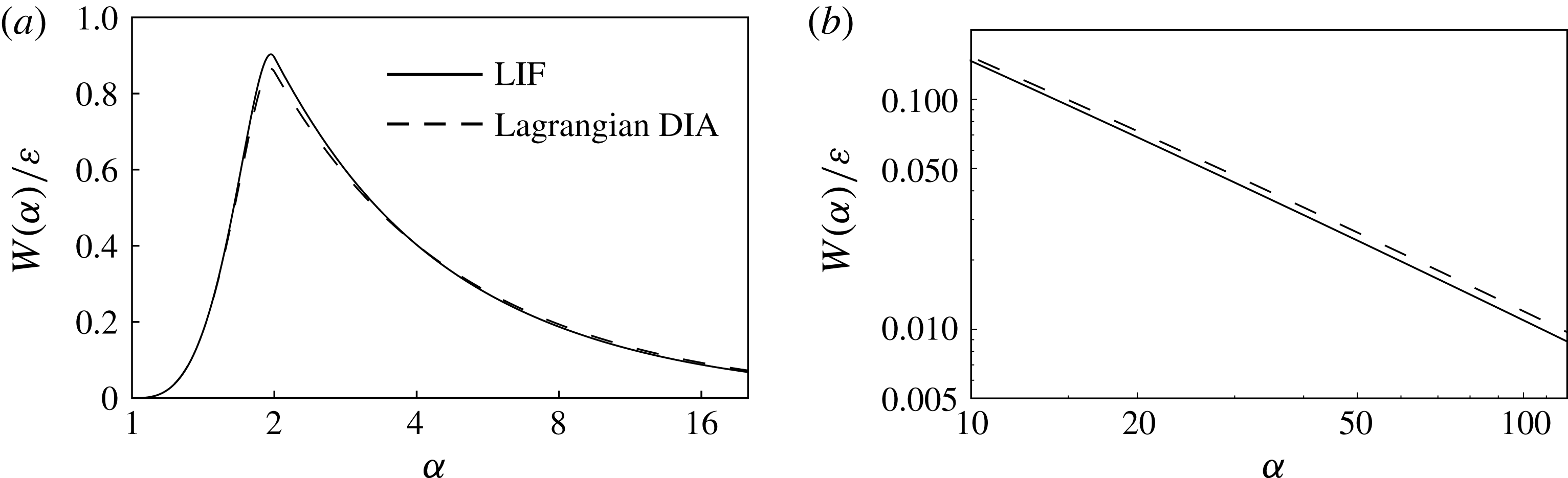
. Figure 3 shows the dependence of
 $W(\unicode[STIX]{x1D6FC})/\unicode[STIX]{x1D700}$
on the wavenumber ratio
 $\unicode[STIX]{x1D6FC}$
in the LIF model (solid line) and the Lagrangian DIA (dashed line). This figure indicates that
 $W(\unicode[STIX]{x1D6FC})$
in the LIF model is effectively identical to that in the Lagrangian DIA;
 $W(\unicode[STIX]{x1D6FC})$
has a peak at
 $\unicode[STIX]{x1D6FC}\approx 2$
and decreases gradually as
 $W(\unicode[STIX]{x1D6FC})=C/\unicode[STIX]{x1D6FC}$
for
 $\unicode[STIX]{x1D6FC}\gg 1$
, which differs slightly from
 $W(\unicode[STIX]{x1D6FC})\propto \unicode[STIX]{x1D6FC}^{-4/3}\log \unicode[STIX]{x1D6FC}$
(Kraichnan Reference Kraichnan1966). The value of
 $C$
in the LIF model is somewhat smaller than that in the Lagrangian DIA. This means that
 $C$
is related to the time dependence in (4.11) and (5.16) but the power of
 $\unicode[STIX]{x1D6FC}$
in
 $W(\unicode[STIX]{x1D6FC})$
is not.
(a) Linear–log and (b) log–log plots of
 $W(\unicode[STIX]{x1D6FC})/\unicode[STIX]{x1D700}$
for the LIF model and the Lagrangian DIA.

Figure 3 also indicates that Kolmogorov’s hypothesis regarding the localness of energy transfers is not completely satisfied in either of these models, because
 $W(\unicode[STIX]{x1D6FC})$
has a peak at
 $\unicode[STIX]{x1D6FC}\approx 2$
and decreases gradually, the locality of which is here called the weak non-locality of the triad interaction.
5.4 Bottleneck effect
This subsection presents a physical explanation of the bottleneck effect (Herring et al.
Reference Herring, Schertzer, Lesieur, Newman, Chollet and Larcheveque1982; Falkovich Reference Falkovich1994; Lohse & Müllergroeling Reference Lohse and Müllergroeling1995) on the basis of the LIF model. The energy flux
 $\unicode[STIX]{x1D6F1}(k)$
is expressed as (Kraichnan Reference Kraichnan1966)
 $$\begin{eqnarray}\unicode[STIX]{x1D6F1}(k)=\int _{k}^{\infty }\text{d}k^{\prime }\int _{0}^{k}\text{d}p^{\prime }\int _{\max (p^{\prime },k^{\prime }-p^{\prime })}^{p^{\prime }+k^{\prime }}\text{d}q^{\prime }\,T(k^{\prime },p^{\prime },q^{\prime })\quad (\boldsymbol{k}^{\prime }=\boldsymbol{p}^{\prime }+\boldsymbol{q}^{\prime }),\end{eqnarray}$$
which represents the net energy transfer from wavenumbers below
 $k$
to wavenumbers above
 $k$
. Considering the triad interaction as
 $p^{\prime }<k<k^{\prime }\sim q^{\prime }$
, the energy transfer
 $T(k^{\prime },p^{\prime },q^{\prime })$
in (E 13) is reduced very little for
 $p^{\prime }<k^{\prime }\sim q^{\prime }<1/\unicode[STIX]{x1D702}$
because the wavenumbers
 $k^{\prime }$
,
 $p^{\prime }$
,
 $q^{\prime }$
lie within the inertial range and hence
 $\text{e}^{-\unicode[STIX]{x1D708}[(k^{\prime })^{2}+(p^{\prime })^{2}+(q^{\prime })^{2}]t}\approx 1$
, whereas
 $T(k^{\prime },p^{\prime },q^{\prime })$
is substantially reduced for
 $p^{\prime }<1/\unicode[STIX]{x1D702}<k^{\prime }\sim q^{\prime }$
because
 $\text{e}^{-\unicode[STIX]{x1D708}[(k^{\prime })^{2}+(p^{\prime })^{2}+(q^{\prime })^{2}]t}<1$
. As a result of the local interaction,
 $k^{\prime }$
is nearly equal to
 $k$
because
 $p^{\prime }\lesssim k\lesssim k^{\prime }\sim q^{\prime }$
. Hence, the constancy of
 $\unicode[STIX]{x1D6F1}(k)$
in the inertial range implies that
 $u_{i}(\boldsymbol{k})$
should increase. The larger the wavenumber
 $k$
, the stronger the reduction effect of
 $T(k^{\prime },p^{\prime },q^{\prime })$
. This means that a substantial increase in
 $u_{i}(\boldsymbol{k})$
appears in the near-dissipation range (the right end of the inertial range). In the dissipation range (
 $k\gg 1/\unicode[STIX]{x1D702}$
), the term except
 $\text{e}^{-\unicode[STIX]{x1D708}[k^{2}+p^{2}+q^{2}]t}$
in (E 13) is also very small, and hence the reduction effect due to
 $\text{e}^{-\unicode[STIX]{x1D708}[(k^{\prime })^{2}+(p^{\prime })^{2}+(q^{\prime })^{2}]t}$
is unimportant and a bump is not observed. Therefore, the bottleneck effect is observed especially strongly in the near-dissipation range because of the weak non-locality of the triad interaction.
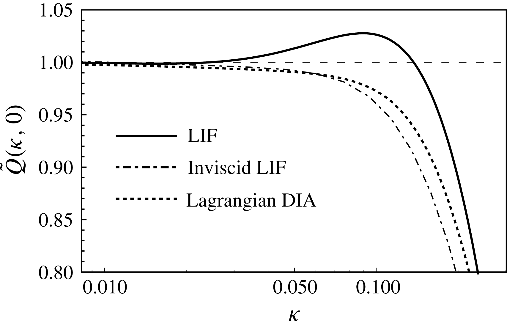
Linear–log plot of the compensated energy spectra
 $\tilde{Q}(\unicode[STIX]{x1D705},0)$
for the LIF model, the inviscid LIF model and the Lagrangian DIA plotted against
 $\unicode[STIX]{x1D705}=C_{K}^{-3/8}k\unicode[STIX]{x1D702}$
. The dashed line shows
 $\tilde{Q}(\unicode[STIX]{x1D705},0)=1$
.

Figure 4 shows the compensated energy spectra
 $\tilde{Q}(\unicode[STIX]{x1D705},0)$
for the LIF model; the inviscid LIF model, which is the LIF model under the condition
 $\text{e}^{-(k^{2}+p^{2}+q^{2})t}=1$
in (4.17); and the Lagrangian DIA. This figure indicates that the bottleneck effect does not occur in the inviscid LIF model as clearly as in the Lagrangian DIA. The factor
 $\text{e}^{-(k^{2}+p^{2}+q^{2})t}$
is related to the viscous term, and hence the viscosity plays an important role in the bottleneck effect. Note that the compensated energy spectrum in the inviscid LIF model is similar to that in the Lagrangian DIA because these two models exhibit similar structures.
5.5 Importance of a mapping function
This subsection discusses why some closure models, such as the Lagrangian DIA (Kraichnan Reference Kraichnan1965; Kaneda Reference Kaneda1981; Kida & Goto Reference Kida and Goto1997) and the LET model (McComb Reference McComb1978), are compatible with the Kolmogorov
 $-5/3$
power law.
The Eulerian DIA (Kraichnan Reference Kraichnan1959) is incompatible with the Kolmogorov
 $-5/3$
power law because the response integral diverges at the lower limit of the wavenumber as the Reynolds number approaches infinity. Kraichnan (Reference Kraichnan1965) introduced the generalized velocity
 $v_{i}(t|\boldsymbol{k}^{\prime },t^{\prime })$
to remove this divergence and reproduce the Kolmogorov
 $-5/3$
power law. Kraichnan (Reference Kraichnan1964) stated that any Eulerian multi-time closure suffers from the difficulty associated with the violation of the invariance under the Galilean transformation and for this reason the Eulerian multi-time formation is intrinsically unsuitable for the derivation of the Kolmogorov
 $-5/3$
power law. However, this statement seems to be inconsistent with the case of the LET model (McComb Reference McComb1978), which is an Eulerian multi-time closure in the Eulerian framework that is compatible with the Kolmogorov
 $-5/3$
power law.
The focus of this discussion now shifts from the Galilean invariance to the use of a mapping function. The difference between the Eulerian DIA and the LET model is that the Eulerian DIA uses the response function
 $\unicode[STIX]{x1D60E}_{ij}(\boldsymbol{k},t|\boldsymbol{k}^{\prime },t^{\prime })$
, which is defined as
 $$\begin{eqnarray}\unicode[STIX]{x1D60E}_{ij}(\boldsymbol{k},t|\boldsymbol{k}^{\prime },t^{\prime })=\frac{\unicode[STIX]{x1D6FF}u_{i}(\boldsymbol{k},t)}{\unicode[STIX]{x1D6FF}u_{j}(\boldsymbol{k}^{\prime },t^{\prime })},\end{eqnarray}$$
whereas the LET model uses a mapping function
 $\unicode[STIX]{x1D60F}_{ij}(\boldsymbol{k}^{\prime },t^{\prime }|\boldsymbol{k},t)$
, which is defined as
 $$\begin{eqnarray}u_{i}(\boldsymbol{k},t)=(2\unicode[STIX]{x03C0})^{3}\int \text{d}\boldsymbol{k}^{\prime }\unicode[STIX]{x1D60F}_{ij}(\boldsymbol{k}^{\prime },t^{\prime }|\boldsymbol{k},t)u_{j}(\boldsymbol{k}^{\prime },t^{\prime }).\end{eqnarray}$$
The evolution equations of
 $\langle \unicode[STIX]{x1D60E}_{ij}(\boldsymbol{k},t|\boldsymbol{k}^{\prime },t^{\prime })\rangle$
and
 $\langle \unicode[STIX]{x1D60F}_{ij}(\boldsymbol{k}^{\prime },t^{\prime }|\boldsymbol{k},t)\rangle$
are symbolically expressed as
 $$\begin{eqnarray}\left[\frac{\unicode[STIX]{x2202}}{\unicode[STIX]{x2202}t}+\unicode[STIX]{x1D708}\right]\langle G\rangle =\unicode[STIX]{x1D706}\langle uG\rangle\end{eqnarray}$$
and
 $$\begin{eqnarray}\left[\frac{\unicode[STIX]{x2202}}{\unicode[STIX]{x2202}t}+\unicode[STIX]{x1D708}\right]\langle Huu\rangle =\unicode[STIX]{x1D706}\langle uuu\rangle ,\end{eqnarray}$$
respectively, where
 $\unicode[STIX]{x1D706}$
is a bookkeeping parameter. In the Eulerian DIA, substituting the perturbation expansions
 $u=u^{(0)}+\unicode[STIX]{x1D706}u^{(1)}+\cdots \,$
and
 $G=G^{(0)}+\unicode[STIX]{x1D706}G^{(1)}+\cdots \,$
into the right-hand side of (5.24), the renormalization procedure is applied for
 $u$
and
 $G$
, whereas in the LET model, substituting the perturbation expansion
 $u=u^{(0)}+\unicode[STIX]{x1D706}u^{(1)}+\cdots \,$
into the right-hand side of (5.25), the renormalization procedure is applied only for
 $u$
. The right-hand side of (5.25) is similar to that of (5.1), and the evolution equation of the correlation function
 $\langle uu\rangle$
is irrelevant to the divergence of the response integral at the lower limit of the wavenumber. As a result, the difference between the mapping function
 $H$
and the response function
 $G$
eliminates the divergence in the LET model, thus making the LET model compatible with the Kolmogorov
 $-5/3$
power law. For further details on the LET model, see § 7.4 in McComb (Reference McComb1990) and McComb & Yoffe (Reference McComb and Yoffe2017). The latter reference introduces a formal derivation of the LET model by using a fluctuation-dissipation relation.
In the Lagrangian DIA, Kraichnan (Reference Kraichnan1965) used the Lagrangian velocity response function
 $\unicode[STIX]{x1D60E}_{in}(\boldsymbol{k},t|s;\boldsymbol{k}^{\prime },t^{\prime }|s^{\prime })$
, which is defined as
 $$\begin{eqnarray}\unicode[STIX]{x1D60E}_{in}(\boldsymbol{k},t|s;\boldsymbol{k}^{\prime },t^{\prime }|s^{\prime })=\frac{\unicode[STIX]{x1D6FF}v_{i}(s|\boldsymbol{k},t)}{\unicode[STIX]{x1D6FF}v_{n}(s^{\prime }|\boldsymbol{k}^{\prime },t^{\prime })},\end{eqnarray}$$
with
 $$\begin{eqnarray}\unicode[STIX]{x1D60E}_{in}(\boldsymbol{k},t|t;\boldsymbol{k}^{\prime },t|t)=\unicode[STIX]{x1D6FF}_{in}\unicode[STIX]{x1D6FF}(\boldsymbol{k}+\boldsymbol{k}^{\prime }).\end{eqnarray}$$
The evolution equation of
 $\unicode[STIX]{x1D60E}_{nn}(\boldsymbol{k},t|t;\boldsymbol{k}^{\prime },t|s)$
is given by
 $$\begin{eqnarray}\frac{\unicode[STIX]{x2202}}{\unicode[STIX]{x2202}t}\unicode[STIX]{x1D60E}_{nn}(\boldsymbol{k},t|t;\boldsymbol{k}^{\prime },t|s)=-\text{i}k_{j}\iint \text{d}\boldsymbol{p}\,\text{d}\boldsymbol{q}\,\unicode[STIX]{x1D6FF}(\boldsymbol{k}-\boldsymbol{p}-\boldsymbol{q})u_{j}(\,\boldsymbol{p},t)\unicode[STIX]{x1D60E}_{nn}(\boldsymbol{q},t|t;\boldsymbol{k}^{\prime },t|s),\end{eqnarray}$$
with
 $\unicode[STIX]{x1D60E}_{nn}(\boldsymbol{k},t|t;\boldsymbol{k}^{\prime },t|t)=3\unicode[STIX]{x1D6FF}(\boldsymbol{k}+\boldsymbol{k}^{\prime })$
. The derivation of (5.28) is given in appendix H. Equation (5.28) is the same as the evolution equation of the Lagrangian position function in (2.26), and hence the Lagrangian velocity response function
 $\unicode[STIX]{x1D60E}_{in}(\boldsymbol{k},t|s;\boldsymbol{k}^{\prime },t^{\prime }|s^{\prime })$
also acts as a mapping function with respect to the labelling time of the generalized velocity, as shown in (2.3). Furthermore, Kaneda (Reference Kaneda1981) and Kida & Goto (Reference Kida and Goto1997) used (2.26). Hence, the Lagrangian DIA (Kraichnan Reference Kraichnan1965; Kaneda Reference Kaneda1981; Kida & Goto Reference Kida and Goto1997) uses a mapping function.
In summary, considering that both the LET model and the Lagrangian DIA use a mapping function but the Eulerian DIA does not, it is plausible to postulate that a key point in the derivation of the Kolmogorov
 $-5/3$
power law is the use of a mapping function in the closure procedure.
This paper presented the advantages of the LIF model over the Lagrangian DIA (Kraichnan Reference Kraichnan1965; Kaneda Reference Kaneda1981; Kida & Goto Reference Kida and Goto1997). The derivation of the closure equations in the LIF model is similar to that in the QN model and simpler than that in the Lagrangian DIA because the LIF model includes neither the response function nor the renormalized expansion.
Acknowledgements
The author thanks Y. Kaneda for his valuable discussion on the Eulerian DIA and the LET model, T. Gotoh for his useful comments on the Lagrangian velocity correlation function, S. Goto for his interesting comments on assumption (i ′ ) and Ooshida T. for his useful comments on the Lagrangian position function.
Appendix A
Substituting
 $\boldsymbol{k}=\boldsymbol{k}_{1}$
,
 $\boldsymbol{k}^{\prime }=\boldsymbol{k}_{1}^{\prime }$
,
 $t=t_{1}$
and
 $t^{\prime }=t_{1}^{\prime }$
into (2.26), multiplying the result by
 $\prod _{n=2}^{N}\unicode[STIX]{x1D713}(\boldsymbol{k}_{n},t_{n}|\boldsymbol{k}_{n}^{\prime },t_{n}^{\prime })$
, taking the average of the result and considering (2.24) and assumption (i
′
) yields
 $$\begin{eqnarray}\displaystyle & & \displaystyle \frac{\unicode[STIX]{x2202}}{\unicode[STIX]{x2202}t_{1}}\left\langle \mathop{\prod }_{n=1}^{N}\unicode[STIX]{x1D713}(\boldsymbol{k}_{n},t_{n}|\boldsymbol{k}_{n}^{\prime },t_{n}^{\prime })\right\rangle =-(2\unicode[STIX]{x03C0})^{3}\text{i}{k_{1}}_{j}\iiint \text{d}\boldsymbol{p}\,\text{d}\boldsymbol{q}\,\text{d}\boldsymbol{k}^{\prime \prime }\unicode[STIX]{x1D6FF}(\boldsymbol{k}_{1}-\boldsymbol{p}-\boldsymbol{q})\langle v_{j}(t_{1}|\boldsymbol{k}^{\prime \prime },T)\rangle \nonumber\\ \displaystyle & & \displaystyle \quad \times \,\left\langle \unicode[STIX]{x1D713}(-\boldsymbol{k}^{\prime \prime },T|\boldsymbol{p},t_{1})\unicode[STIX]{x1D713}(\boldsymbol{q},t_{1}|\boldsymbol{k}_{1}^{\prime },t_{1}^{\prime })\mathop{\prod }_{n=2}^{N}\unicode[STIX]{x1D713}(\boldsymbol{k}_{n},t_{n}|\boldsymbol{k}_{n}^{\prime },t_{n}^{\prime })\right\rangle =0,\end{eqnarray}$$
where (2.40) was applied. Equation (A 1) shows that
 $\langle \prod _{n=1}^{N}\unicode[STIX]{x1D713}(\boldsymbol{k}_{n},t_{n}|\boldsymbol{k}_{n}^{\prime },t_{n}^{\prime })\rangle$
is independent of
 $t_{1}$
. Using this independence, (2.25) and (3.2) yields
 $$\begin{eqnarray}\displaystyle \left\langle \mathop{\prod }_{n=1}^{N}\unicode[STIX]{x1D713}(\boldsymbol{k}_{n},t_{n}|\boldsymbol{k}_{n}^{\prime },t_{n}^{\prime })\right\rangle & = & \displaystyle \left\langle \unicode[STIX]{x1D713}(\boldsymbol{k}_{1},t_{1}^{\prime }|\boldsymbol{k}_{1}^{\prime },t_{1}^{\prime })\mathop{\prod }_{n=2}^{N}\unicode[STIX]{x1D713}(\boldsymbol{k}_{n},t_{n}|\boldsymbol{k}_{n}^{\prime },t_{n}^{\prime })\right\rangle \nonumber\\ \displaystyle & = & \displaystyle \langle \unicode[STIX]{x1D713}(\boldsymbol{k}_{1},t_{1}|\boldsymbol{k}_{1}^{\prime },t_{1}^{\prime })\rangle \left\langle \mathop{\prod }_{n=2}^{N}\unicode[STIX]{x1D713}(\boldsymbol{k}_{n},t_{n}|\boldsymbol{k}_{n}^{\prime },t_{n}^{\prime })\right\rangle .\end{eqnarray}$$
Repeating this procedure ultimately yields
 $$\begin{eqnarray}\left\langle \mathop{\prod }_{n=1}^{N}\unicode[STIX]{x1D713}(\boldsymbol{k}_{n},t_{n}|\boldsymbol{k}_{n}^{\prime },t_{n}^{\prime })\right\rangle =\mathop{\prod }_{n=1}^{N}\left\langle \unicode[STIX]{x1D713}(\boldsymbol{k}_{n},t_{n}|\boldsymbol{k}_{n}^{\prime },t_{n}^{\prime })\right\rangle .\end{eqnarray}$$
Thus, the Lagrangian position functions have been demonstrated to be statistically independent of each other.
Appendix B
Substituting (2.28) into (3.3) yields
 $$\begin{eqnarray}\displaystyle & & \displaystyle \frac{\unicode[STIX]{x2202}}{\unicode[STIX]{x2202}t}\unicode[STIX]{x1D618}_{bc}(\boldsymbol{k},t,t^{\prime })=\left[-(2\unicode[STIX]{x03C0})^{3}\unicode[STIX]{x1D708}\iint \text{d}\boldsymbol{k}^{\prime }\,\text{d}\boldsymbol{p}\,p^{2}\langle u_{a}(\,\boldsymbol{p},t)\unicode[STIX]{x1D713}(-\boldsymbol{p},t|\boldsymbol{k},t^{\prime })u_{b}(\boldsymbol{k}^{\prime },t^{\prime })\rangle \right.\nonumber\\ \displaystyle & & \displaystyle \quad +\,(2\unicode[STIX]{x03C0})^{3}\text{i}\iiiint \text{d}\boldsymbol{k}^{\prime }\,\text{d}\boldsymbol{p}\,\text{d}\boldsymbol{q}\,\text{d}\boldsymbol{r}\,\unicode[STIX]{x1D6FF}(\boldsymbol{r}-\boldsymbol{p}-\boldsymbol{q})\nonumber\\ \displaystyle & & \displaystyle \quad \times \,\frac{r_{a}r_{j}r_{m}}{r^{2}}\langle u_{j}(\,\boldsymbol{p},t)u_{m}(\boldsymbol{q},t)\unicode[STIX]{x1D713}(-\boldsymbol{r},t|\boldsymbol{k},t^{\prime })u_{b}(\boldsymbol{k}^{\prime },t^{\prime })\rangle \nonumber\\ \displaystyle & & \displaystyle \quad +\left.(2\unicode[STIX]{x03C0})^{3}\iint \text{d}\boldsymbol{k}^{\prime }\,\text{d}\boldsymbol{p}\langle f_{a}(\,\boldsymbol{p},t)\unicode[STIX]{x1D713}(-\boldsymbol{p},t|\boldsymbol{k},t^{\prime })u_{b}(\boldsymbol{k}^{\prime },t^{\prime })\rangle \right]\unicode[STIX]{x1D60B}_{ca}(\boldsymbol{k})\quad (t>t^{\prime }).\end{eqnarray}$$
First, the viscous term on the right-hand side of (B 1) is considered. Using (2.24), (2.32), (3.2), (A 3) and assumption (i ′ ) yields
 $$\begin{eqnarray}\displaystyle \text{viscous} & = & \displaystyle -(2\unicode[STIX]{x03C0})^{9}\unicode[STIX]{x1D708}\iiiint \text{d}\boldsymbol{k}^{\prime }\,\text{d}\boldsymbol{p}\,\text{d}\boldsymbol{k}_{1}\,\text{d}\boldsymbol{k}_{2}\,p^{2}\langle \!v_{a}(t|\boldsymbol{k}_{1},T_{1})\unicode[STIX]{x1D713}(-\boldsymbol{k}_{1},T_{1}|\boldsymbol{p},t)\nonumber\\ \displaystyle & & \displaystyle \times \,\unicode[STIX]{x1D713}(-\boldsymbol{p},t|\boldsymbol{k},t^{\prime })v_{b}(t^{\prime }|\boldsymbol{k}_{2},T_{2})\unicode[STIX]{x1D713}(-\boldsymbol{k}_{2},T_{2}|\boldsymbol{k}^{\prime },t^{\prime })\!\rangle \unicode[STIX]{x1D60B}_{ca}(\boldsymbol{k})\nonumber\\ \displaystyle & = & \displaystyle -\unicode[STIX]{x1D708}k^{2}\int \text{d}\boldsymbol{k}^{\prime }\langle v_{a}(t|\boldsymbol{k},T_{1})v_{b}(t^{\prime }|\boldsymbol{k}^{\prime },T_{2})\rangle \unicode[STIX]{x1D60B}_{ca}(\boldsymbol{k})=-\unicode[STIX]{x1D708}k^{2}\unicode[STIX]{x1D618}_{bc}(\boldsymbol{k},t,t^{\prime }),\end{eqnarray}$$
where
 $T_{1}=T_{2}=t^{\prime }$
.
Second, the force term on the right-hand side of (B 1) is considered. Using (2.20) yields
 $$\begin{eqnarray}\text{force}=(2\unicode[STIX]{x03C0})^{3}\iint \text{d}\boldsymbol{k}^{\prime }\,\text{d}\boldsymbol{p}\langle f_{a}(\,\boldsymbol{p},t)\unicode[STIX]{x1D713}(-\boldsymbol{p},t|\boldsymbol{k},t^{\prime })u_{b}(\boldsymbol{k}^{\prime },t^{\prime })\rangle \unicode[STIX]{x1D60B}_{ca}(\boldsymbol{k})=0\quad (t>t^{\prime }),\end{eqnarray}$$
which is the result of the application of causality.
Third, the nonlinear term (NL) on the right-hand side of (B 1) is considered. Substituting (2.27) into the nonlinear term and using the fact that the term including the Dirac delta function in (2.27) equals zero because of
 $k_{a}\unicode[STIX]{x1D60B}_{ca}(\boldsymbol{k})=0$
yields
 $$\begin{eqnarray}\displaystyle & & \displaystyle \text{NL}=-(2\unicode[STIX]{x03C0})^{15}\int \cdots \int \text{d}\boldsymbol{k}_{1}\,\text{d}\boldsymbol{k}_{2}\,\text{d}\boldsymbol{k}_{3}\,\text{d}\boldsymbol{k}_{4}\,\text{d}\boldsymbol{k}^{\prime }\,\text{d}\boldsymbol{p}\,\text{d}\boldsymbol{q}\,\text{d}\boldsymbol{r}\,\unicode[STIX]{x1D6FF}(\boldsymbol{r}-\boldsymbol{p}-\boldsymbol{q})\unicode[STIX]{x1D60B}_{ca}(\boldsymbol{k})\frac{r_{a}r_{j}r_{m}r_{l}}{r^{2}}\int _{t^{\prime }}^{t}\text{d}t^{\prime \prime }\nonumber\\ \displaystyle & & \displaystyle \quad \times \,\iint \text{d}\boldsymbol{p}^{\prime }\,\text{d}\boldsymbol{q}^{\prime }\,\unicode[STIX]{x1D6FF}(\boldsymbol{r}+\boldsymbol{p}^{\prime }+\boldsymbol{q}^{\prime })\langle \!v_{j}(t|\boldsymbol{k}_{1},T_{1})\unicode[STIX]{x1D713}(-\boldsymbol{k}_{1},T_{1}|\boldsymbol{p},t)v_{m}(t|\boldsymbol{k}_{2},T_{2})\unicode[STIX]{x1D713}(-\boldsymbol{k}_{2},T_{2}|\boldsymbol{q},t)\nonumber\\ \displaystyle & & \displaystyle \quad \times \,v_{l}(t^{\prime \prime }|\boldsymbol{k}_{3},T_{3})\unicode[STIX]{x1D713}(-\boldsymbol{k}_{3},T_{3}|\boldsymbol{p}^{\prime },t^{\prime \prime })\unicode[STIX]{x1D713}(\boldsymbol{q}^{\prime },t^{\prime \prime }|\boldsymbol{k},t^{\prime })v_{b}(t^{\prime }|\boldsymbol{k}_{4},T_{4})\unicode[STIX]{x1D713}(-\boldsymbol{k}_{4},T_{4}|\boldsymbol{k}^{\prime },t_{1})\!\rangle ,\end{eqnarray}$$
where (2.24) was applied. Assumption (i ′ ), (3.2) and (A 3) yield
 $$\begin{eqnarray}\displaystyle & & \displaystyle \langle \!v_{j}(t|\boldsymbol{k}_{1},T_{1})\unicode[STIX]{x1D713}(-\boldsymbol{k}_{1},T_{1}|\boldsymbol{p},t)v_{m}(t|\boldsymbol{k}_{2},T_{2})\unicode[STIX]{x1D713}(-\boldsymbol{k}_{2},T_{2}|\boldsymbol{q},t)v_{l}(t^{\prime \prime }|\boldsymbol{k}_{3},T_{3})\unicode[STIX]{x1D713}(-\boldsymbol{k}_{3},T_{3}|\boldsymbol{p}^{\prime },t^{\prime \prime })\nonumber\\ \displaystyle & & \displaystyle \qquad \times \,\unicode[STIX]{x1D713}(\boldsymbol{q}^{\prime },t^{\prime \prime }|\boldsymbol{k},t^{\prime })v_{b}(t^{\prime }|\boldsymbol{k}_{4},T_{4})\unicode[STIX]{x1D713}(-\boldsymbol{k}_{4},T_{4}|\boldsymbol{k}^{\prime },t_{1})\!\rangle \nonumber\\ \displaystyle & & \displaystyle \quad =\frac{1}{(2\unicode[STIX]{x03C0})^{15}}\unicode[STIX]{x1D6FF}(\boldsymbol{k}_{1}-\boldsymbol{p})\unicode[STIX]{x1D6FF}(\boldsymbol{k}_{2}-\boldsymbol{q})\unicode[STIX]{x1D6FF}(\boldsymbol{k}_{3}-\boldsymbol{p}^{\prime })\unicode[STIX]{x1D6FF}(\boldsymbol{k}+\boldsymbol{q}^{\prime })\unicode[STIX]{x1D6FF}(\boldsymbol{k}_{4}-\boldsymbol{k}^{\prime })\quad \nonumber\\ \displaystyle & & \displaystyle \qquad \times \,\langle v_{j}(t|\boldsymbol{k}_{1},T_{1})v_{m}(t|\boldsymbol{k}_{2},T_{2})v_{l}(t^{\prime \prime }|\boldsymbol{k}_{3},T_{3})v_{b}(t^{\prime }|\boldsymbol{k}_{4},T_{4})\rangle .\end{eqnarray}$$
Noting the inequality
 $t^{\prime }\leqslant t^{\prime \prime }\leqslant t$
, assumption (ii) and (2.30) yield
 $$\begin{eqnarray}\displaystyle & & \displaystyle \langle v_{j}(t|\boldsymbol{p},T_{1})v_{m}(t|\boldsymbol{q},T_{2})v_{l}(t^{\prime \prime }|\boldsymbol{p}^{\prime },T_{3})v_{b}(t^{\prime }|\boldsymbol{k}^{\prime },T_{4})\rangle \nonumber\\ \displaystyle & & \displaystyle \quad =\unicode[STIX]{x1D61D}_{jm}(\,\boldsymbol{p},t,T_{1})\unicode[STIX]{x1D6FF}(\,\boldsymbol{p}+\boldsymbol{q})\unicode[STIX]{x1D618}_{lb}(\boldsymbol{k}^{\prime },t^{\prime \prime },t^{\prime })\unicode[STIX]{x1D6FF}(\,\boldsymbol{p}^{\prime }+\boldsymbol{k}^{\prime })\nonumber\\ \displaystyle & & \displaystyle \qquad +\,\unicode[STIX]{x1D618}_{jl}(\,\boldsymbol{p},t,t^{\prime \prime })\unicode[STIX]{x1D6FF}(\,\boldsymbol{p}+\boldsymbol{p}^{\prime })\unicode[STIX]{x1D618}_{mb}(\boldsymbol{q},t,t^{\prime })\unicode[STIX]{x1D6FF}(\boldsymbol{q}+\boldsymbol{k}^{\prime })\nonumber\\ \displaystyle & & \displaystyle \qquad +\,\unicode[STIX]{x1D618}_{jb}(\,\boldsymbol{p},t,t^{\prime })\unicode[STIX]{x1D6FF}(\,\boldsymbol{p}+\boldsymbol{k}^{\prime })\unicode[STIX]{x1D618}_{ml}(\boldsymbol{q},t,t^{\prime \prime })\unicode[STIX]{x1D6FF}(\boldsymbol{q}+\boldsymbol{p}^{\prime }),\end{eqnarray}$$
where
 $T_{1}=T_{2}$
and
 $T_{3}=T_{4}=t^{\prime }$
in the first term,
 $T_{1}=T_{3}=t^{\prime \prime }$
and
 $T_{2}=T_{4}=t^{\prime }$
in the second term and
 $T_{1}=T_{4}=t^{\prime }$
and
 $T_{2}=T_{3}=t^{\prime \prime }$
in the third term. Note that it is prohibited to set, for example,
 $T_{1}=T_{3}=t$
in the second term because
 $\unicode[STIX]{x1D618}_{jl}(\,\boldsymbol{p},t^{\prime \prime },t)$
is not defined for
 $t^{\prime \prime }<t$
in (2.30). Substituting (B 5) into (B 4) and using (B 6) yields
 $$\begin{eqnarray}\displaystyle \text{NL} & = & \displaystyle -\iiint \text{d}\boldsymbol{p}\,\text{d}\boldsymbol{q}\,\text{d}\boldsymbol{r}\,\unicode[STIX]{x1D6FF}(\boldsymbol{r}-\boldsymbol{p}-\boldsymbol{q})\unicode[STIX]{x1D60B}_{ca}(\boldsymbol{k})\frac{r_{a}r_{j}r_{m}r_{l}}{r^{2}}\int _{t^{\prime }}^{t}\text{d}t^{\prime \prime }\nonumber\\ \displaystyle & & \displaystyle \times \,[\unicode[STIX]{x1D6FF}(\boldsymbol{k}+\boldsymbol{p}-\boldsymbol{r})\unicode[STIX]{x1D618}_{jl}(\,\boldsymbol{p},t,t^{\prime \prime })\unicode[STIX]{x1D618}_{mb}(\boldsymbol{q},t,t^{\prime })+\unicode[STIX]{x1D6FF}(\boldsymbol{k}+\boldsymbol{q}-\boldsymbol{r})\unicode[STIX]{x1D618}_{jb}(\,\boldsymbol{p},t,t^{\prime })\unicode[STIX]{x1D618}_{ml}(\boldsymbol{q},t,t^{\prime \prime })]\nonumber\\ \displaystyle & = & \displaystyle -2\unicode[STIX]{x1D618}_{mb}(\boldsymbol{k},t,t^{\prime })\unicode[STIX]{x1D60B}_{ca}(\boldsymbol{k})\iint \text{d}\boldsymbol{p}\,\text{d}\boldsymbol{r}\,\unicode[STIX]{x1D6FF}(\boldsymbol{r}-\boldsymbol{p}-\boldsymbol{k})\frac{r_{a}r_{j}r_{m}r_{l}}{r^{2}}\int _{t^{\prime }}^{t}\text{d}t^{\prime \prime }\unicode[STIX]{x1D618}_{jl}(\,\boldsymbol{p},t,t^{\prime \prime }),\end{eqnarray}$$
where the term related to the first term in (B 6) becomes zero.
Finally, substituting (B 2), (B 3) and (B 7) into (B 1) yields the following closed equation for homogeneous turbulence:
 $$\begin{eqnarray}\displaystyle & & \displaystyle \left[\frac{\unicode[STIX]{x2202}}{\unicode[STIX]{x2202}t}+\unicode[STIX]{x1D708}k^{2}\right]\unicode[STIX]{x1D618}_{bc}(\boldsymbol{k},t,t^{\prime })\nonumber\\ \displaystyle & & \displaystyle \quad =-2\unicode[STIX]{x1D618}_{mb}(\boldsymbol{k},t,t^{\prime })\unicode[STIX]{x1D60B}_{ca}(\boldsymbol{k})\iint \text{d}\boldsymbol{p}\,\text{d}\boldsymbol{q}\,\unicode[STIX]{x1D6FF}(\boldsymbol{k}-\boldsymbol{p}-\boldsymbol{q})\frac{q_{a}q_{j}q_{m}q_{l}}{q^{2}}\int _{t^{\prime }}^{t}\text{d}t^{\prime \prime }\unicode[STIX]{x1D618}_{jl}(\,\boldsymbol{p},t,t^{\prime \prime }).\qquad\end{eqnarray}$$
Next, stationary isotropic turbulence is considered. Substituting (2.37) into the right-hand side of (B 8) for
 $b=c$
and using the relations
 $$\begin{eqnarray}\unicode[STIX]{x1D60B}_{ma}(\boldsymbol{k})q_{m}q_{a}=q^{2}(1-y^{2}),\quad \unicode[STIX]{x1D60B}_{jl}(\,\boldsymbol{p})q_{j}q_{l}=q^{2}(1-x^{2}),\end{eqnarray}$$
and
 $$\begin{eqnarray}\iint \text{d}\boldsymbol{p}\,\text{d}\boldsymbol{q}\,\unicode[STIX]{x1D6FF}(\boldsymbol{k}-\boldsymbol{p}-\boldsymbol{q})f(k,p,q)=2\unicode[STIX]{x03C0}\iint _{I_{k}}\text{d}p\,\text{d}q\frac{pq}{k}f(k,p,q),\end{eqnarray}$$
yields
 $$\begin{eqnarray}\text{right-hand side of (B 8)}=-\unicode[STIX]{x03C0}Q(k,t-t^{\prime })\iint _{I_{k}}\text{d}p\,\text{d}q\frac{pq^{3}}{k}(1-y^{2})(1-x^{2})\int _{0}^{t-t^{\prime }}\text{d}t^{\prime \prime }Q(p,t^{\prime \prime }),\end{eqnarray}$$
where
 $x$
,
 $y$
and
 $\iint _{I_{k}}\text{d}p\,\text{d}q$
are respectively defined as
 $$\begin{eqnarray}x=x(k,p,q)=\frac{1}{2pq}(p^{2}+q^{2}-k^{2}),\quad y=y(k,p,q)=\frac{1}{2kq}(k^{2}+q^{2}-p^{2}),\end{eqnarray}$$
and
 $$\begin{eqnarray}\iint _{I_{k}}\text{d}p\,\text{d}q=\int _{0}^{\infty }\text{d}p\int _{|p-k|}^{p+k}\text{d}q,\end{eqnarray}$$
which denotes integration under the condition that
 $k$
,
 $p$
and
 $q$
are three sides of a triangle (Kraichnan Reference Kraichnan1965). Applying
 $$\begin{eqnarray}\int _{|p-k|}^{p+k}\text{d}q\,q^{3}(1-y^{2})(1-x^{2})=\frac{k^{5}}{p}I(p/k),\end{eqnarray}$$
where
 $$\begin{eqnarray}I(p)=\frac{1}{24p}\left[-p(1+p^{2})(3-14p^{2}+3p^{4})+\frac{3}{2}(1-p^{2})^{4}\log \frac{1+p}{|1-p|}\right],\end{eqnarray}$$
(B 11) yields
 $$\begin{eqnarray}\text{right-hand side of (B 8)}=-\unicode[STIX]{x03C0}k^{4}Q(k,t-t^{\prime })\int _{0}^{\infty }\text{d}p\,I(p/k)\int _{0}^{t-t^{\prime }}\text{d}t^{\prime \prime }Q(p,t^{\prime \prime }).\end{eqnarray}$$

Appendix C
Substituting (2.28) into (3.8) yields
 $$\begin{eqnarray}\displaystyle & & \displaystyle \frac{\unicode[STIX]{x2202}}{\unicode[STIX]{x2202}t}\unicode[STIX]{x1D61D}_{ab}(\boldsymbol{k},t,t^{\prime })=(2\unicode[STIX]{x03C0})^{3}\int \text{d}\boldsymbol{k}^{\prime }\left[-\unicode[STIX]{x1D708}\int \text{d}\boldsymbol{p}\,p^{2}\langle u_{a}(\,\boldsymbol{p},t)\unicode[STIX]{x1D713}(-\boldsymbol{p},t|\boldsymbol{k},t^{\prime })v_{b}(t|\boldsymbol{k}^{\prime },t^{\prime })\rangle \right.\nonumber\\ \displaystyle & & \displaystyle \quad +\,\text{i}\iiint \text{d}\boldsymbol{p}\,\text{d}\boldsymbol{q}\,\text{d}\boldsymbol{r}\,\unicode[STIX]{x1D6FF}(\boldsymbol{r}-\boldsymbol{p}-\boldsymbol{q})\frac{r_{a}r_{j}r_{m}}{r^{2}}\langle u_{j}(\,\boldsymbol{p},t)u_{m}(\boldsymbol{q},t)\unicode[STIX]{x1D713}(-\boldsymbol{r},t|\boldsymbol{k},t^{\prime })v_{b}(t|\boldsymbol{k}^{\prime },t^{\prime })\rangle \nonumber\\ \displaystyle & & \displaystyle \quad +\left.\int \text{d}\boldsymbol{p}\langle f_{a}(\,\boldsymbol{p},t)\unicode[STIX]{x1D713}(-\boldsymbol{p},t|\boldsymbol{k},t^{\prime })v_{b}(t|\boldsymbol{k}^{\prime },t^{\prime })\rangle +(\boldsymbol{k}\leftrightarrow \boldsymbol{k}^{\prime },a\leftrightarrow b)\right]\quad (t\leqslant t^{\prime }).\end{eqnarray}$$
First, the viscous term on the right-hand side of (C 1) is considered. Using (2.24), (2.31), (3.2), (A 3) and assumption (i ′ ) yields
 $$\begin{eqnarray}\displaystyle \text{viscous} & = & \displaystyle -(2\unicode[STIX]{x03C0})^{9}\unicode[STIX]{x1D708}\int \text{d}\boldsymbol{k}^{\prime }\left[\iiint \text{d}\boldsymbol{p}\,\text{d}\boldsymbol{k}_{1}\,\text{d}\boldsymbol{k}_{2}\right.\nonumber\\ \displaystyle & & \displaystyle \times \left.\vphantom{\iiint }p^{2}\langle v_{a}(t|\boldsymbol{k}_{1},T_{1})\unicode[STIX]{x1D713}(-\boldsymbol{k}_{1},T_{1}|\boldsymbol{p},t)\unicode[STIX]{x1D713}(-\boldsymbol{p},t|\boldsymbol{k},t^{\prime })v_{b}(t|\boldsymbol{k}^{\prime },t^{\prime })\rangle +(\boldsymbol{k}\leftrightarrow \boldsymbol{k}^{\prime },a\leftrightarrow b)\right]\nonumber\\ \displaystyle & = & \displaystyle -\unicode[STIX]{x1D708}k^{2}\int \text{d}\boldsymbol{k}^{\prime }[\langle v_{a}(t|\boldsymbol{k},T_{1})v_{b}(t|\boldsymbol{k}^{\prime },t^{\prime })\rangle +(\boldsymbol{k}\leftrightarrow \boldsymbol{k}^{\prime },a\leftrightarrow b)]\nonumber\\ \displaystyle & = & \displaystyle -2\unicode[STIX]{x1D708}k^{2}\unicode[STIX]{x1D61D}_{ab}(\boldsymbol{k},t,t^{\prime }),\end{eqnarray}$$
where
 $T_{1}=t^{\prime }$
.
Second, the force term on the right-hand side of (C 1) is considered. Using (2.20) yields
 $$\begin{eqnarray}\displaystyle \text{force} & = & \displaystyle (2\unicode[STIX]{x03C0})^{3}\int \text{d}\boldsymbol{k}^{\prime }\left[\int \text{d}\boldsymbol{p}\langle f_{a}(\,\boldsymbol{p},t)\unicode[STIX]{x1D713}(-\boldsymbol{p},t|\boldsymbol{k},t^{\prime })v_{b}(t|\boldsymbol{k}^{\prime },t^{\prime })\rangle +(\boldsymbol{k}\leftrightarrow \boldsymbol{k}^{\prime },a\leftrightarrow b)\right]\nonumber\\ \displaystyle & = & \displaystyle \frac{\unicode[STIX]{x1D700}}{4\unicode[STIX]{x03C0}k^{2}}\unicode[STIX]{x1D60B}_{ab}(\boldsymbol{k})\unicode[STIX]{x1D6FF}(k-k_{I}).\end{eqnarray}$$
Third, the nonlinear term (NL) on the right-hand side of (C 1) is considered. Substituting (2.24) into the nonlinear term yields
 $$\begin{eqnarray}\displaystyle \text{NL} & = & \displaystyle (2\unicode[STIX]{x03C0})^{9}\text{i}\int \text{d}\boldsymbol{k}^{\prime }\left[\int \cdots \int \text{d}\boldsymbol{k}_{1}\,\text{d}\boldsymbol{k}_{2}\,\text{d}\boldsymbol{p}\,\text{d}\boldsymbol{q}\,\text{d}\boldsymbol{r}\,\unicode[STIX]{x1D6FF}(\boldsymbol{r}-\boldsymbol{p}-\boldsymbol{q})\frac{r_{a}r_{j}r_{m}}{r^{2}}\right.\nonumber\\ \displaystyle & & \displaystyle \times \,\langle v_{j}(t|\boldsymbol{k}_{1},T_{1})\unicode[STIX]{x1D713}(-\boldsymbol{k}_{1},T_{1}|\boldsymbol{p},t)v_{m}(t|\boldsymbol{k}_{2},T_{2})\unicode[STIX]{x1D713}(-\boldsymbol{k}_{2},T_{2}|\boldsymbol{q},t)\unicode[STIX]{x1D713}(-\boldsymbol{r},t|\boldsymbol{k},t^{\prime })v_{b}(t|\boldsymbol{k}^{\prime },t^{\prime })\rangle \nonumber\\ \displaystyle & & \displaystyle +\left.\vphantom{\int }(\boldsymbol{k}\leftrightarrow \boldsymbol{k}^{\prime },a\leftrightarrow b)\right].\end{eqnarray}$$
Substituting (2.24) into (2.27) yields
 $$\begin{eqnarray}\displaystyle \unicode[STIX]{x1D713}(\boldsymbol{k},t|\boldsymbol{k}^{\prime },t^{\prime }) & = & \displaystyle \frac{1}{(2\unicode[STIX]{x03C0})^{3}}\unicode[STIX]{x1D6FF}(\boldsymbol{k}+\boldsymbol{k}^{\prime })-(2\unicode[STIX]{x03C0})^{3}\text{i}k_{j}\int _{t^{\prime }}^{t}\text{d}t^{\prime \prime }\iiint \text{d}\boldsymbol{p}\,\text{d}\boldsymbol{q}\,\text{d}\boldsymbol{k}_{1}\unicode[STIX]{x1D6FF}(\boldsymbol{k}-\boldsymbol{p}-\boldsymbol{q})\nonumber\\ \displaystyle & & \displaystyle \times \,v_{j}(t^{\prime \prime }|\boldsymbol{k}_{1},T)\unicode[STIX]{x1D713}(-\boldsymbol{k}_{1},T|\boldsymbol{p},t^{\prime \prime })\unicode[STIX]{x1D713}(\boldsymbol{q},t^{\prime \prime }|\boldsymbol{k}^{\prime },t^{\prime }).\end{eqnarray}$$
Substituting (C 5) into
 $\unicode[STIX]{x1D713}(-\boldsymbol{r},t|\boldsymbol{k},t^{\prime })$
in (C 4) and using the fact that the term including the Dirac delta function in (C 5) equals zero because of assumption (ii) yields
 $$\begin{eqnarray}\displaystyle & & \displaystyle \text{NL}=-(2\unicode[STIX]{x03C0})^{12}\int \text{d}\boldsymbol{k}^{\prime }\left[\int \cdots \int \text{d}\boldsymbol{k}_{1}\,\text{d}\boldsymbol{k}_{2}\,\text{d}\boldsymbol{k}_{3}\,\text{d}\boldsymbol{p}\,\text{d}\boldsymbol{q}\,\text{d}\boldsymbol{r}\,\unicode[STIX]{x1D6FF}(\boldsymbol{r}-\boldsymbol{p}-\boldsymbol{q})\frac{r_{a}r_{j}r_{m}r_{l}}{r^{2}}\int _{t^{\prime }}^{t}\text{d}t^{\prime \prime }\right.\nonumber\\ \displaystyle & & \displaystyle \quad \times \,\iint \text{d}\boldsymbol{p}^{\prime }\,\text{d}\boldsymbol{q}^{\prime }\unicode[STIX]{x1D6FF}(\boldsymbol{r}+\boldsymbol{p}^{\prime }+\boldsymbol{q}^{\prime })\langle \!v_{j}(t|\boldsymbol{k}_{1},T_{1})\unicode[STIX]{x1D713}(-\boldsymbol{k}_{1},T_{1}|\boldsymbol{p},t)v_{m}(t|\boldsymbol{k}_{2},T_{2})\unicode[STIX]{x1D713}(-\boldsymbol{k}_{2},T_{2}|\boldsymbol{q},t)\nonumber\\ \displaystyle & & \displaystyle \quad \times \left.\vphantom{\int }v_{l}(t^{\prime \prime }|\boldsymbol{k}_{3},T_{3})\unicode[STIX]{x1D713}(-\boldsymbol{k}_{3},T_{3}|\boldsymbol{p}^{\prime },t^{\prime \prime })\unicode[STIX]{x1D713}(\boldsymbol{q}^{\prime },t^{\prime \prime }|\boldsymbol{k},t^{\prime })v_{b}(t|\boldsymbol{k}^{\prime },t^{\prime })\!\rangle +(\boldsymbol{k}\leftrightarrow \boldsymbol{k}^{\prime },a\leftrightarrow b)\right].\end{eqnarray}$$
Assumption (i ′ ), (3.2) and (A 3) yield
 $$\begin{eqnarray}\displaystyle & & \displaystyle \langle \!v_{j}(t|\boldsymbol{k}_{1},T_{1})\unicode[STIX]{x1D713}(-\boldsymbol{k}_{1},T_{1}|\boldsymbol{p},t)v_{m}(t|\boldsymbol{k}_{2},T_{2})\unicode[STIX]{x1D713}(-\boldsymbol{k}_{2},T_{2}|\boldsymbol{q},t)v_{l}(t^{\prime \prime }|\boldsymbol{k}_{3},T_{3})\unicode[STIX]{x1D713}(-\boldsymbol{k}_{3},T_{3}|\boldsymbol{p}^{\prime },t^{\prime \prime })\nonumber\\ \displaystyle & & \displaystyle \quad \times \,\unicode[STIX]{x1D713}(\boldsymbol{q}^{\prime },t^{\prime \prime }|\boldsymbol{k},t^{\prime })v_{b}(t|\boldsymbol{k}^{\prime },t^{\prime })\!\rangle =\frac{1}{(2\unicode[STIX]{x03C0})^{12}}\unicode[STIX]{x1D6FF}(\boldsymbol{k}_{1}-\boldsymbol{p})\unicode[STIX]{x1D6FF}(\boldsymbol{k}_{2}-\boldsymbol{q})\unicode[STIX]{x1D6FF}(\boldsymbol{k}_{3}-\boldsymbol{p}^{\prime })\unicode[STIX]{x1D6FF}(\boldsymbol{k}+\boldsymbol{q}^{\prime })\nonumber\\ \displaystyle & & \displaystyle \quad \times \,\langle v_{j}(t|\boldsymbol{k}_{1},T_{1})v_{m}(t|\boldsymbol{k}_{2},T_{2})v_{l}(t^{\prime \prime }|\boldsymbol{k}_{3},T_{3})v_{b}(t|\boldsymbol{k}^{\prime },t^{\prime })\rangle .\end{eqnarray}$$
Noting
 $t\leqslant t^{\prime \prime }\leqslant t^{\prime }$
, assumption (ii), (2.30) and (2.31) yield
 $$\begin{eqnarray}\displaystyle & & \displaystyle \langle v_{j}(t|\boldsymbol{p},T_{1})v_{m}(t|\boldsymbol{q},T_{2})v_{l}(t^{\prime \prime }|\boldsymbol{p}^{\prime },T_{3})v_{b}(t|\boldsymbol{k}^{\prime },t^{\prime })\rangle \nonumber\\ \displaystyle & & \displaystyle \quad =\unicode[STIX]{x1D61D}_{jm}(\,\boldsymbol{p},t,t^{\prime })\unicode[STIX]{x1D6FF}(\,\boldsymbol{p}+\boldsymbol{q})\langle v_{l}(t^{\prime \prime }|\boldsymbol{p}^{\prime },T_{3})v_{b}(t|\boldsymbol{k}^{\prime },t^{\prime })\rangle \nonumber\\ \displaystyle & & \displaystyle \qquad +\,\unicode[STIX]{x1D618}_{jl}(\,\boldsymbol{p},t^{\prime \prime },t)\unicode[STIX]{x1D6FF}(\,\boldsymbol{p}+\boldsymbol{p}^{\prime })\unicode[STIX]{x1D61D}_{mb}(\boldsymbol{q},t,t^{\prime })\unicode[STIX]{x1D6FF}(\boldsymbol{q}+\boldsymbol{k}^{\prime })\nonumber\\ \displaystyle & & \displaystyle \qquad +\,\unicode[STIX]{x1D61D}_{jb}(\,\boldsymbol{p},t,t^{\prime })\unicode[STIX]{x1D6FF}(\,\boldsymbol{p}+\boldsymbol{k}^{\prime })\unicode[STIX]{x1D618}_{ml}(\boldsymbol{q},t^{\prime \prime },t)\unicode[STIX]{x1D6FF}(\boldsymbol{q}+\boldsymbol{p}^{\prime }),\end{eqnarray}$$
where
 $T_{1}=T_{2}=t^{\prime }$
in the first term,
 $T_{1}=T_{3}=t$
,
 $T_{2}=t^{\prime }$
in the second term and
 $T_{1}=t^{\prime }$
,
 $T_{2}=T_{3}=t$
in the third term. Substituting (C 7) into (C 6) and using (C 8) yields
 $$\begin{eqnarray}\displaystyle \text{NL} & = & \displaystyle -2\unicode[STIX]{x1D61D}_{mb}(\boldsymbol{k},t,t^{\prime })\iint \text{d}\boldsymbol{p}\,\text{d}\boldsymbol{r}\,\unicode[STIX]{x1D6FF}(\boldsymbol{r}-\boldsymbol{p}-\boldsymbol{k})\frac{r_{a}r_{j}r_{m}r_{l}}{r^{2}}\int _{t^{\prime }}^{t}\text{d}t^{\prime \prime }\unicode[STIX]{x1D618}_{jl}(\,\boldsymbol{p},t^{\prime \prime },t)\nonumber\\ \displaystyle & & \displaystyle +\,(\boldsymbol{k}\rightarrow -\boldsymbol{k},a\leftrightarrow b),\end{eqnarray}$$
where the term related to the first term in (C 8) becomes zero.
Finally, substituting (C 2), (C 3) and (C 9) into (C 1) yields the following closed equation for homogeneous turbulence:
 $$\begin{eqnarray}\displaystyle & & \displaystyle \left[\frac{\unicode[STIX]{x2202}}{\unicode[STIX]{x2202}t}+2\unicode[STIX]{x1D708}k^{2}\right]\unicode[STIX]{x1D61D}_{ab}(\boldsymbol{k},t,t^{\prime })=-2\unicode[STIX]{x1D61D}_{mb}(\boldsymbol{k},t,t^{\prime })\iint \text{d}\boldsymbol{p}\,\text{d}\boldsymbol{q}\,\unicode[STIX]{x1D6FF}(\boldsymbol{k}-\boldsymbol{p}-\boldsymbol{q})\frac{q_{a}q_{j}q_{m}q_{l}}{q^{2}}\nonumber\\ \displaystyle & & \displaystyle \quad \times \,\int _{t^{\prime }}^{t}\text{d}t^{\prime \prime }\unicode[STIX]{x1D618}_{jl}(\,\boldsymbol{p},t^{\prime \prime },t)+(\boldsymbol{k}\rightarrow -\boldsymbol{k},a\leftrightarrow b)+\frac{\unicode[STIX]{x1D700}}{4\unicode[STIX]{x03C0}k^{2}}\unicode[STIX]{x1D60B}_{ab}(\boldsymbol{k})\unicode[STIX]{x1D6FF}(k-k_{I}).\end{eqnarray}$$
Next, stationary isotropic turbulence is considered. In the present closure approximation, the correlation function
 $\unicode[STIX]{x1D61D}_{ab}(\boldsymbol{k},t,t^{\prime })$
is expressed by
 $$\begin{eqnarray}\unicode[STIX]{x1D61D}_{ab}(\boldsymbol{k},t,t^{\prime })={\textstyle \frac{1}{2}}\unicode[STIX]{x1D60B}_{ab}(\boldsymbol{k})\breve{V}(k,t,t^{\prime }),\end{eqnarray}$$
the derivation of which is given in appendix D. In stationary turbulence, equation (C 11) is rewritten as
 $$\begin{eqnarray}\unicode[STIX]{x1D61D}_{ab}(\boldsymbol{k},t,t^{\prime })={\textstyle \frac{1}{2}}\unicode[STIX]{x1D60B}_{ab}(\boldsymbol{k})V(k,t^{\prime }-t)\quad (t\leqslant t^{\prime }),\end{eqnarray}$$
where
 $V(k,t)$
is the scalar correlation function. In the case of
 $k>k_{I}$
, substituting (2.37) and (C 12) into (C 10) for
 $a=b$
yields (3.9) in a manner similar to that used in appendix B.
Appendix D
Considering the linearity of
 $\unicode[STIX]{x1D61D}_{ab}(\boldsymbol{k},t,t^{\prime })$
, equation (C 10) is rewritten as
 $$\begin{eqnarray}\frac{\unicode[STIX]{x2202}}{\unicode[STIX]{x2202}t}\unicode[STIX]{x1D61D}_{ab}(\boldsymbol{k},t,t^{\prime })=\unicode[STIX]{x1D60D}_{an}(\boldsymbol{k},t,t^{\prime })\unicode[STIX]{x1D61D}_{nb}(\boldsymbol{k},t,t^{\prime })+\frac{\unicode[STIX]{x1D700}}{4\unicode[STIX]{x03C0}k^{2}}\unicode[STIX]{x1D60B}_{ab}(\boldsymbol{k})\unicode[STIX]{x1D6FF}(k-k_{I}),\end{eqnarray}$$
where
 $\unicode[STIX]{x1D60D}_{an}(\boldsymbol{k},t,t^{\prime })$
is a given function. The correlation function
 $\unicode[STIX]{x1D61D}_{ij}(\boldsymbol{k},t,t^{\prime })$
can be divided into two components
 $$\begin{eqnarray}\unicode[STIX]{x1D61D}_{ij}(\boldsymbol{k},t,t^{\prime })=\unicode[STIX]{x1D61D}_{ij}^{S}(\boldsymbol{k},t,t^{\prime })+\unicode[STIX]{x1D61D}_{ij}^{C}(\boldsymbol{k},t,t^{\prime }),\end{eqnarray}$$
where
 $\unicode[STIX]{x1D61D}_{ij}^{S}(\boldsymbol{k},t)=\unicode[STIX]{x1D61D}_{in}(\boldsymbol{k},t,t^{\prime })\unicode[STIX]{x1D60B}_{nj}(\boldsymbol{k})$
and
 $\unicode[STIX]{x1D61D}_{ij}^{C}(\boldsymbol{k},t,t^{\prime })=\unicode[STIX]{x1D61D}_{in}(\boldsymbol{k},t,t^{\prime })\unicode[STIX]{x1D6F1}_{nj}(\boldsymbol{k})$
. Here,
 $$\begin{eqnarray}\unicode[STIX]{x1D6F1}_{nj}(\boldsymbol{k})=\frac{k_{n}k_{j}}{k^{2}}.\end{eqnarray}$$
Multiplying (D 1) by
 $\unicode[STIX]{x1D6F1}_{bc}(\boldsymbol{k})$
yields
 $$\begin{eqnarray}\frac{\unicode[STIX]{x2202}}{\unicode[STIX]{x2202}t}\unicode[STIX]{x1D61D}_{ac}^{C}(\boldsymbol{k},t,t^{\prime })=\unicode[STIX]{x1D60D}_{an}(\boldsymbol{k},t,t^{\prime })\unicode[STIX]{x1D61D}_{nc}^{C}(\boldsymbol{k},t,t^{\prime }),\end{eqnarray}$$
the solution of which is
 $$\begin{eqnarray}\unicode[STIX]{x1D61D}_{ac}^{C}(\boldsymbol{k},t,t^{\prime })=0\end{eqnarray}$$
under the initial condition
 $\unicode[STIX]{x1D61D}_{ac}^{C}(\boldsymbol{k},t^{\prime },t^{\prime })=0$
. This initial condition is derived from
 $$\begin{eqnarray}\unicode[STIX]{x1D61D}_{ac}(\boldsymbol{k},t^{\prime },t^{\prime })=\unicode[STIX]{x1D618}_{ac}(\boldsymbol{k},t^{\prime },t^{\prime })\end{eqnarray}$$
and (2.37). Hence, equation (C 11) is derived in a manner similar to that used in § 2.3.
Appendix E
E.1 Evolution equation of
$\unicode[STIX]{x1D618}_{ij}(\boldsymbol{k},t,t)$

Substituting (2.14) into the right-hand side of (3.11) yields
 $$\begin{eqnarray}\displaystyle \frac{\unicode[STIX]{x2202}\unicode[STIX]{x1D618}_{ij}(\boldsymbol{k},t,t)}{\unicode[STIX]{x2202}t} & = & \displaystyle \int \text{d}\boldsymbol{k}^{\prime }\left[-\unicode[STIX]{x1D708}k^{2}\langle u_{i}(\boldsymbol{k},t)u_{j}(\boldsymbol{k}^{\prime },t)\rangle +\langle f_{i}(\boldsymbol{k},t)u_{j}(\boldsymbol{k}^{\prime },t)\rangle \vphantom{\int }\right.\nonumber\\ \displaystyle & & \displaystyle +\,\unicode[STIX]{x1D614}_{iab}(\boldsymbol{k})\iint \text{d}\boldsymbol{p}\,\text{d}\boldsymbol{q}\,\unicode[STIX]{x1D6FF}(\boldsymbol{k}-\boldsymbol{p}-\boldsymbol{q})\langle u_{a}(\,\boldsymbol{p},t)u_{b}(\boldsymbol{q},t)u_{j}(\boldsymbol{k}^{\prime },t)\rangle \nonumber\\ \displaystyle & & \displaystyle +\left.\vphantom{\int }(\boldsymbol{k}\leftrightarrow \boldsymbol{k}^{\prime },i\leftrightarrow j)\right].\end{eqnarray}$$
Substituting (2.20), (2.32) and (2.37) into the viscous and force terms on the right-hand side of (E 1) yields
 $$\begin{eqnarray}\displaystyle & & \displaystyle \left[\frac{\unicode[STIX]{x2202}}{\unicode[STIX]{x2202}t}+2\unicode[STIX]{x1D708}k^{2}\right]\unicode[STIX]{x1D618}_{ij}(\boldsymbol{k},t,t)-\frac{\unicode[STIX]{x1D700}}{4\unicode[STIX]{x03C0}k^{2}}\unicode[STIX]{x1D60B}_{ij}(\boldsymbol{k})\unicode[STIX]{x1D6FF}(k-k_{I})\nonumber\\ \displaystyle & & \displaystyle \quad =\unicode[STIX]{x1D614}_{iab}(\boldsymbol{k})\iint \text{d}\boldsymbol{p}\,\text{d}\boldsymbol{q}\langle u_{a}(\,\boldsymbol{p},t)u_{b}(\boldsymbol{q},t)u_{j}(-\boldsymbol{k},t)\rangle +(\boldsymbol{k}\rightarrow -\boldsymbol{k},i\leftrightarrow j).\end{eqnarray}$$
E.2
$u_{a}(\,\boldsymbol{p},t)u_{b}(\boldsymbol{q},t)u_{j}(-\boldsymbol{k},t)$

A closure expression for
 $\langle u_{a}(\,\boldsymbol{p},t)u_{b}(\boldsymbol{q},t)u_{j}(-\boldsymbol{k},t)\rangle$
is derived. To do this, it is useful to first consider
 $u_{a}(\,\boldsymbol{p},t)u_{b}(\boldsymbol{q},t)u_{j}(-\boldsymbol{k},t)$
. Substituting (2.14) into
 $$\begin{eqnarray}\frac{\unicode[STIX]{x2202}u_{a}(\,\boldsymbol{p},t)}{\unicode[STIX]{x2202}t}u_{b}(\boldsymbol{q},t)u_{j}(-\boldsymbol{k},t)+u_{a}(\,\boldsymbol{p},t)\frac{\unicode[STIX]{x2202}u_{b}(\boldsymbol{q},t)}{\unicode[STIX]{x2202}t}u_{j}(-\boldsymbol{k},t)+u_{a}(\,\boldsymbol{p},t)u_{b}(\boldsymbol{q},t)\frac{\unicode[STIX]{x2202}u_{j}(-\boldsymbol{k},t)}{\unicode[STIX]{x2202}t}\end{eqnarray}$$
yields
 $$\begin{eqnarray}\displaystyle & & \displaystyle \frac{\unicode[STIX]{x2202}}{\unicode[STIX]{x2202}t}[u_{a}(\,\boldsymbol{p},t)u_{b}(\boldsymbol{q},t)u_{j}(-\boldsymbol{k},t)]=-\unicode[STIX]{x1D708}(k^{2}+p^{2}+q^{2})u_{a}(\,\boldsymbol{p},t)u_{b}(\boldsymbol{q},t)u_{j}(-\boldsymbol{k},t)\nonumber\\ \displaystyle & & \displaystyle \quad +\,(2\unicode[STIX]{x03C0})^{12}\left[\unicode[STIX]{x1D614}_{anm}(\,\boldsymbol{p})\iint \text{d}\boldsymbol{p}^{\prime }\,\text{d}\boldsymbol{q}^{\prime }\unicode[STIX]{x1D6FF}(\,\boldsymbol{p}-\boldsymbol{p}^{\prime }-\boldsymbol{q}^{\prime })\iiiint \text{d}\boldsymbol{k}_{1}\,\text{d}\boldsymbol{k}_{2}\,\text{d}\boldsymbol{k}_{3}\,\text{d}\boldsymbol{k}_{4}\right.\nonumber\\ \displaystyle & & \displaystyle \quad \times \,v_{n}(t|\boldsymbol{k}_{1},T_{1})\unicode[STIX]{x1D713}(-\boldsymbol{k}_{1},T_{1}|\boldsymbol{p}^{\prime },t)v_{m}(t|\boldsymbol{k}_{2},T_{2})\unicode[STIX]{x1D713}(-\boldsymbol{k}_{2},T_{2}|\boldsymbol{q}^{\prime },t)\nonumber\\ \displaystyle & & \displaystyle \quad \times \left.\vphantom{\int }v_{b}(t|\boldsymbol{k}_{3},T_{3})\unicode[STIX]{x1D713}(-\boldsymbol{k}_{3},T_{3}|\boldsymbol{q},t)v_{j}(t|\boldsymbol{k}_{4},T_{4})\unicode[STIX]{x1D713}(-\boldsymbol{k}_{4},T_{4}|-\boldsymbol{k},t)+(\,\boldsymbol{p}\leftrightarrow \boldsymbol{q})\right]\nonumber\\ \displaystyle & & \displaystyle \quad +\,(2\unicode[STIX]{x03C0})^{12}\unicode[STIX]{x1D614}_{jnm}(-\boldsymbol{k})\iint \text{d}\boldsymbol{p}^{\prime }\,\text{d}\boldsymbol{q}^{\prime }\unicode[STIX]{x1D6FF}(\boldsymbol{k}+\boldsymbol{p}^{\prime }+\boldsymbol{q}^{\prime })\iiiint \text{d}\boldsymbol{k}_{1}\,\text{d}\boldsymbol{k}_{2}\,\text{d}\boldsymbol{k}_{3}d\boldsymbol{k}_{4}\nonumber\\ \displaystyle & & \displaystyle \quad \times v_{a}(t|\boldsymbol{k}_{1},T_{1})\unicode[STIX]{x1D713}(-\boldsymbol{k}_{1},T_{1}|\boldsymbol{p},t)v_{b}(t|\boldsymbol{k}_{2},T_{2})\unicode[STIX]{x1D713}(-\boldsymbol{k}_{2},T_{2}|\boldsymbol{q},t)\nonumber\\ \displaystyle & & \displaystyle \quad \times \,v_{n}(t|\boldsymbol{k}_{3},T_{3})\unicode[STIX]{x1D713}(-\boldsymbol{k}_{3},T_{3}|\boldsymbol{p}^{\prime },t)v_{m}(t|\boldsymbol{k}_{4},T_{4})\unicode[STIX]{x1D713}(-\boldsymbol{k}_{4},T_{4}|\boldsymbol{q}^{\prime },t)\nonumber\\ \displaystyle & & \displaystyle \quad +\,f_{a}(\,\boldsymbol{p},t)u_{b}(\boldsymbol{q},t)u_{j}(-\boldsymbol{k},t)+u_{a}(\,\boldsymbol{p},t)f_{b}(\boldsymbol{q},t)u_{j}(-\boldsymbol{k},t)+u_{a}(\,\boldsymbol{p},t)u_{b}(\boldsymbol{q},t)f_{j}(-\boldsymbol{k},t),\nonumber\\ \displaystyle & & \displaystyle\end{eqnarray}$$
where (2.24) was used. The formal solution of (E 4) is expressed as
 $$\begin{eqnarray}\displaystyle & & \displaystyle \!\!\!\!u_{a}(\,\boldsymbol{p},t)u_{b}(\boldsymbol{q},t)u_{j}(-\boldsymbol{k},t)=(2\unicode[STIX]{x03C0})^{12}\int _{-\infty }^{t}\text{d}t^{\prime }\text{e}^{-\unicode[STIX]{x1D708}(k^{2}+p^{2}+q^{2})(t-t^{\prime })}\int \cdots \int \text{d}\boldsymbol{k}_{1}\,\text{d}\boldsymbol{k}_{2}\,\text{d}\boldsymbol{k}_{3}\,\text{d}\boldsymbol{k}_{4}\,\text{d}\boldsymbol{p}^{\prime }\,\text{d}\boldsymbol{q}^{\prime }\nonumber\\ \displaystyle & & \displaystyle \quad \times [\!\unicode[STIX]{x1D614}_{anm}(\,\boldsymbol{p})\unicode[STIX]{x1D6FF}(\,\boldsymbol{p}-\boldsymbol{p}^{\prime }-\boldsymbol{q}^{\prime })v_{n}(t^{\prime }|\boldsymbol{k}_{1},T_{1})\unicode[STIX]{x1D713}(-\boldsymbol{k}_{1},T_{1}|\boldsymbol{p}^{\prime },t^{\prime })v_{m}(t^{\prime }|\boldsymbol{k}_{2},T_{2})\unicode[STIX]{x1D713}(-\boldsymbol{k}_{2},T_{2}|\boldsymbol{q}^{\prime },t^{\prime })\nonumber\\ \displaystyle & & \displaystyle \quad \times \,v_{b}(t^{\prime }|\boldsymbol{k}_{3},T_{3})\unicode[STIX]{x1D713}(-\boldsymbol{k}_{3},T_{3}|\boldsymbol{q},t^{\prime })v_{j}(t^{\prime }|\boldsymbol{k}_{4},T_{4})\unicode[STIX]{x1D713}(-\boldsymbol{k}_{4},T_{4}|-\boldsymbol{k},t^{\prime })+(\,\boldsymbol{p}\leftrightarrow \boldsymbol{q})\nonumber\\ \displaystyle & & \displaystyle \quad +\,\unicode[STIX]{x1D614}_{jnm}(-\boldsymbol{k})\unicode[STIX]{x1D6FF}(\boldsymbol{k}+\boldsymbol{p}^{\prime }+\boldsymbol{q}^{\prime })v_{a}(t^{\prime }|\boldsymbol{k}_{1},T_{1})\unicode[STIX]{x1D713}(-\boldsymbol{k}_{1},T_{1}|\boldsymbol{p},t^{\prime })v_{b}(t^{\prime }|\boldsymbol{k}_{2},T_{2})\unicode[STIX]{x1D713}(-\boldsymbol{k}_{2},T_{2}|\boldsymbol{q},t^{\prime })\nonumber\\ \displaystyle & & \displaystyle \quad \times \,v_{n}(t^{\prime }|\boldsymbol{k}_{3},T_{3})\unicode[STIX]{x1D713}(-\boldsymbol{k}_{3},T_{3}|\boldsymbol{p}^{\prime },t^{\prime })v_{m}(t^{\prime }|\boldsymbol{k}_{4},T_{4})\unicode[STIX]{x1D713}(-\boldsymbol{k}_{4},T_{4}|\boldsymbol{q}^{\prime },t^{\prime })\!]\nonumber\\ \displaystyle & & \displaystyle \quad +\,\int _{-\infty }^{t}\text{d}t^{\prime }\text{e}^{-\unicode[STIX]{x1D708}(k^{2}+p^{2}+q^{2})(t-t^{\prime })} [\!\,f_{a}(\,\boldsymbol{p},t^{\prime })u_{b}(\boldsymbol{q},t^{\prime })u_{j}(-\boldsymbol{k},t^{\prime })+u_{a}(\,\boldsymbol{p},t^{\prime })f_{b}(\boldsymbol{q},t^{\prime })u_{j}(-\boldsymbol{k},t^{\prime })\nonumber\\ \displaystyle & & \displaystyle \quad +\,u_{a}(\,\boldsymbol{p},t^{\prime })u_{b}(\boldsymbol{q},t^{\prime })f_{j}(-\boldsymbol{k},t^{\prime })\!]\end{eqnarray}$$
under the initial condition given by
 $u_{i}(\boldsymbol{k},-\infty )=0$
in (2.16).
E.3
$\unicode[STIX]{x1D614}_{iab}(\boldsymbol{k})\langle u_{a}(\,\boldsymbol{p},t)u_{b}(\boldsymbol{q},t)u_{j}(-\boldsymbol{k},t)\rangle$

A closure expression is now obtained for
 $$\begin{eqnarray}\unicode[STIX]{x1D614}_{iab}(\boldsymbol{k})\langle u_{a}(\,\boldsymbol{p},t)u_{b}(\boldsymbol{q},t)u_{j}(-\boldsymbol{k},t)\rangle .\end{eqnarray}$$
First, the first term on the right-hand side of (E 5) is considered. Substituting the first term of (E 5) into (E 6) yields
 $$\begin{eqnarray}\displaystyle \text{first} & = & \displaystyle \unicode[STIX]{x1D614}_{iab}(\boldsymbol{k})\int _{-\infty }^{t}\text{d}t^{\prime }\text{e}^{-\unicode[STIX]{x1D708}(k^{2}+p^{2}+q^{2})(t-t^{\prime })}\iint \text{d}\boldsymbol{p}^{\prime }\,\text{d}\boldsymbol{q}^{\prime }\unicode[STIX]{x1D614}_{anm}(\,\boldsymbol{p})\unicode[STIX]{x1D6FF}(\,\boldsymbol{p}-\boldsymbol{p}^{\prime }-\boldsymbol{q}^{\prime })\nonumber\\ \displaystyle & & \displaystyle \quad \times \,\langle v_{n}(t^{\prime }|\boldsymbol{p}^{\prime },T_{1})v_{m}(t^{\prime }|\boldsymbol{q}^{\prime },T_{2})v_{b}(t^{\prime }|\boldsymbol{q},T_{3})v_{j}(t^{\prime }|-\boldsymbol{k},T_{4})\rangle ,\end{eqnarray}$$
where (3.2), (A 3) and assumption (i ′ ) were used. Assumption (ii) and (2.31) yield
 $$\begin{eqnarray}\displaystyle & & \displaystyle \langle v_{n}(t^{\prime }|\boldsymbol{p}^{\prime },T_{1})v_{m}(t^{\prime }|\boldsymbol{q}^{\prime },T_{2})v_{b}(t^{\prime }|\boldsymbol{q},T_{3})v_{j}(t^{\prime }|-\boldsymbol{k},T_{4})\rangle \nonumber\\ \displaystyle & & \displaystyle \quad =\unicode[STIX]{x1D61D}_{nm}(\,\boldsymbol{p}^{\prime },t^{\prime },t)\unicode[STIX]{x1D6FF}(\,\boldsymbol{p}^{\prime }+\boldsymbol{q}^{\prime })\unicode[STIX]{x1D61D}_{bj}(\boldsymbol{q},t^{\prime },t)\unicode[STIX]{x1D6FF}(\boldsymbol{q}-\boldsymbol{k})\nonumber\\ \displaystyle & & \displaystyle \qquad +\,\unicode[STIX]{x1D61D}_{nb}(\boldsymbol{q},t^{\prime },t)\unicode[STIX]{x1D6FF}(\,\boldsymbol{p}^{\prime }+\boldsymbol{q})\unicode[STIX]{x1D61D}_{mj}(-\boldsymbol{k},t^{\prime },t)\unicode[STIX]{x1D6FF}(\boldsymbol{q}^{\prime }-\boldsymbol{k})\nonumber\\ \displaystyle & & \displaystyle \qquad +\,\unicode[STIX]{x1D61D}_{jn}(-\boldsymbol{k},t^{\prime },t)\unicode[STIX]{x1D6FF}(\,\boldsymbol{p}^{\prime }-\boldsymbol{k})\unicode[STIX]{x1D61D}_{mb}(\boldsymbol{q},t^{\prime },t)\unicode[STIX]{x1D6FF}(\boldsymbol{q}^{\prime }+\boldsymbol{q})\quad (t^{\prime }\leqslant t),\end{eqnarray}$$
where
 $T_{1}=T_{2}=T_{3}=T_{4}=t$
. Note that the restriction on two times in (2.31) is important to derive (E 8). Substituting (E 8) into (E 7) yields
 $$\begin{eqnarray}\displaystyle \text{first} & = & \displaystyle 2\unicode[STIX]{x1D614}_{iab}(\boldsymbol{k})\iint \text{d}\boldsymbol{p}\,\text{d}\boldsymbol{q}\,\unicode[STIX]{x1D6FF}(\,\boldsymbol{p}+\boldsymbol{q}-\boldsymbol{k})\int _{-\infty }^{t}\text{d}t^{\prime }\text{e}^{-\unicode[STIX]{x1D708}(k^{2}+p^{2}+q^{2})(t-t^{\prime })}\nonumber\\ \displaystyle & & \displaystyle \times \,\unicode[STIX]{x1D614}_{anm}(\,\boldsymbol{p})\unicode[STIX]{x1D61D}_{nb}(\boldsymbol{q},t^{\prime },t)\unicode[STIX]{x1D61D}_{mj}(-\boldsymbol{k},t^{\prime },t).\end{eqnarray}$$
Second, the second term on the right-hand side of (E 5) is considered. This term yields the equation that is obtained interchanging
 $\boldsymbol{p}$
and
 $\boldsymbol{q}$
in (E 9).
Next, the third term on the right-hand side of (E 5) is considered. This term yields
 $$\begin{eqnarray}\displaystyle \text{third} & = & \displaystyle 2\unicode[STIX]{x1D614}_{iab}(\boldsymbol{k})\iint \text{d}\boldsymbol{p}\,\text{d}\boldsymbol{q}\,\unicode[STIX]{x1D6FF}(\boldsymbol{k}-\boldsymbol{p}-\boldsymbol{q})\int _{-\infty }^{t}\text{d}t^{\prime }\text{e}^{-\unicode[STIX]{x1D708}(k^{2}+p^{2}+q^{2})(t-t^{\prime })}\nonumber\\ \displaystyle & & \displaystyle \times \,\unicode[STIX]{x1D614}_{jnm}(-\boldsymbol{k})\unicode[STIX]{x1D61D}_{na}(\,\boldsymbol{p},t^{\prime },t)\unicode[STIX]{x1D61D}_{mb}(\boldsymbol{q},t^{\prime },t)\end{eqnarray}$$
in a manner similar to that used for the first term.
Then, the fourth term on the right-hand side of (E 5) is considered. This term becomes zero after averaging and using (2.21).
Finally, equations (E 2), (E 9) and (E 10) yield the following closed equation:
 $$\begin{eqnarray}\displaystyle & & \displaystyle \left[\frac{\unicode[STIX]{x2202}}{\unicode[STIX]{x2202}t}+2\unicode[STIX]{x1D708}k^{2}\right]\unicode[STIX]{x1D618}_{ij}(\boldsymbol{k},t,t)-\frac{\unicode[STIX]{x1D700}}{4\unicode[STIX]{x03C0}k^{2}}\unicode[STIX]{x1D60B}_{ij}(\boldsymbol{k})\unicode[STIX]{x1D6FF}(k-k_{I})=2\unicode[STIX]{x1D614}_{iab}(\boldsymbol{k})\iint \text{d}\boldsymbol{p}\,\text{d}\boldsymbol{q}\,\unicode[STIX]{x1D6FF}(\boldsymbol{k}-\boldsymbol{p}-\boldsymbol{q})\nonumber\\ \displaystyle & & \displaystyle \quad \times \,\int _{-\infty }^{t}\text{d}t^{\prime }\text{e}^{-\unicode[STIX]{x1D708}(k^{2}+p^{2}+q^{2})(t-t^{\prime })} [\!\unicode[STIX]{x1D614}_{anm}(\,\boldsymbol{p})\unicode[STIX]{x1D61D}_{nb}(\boldsymbol{q},t^{\prime },t)\unicode[STIX]{x1D61D}_{mj}(-\boldsymbol{k},t^{\prime },t)+(\,\boldsymbol{p}\leftrightarrow \boldsymbol{q})\nonumber\\ \displaystyle & & \displaystyle \quad -\,\unicode[STIX]{x1D614}_{jnm}(\boldsymbol{k})\unicode[STIX]{x1D61D}_{na}(\,\boldsymbol{p},t^{\prime },t)\unicode[STIX]{x1D61D}_{mb}(\boldsymbol{q},t^{\prime },t)\!]+(\boldsymbol{k}\rightarrow -\boldsymbol{k},i\leftrightarrow j).\end{eqnarray}$$
Next, stationary isotropic turbulence is considered. Substituting (2.37) and (C 12) into (E 11) for
 $i=j$
yields the energy balance equation
 $$\begin{eqnarray}\unicode[STIX]{x1D708}k^{2}Q(k,0)=\frac{\unicode[STIX]{x1D700}}{4\unicode[STIX]{x03C0}k^{2}}\unicode[STIX]{x1D6FF}(k-k_{I})+\iint \text{d}\boldsymbol{p}\,\text{d}\boldsymbol{q}\,\unicode[STIX]{x1D6FF}(\boldsymbol{k}-\boldsymbol{p}-\boldsymbol{q})T(k,p,q),\end{eqnarray}$$
where
 $$\begin{eqnarray}T(k,p,q)=\frac{1}{4}\int _{0}^{\infty }\text{d}t\,\text{e}^{-\unicode[STIX]{x1D708}(k^{2}+p^{2}+q^{2})t}k^{2}b(k,p,q)V(q,t)[V(p,t)-V(k,t)]+(p\leftrightarrow q).\end{eqnarray}$$
Here,
 $$\begin{eqnarray}b(k,p,q)=-\frac{2}{k^{2}}\unicode[STIX]{x1D614}_{nab}(\boldsymbol{k})\unicode[STIX]{x1D614}_{ajm}(\,\boldsymbol{p})\unicode[STIX]{x1D60B}_{jb}(\boldsymbol{q})\unicode[STIX]{x1D60B}_{mn}(\boldsymbol{k}).\end{eqnarray}$$
Substituting (B 10) and (E 13) into (E 12) yields (3.12).
It is important to note that the approximate form
 $T(k,p,q)$
in (E 13) satisfies the detailed conservation property,
 $$\begin{eqnarray}T(k,p,q)+T(p,q,k)+T(q,k,p)=0.\end{eqnarray}$$
Appendix F
Consider the following Galilean transformation
 $$\begin{eqnarray}\bar{x}_{i}=x_{i}+U_{i}t,\quad \bar{u}_{i}(\bar{\boldsymbol{x}},t)=u_{i}(\boldsymbol{x},t)+U_{i},\quad \bar{v}_{i}(t|\bar{\boldsymbol{x}},t^{\prime })=v_{i}(t|\boldsymbol{x},t^{\prime })+U_{i},\end{eqnarray}$$
where the quantities with an overbar denote variables in the moving frame with a constant velocity
 $U_{i}$
. Note that
 $$\begin{eqnarray}\langle \bar{u}_{i}(\bar{\boldsymbol{x}},t)\rangle =\langle \bar{v}_{i}(t|\bar{\boldsymbol{x}},t^{\prime })\rangle =U_{i},\end{eqnarray}$$
where (2.16) and (2.40) were used. Let us redefine (2.30) and (2.31) in real space as follows:
 $$\begin{eqnarray}\unicode[STIX]{x1D618}_{ij}(\boldsymbol{X}-\boldsymbol{X}^{\prime },t,t^{\prime })=\langle [v_{i}(t|\boldsymbol{X},t^{\prime })-\langle v_{i}(t|\boldsymbol{X},t^{\prime })\rangle ][u_{j}(\boldsymbol{X}^{\prime },t^{\prime })-\langle u_{j}(\boldsymbol{X}^{\prime },t^{\prime })\rangle ]\rangle\end{eqnarray}$$
and
 $$\begin{eqnarray}\unicode[STIX]{x1D61D}_{ij}(\boldsymbol{X}-\boldsymbol{X}^{\prime },t,t^{\prime })=\langle [v_{i}(t|\boldsymbol{X},t^{\prime })-\langle v_{i}(t|\boldsymbol{X},t^{\prime })\rangle ][v_{j}(t|\boldsymbol{X}^{\prime },t^{\prime })-\langle v_{j}(t|\boldsymbol{X}^{\prime },t^{\prime })\rangle ]\rangle ,\end{eqnarray}$$
respectively. Substituting (F 1) into (F 3) yields
 $$\begin{eqnarray}\displaystyle \unicode[STIX]{x1D618}_{ij}(\boldsymbol{x}-\boldsymbol{x}^{\prime },t,t^{\prime }) & = & \displaystyle \langle v_{i}(t|\boldsymbol{x},t^{\prime })u_{j}(\boldsymbol{x}^{\prime },t^{\prime })\rangle =\langle [\bar{v}_{i}(t|\bar{\boldsymbol{x}},t^{\prime })-U_{i}][\bar{u}_{j}(\bar{\boldsymbol{x}}^{\prime },t^{\prime })-U_{j}]\rangle \nonumber\\ \displaystyle & = & \displaystyle \langle [\bar{v}_{i}(t|\bar{\boldsymbol{x}},t^{\prime })-\langle \bar{v}_{i}(t|\bar{\boldsymbol{x}},t^{\prime })\rangle ]_{\bar{\boldsymbol{x}}=\boldsymbol{x}+\boldsymbol{U}t^{\prime }}[\bar{u}_{j}(\bar{\boldsymbol{x}}^{\prime },t^{\prime })-\langle \bar{u}_{j}(\bar{\boldsymbol{x}}^{\prime },t^{\prime })\rangle ]_{\bar{\boldsymbol{x}}^{\prime }=\boldsymbol{x}^{\prime }+\boldsymbol{U}t^{\prime }}\rangle \nonumber\\ \displaystyle & = & \displaystyle \bar{\unicode[STIX]{x1D618}}_{ij}(\boldsymbol{x}-\boldsymbol{x}^{\prime },t,t^{\prime }),\end{eqnarray}$$
where (2.16), (2.40), (F 2) and (F 3) were used. Hence,
 $\unicode[STIX]{x1D618}_{ij}(\boldsymbol{x},t,t^{\prime })$
is invariant under a Galilean transformation (Kida & Yanase Reference Kida and Yanase1999, § 4.5). In Fourier space, noting
 $\bar{\boldsymbol{k}}=\boldsymbol{k}$
, (F 5) is expressed as
 $$\begin{eqnarray}\unicode[STIX]{x1D618}_{ij}(\boldsymbol{k},t,t^{\prime })=\bar{\unicode[STIX]{x1D618}}_{ij}(\boldsymbol{k},t,t^{\prime }),\end{eqnarray}$$
and similarly
 $$\begin{eqnarray}\unicode[STIX]{x1D61D}_{ij}(\boldsymbol{k},t,t^{\prime })=\bar{\unicode[STIX]{x1D61D}}_{ij}(\boldsymbol{k},t,t^{\prime }).\end{eqnarray}$$
Substituting (F 6) and (F 7) into the closure equations (B 8), (C 10) and (E 11) yields the same equations. Hence, the closed set of equations is also invariant under a Galilean transformation.
Incidentally, the Eulerian velocity correlation function, defined as
 $$\begin{eqnarray}\unicode[STIX]{x1D618}_{ij}^{E}(\boldsymbol{X}-\boldsymbol{X}^{\prime },t,t^{\prime })=\langle [u_{i}(\boldsymbol{X},t)-\langle u_{i}(\boldsymbol{X},t)\rangle ][u_{j}(\boldsymbol{X}^{\prime },t^{\prime })-\langle u_{j}(\boldsymbol{X}^{\prime },t^{\prime })\rangle ]\rangle ,\end{eqnarray}$$
is not invariant under a Galilean transformation for
 $t\neq t^{\prime }$
as follows. Substituting (F 1) into (F 3) yields
 $$\begin{eqnarray}\displaystyle \unicode[STIX]{x1D618}_{ij}^{E}(\boldsymbol{x}-\boldsymbol{x}^{\prime },t,t^{\prime }) & = & \displaystyle \langle u_{i}(\boldsymbol{x},t)u_{j}(\boldsymbol{x}^{\prime },t^{\prime })\rangle =\langle [\bar{u}_{i}(\bar{\boldsymbol{x}},t)-U_{i}][\bar{u}_{j}(\bar{\boldsymbol{x}}^{\prime },t^{\prime })-U_{j}]\rangle \nonumber\\ \displaystyle & = & \displaystyle \langle [\bar{u}_{i}(\bar{\boldsymbol{x}},t)-\langle \bar{u}_{i}(\bar{\boldsymbol{x}},t)\rangle ]_{\bar{\boldsymbol{x}}=\boldsymbol{x}+\boldsymbol{U}t}[\bar{u}_{j}(\bar{\boldsymbol{x}}^{\prime },t^{\prime })-\langle \bar{u}_{j}(\bar{\boldsymbol{x}}^{\prime },t^{\prime })\rangle ]_{\bar{\boldsymbol{x}}^{\prime }=\boldsymbol{x}^{\prime }+\boldsymbol{U}t^{\prime }}\rangle \nonumber\\ \displaystyle & = & \displaystyle \bar{\unicode[STIX]{x1D618}}_{ij}^{E}(\boldsymbol{x}-\boldsymbol{x}^{\prime }+\boldsymbol{U}(t-t^{\prime }),t,t^{\prime }),\end{eqnarray}$$
where (2.16), (F 2) and (F 8) were used.
Finally, we consider the Galilean invariance of assumptions (i ′ ) and (ii). Substituting (F 1) into (2.9) yields
 $$\begin{eqnarray}\unicode[STIX]{x1D713}(\boldsymbol{x},t|\boldsymbol{x}^{\prime },t^{\prime })=\unicode[STIX]{x1D6FF}\left(\bar{\boldsymbol{x}}-\bar{\boldsymbol{x}}^{\prime }-\int _{t^{\prime }}^{t}\text{d}t^{\prime \prime }\bar{\boldsymbol{v}}(t^{\prime \prime }|\bar{\boldsymbol{x}}^{\prime },t^{\prime })\right)=\bar{\unicode[STIX]{x1D713}}(\boldsymbol{x},t|\boldsymbol{x}^{\prime },t^{\prime }).\end{eqnarray}$$
It is easy to show that assumptions (i ′ ) and (ii) are invariant under a Galilean transformation by using (F 1) and (F 10).
Appendix G
The realizability in the LIF is shown in line with Orszag (Reference Orszag1977). Substituting (2.35) and (C 11) into (E 11) yields
 $$\begin{eqnarray}\displaystyle \left[\frac{\unicode[STIX]{x2202}}{\unicode[STIX]{x2202}t}+2\unicode[STIX]{x1D708}k^{2}\right]\breve{Q}(k,t,t) & = & \displaystyle 2\unicode[STIX]{x03C0}\iint _{I_{k}}\text{d}p\,\text{d}q\,kpq\,b(k,p,q)\int _{-\infty }^{t}\text{d}t^{\prime }\text{e}^{-\unicode[STIX]{x1D708}(k^{2}+p^{2}+q^{2})(t-t^{\prime })}\nonumber\\ \displaystyle & & \displaystyle \times \,\breve{V}(q,t^{\prime },t)[\breve{V}(p,t^{\prime },t)-\breve{V}(k,t^{\prime },t)]+\frac{\unicode[STIX]{x1D700}}{2\unicode[STIX]{x03C0}k^{2}}\unicode[STIX]{x1D6FF}(k-k_{I}),\nonumber\\ \displaystyle & & \displaystyle\end{eqnarray}$$
where (E 14) was used. Substituting
 $$\begin{eqnarray}\breve{V}(k,t^{\prime },t)=\breve{Q}(k,t,t)\breve{G}(k,t^{\prime },t),\quad \breve{G}(k,t,t)=1\end{eqnarray}$$
into (G 1) yields
 $$\begin{eqnarray}\displaystyle & & \displaystyle \frac{\unicode[STIX]{x2202}}{\unicode[STIX]{x2202}t}\breve{Q}(k,t,t)=-2\unicode[STIX]{x1D708}k^{2}\breve{Q}(k,t,t)+\frac{\unicode[STIX]{x1D700}}{2\unicode[STIX]{x03C0}k^{2}}\unicode[STIX]{x1D6FF}(k-k_{I})-\unicode[STIX]{x03C0}\iint _{I_{k}}\text{d}p\,\text{d}q\,kpq\nonumber\\ \displaystyle & & \displaystyle \hspace{-6.0pt}\times \left\{\breve{Q}(k,t,t)\left[b(k,p,q)\breve{Q}(q,t,t)\int _{-\infty }^{t}\!\text{d}t^{\prime }\text{e}^{-\unicode[STIX]{x1D708}(k^{2}+p^{2}+q^{2})(t-t^{\prime })}\breve{G}(q,t^{\prime },t)\breve{G}(k,t^{\prime },t)+(p\leftrightarrow q)\right]\right.\nonumber\\ \displaystyle & & \displaystyle \hspace{-6.0pt}-\left.\vphantom{\int _{-\infty }^{t}}2a(k,p,q)\breve{Q}(p,t,t)\breve{Q}(q,t,t)\int _{-\infty }^{t}\!\text{d}t^{\prime }\text{e}^{-\unicode[STIX]{x1D708}(k^{2}+p^{2}+q^{2})(t-t^{\prime })}\breve{G}(p,t^{\prime },t)\breve{G}(q,t^{\prime },t)\right\},\end{eqnarray}$$
where
 $a(k,p,q)=[b(k,p,q)+b(k,q,p)]/2$
was used. Suppose that
 $\breve{Q}(k,t,t)>0$
for
 $t<t_{1}$
, while
 $\breve{Q}(k_{1},t_{1},t_{1})=0$
and
 $\breve{Q}(k,t_{1},t_{1})>0$
for
 $k\neq k_{1}$
. Considering (B 8) and (C 10) yields
 $$\begin{eqnarray}\breve{V}(k,t^{\prime },t)=[\breve{Q}(k,t^{\prime },t)]^{2}/\breve{Q}(k,t,t),\end{eqnarray}$$
which corresponds to the non-stationary case of (3.10). Substituting (G 2) into (G 4) yields
 $\breve{G}(k,t^{\prime },t)>0$
. Applying
 $a(k,p,q)\geqslant 0$
,
 $\breve{Q}(k\neq k_{1},t_{1},t_{1})>0$
,
 $\breve{Q}(k_{1},t_{1},t_{1})=0$
and
 $\breve{G}(k,t^{\prime },t_{1})>0$
to (G 3), we obtain
 $$\begin{eqnarray}\left[\frac{\unicode[STIX]{x2202}}{\unicode[STIX]{x2202}t}\breve{Q}(k_{1},t,t)\right]_{t=t_{1}}>0,\end{eqnarray}$$
which yields
 $\breve{Q}(k,t,t)>0$
for
 $t>t_{1}$
.
Appendix H
Taking the functional derivative of (2.29) with respect to
 $v_{n}(s^{\prime }|\boldsymbol{k}^{\prime },t^{\prime })$
and using (5.26) and the Fourier transform of (2.1) yields
 $$\begin{eqnarray}\displaystyle \frac{\unicode[STIX]{x2202}}{\unicode[STIX]{x2202}t}\unicode[STIX]{x1D60E}_{in}(\boldsymbol{k},t|s;\boldsymbol{k}^{\prime },t^{\prime }|s^{\prime }) & = & \displaystyle -\text{i}q_{j}\iint \text{d}\boldsymbol{p}\,\text{d}\boldsymbol{q}\,\unicode[STIX]{x1D6FF}(\boldsymbol{k}-\boldsymbol{p}-\boldsymbol{q})[\!\unicode[STIX]{x1D60E}_{jn}(\,\boldsymbol{p},s|s;\boldsymbol{k}^{\prime },s^{\prime }|s^{\prime })v_{i}(s|\boldsymbol{q},t)\nonumber\\ \displaystyle & & \displaystyle +\,u_{j}(\,\boldsymbol{p},s)\unicode[STIX]{x1D60E}_{in}(\boldsymbol{q},t|s;\boldsymbol{k}^{\prime },t^{\prime }|s^{\prime })\!],\end{eqnarray}$$
where the labelling time
 $t^{\prime }$
was changed to
 $s^{\prime }$
(Kraichnan Reference Kraichnan1965). Carrying out the abridgment
 $\unicode[STIX]{x1D60E}_{in}(\boldsymbol{k},t|s;\boldsymbol{k}^{\prime },t^{\prime }|s^{\prime })\rightarrow \unicode[STIX]{x1D60E}_{in}(\boldsymbol{k},t|t;\boldsymbol{k}^{\prime },t|s)$
introduced by Kraichnan (Reference Kraichnan1965), setting
 $i=n$
and using (2.18) and (5.27) yields
 $$\begin{eqnarray}\frac{\unicode[STIX]{x2202}}{\unicode[STIX]{x2202}t}\unicode[STIX]{x1D60E}_{nn}(\boldsymbol{k},t|t;\boldsymbol{k}^{\prime },t|s)=-\text{i}q_{j}\iint \text{d}\boldsymbol{p}\,\text{d}\boldsymbol{q}\,\unicode[STIX]{x1D6FF}(\boldsymbol{k}-\boldsymbol{p}-\boldsymbol{q})u_{j}(\,\boldsymbol{p},t)\unicode[STIX]{x1D60E}_{nn}(\boldsymbol{q},t|t;\boldsymbol{k}^{\prime },t|s),\end{eqnarray}$$