1 Introduction
Inertial particles suspended in turbulence cannot follow the rapid velocity fluctuations of the fluid, which leads to a series of remarkable properties of the particle distribution, acceleration and trajectories. For example, particles whose aerodynamic response time
 $\unicode[STIX]{x1D70F}_{p}$
is comparable to the time scale of the vortices tend to concentrate in zones of high strain away from vortex cores, a phenomenon known as preferential concentration or turbulence clustering (Maxey Reference Maxey1987; Squires & Eaton Reference Squires and Eaton1991). When the flow time scale is taken as the Kolmogorov scale
 $\unicode[STIX]{x1D70F}_{\unicode[STIX]{x1D702}}=(\unicode[STIX]{x1D708}/\unicode[STIX]{x1D716})^{1/2}$
(
 $\unicode[STIX]{x1D716}$
being the dissipation rate of the turbulent kinetic energy and
 $\unicode[STIX]{x1D708}$
the fluid kinematic viscosity), particles of Stokes number
 $St=\unicode[STIX]{x1D70F}_{p}/\unicode[STIX]{x1D70F}_{\unicode[STIX]{x1D702}}$
of order unity exhibit the maximum level of clustering (Wang & Maxey Reference Wang and Maxey1993; Eaton & Fessler Reference Eaton and Fessler1994). Numerical simulations of particle-laden turbulence also show dramatic increases in particle collision rate as a result of both clustering and augmented relative velocity of particle pairs due to inertia (Sundaram & Collins Reference Sundaram and Collins1997; Wang, Wexler & Zhou Reference Wang, Wexler and Zhou2000). Particle acceleration plays a major role in determining the collision probability of both monodispersed and polydispersed particles (Shaw & Oncley Reference Shaw and Oncley2001; Chun et al.
Reference Chun, Koch, Rani, Ahluwalia and Collins2005); indeed, the inertia of heavy particles acts as a filter of the stronger flow acceleration events (Ayyalasomayajula et al.
Reference Ayyalasomayajula, Gylfason, Collins, Bodenschatz and Warhaft2006; Bec et al.
Reference Bec, Biferale, Boffetta, Celani, Cencini, Lanotte, Musacchio and Toschi2006), with heavier and larger particles progressively unable to experience the high acceleration and curvature of the fluid trajectories.
These particle–turbulence interaction mechanisms have further implications when gravity effects are included: the average fall speed of heavy particles in turbulence can greatly differ from the nominal terminal velocity
 $V_{t}$
, equal to
 $\unicode[STIX]{x1D70F}_{p}\cdot g$
in a quiescent fluid, where
 $g$
is the gravitational acceleration equal to 9.81
 $\text{m s}^{-2}$
. In particular, the fall speed can increase because trajectories that sample the downward side of the eddies are favoured by the particles. This mechanism is known as preferential sweeping (Wang & Maxey Reference Wang and Maxey1993) and is thought to reach a maximum when
 $St\approx 1$
and
 $V_{t}/u^{\prime }\approx 0.5$
,
 $u^{\prime }$
being the root mean square (r.m.s.) fluid velocity fluctuation (Yang & Lei Reference Yang and Lei1998; Aliseda et al.
Reference Aliseda, Cartellier, Hainaux and Lasheras2002). Different mechanisms have been identified by which turbulence can also reduce the fall speed, but they tend to have a smaller impact as compared to preferential sweeping (Rosa et al.
Reference Rosa, Parishani, Ayala and Wang2016).
In gaseous flows, such as atmospheric flows, even microscopic solid particulates and liquid droplets have significant inertia due to their density being much greater than the surrounding fluid. Indeed, much of the research on inertial particles in turbulence has been motivated by the need to understand and predict atmospheric phenomena. Specific case studies involve sand storms and the physics of aeolian transport, or the formation and precipitation of atmospheric clouds. The latter area in particular has been carefully investigated due to its importance in climate prediction models (Bodenschatz et al. Reference Bodenschatz, Malinowski, Shaw and Stratmann2010). Aided by increasing computational power, numerical simulations have significantly contributed to our understanding of the impact of turbulence on the condensational and collisional growth of clouds and its influence across the vast range of scales at play (as reviewed by Shaw Reference Shaw2003; Siebert et al. Reference Siebert, Gerashchenko, Gylfason, Lehmann, Collins, Shaw and Warhaft2010; Grabowski & Wang Reference Grabowski and Wang2013). From this perspective, the role of computational studies in addressing fundamental issues such as clustering, inter-particle collision, settling rate and turbulence modulation has been invaluable (Falkovich, Fouxon & Stepanov Reference Falkovich, Fouxon and Stepanov2002; Ferrante & Elghobashi Reference Ferrante and Elghobashi2003; Ayyalasomayajula et al. Reference Ayyalasomayajula, Gylfason, Collins, Bodenschatz and Warhaft2006; Bec et al. Reference Bec, Biferale, Boffetta, Celani, Cencini, Lanotte, Musacchio and Toschi2006). Computational models, however, are necessarily simplified. Even when all pertinent flow scales are resolved through direct numerical simulation (DNS), stringent assumptions are needed to calculate the motion of the realistically large number of particles. The most common simplification is the use of the point-particle approximation, e.g. the modelling of each particle as a point mass of zero volume which can either be passively advected by the flow (one-way coupling – Squires & Eaton Reference Squires and Eaton1991; Elghobashi & Truesdell Reference Elghobashi and Truesdell1992), or exchange momentum and potentially modify the turbulence (two-way coupling – Squires & Eaton Reference Squires and Eaton1990; Elghobashi & Truesdell Reference Elghobashi and Truesdell1993). Experimental studies have investigated canonical flows (often approximating homogeneous isotropic turbulence) interacting with spherical microscopic particles or droplets (Aliseda et al. Reference Aliseda, Cartellier, Hainaux and Lasheras2002; Wood, Hwang & Eaton Reference Wood, Hwang and Eaton2005; Ayyalasomayajula et al. Reference Ayyalasomayajula, Gylfason, Collins, Bodenschatz and Warhaft2006; Monchaux, Bourgoin & Cartellier Reference Monchaux, Bourgoin and Cartellier2010; Good et al. Reference Good, Ireland, Bewley, Bodenschatz, Collins and Warhaft2014) and have qualitatively confirmed many of the findings from numerical simulations. However, Reynolds numbers relevant to environmental phenomena cannot presently be achieved by DNS, and are in general hard to obtain even in laboratory experiments, unless special measures are taken to reduce the fluid viscosity (Bodenschatz et al. Reference Bodenschatz, Malinowski, Shaw and Stratmann2010).
In this scenario, field experiments demonstrating the role of particle–turbulence dynamics in natural phenomena are necessary for the understanding of atmospheric flow physics, and represent a key step towards the implementation of results from fundamental fluid mechanics studies into weather forecasting models. Indeed the single-phase turbulence dynamics in the atmospheric surface layer (i.e. the inner part of the boundary layer where the velocity profile follows the logarithmic law) has been the subject of several in situ campaigns that have contributed to reconciling results from laboratory and atmospheric flows at disparate Reynolds numbers (e.g. Klewicki et al. Reference Klewicki, Metzger, Kelner and Thurlow1995; Kunkel & Marusic Reference Kunkel and Marusic2006; Morris et al. Reference Morris, Stolpa, Slaboch and Klewicki2007; Guala, Metzger & McKeon Reference Guala, Metzger and McKeon2010; Hutchins et al. Reference Hutchins, Chauhan, Marusic, Monty and Klewicki2012). Field measurements focused on particle–turbulence interaction in the atmosphere are comparatively scarce. This is likely due to the massive range of scales involved, from the particle size to the large-scale motions in shear or convective flows, and consequently the daunting level of resolution and dynamic range needed. Notable recent examples include: Ditas et al. (Reference Ditas, Shaw, Siebert, Simmel, Wehner and Wiedensohler2012), who characterized the turbulence and droplet size distribution within stratocumulus clouds using an observation system suspended from a helicopter; Beals et al. (Reference Beals, Fugal, Shaw, Lu, Spuler and Stith2015), who deployed an airborne holography system to show sharp inhomogeneities in the cloud droplet distribution down to the centimetre scale; and Siebert et al. (Reference Siebert, Shaw, Ditas, Schmeissner, Malinowski, Bodenschatz and Xu2015), who carried out high-resolution measurements of cloud droplet size distribution and number density in a mountain top field station. Evidently, exceptional resources are required to perform this type of experiment. On the other hand, remote observations from radar and satellites are essential to deduce the microphysics cloud structure and the concentration and distribution of aerosols, but cannot provide direct characterization of particle–turbulence interplay. Knowledge of the latter is in fact needed for the correct interpretation of remote sensing data (e.g. Matsuda et al. Reference Matsuda, Onishi, Hirahara, Kurose, Takahashi and Komori2014).
In the present paper we report on the first direct observation of Lagrangian trajectories and settling velocity of snowflakes in the atmospheric surface layer. We use a large-scale imaging procedure recently employed to characterize the wake of a full-scale wind turbine (Hong et al. Reference Hong, Toloui, Chamorro, Guala, Howard, Riley, Tucker and Sotiropoulos2014) and the profile of the surface layer (Toloui et al. Reference Toloui, Riley, Hong, Howard, Chamorro, Guala and Tucker2014). The focus is on the behaviour of the snowflakes as inertial particles in turbulence. While recording the air turbulence properties using sonic anemometry, we image and track thousands of snowflakes, whose shape and size is separately characterized by digital holography. We show that, in the observed meteorological conditions, snowflake motion exhibits signature features identified by fundamental studies of particle-laden turbulence in both the Lagrangian and the Eulerian framework, in particular regarding acceleration distributions and settling velocity. This creates the basis for leveraging existing results from particle-laden turbulence research towards improved models of snow precipitation. The results also help to explain the traditional large scatter in reported snow fall speed, demonstrating the dominant role of turbulence in determining this important parameter.
The following section describes the field site and the experimental techniques employed. Section 3 is devoted to the results, with particular care in the comparison with available data from laboratory observations of particle turbulence interaction. Conclusions and discussion follow.
2 Methodology
2.1 Field site
The field deployment to acquire the present data took place on 8 January 2016 between 12:00 am and 3:30 am local time at the University of Minnesota Eolos Wind Energy Research Field Station (Rosemount, MN). The topography in the 2 km around the measurement location is nearly flat, with a few very sparse two story buildings located several hundred metres away. A measurement tower at the site comprises four three-dimensional sonic anemometers (20 Hz sampling rate, heights
 $z=10,~30,~80$
and 129 m, CSAT3, Campbell Scientific), and six cup-and-vane anemometers (1 Hz sampling rate, heights
 $z=7,~27,~52,~77,~102$
and 126 m), each one mounted on a 5 m long boom equipped with additional temperature and relative humidity sensors. Further details on the site and meteorological tower instruments are given in Hong et al. (Reference Hong, Toloui, Chamorro, Guala, Howard, Riley, Tucker and Sotiropoulos2014), Toloui et al. (Reference Toloui, Riley, Hong, Howard, Chamorro, Guala and Tucker2014), Howard & Guala (Reference Howard and Guala2016). The field of view captured by large-scale snow imaging described in § 2.3 is located at 50 m from the meteorological tower.
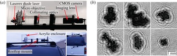
(a) Digital in-line holography deployment used to record snowflake images during the field measurements, showing top: holographic set-up, bottom: mounting on the field vehicle. (b) Samples of in-focus snowflake images after holographic reconstruction.

2.2 Digital holography
Digital in-line holography (DIH) is employed to determine the morphology and size distribution of snowflakes during the deployment. The DIH system, shown in figure 1, consists of a diode laser (Edmund Optics 1 mW; 633 nm), a beam expander (Edmund Optics 20
 $\times$
microscopic objective) and a collimating lens to produce a 50 mm diameter collimated beam. The entire set-up is sealed inside an acrylic container with an opening on the top
 $(6\times 6~\text{cm}^{2})$
allowing snowflakes to fall through the system with minimal interference. To ensure the DIH system imaged only falling snow flakes and not flakes re-suspended in the saltation layer, the DIH system was mounted on the roof of a field vehicle at a height of 2 m as shown in figure 1(a). The field vehicle was located next to the field imaging camera, at a distance of approximately 25 m from the lightsheet. The laser light scattered by the snowflakes interferes with the non-scattered portion of the laser beam to form a hologram, captured on a complementary metal–oxide–semiconductor (CMOS) camera (Pointgrey
 $1920\times 1200~\text{pixel}^{2};5.86~\unicode[STIX]{x03BC}\text{m}~\text{pixel}^{-1}$
) through a 25 mm f/1.4 Fujinon imaging lens at a resolution of
 $16~\unicode[STIX]{x03BC}\text{m}~\text{pixel}^{-1}$
. Due to the limited aperture of the imaging lens, the DIH system yields a cylindrical sampling volume 6 cm in length and 2 cm in diameter. The in-focus snowflake images are obtained through numerical reconstruction and segmentation of the recorded holograms at different distances away from the recording plane (Katz & Sheng Reference Katz and Sheng2010). This method was used in the past to image hydrometeors (Fugal, Schulz & Shaw Reference Fugal, Schulz and Shaw2009) and marine species (Talapatra et al.
Reference Talapatra, Hong, McFarland, Nayak, Zhang, Katz, Sullivan, Twardowski, Rines and Donaghay2013).
Holograms of the snow particles were imaged in multiple recording sets throughout the deployment, with each set containing 1000 frames determined by the camera memory buffer size. For each set, an average of 15 snowflake holograms were acquired. In this fashion, 138 snowflakes were imaged successfully for characterization in a total of nine recordings spread over a duration of 64 min during the deployment. The required snowflake characteristics were extracted by employing a series of image processing techniques. The snowflake holograms were enhanced by subtracting the ensemble-averaged background and reconstructed back into in-focus images. As different portions of the snowflake come into focus at different depths of reconstruction, all the reconstructed holograms are compared to obtain a single minimum intensity image, which is an accurate representation of the two-dimensional projection of the original snowflake. Examples of in-focus images are shown in figure 1(b), wherein one can see the particles (dark region) surrounded by fringe patterns formed by the interference of the scattered beam with the reference beam. Image processing techniques are further applied on this minimum intensity image to extract morphological characteristics such as area, equivalent diameter, eccentricity and shape. A global threshold was applied to select only the snowflakes whose characteristics can be accurately computed.
2.3 Large-scale imaging of snow particles
For illuminating the snowflakes we used a 5 kW searchlight aimed at a curved reflector to generate a lightsheet approximately 30 cm in thickness and gradually increasing in width with the elevation. The lightsheet was approximately aligned with the wind direction at the beginning of the deployment, although the relative angle varied between
 $-5^{\circ }$
and
 $40^{\circ }$
during the observation. Multiple measurements were recorded during the deployment and assessed in post-processing for variability. The measurements shown here had stable wind direction and r.m.s. through the recording. We also verified that the particle velocity statistics did not change significantly when limiting the averages to specific time subwindows. For the data presented here, a CMOS (Sony A7RII, Sony Corp.) 42 megapixel camera acquiring at
 $w120~\text{Hz}$
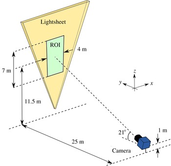
was located at a stand-off distance of 25 m from the lightsheet. The camera imaged the region of interest (ROI) by tilting its axis at
 $21^{\circ }$
from the horizontal to provide a field of view of
 $7\times 4~\text{m}$
as shown in figure 2. A pixel binning of 6 permitted high frame rates reducing the full resolution to
 $720\times 1080~\text{pixel}^{2}$
. We focus on the results from images acquired over a 5 min window, which were processed to extract both two-dimensional Lagrangian particle trajectories and Eulerian velocity fields of the particles in each frame.
Schematic of the field deployment for large-scale imaging of snow particles.

The Eulerian velocity fields were computed using particle image velocimetry (PIV) with an iterative adaptive correlation scheme (Fouras, Lo Jacono & Hourigan Reference Fouras, Lo Jacono and Hourigan2008), a final pass of
 $32\times 32~\text{pixel}^{2}$
and 50 % overlap to give
 $44\times 79$
vectors per frame over 36 000 frames. The rejected outlier vector percentage was under 6.5 % based on the criteria described by Westerweel & Scarano (Reference Westerweel and Scarano2005). At a
 $5.46~\text{mm}~\text{pixel}^{-1}$
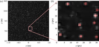
ratio, the vector spacing was 87 mm, compared to a Kolmogorov length scale of 1.3 mm (discussed in § 3.1). Particle tracking velocimetry (PTV) provided Lagrangian particle tracks, extracted using an adaptation of the four-frame best estimate algorithm outlined in Ouellette, Xu & Bodenschatz (Reference Ouellette, Xu and Bodenschatz2006), and using an initial vector estimate interpolated from local PIV vector fields to reduce the particle neighbourhood search to a 3 pixel radius. The tracking algorithm was applied to particle centroids located using Gaussian three-point fitting around those peaks passing a strict maxima criterion on particle intensity, so as to minimize peak-locked statistics. Figure 3 shows a snapshot with a close-up view of snowflake images and their centroid. The average inter-frame particle matching was 60 %, mostly dependent on particles lost due to out-of-plane motion; however the long acquisition window provided well converged statistics. The sampling period of 1/120 s was over 15 times smaller than the Kolmogorov time scale (discussed in § 3.1).
Sample acquisition of snow particles zoomed in on (a) a
 $2\times 2~\text{m}^{2}$
field of view, (b) a
 $32\times 32~\text{pixel}^{2}$
subset of the image corresponding to
 $0.175\times 0.175~\text{m}^{2}$
showing individual snow particles and their centroid locations.

3 Results
3.1 Properties of the atmospheric turbulent flow
The atmospheric conditions during deployment were characterized by moderate wind (average wind speed of
 $3.8~\text{m}~\text{s}^{-1}$
at a height of 127 m), weakly stable thermal conditions and high relative humidity (98 %), typical during snowfalls at night. In particular the bulk Richardson number,
 $Ri_{b}=-|g|\unicode[STIX]{x0394}\overline{\unicode[STIX]{x1D703}}_{v}\unicode[STIX]{x0394}z/(\overline{\unicode[STIX]{x1D703}}_{v}[\unicode[STIX]{x0394}u_{x}^{2}+\unicode[STIX]{x0394}u_{y}^{2}])$
was 0.03 in the area of interest and approaching 0.17 calculated between 7 and 77 m, where
 $\overline{\unicode[STIX]{x1D703}}_{v}$
is the virtual potential temperature. The sonic anemometer at
 $z=10~\text{m}$
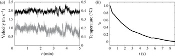
(a height representative for the PTV sampling region) was used to provide a statistical description of the turbulent flow. Records of the velocity and temperature from the meteorological tower are plotted in figure 4(a) and key physical quantities are summarized in table 1. The ratio
 $u_{z}^{\prime }/u_{x}^{\prime }=0.5$
is characteristic of atmospheric boundary layers, where
 $u_{x}^{\prime }$
and
 $u_{z}^{\prime }$
denote the r.m.s. of the horizontal and vertical velocity components, respectively. As customary, we use Taylor hypothesis based on a convection velocity equal to the local mean wind velocity to convert temporal into spatial statistics. The integral length scale,
 $L=4.9~\text{m}$
is calculated from the temporal auto-correlation of the sonic streamwise velocity shown in figure 4(b). According to mixing length theory,
 $L\sim kz=4.1~\text{m}$
,
 $k$
being the von Kármán constant (Townsend Reference Townsend1980), comparable with the above estimate. Because
 $L$
and
 $u^{\prime }$
represents the length and velocity scale of the energy-containing eddies, the turbulent kinetic energy dissipation is approximated as
 $\unicode[STIX]{x1D716}={u^{\prime }}^{3}/L$
, leading to estimates of the Kolmogorov scales
 $\unicode[STIX]{x1D702}=1.3~\text{mm}$
and
 $\unicode[STIX]{x1D70F}_{\unicode[STIX]{x1D702}}=0.13~\text{s}$
, and the Taylor microscale
 $\unicode[STIX]{x1D706}=78~\text{mm}$
.
(a) A 5 min window of the sonic anemometer data showing wind velocity (black line) and air temperature (grey line). (b) Temporal auto-correlation function value,
 $\unicode[STIX]{x1D70C}$
, of the streamwise velocity fluctuations of the 5 min window used to calculate the integral time,
 $\unicode[STIX]{x1D70F}$
and length scale,
 $L$
.

3.2 Size of the snow particles
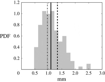
The size of the snowflakes was characterised using digital in-line holography. Figure 5 shows the distribution of the hydrometeor size, denoted by the diameter of a circle of equivalent area. The mean diameter is
 $D_{p}=1.09~\text{mm}$
with a standard deviation in the distribution of 0.45 mm. The DIH images (figure 1) show compact hydrometeor shapes that have an average aspect ratio of 1.39, calculated by least-squares fitting an ellipse to the images. Based on the above particle shape, aspect ratio and size, and considering the air temperature (
 $T=0.1~^{\circ }\text{C}$
) and relative humidity (98 %), the observed hydrometeors fall between the categories of graupel (resulting from the deposition of supercooled water on an ice core) and heavily rimed crystal (Pruppacher & Klett Reference Pruppacher and Klett1997). The appearance, physical properties, and settling velocity are consistent with recent multi-camera images of these types of snow (Garrett & Yuter Reference Garrett and Yuter2014). Granted the snow characteristics, the terms ‘snowflake’ and ‘snow particle’ are used interchangeably throughout the paper.
Histogram of equivalent diameter of snowflakes obtained from DIH measurements during the deployment. The solid line denotes the mean equivalent diameter based on area, the dashed line denotes the mean diameter based on the major axis and the dash-dotted line denotes the mean diameter based on the minor axis.

Estimated quantities from the sonic anemometer. Here
 $U$
denotes the mean streamwise wind velocity,
 $u_{x}^{\prime }$
and
 $u_{z}^{\prime }$
the root mean square (r.m.s.) of the streamwise and vertical velocity components,
 $L$
the integral length scale,
 $\unicode[STIX]{x1D70F}_{L}$
the integral time scale,
 $\unicode[STIX]{x1D716}$
the dissipation rate,
 $\unicode[STIX]{x1D702}$
the Kolmogorov length scale,
 $\unicode[STIX]{x1D70F}_{\unicode[STIX]{x1D702}}$
the Kolmogorov time scale,
 $\unicode[STIX]{x1D706}$
the Taylor microscale and
 $Re_{\unicode[STIX]{x1D706}}$
the turbulence Reynolds number.

(a,c) Spatio-temporal plots of horizontal,
 $u_{x}$
and vertical,
 $u_{z}$
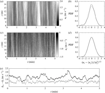
velocities of the inertial particles along the vertical centreline of the imaging plane. (b,d) Distributions of snow particle fluctuating velocities normalized by their standard deviation (solid lines). Dashed line denotes Gaussian distributions. (e) Horizontal
 $\tilde{u} _{x}$
(black line) and vertical
 $\tilde{u} _{z}$
(grey line) velocities obtained averaging the spatio-temporal plots in the
 $z$
-direction.

3.3 Eulerian and Lagrangian description of snow particle kinematics
3.3.1 Snow particle velocities
Figure 6 displays the horizontal and vertical hydrometeor velocities measured from PIV. Spatio-temporal plots extracted along the symmetry line of the ROI are shown, as well as the temporal evolution of vertically averaged horizontal
 $\tilde{u} _{x}$
and vertical
 $\tilde{u} _{z}$
velocity components. Instantaneous vertical profiles show small-scale inhomogeneities, but the stronger fluctuations tend to span the full height of the imaging window. This is consistent with the integral length scale (4.9 m) being of the order of the field of view. Despite large oscillations, the velocity appears stationary in the mean within the 5 min observation. The probability density function (PDF) of the velocity fluctuations show approximately normal distributions of both horizontal and vertical components, which is in accordance with the assumption that snow particles predominantly follow the large-scale turbulence motions, as shown in Toloui et al. (Reference Toloui, Riley, Hong, Howard, Chamorro, Guala and Tucker2014). In this study it was shown that (in snow conditions similar to the ones investigated here) treating the snow flakes as tracers returns mean streamwise velocity, mean shear and turbulent kinetic energy in good agreement with independent air flow measurements obtained from sonic anemometry. Under this hypothesis the vertical profile of the mean horizontal velocity of the snow particles is a good approximation of the wind velocity profile, and indicates a mean shear of
 $S=0.023~\text{s}^{-1}$
within the imaging window. It follows that the ratio of the Kolmogorov time scale to the mean shear time scale is
 $S(\unicode[STIX]{x1D708}/\unicode[STIX]{x1D716})^{1/2}=0.003\ll 1$
, which is the condition proposed by Saddoughi & Veeravalli (Reference Saddoughi and Veeravalli1994) for turbulent shear flows to expect small-scale isotropy. This is important for the following comparison of particle acceleration statistics obtained from DNS and experiments in (nearly) homogeneous isotropic turbulence conditions.
We measure a mean horizontal velocity
 $U=1.24~\text{m}~\text{s}^{-1}$
and a mean vertical (settling) velocity of the snow particles
 $W_{p}=0.86~\text{m}~\text{s}^{-1}$
. The latter is consistent with reported fall speeds of graupel and rimed snow particles (e.g. Locatelli & Hobbs Reference Locatelli and Hobbs1974; Garrett & Yuter Reference Garrett and Yuter2014). The horizontal velocity is close to the wind speed from the sonic anemometer projected into the plane of the measurements. The fall speed is taken as a mean slip velocity, which along with the observed mean diameter
 $D_{p}$
leads to a particle Reynolds number
 $Re_{p}=D_{p}\cdot W_{p}/\unicode[STIX]{x1D708}=70$
.
At this stage, a few considerations are in order on the nature of the particle–turbulence interaction during the present measurements. The turbulence intensity is large (
 $T_{I}=u^{\prime }/U>10\,\%$
), with moderate levels of large-scale anisotropy. The observed snow particles are fairly compact and round, and have dimensions smaller than or equal to the Kolmogorov scale. Their slip velocity Reynolds number is much larger than unity (
 $Re_{p}=70$
) and therefore their drag cannot be approximated by a creeping flow solution. However, because finite-size effects are expected to be negligible, the Stokes number is an appropriate parameter to describe the aerodynamic interaction between the snowflakes and the ambient turbulence. From the particle count and the size of the illuminated volume, the number density is estimated as
 $10^{3}$
particles per
 $\text{m}^{3}$
, which corresponds to a volume fraction of order
 $10^{-7}$
. Assuming a snowflake bulk density of order
 $10^{2}~\text{kg}~\text{m}^{-3}$
(Thompson et al.
Reference Thompson, Field, Rasmussen and Hall2008 as well as our estimates in § 3.4), the solid mass fraction is of order
 $10^{-5}$
. For this number density and mass loading the influence of the particles on the turbulence (two-way coupling) and the inter-particle collisions (four-way coupling) are deemed negligible (Elghobashi Reference Elghobashi1994). Considering the above, the present atmospheric conditions appear as a relevant field-scale setting to (i) test fundamental results obtained in one-way coupled particle-laden turbulence studies, and (ii) extend them towards an unexplored range of particle characteristics and Reynolds number.
3.3.2 Snow particle acceleration and Stokes number
A hallmark feature of inertial particles in turbulence is that their Lagrangian acceleration statistics differ from those of fluid tracers (Toschi & Bodenschatz Reference Toschi and Bodenschatz2009), and the moments of the acceleration PDF are sensitive to the particle Stokes number (Bec et al.
Reference Bec, Biferale, Boffetta, Celani, Cencini, Lanotte, Musacchio and Toschi2006; Salazar & Collins Reference Salazar and Collins2012). Being related to small-scale features of the flow, the dependence of the acceleration with
 $St$
is not expected to be strongly influenced by the specific type of turbulent flow, at least at high Reynolds numbers. For example, the acceleration PDF obtained by Gerashchenko et al. (Reference Gerashchenko, Sharp, Neuscamman and Warhaft2008) for inertial particles in the outer region of a turbulent boundary layer closely matched those obtained in active grid turbulence by Ayyalasomayajula et al. (Reference Ayyalasomayajula, Gylfason, Collins, Bodenschatz and Warhaft2006). We leverage these behaviours and results to estimate the Stokes number of the snowflakes.
(a) Frame-by-frame acceleration (
 $\text{px}/\unicode[STIX]{x0394}t^{2}$
, where
 $\unicode[STIX]{x0394}t=1/120~\text{s}$
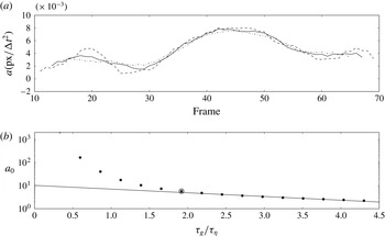
) along a sample particle track evaluated with three different kernel widths: 25 frames (dashed line), 29 frames (solid line) and 33 frames (dash-dotted line). (b) Normalized acceleration variance as a function of kernel width normalized by
 $\unicode[STIX]{x1D70F}_{\unicode[STIX]{x1D702}}$
. The tested kernel widths are indicated by black circles. The final applied kernel width is denoted by the open circle and the solid line represents the exponential fit extrapolated to give an estimate of the normalized acceleration variance
 $a_{0}$
.

We calculate snow particle acceleration following the approach described by Voth et al. (Reference Voth, la Porta, Crawford, Alexander and Bodenschatz2002) and modified by Mordant, Crawford & Bodenschatz (Reference Mordant, Crawford and Bodenschatz2004). A total of
 ${\sim}87\,000$
snow particle trajectories exceeding 32 frames were used to calculate acceleration statistics by convolving them with the normalized second derivative of a Gaussian kernel. The convolution of the derivative of the Gaussian kernel acts both as a numerical derivative and a low-pass filter of the raw data. This is required to reduce the noise associated with particle position uncertainty and to prevent it from contaminating the Lagrangian statistics. The kernel needs to be applied over an appropriate number of consecutive frames, i.e. an appropriate convolution time interval
 $\unicode[STIX]{x1D70F}_{g}$
. For too short intervals particle position uncertainty contaminates the statistics; for too long intervals strong acceleration events are damped by excessive filtering. Figure 7(a) shows an example of frame-by-frame acceleration along a snow particle trajectory calculated using different values of
 $\unicode[STIX]{x1D70F}_{g}$
, and figure 7(b) shows the normalized acceleration variance, defined as
 $a_{0}\equiv \langle {a^{\prime }}^{2}\rangle /(\unicode[STIX]{x1D716}^{3/2}\unicode[STIX]{x1D708}^{-1/2})$
, as a function of
 $\unicode[STIX]{x1D70F}_{g}$
. Following the above-mentioned studies, we chose the smallest
 $\unicode[STIX]{x1D70F}_{g}$
for which the acceleration variance retains an exponential dependency on the interval width. This corresponds to 29 frames, 0.24 s, and is of order
 $\unicode[STIX]{x1D70F}_{\unicode[STIX]{x1D702}}$
(Voth et al.
Reference Voth, la Porta, Crawford, Alexander and Bodenschatz2002; Gerashchenko et al.
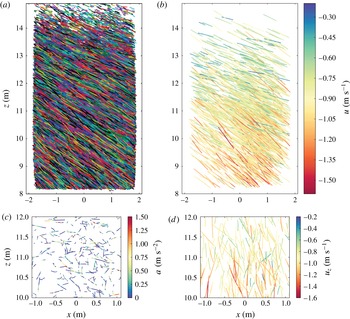
Reference Gerashchenko, Sharp, Neuscamman and Warhaft2008). Finally, the conditional selection on trajectories exceeding 32 frames replaces the statistical weighting based on track length used by Voth et al. (Reference Voth, la Porta, Crawford, Alexander and Bodenschatz2002). Figure 8 displays the (a) ensemble of all trajectories used to calculate acceleration statistics, and (b) highlights the longest 1600 among those. The two bottom panels show a subset of the trajectories in a zoomed ROI of
 $2\times 2~\text{m}^{2}$
with (c) highlighting the acceleration and motion of the particle relative to the mean velocity vector and (d) highlighting the settling motion relative to the streamwise mean velocity.
(a) Snowflake trajectories reconstructed by in situ PTV during 5 min acquisition, with colours used to distinguish the individual tracks. (b) The 1600 longest trajectories colour-coded by instantaneous velocity along each track. (c) Zoomed-in view of 200 trajectories of particles after subtracting the mean settling velocity
 $W_{p}$
and mean horizontal velocity
 $\langle \overline{u}_{x}\rangle$
with colour representing instantaneous acceleration magnitude,
 $a$
. (d) Identical tracks as previous panel with just the mean horizontal velocity subtracted,
 $\langle \overline{u}_{x}\rangle$
, capturing the dynamics of the settling with tracks colour-coded by instantaneous vertical velocity,
 $u_{z}$
.

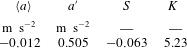
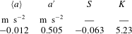
The moments of the in-plane particle acceleration, including skewness
 $S=\langle a^{3}\rangle /\langle a^{\prime 2}\rangle ^{3/2}$
and kurtosis
 $K=\langle a^{4}\rangle /\langle a^{\prime 2}\rangle ^{2}$
, are listed in table 2. The accuracy in calculating the acceleration is affected by the identification of the particle positions and by the choice of the kernel width. The Gaussian fit of the particle intensity profile typically retrieves the centroid location with subpixel accuracy. Applying r.m.s. errors of 0.1, 0.2 and
 $0.5$
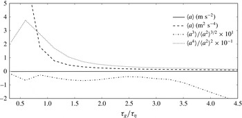
pixels to the particle positions and following a Monte Carlo approach, the acceleration variance changes by 1.2 %, 4.7 % and 29.7 %. The dependence of the acceleration statistics on the kernel width is highlighted in figure 9. In the present study we used
 $\unicode[STIX]{x1D70F}_{g}=1.85\unicode[STIX]{x1D70F}_{\unicode[STIX]{x1D702}}$
(29 frames), which closely matches the
 $1.8\unicode[STIX]{x1D70F}_{\unicode[STIX]{x1D702}}$
interval chosen by Voth et al. (Reference Voth, la Porta, Crawford, Alexander and Bodenschatz2002). Varying
 $\unicode[STIX]{x1D70F}_{g}$
between
 $1.6\unicode[STIX]{x1D70F}_{\unicode[STIX]{x1D702}}$
and
 $2.1\unicode[STIX]{x1D70F}_{\unicode[STIX]{x1D702}}$
(i.e. between 25 and 33 frames) produces changes of 22 % in
 $a^{\prime }$
, 29 % in skewness and 54 % in kurtosis. The mean acceleration, which would be identically zero in isotropic turbulence, is negligibly small irrespective of the kernel width.
Effect of Gaussian filter kernel size normalized by
 $\unicode[STIX]{x1D70F}_{\unicode[STIX]{x1D702}}$
on the statistics of the total acceleration. The kernel width employed in the present study is
 $\unicode[STIX]{x1D70F}_{g}=1.85\unicode[STIX]{x1D70F}_{\unicode[STIX]{x1D702}}$
.

Snow particle acceleration statistics.
 $S$
and
 $K$
indicate skewness and kurtosis respectively.
The normalized acceleration variance is
 $a_{0}=38$
if one uses
 $\unicode[STIX]{x1D70F}_{g}$
(as in Gerashchenko et al.
Reference Gerashchenko, Sharp, Neuscamman and Warhaft2008), while it is equal to
 $65$
if one uses the extrapolated fit to
 $\unicode[STIX]{x1D70F}_{g}=0$
shown in figure 7(b) (as argued by Voth et al.
Reference Voth, la Porta, Crawford, Alexander and Bodenschatz2002). These are significantly larger values than previously reported: for fluid tracers in homogeneous isotropic turbulence at
 $Re_{\unicode[STIX]{x1D706}}\approx 1000$
, DNS showed values in the range 3–4 (Ishihara et al.
Reference Ishihara, Kaneda, Yokokawa, Itakura and Uno2007), while laboratory experiments have found values between 3 and 7 (Voth et al.
Reference Voth, la Porta, Crawford, Alexander and Bodenschatz2002; Gylfason, Ayyalasomayajula & Warhaft Reference Gylfason, Ayyalasomayajula and Warhaft2004); for inertial particles in the outer region of a turbulent boundary layer at
 $Re_{\unicode[STIX]{x1D706}}=240$
, Gerashchenko et al. (Reference Gerashchenko, Sharp, Neuscamman and Warhaft2008) found
 $a_{0}\approx 4$
. This large
 $a_{0}$
can be attributed to multiple factors. Firstly, atmospheric flows are likely to be more intermittent than the turbulence generated in the laboratory or by DNS. Intermittency plays a key role in determining the acceleration variance, and in fact lies at the root of
 $a_{0}$
being higher than 1 as predicted by Gaussian models (see discussions in Shaw & Oncley Reference Shaw and Oncley2001; Voth et al.
Reference Voth, la Porta, Crawford, Alexander and Bodenschatz2002). Indeed, Gulitski et al. (Reference Gulitski, Kholmyansky, Kinzelbach, Lüthi, Tsinober and Yorish2007) measured values of
 $a_{0}$
up to
 ${\sim}15$
in the atmospheric surface layer. Secondly, recent simulations of Ireland, Bragg & Collins (Reference Ireland, Bragg and Collins2016b
) indicate that settling inertial particles experience different regions of the turbulence during their downward drift, a mechanism they refer to as ‘gravitational trajectory effect’. For particles of
 $St=O(1)$
this largely offsets the filtering effect due to particle inertia, and results in a multi-fold increase in acceleration variance compared to fluid tracers.
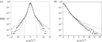
Figure 10 shows the acceleration PDF (normalized by the
 $a^{\prime }$
) for the horizontal and vertical components, as well as for the in-plane acceleration. The PDF of the in-plane acceleration is fairly symmetric, while the horizontal and vertical components have somewhat positive (
 $S=0.094$
) and negative skewness (
 $S=-0.22$
), respectively. This asymmetry is possibly a consequence of gravity, although the exact mechanism is not clear and deserves further investigation. Another potential explanation is mean shear: Gerashchenko et al. (Reference Gerashchenko, Sharp, Neuscamman and Warhaft2008) measured similar levels of skewness for particles at
 $St=0.07$
in the outer region of a turbulent boundary layer, although in their case the sign of the skewness changed with wall distance.
(a) PDFs of normalized horizontal (open circles) and vertical (filled circles) accelerations of snow particles, compared to
 $St=0$
from Mordant et al. (Reference Mordant, Crawford and Bodenschatz2004) (small filled circles) and a Gaussian distribution (dashed line). (b) PDF of in-plane acceleration magnitude of the snow particles (black triangles), along with the results of Mordant et al. (Reference Mordant, Crawford and Bodenschatz2004) (small filled circles), Ayyalasomayajula et al. (Reference Ayyalasomayajula, Gylfason, Collins, Bodenschatz and Warhaft2006) (
 $St=0.09$
,
 $\times$
;
 $St=0.15$
,
 $+$
) and Bec et al. (Reference Bec, Biferale, Boffetta, Celani, Cencini, Lanotte, Musacchio and Toschi2006) (
 $St=0.16$
, solid line;
 $St=0.37$
, dash-dotted line).

The acceleration distributions in figure 10 show the typical stretched exponential shape, with tails extending much further than in the Gaussian distribution of the same variance (also shown for comparison). The long tails are the most remarkable aspect of the acceleration PDFs. For the following analysis it is useful to reason on how the snowflake acceleration distribution may be influenced by the turbulence properties. This is not a settled problem, largely due to the difficulty in observing and simulating high Reynolds number flows. For fluid tracers in isotropic turbulence, Voth et al. (Reference Voth, la Porta, Crawford, Alexander and Bodenschatz2002) reports a dependence of the acceleration kurtosis on
 $Re_{\unicode[STIX]{x1D706}}$
that seems to point to an asymptotic behaviour, but the experimental uncertainties do not allow firm conclusions. The DNS of Ishihara et al. (Reference Ishihara, Kaneda, Yokokawa, Itakura and Uno2007) instead suggests that the acceleration kurtosis scales with
 $Re_{\unicode[STIX]{x1D706}}$
with an exponent close to unity (consistently with the refined similarity hypothesis (Kolmogorov Reference Kolmogorov1962)). The DNS, however, is found to systematically overestimate the accelerations compared with experiments, the reasons for which are unclear. For inertial particles in turbulence the extension of the tails in the acceleration PDF appears to have a significantly stronger dependence on the Stokes number than on the Reynolds number of the turbulent flow, as suggested by the fact that distributions from the simulations of Bec et al. (Reference Bec, Biferale, Boffetta, Celani, Cencini, Lanotte, Musacchio and Toschi2006)
 $Re_{\unicode[STIX]{x1D706}}=185$
are relatively close to the measurements of Ayyalasomayajula et al. (Reference Ayyalasomayajula, Gylfason, Collins, Bodenschatz and Warhaft2006) at
 $Re_{\unicode[STIX]{x1D706}}=250$
. Studies at Reynolds numbers comparable to the present case are scarce, but the large-scale DNS of Ireland et al. (Reference Ireland, Bragg and Collins2016b
) show only small changes of the kurtosis of inertial particle accelerations above
 $Re_{\unicode[STIX]{x1D706}}=398$
. Although there is scatter in the experimental data, the acceleration PDF we measure for the snow particles falls in the range spanned by the
 $St=0.09$
case of Ayyalasomayajula et al. (Reference Ayyalasomayajula, Gylfason, Collins, Bodenschatz and Warhaft2006) and the
 $St=0.37$
case of Bec et al. (Reference Bec, Biferale, Boffetta, Celani, Cencini, Lanotte, Musacchio and Toschi2006). Therefore, assuming the differences between the turbulence properties in these studies and in the present flow have a secondary effect on the PDF tails, we use the match of acceleration PDFs between laboratory studies and our measurements (shown in figure 10) to infer a snow particle Stokes number in the range
 $St=0.09{-}0.37$
. Accounting for the differences between our atmospheric flow and those in previous studies, one may expect differences in the acceleration PDF, and as such this is necessarily an estimate. However, as it will be shown, it is consistent with the physical properties of the hydrometeors. Note that at this stage, an independent measure of the Stokes number would require a model for the snow flake drag (not a creeping flow solution) and an estimate of the snow flake density, which are both non-trivial to obtain accurately. Hence, the decision to use particle acceleration to estimate the Stokes number first. From the particle Stokes number and the Kolmogorov time scale, it follows that the aerodynamic response time of the observed hydrometeors
 $$\begin{eqnarray}\unicode[STIX]{x1D70F}_{p}=V_{t}/g=St\cdot \unicode[STIX]{x1D70F}_{\unicode[STIX]{x1D702}}\end{eqnarray}$$
is in the range 12–48 ms.
3.4 Estimate of snowflake bulk density
Typically in atmospheric science the settling velocity of the snow particles
 $W_{p}$
is an unknown which has to be determined from estimates of the hydrometeor size and density. The density of frozen hydrometeors can vary in the wide range
 $10{-}910~\text{kg}~\text{m}^{-3}$
(Locatelli & Hobbs Reference Locatelli and Hobbs1974; Pruppacher & Klett Reference Pruppacher and Klett1997; Heymsfield et al.
Reference Heymsfield, Bansemer, Schmitt, Twohy and Poellot2004), but for snowflakes
 ${\sim}1$
mm in size a wealth of field studies indicate values of
 ${\sim}100~\text{kg}~\text{m}^{-3}$
, as apparent from the collection of studies summarized by Thompson et al. (Reference Thompson, Field, Rasmussen and Hall2008). To calculate the settling velocity
 $W_{p}$
, empirical expressions are often used which relate the particle Reynolds number
 $Re_{p}$
and the drag coefficient
 $C_{D}$
(Böhm Reference Böhm1989; Heymsfield & Westbrook Reference Heymsfield and Westbrook2010). The first step is to calculate the so-called Best number
 $X=C_{D}{Re_{p}}^{2}$
, which is independent of settling velocity. Indeed from the balance of drag and gravity on a snowflake falling at terminal velocity, one has:
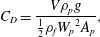 $$\begin{eqnarray}C_{D}=\frac{V\unicode[STIX]{x1D70C}_{p}g}{\displaystyle {\textstyle \frac{1}{2}}\unicode[STIX]{x1D70C}_{f}{W_{p}}^{2}A_{p}},\end{eqnarray}$$
where
 $A_{p}$
is the projected hydrometeor area normal to the fall motion and
 $V$
is its volume. The Best number is then:
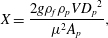 $$\begin{eqnarray}X=\frac{2g\unicode[STIX]{x1D70C}_{f}\unicode[STIX]{x1D70C}_{p}V{D_{p}}^{2}}{\unicode[STIX]{x1D707}^{2}A_{p}},\end{eqnarray}$$
which can be obtained from measured or assumed hydrometeor properties. The vast literature on settling of frozen hydrometeors has produced empirical
 $Re_{p}{-}X$
relations based on both laboratory and field observations. From those one can calculate
 $Re_{p}$
and therefore the sought fall speed
 $W_{p}$
. In the present case we directly measure
 $W_{p}$
and therefore we can invert the procedure to estimate the snow particle density. We employ the widely used expression derived by Böhm (Reference Böhm1989):
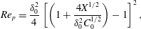 $$\begin{eqnarray}Re_{p}=\frac{\unicode[STIX]{x1D6FF}_{0}^{2}}{4}\left[\left(1+\frac{4X^{1/2}}{\unicode[STIX]{x1D6FF}_{0}^{2}C_{0}^{1/2}}\right)-1\right]^{2},\end{eqnarray}$$
with values of the pressure drag coefficient
 $C_{0}=0.6$
and surface roughness constant
 $\unicode[STIX]{x1D6FF}_{0}=5.83$
which were found to provide good agreement with observations of falling ice and graupel (Mitchell Reference Mitchell1996). For the present value of
 $Re_{p}=70$
, equation (3.4) yields
 $X=8465$
and so
 $C_{D}=1.76$
. From (3.2) and using the measured effective diameter, we obtain
 $\unicode[STIX]{x1D70C}_{p}=118~\text{kg}~\text{m}^{-3}$
. This is in good agreement with the aircraft measurements of Heymsfield et al. (Reference Heymsfield, Bansemer, Schmitt, Twohy and Poellot2004) and the ground measurements of Brandes et al. (Reference Brandes, Ikeda, Zhang, Schönhuber and Rasmussen2007) for the same hydrometeor class and size range as in our case. The former used a combination of spectrometry and a counterflow impactor, while the latter used a video disdrometer.
One could also infer the particle density from the estimate of the aerodynamic response time and the Stokesian expression of
 $\unicode[STIX]{x1D70F}_{p}$
corrected for finite particle Reynolds number by Schiller & Naumann (see Clift, Grace & Weber Reference Clift, Grace and Weber2005):
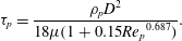 $$\begin{eqnarray}\unicode[STIX]{x1D70F}_{p}=\frac{\unicode[STIX]{x1D70C}_{p}D^{2}}{18\unicode[STIX]{x1D707}(1+0.15{Re_{p}}^{0.687})}.\end{eqnarray}$$
Schiller & Naumann’s formula was obtained in steady and uniform flow around a perfectly spherical particle – assumptions which are clearly violated here. Although it is often used in point-particle simulations, it has not been adopted in previous snow settling studies. Indeed, given the range of
 $\unicode[STIX]{x1D70F}_{p}=12{-}48~\text{ms}$
, equation (3.5) would return a density of
 $11{-}44~\text{kg}~\text{m}^{-3}$
. This is at the low end of the reported range for frozen hydrometeors and rather consistent with measurement of fresh snow density (e.g. Clifton et al.
Reference Clifton, Manes, Rüedi, Guala and Lehning2008), but well below what was observed for graupel and heavily rimed crystals. On the other hand the
 $Re{-}X$
relation, which returns much more realistic density values, was obtained from laboratory and field experiments on actual frozen hydrometeors (or models thereof), incorporates the effects of realistic morphology and environmental conditions, and therefore is deemed more appropriate for snowfall.
3.5 Turbulence-enhanced settling velocity
The estimate of the hydrometeor aerodynamic response time allows us to directly evaluate their still-air terminal velocity,
 $V_{t}=\unicode[STIX]{x1D70F}_{p}\cdot g$
. Given the range of
 $\unicode[STIX]{x1D70F}_{p}$
deduced from the acceleration PDF, one finds
 $V_{t}$
ranging between
 $0.12{-}0.47~\text{m}~\text{s}^{-1}$
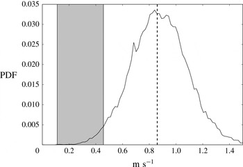
, which is several times smaller than the observed mean settling velocity. The multi-fold velocity enhancement with respect to quiescent fluid conditions is displayed in figure 11, showing the still-air settling velocity range and the observed probability distribution of the snow particle vertical velocity from PTV.
Comparison of the measured distribution (solid line) and average (dashed line) of settling velocity
 $W_{p}$
against the predicted range of still-air terminal velocity
 $V_{t}$
(grey region).

Such a fall speed enhancement is interpreted as an effect of the particle–turbulence interaction. As mentioned in the introduction, the majority of previous numerical and experimental studies found that turbulence significantly enhances the settling velocity of small inertial particles by means of the preferential sweeping mechanism (Wang & Maxey Reference Wang and Maxey1993; Yang & Lei Reference Yang and Lei1998; Aliseda et al.
Reference Aliseda, Cartellier, Hainaux and Lasheras2002; Yang & Shy Reference Yang and Shy2005; Dejoan & Monchaux Reference Dejoan and Monchaux2013; Good et al.
Reference Good, Ireland, Bewley, Bodenschatz, Collins and Warhaft2014; Ireland, Bragg & Collins Reference Ireland, Bragg and Collins2016a
; Rosa et al.
Reference Rosa, Parishani, Ayala and Wang2016). In particular, the measurements of Aliseda et al. (Reference Aliseda, Cartellier, Hainaux and Lasheras2002) and Good et al. (Reference Good, Ireland, Bewley, Bodenschatz, Collins and Warhaft2014) showed that droplets with
 $St$
of order unity falling in air turbulence can reach settling velocities two to three times larger than in still air. Those experiments were conducted at Reynolds numbers one order of magnitude lower than the present one. Numerical studies have also been limited in Reynolds numbers and typically reported maximum settling enhancements of 30 % to 80 %. Recent simulations covering wide parameter ranges suggest that settling enhancement is indeed stronger for higher turbulent dissipation rates (Ayala et al.
Reference Ayala, Rosa, Wang and Grabowski2008; Rosa et al.
Reference Rosa, Parishani, Ayala and Wang2016) and larger
 $Re_{\unicode[STIX]{x1D706}}$
(Ireland et al.
Reference Ireland, Bragg and Collins2016a
).
Because of the complexity of the particle–turbulence interaction, there are multiple candidates for the role of dominant velocity scale and temporal scale determining the settling enhancement. After Wang & Maxey (Reference Wang and Maxey1993),
 $\unicode[STIX]{x1D70F}_{\unicode[STIX]{x1D702}}$
is usually considered the appropriate time scale (hence the usual definition of the Stokes number), while both
 $u^{\prime }$
and
 $u_{\unicode[STIX]{x1D702}}$
have been proposed as characteristic velocity scale. Wang & Maxey commented that the low-vorticity regions where particles accumulate resemble the large-scale flow features characterized by
 $u^{\prime }$
, and Yang & Lei (Reference Yang and Lei1998) argued that
 $u^{\prime }$
is the velocity scale that determines the drag on the settling particles, which is a crucial element for the increase of the settling rate. Still the issue has remained open, partly because the scale separation in numerical and experimental studies has been limited, with
 $u^{\prime }/u_{\unicode[STIX]{x1D702}}$
at most approximately 7. We can use the present high Reynolds number case to gain insight on this question using the following argument. When gravity is acting, the particle–turbulence interaction is described not only by
 $St$
but also by the settling parameter
 $Sv$
, i.e. the ratio of the settling velocity to either the small-scale velocity,
 $Sv_{\unicode[STIX]{x1D702}}=V_{t}/u_{\unicode[STIX]{x1D702}}$
, or the large-scale velocity,
 $Sv_{L}=V_{t}/u^{\prime }$
. Depending on whether
 $u_{\unicode[STIX]{x1D702}}$
or
 $u^{\prime }$
is the characteristic velocity scale for preferential sweeping, one expects maximum settling velocity enhancement when either
 $Sv_{\unicode[STIX]{x1D702}}\approx 1$
or
 $Sv_{L}\approx 1$
(which is analogous to the condition of both Stokes and Froude number,
 $Fr=StSv^{2}$
being of order unity, see Davila & Hunt (Reference Davila and Hunt2001), Rosa et al. (Reference Rosa, Parishani, Ayala and Wang2016)). In our field experiment there is substantial scale separation, with
 $Re_{\unicode[STIX]{x1D706}}\approx 1000$
,
 $L/\unicode[STIX]{x1D702}\approx 3750$
and
 $u^{\prime }/u_{\unicode[STIX]{x1D702}}\approx 16$
. From the estimated range for
 $V_{t}$
, we have
 $Sv_{\unicode[STIX]{x1D702}}=11{-}47$
and
 $Sv_{L}=0.7{-}2.9$
. In other words the observed snow particles, whose fall speed is greatly increased by the turbulence, have a still-air settling velocity much larger than the Kolmogorov velocity but of the same order as the large-eddy velocity. This is consistent with the proposal that
 $u^{\prime }$
is indeed the appropriate velocity scale associated with turbulence-enhanced settling. One may argue that much lighter snow particles (with
 $Sv_{\unicode[STIX]{x1D702}}=O(1)$
and
 $Sv_{L}\ll 1$
) could display even more strongly enhanced settling. This however seems unrealistic, at least in the present conditions, since such particles would have
 $St_{\unicode[STIX]{x1D702}}\ll 1$
and therefore would be unlikely to experience preferential sweeping.
The present results may also help to shed some light on longstanding questions on the relationship between snowflake size, density and fall speed. In fact, these results support the proposition that the physical properties of hydrometeors can only partially explain the large scatter of snow settling velocity reported in the literature. This is underscored by a recent study by Garrett & Yuter (Reference Garrett and Yuter2014), reporting on simultaneously measured snowflake size, morphology and fall speed using a multi-angle camera system. They noted that unrealistic density estimates are obtained if it is assumed that the settling velocity is equal to the terminal velocity of the particles in quiescent air. The present results support the hypothesis that turbulence has a dominant role in determining not only the variance but also the mean of the snowflake fall speed.
4 Conclusions and discussions
We have presented results of the first direct observation of snowflake trajectories in atmospheric turbulence. We characterized the air flow, the hydrometeor properties and their motion using a combination of meteorological tower data, digital in-line holography and large-scale particle imaging. Although the flow was an atmospheric surface layer on a flat field site, the level of shear in the region of interest was low enough to expect homogeneous isotropic conditions at the small scales. The hydrometeors, classified as graupel or heavily rimed crystals, were fairly compact and with sizes of the order of the Kolmogorov length. Despite the non-canonical aspects of the natural precipitation (e.g. non-sphericity and polydispersity of the dispersed phase and large-scale anisotropy of the environmental turbulence), the snowflakes motion exhibits signature features described by laboratory experiments and numerical simulations investigating inertial particles in turbulence. The snow particle velocity fluctuations display a Gaussian distribution, while the acceleration distribution has stretched exponential tails. By comparing with previous studies of particle acceleration in homogeneous turbulence, and assuming that the specific features of the turbulence play a limited role at this high Reynolds number, we deduce that the observed snowflakes have a Stokes number (based on the Kolmogorov time scale) between 0.09 and 0.37. Consistent with previous studies at much lower Reynolds numbers, the mean settling velocity is found to be much greater than the expected still-air fall speed. Because the turbulent flow was stationary during the observation window, the increase in settling velocity is deemed to be caused by the turbulent motion rather than by oscillations in wind direction. If our assumptions are correct, one is led to conclude that the preferential sweeping mechanism described by Wang & Maxey (Reference Wang and Maxey1993) is active and plays a key role in determining the fall speed of snowflakes in atmospheric turbulence. The observed particles have
 $St=O(0.1)$
and
 $Sv_{L}=O(1)$
, suggesting that
 $u^{\prime }$
is the dominant velocity scale in the process of settling enhancement. These considerations are specific to the type of compact frozen hydrometeors we observed. It is likely that snowflakes of different size, bulk density and shape will experience different dynamics, depending on their coupling with spatio-temporal scales of the turbulence.
We remark that the accuracy in atmospheric field measurements is limited by the very nature of the environment. Although we attempt to estimate the uncertainties, precision error bars are difficult to calculate especially for quantities that are inherently challenging to measure, such as turbulence dissipation and particle acceleration. Therefore possible biases can certainly affect the quantitative results. Given the apparent trends highlighted above, the qualitative conclusions are not expected to be overshadowed by measurement uncertainty. However, we acknowledge that the quantification of enhanced settling are based on the assumption that the observed acceleration tails and the consequent estimate of the Stokes number are not majorly affected by gravity, by the specific value of the turbulence Reynolds number nor by large-scale anisotropy. While suggesting caution in interpreting the present data, the above assumption points to specific questions deserving of further investigation, essential to bridging the gap between canonical studies and real precipitation phenomena.
To the best of our knowledge, this is the first time that evidence of settling enhancement by turbulence is found via direct measurements of natural precipitation. The effect of preferential sweeping, and in general the impact of turbulence on the fall speed, can be especially important for snow, for which neither the size nor the bulk density are known a priori and assumptions on the terminal velocity are often used. The results suggest that settling modification by turbulence is the likely cause of inconsistencies among different field studies, and that air turbulence should be incorporated in more accurate size–velocity correlations. Moreover, during intense snowfall events the effect on snowflake acceleration may crucially affects collision probability and hence the evolution of hydrometeor size distribution. Although this was not the case in the investigated conditions, which presented a relatively low number density of hydrometeors, the snowflake size evolution may be profoundly impacted by the turbulence characteristics in strong precipitation events. Given the typical scales of atmospheric turbulence, conditions similar to the ones encountered here could be met by various types of snow and even by other classes of hydrometeors. Further field observations are warranted to investigate other forms of precipitation and different regions of the parameter space.
Finally, the estimate of the aerodynamic response time of the snow particles opens interesting possibilities for imaging snowflakes to quantitatively investigate atmospheric turbulence. Large-scale flow imaging in the atmospheric boundary layer and in the wake of a wind turbine were recently obtained using snowflakes by Hong et al. (Reference Hong, Toloui, Chamorro, Guala, Howard, Riley, Tucker and Sotiropoulos2014) and Toloui et al. (Reference Toloui, Riley, Hong, Howard, Chamorro, Guala and Tucker2014), respectively. Following the reasoning of Toloui et al. (Reference Toloui, Riley, Hong, Howard, Chamorro, Guala and Tucker2014), if micrometre-sized oil droplets (with
 $\unicode[STIX]{x1D70F}_{p}$
of order
 $10^{-5}~\text{s}$
) can follow temporal fluctuations of time scales down to 1 ms (Melling Reference Melling1997), then the observed hydrometeors (with
 $\unicode[STIX]{x1D70F}_{p}$
of order
 $10^{-2}~\text{s}$
) can follow fluctuations down to 1 s. Taking
 $u^{\prime }=0.16~\text{m}~\text{s}^{-1}$
as the relevant velocity scale in the present case, this translates into traceable turbulent length scales of
 $16~\text{cm}$
. Considering the achievable field of view and the size of the energy-containing eddies in the atmospheric boundary layer, this would be an adequate level of spatial resolution to study coherent structures over a wide range of scales.