1. Introduction
Tax evasion is defined as the illicit and deliberate actions undertaken by individuals to reduce their legally owed tax liabilities. Such actions encompass underreporting income, overstating deductions, exemptions, or credits, engaging in barter transactions, or making intentional errors, such as failing to file correct tax returns. These unlawful behaviors primarily fall under the purview of individual income taxation.Footnote 1 It is crucial to underscore the pivotal role that tax evasion plays in the foundational aspects of public economics and macroeconomics. In particular, tax evasion introduces distortions in resource allocation, as individuals modify their behavior to evade taxes, influencing decisions related to work hours, occupational choices, and investment strategies. The existence of tax evasion necessitates governmental expenditures to detect non-compliance, assess its magnitude, and penalize those involved. In addition, non-compliance results in unpredictable shifts in income distribution. This raises several questions: Does the presence of tax evasion exacerbate wealth inequality? Furthermore, can a higher penalty levied on underreported income ameliorate this inequality?
To answer these questions, we consider a heterogeneous-agent economy where households are exposed to uninsured idiosyncratic shocks but subject to incomplete markets and ad hoc borrowing limits. Due to uninsured idiosyncratic shocks, the general equilibrium outcome of heterogeneous-agent incomplete-markets models features inequalities in wealth and consumption. This framework enables us to examine the role of income taxation for workers who encounter financial market imperfections by endogenizing the decision-making process behind tax evasion and encompassing both the decision to evade taxes and the degree of tax compliance. We inquire whether the decision to engage in tax evasion can mitigate the repercussions of market imperfections on the economy. In addition, we examine the effects of the income tax rate on tax evasion and explore how fiscal instruments affect tax evasion by altering the number of financially constrained individuals in this heterogeneous-agent incomplete-markets economy.
Over 50 years ago, Allingham and Sandmo (Reference Allingham and Sandmo1972) formally analyzed the relationship between fiscal instruments (e.g., income tax rates, audit rates, and penalties) and tax evasion.Footnote 2 They found that with decreasing absolute risk aversion, a higher tax rate could either increase or decrease evasion, depending on whether the penalty is levied on undeclared income.Footnote 3
Yitzhaki (Reference Yitzhaki1974) modified this model, arguing that when the substitution effect vanishes, higher tax rates lead to greater compliance due to the income effect. However, empirical studies, such as Clotfelter (Reference Clotfelter1983); Slemrod (Reference Slemrod1985); Alm et al. (Reference Alm, Bahl and Murray1990); Lang et al. (Reference Lang, Nöhrbaß and Stahl1997); Pommerehne and Weck-Hannemann (Reference Pommerehne and Weck-Hannemann1996), which examine taxpayers in the U.S., Jamaica, Germany, and Switzerland, consistently find a positive correlation between tax rates and evasion. Feinstein (Reference Feinstein1991) reported mixed results, while Fisman and Wei (Reference Fisman and Wei2004) showed that the relationship varies with tax magnitude in Chinese import data. These contradictions give rise to the so-called Yitzhaki puzzle.
Two main approaches have emerged to address the Yitzhaki puzzle. The first explores alternative static models of tax evasion. Gordon (Reference Gordon1989) incorporated social norms, showing how they can create a positive link between tax rates and evasion. In contrast, Yaniv (Reference Yaniv1999) argued that rising tax advances incentivize compliance. Lee (Reference Lee2001) suggested that taxpayers invest in risk-mitigation strategies, ultimately increasing evasion. Panadés (Reference Panadés2004) highlighted how the externality of others’ reported income could amplify underreporting as tax rates rise. Lastly, Dhami and Al-Nowaihi (Reference Dhami and Al-Nowaihi2007), using prospect theory, demonstrated that higher tax rates induce risk-seeking behavior, raising evasion.
The second approach to addressing the Yitzhaki puzzle incorporates tax evasion into dynamic models. Lin and Yang (Reference Lin and Yang2001) extended the portfolio choice model, showing that while higher tax rates suppress evasion in static settings, they promote it dynamically. Chen (Reference Chen2003) established a theoretical negative relationship between tax compliance and tax rates in an endogenous growth model. Caballé and Panadés (Reference Caballé and Panadés2007) found that in a multi-period economy, unreported income decreases with tax rates when fines apply to evaded taxes but increases when penalties are proportional to undeclared income. Similarly, Lee (Reference Lee2015) showed that under a tax prepayment system, a higher tax rate raises evasion if penalties target undeclared income, while its effect depends on income level when penalties apply to evaded taxes.
Our paper contributes to the existing literature by examining a heterogeneous-agent economy where households face uninsured idiosyncratic shocks and are subject to incomplete markets and ad hoc borrowing limits, factors often overlooked in the literature on the Yitzhaki puzzle. Specifically, we integrate tax evasion into the frameworks established by Huggett (Reference Huggett1993), Aiyagari (Reference Aiyagari1994), and notably Wen (Reference Wen2015), to gain new implications from the previous research in the following respects.
Firstly, most static models of the Yitzhaki puzzle overlook the role of borrowing constraints in tax evasion. However, empirical evidence suggests that firms in financially developed economies report a higher share of sales to tax authorities (Beck et al. Reference Beck, Chen and Ma2014; Dabla-Norris et al. Reference Dabla-Norris, Gradstein and Inchauste2008). Taxpayers may also evade taxes as a savings mechanism, even in the presence of strict enforcement (Andreoni Reference Andreoni1992). Moreover, several studies indicate a negative relationship between financial frictions and the size of the informal sector (Capasso and Jappelli Reference Capasso and Jappelli2013; Bittencourt et al. Reference Bittencourt, Gupta and Stander2014; Alm et al. Reference Alm, Liu and Zhang2019; Chiarini et al. Reference Chiarini, Ferrara and Marzano2020; Guo and Hung Reference Guo and Hung2020).
Secondly, while dynamic models of the Yitzhaki puzzle typically assume a representative agent,Footnote 4 our model departs from this assumption by introducing heterogeneous taxpayers. Notably, our model differs from Guo and Hung (Reference Guo and Hung2020) in two key respects: (i) it features infinitely-lived households with idiosyncratic preference shocks, whereas Guo and Hung (Reference Guo and Hung2020) focus on firm-specific borrowing constraints, and (ii) we examine how fiscal policies influence the proportion of financially constrained individuals, while they analyze the impact of tax audits on financially constrained firms.
In this framework, we analytically explore the trade-off between aggregate and individual allocative efficiency in a setting where tax evasion does not lead to wealth redistribution. Our model extends the approach of Chien and Wen (Reference Chien and Wen2022) by incorporating tax evasion choices. It is grounded in the framework of Aiyagari (Reference Aiyagari1994), but introduces two important modifications: (i) individuals face idiosyncratic shocks to the marginal utility of consumption, and (ii) their preferences are quasi-linear. This specific preference structure, as noted by Chien and Wen (Reference Chien and Wen2022), eliminates wealth-redistribution effects, enabling us to derive the competitive equilibrium in closed form. Unlike the Aiyagari model, our framework results in a degenerate wealth distribution among individuals, further excluding redistribution effects related to tax evasion. In the absence of such effects, tax evasion in the steady state enhances individuals’ self-insurance, which in turn improves aggregate allocative efficiency. This framework allows us to more clearly highlight the efficiency implications of tax evasion.
Our research closely relates to Maffezzoli (Reference Maffezzoli2011), Kotsogiannis and Mateos-Planas (Reference Kotsogiannis and Mateos-Planas2019), Di Nola et al. (Reference Di Nola, Kocharkov, Scholl and Tkhir2021), Fernandez-Bastidas (Reference Fernandez-Bastidas2023), and Rotberg and Steinberg (Reference Rotberg and Steinberg2024). Maffezzoli (Reference Maffezzoli2011) developed a dynamic general equilibrium Bewley-Huggett-Aiyagari model that endogenizes tax evasion and income heterogeneity, focusing on capital income as the primary misreportable source. Kotsogiannis and Mateos-Planas (Reference Kotsogiannis and Mateos-Planas2019) examined income tax evasion in an incomplete-markets framework, treating evasion as a form of contingent debt, emphasizing risk and credit constraints. Di Nola et al. (Reference Di Nola, Kocharkov, Scholl and Tkhir2021) studied self-employment tax evasion in a dynamic setting, highlighting its role in easing credit constraints while reducing firm productivity. Fernandez-Bastidas (Reference Fernandez-Bastidas2023) explored the effects of switching from progressive to proportional taxation, with a focus on entrepreneurial tax evasion. Finally, Rotberg and Steinberg (Reference Rotberg and Steinberg2024) analyzed offshore tax evasion in response to capital taxation, assessing its implications for wealth inequality, tax revenue, and welfare.
Kotsogiannis and Mateos-Planas (Reference Kotsogiannis and Mateos-Planas2019) Maffezzoli (Reference Maffezzoli2011), Di Nola et al. (Reference Di Nola, Kocharkov, Scholl and Tkhir2021), Fernandez-Bastidas (Reference Fernandez-Bastidas2023), and Rotberg and Steinberg (Reference Rotberg and Steinberg2024) quantitatively analyzed the effects of tax progressivity on evasion, welfare, and inequality. Di Nola et al. (Reference Di Nola, Kocharkov, Scholl and Tkhir2021) emphasized the role of tax evasion in alleviating credit constraints, while Kotsogiannis and Mateos-Planas (Reference Kotsogiannis and Mateos-Planas2019), Maffezzoli (Reference Maffezzoli2011), Fernandez-Bastidas (Reference Fernandez-Bastidas2023), and Rotberg and Steinberg (Reference Rotberg and Steinberg2024) examined how tax reforms influence evasion, inequality, revenue, and welfare. Kotsogiannis and Mateos-Planas (Reference Kotsogiannis and Mateos-Planas2019) found that shifting from progressive to flat tax schedules had a limited effect on evasion due to increased household savings. Similarly, Maffezzoli (Reference Maffezzoli2011) and Fernandez-Bastidas (Reference Fernandez-Bastidas2023) concluded that transitioning to proportional taxation reduces evasion and raises output or revenue, though with heterogeneous effects on inequality and welfare. Lastly, Rotberg and Steinberg (Reference Rotberg and Steinberg2024) demonstrated that tax reforms absent evasion significantly boost welfare and revenue, whereas accounting for evasion reverses these gains, leading to marginal revenue increases, higher inequality, and welfare losses. While these studies provide valuable insights through well-calibrated quantitative models, they do not always explicitly disentangle the mechanisms driving macroeconomic interactions in a general equilibrium setting. In this regard, our work complements theirs by offering a theoretical perspective within a Bewley-Huggett-Aiyagari framework.
Unlike Kotsogiannis and Mateos-Planas (Reference Kotsogiannis and Mateos-Planas2019) and Maffezzoli (Reference Maffezzoli2011), our study focuses on tax evasion as a strategy used by financially constrained households to mitigate idiosyncratic shocks in the presence of incomplete markets and borrowing constraints. Specifically, we highlight tax evasion’s role in enhancing aggregate allocative efficiency, an effect also found numerically in Di Nola et al. (Reference Di Nola, Kocharkov, Scholl and Tkhir2021). Moreover, our findings align with Di Nola et al. (Reference Di Nola, Kocharkov, Scholl and Tkhir2021) in showing that while increasing penalty rates initially improves welfare, excessive penalties ultimately lead to welfare losses. However, whereas their analysis incorporates self-employment, we numerically demonstrate the existence of an optimal penalty rate even without accounting for self-employment.
Beyond these parallels, our theoretical framework advances the literature by identifying three distinct effects of a labor income tax rate on underreported income: the direct effect, the threshold effect, and the income effect. These effects clarify the conditions under which the Yitzhaki puzzle arises. Departing from Fernandez-Bastidas (Reference Fernandez-Bastidas2023), which centers on entrepreneurship, our study focuses on household behavior. Furthermore, while Rotberg and Steinberg (Reference Rotberg and Steinberg2024) found that tax evasion mitigates the macroeconomic consequences of higher capital and wealth taxes, their work primarily examines capital tax evasion and entrepreneurial opportunities in differentiated goods production, distinguishing it from our analysis.
We outline our main theoretical findings as follows. Firstly, tax evasion acts as a strategy employed by financially constrained households to mitigate the adverse impact of financial market imperfections on their situations. Despite the associated uncertainty, tax evasion functions as a form of a gamble. Secondly, changes in policy instruments, such as the probability of auditing and the penalty rate, which deter more tax evasion, will exacerbate the effects of financial constraints on household decisions. Notably, when tax evasion becomes an endogenous choice, an increase in the income tax rate helps alleviate the negative effect of borrowing constraints on individuals. Thirdly, we theoretically identify three effects of a labor income tax rate on underreported income: the direct effect, the threshold effect, and the income effect. These effects are employed to explore when and why the Yitzhaki puzzle arises. In particular, due to the countervailing nature of the three effects, we find that when the tax rate is not sufficiently high, an increase in the audit probability and penalty rate weakens the threshold and income effects. This, in turn, helps overturn the Yitzhaki puzzle, as confirmed by the numerical decomposition of the three effects. Fourthly, increasing government bond issuance at steady state reduces the number of individuals encountering binding borrowing limits. Besides, the proportion of financially constrained individuals rises with the stringency of borrowing limits.
Lastly, our numerical findings reveal that underreported income initially increases with the income tax rate but eventually declines as the tax rate continues to rise. This non-monotonic relationship reflects the relative strength of the threshold and income effects compared to the direct effect. When the income tax rate is relatively low, the direct effect dominates the combined threshold and income effects. In contrast, when the tax rate becomes sufficiently high, the latter effects prevail, leading to a decline in underreported income.
The remainder of this paper is organized as follows. Section 2 introduces our model economy, and Section 3 describes how households formulate their decisions. Section 4 explicitly characterizes the properties of allocations at steady state. Section 5 provides a quantitative study. Section 6 concludes. All proofs and a discussion on the model’s generalization are relegated to the Appendix.
2. Environment
This model draws on the works of Huggett (Reference Huggett1993), Aiyagari (Reference Aiyagari1994), and, notably, Wen (Reference Wen2015). There is a unit measure of infinitely-lived households in the face of idiosyncratic preference shocks. There are no aggregate shocks. Markets for idiosyncratic shocks are incomplete in the sense that individuals can only “self-insure” via purchasing risk-free assets—capital and government bonds. In addition, individuals are subject to ad hoc borrowing constraints at all times. Once a shock is realized, each household type determines its savings and underreported income levels. Consumption outcomes then depend on the history of past shocks and the likelihood of audit: undetected individuals pay a labor income tax on reported earnings, while detected individuals are subject to this tax plus a penalty on unreported income.
Time is discrete, and the horizon is infinity, indexed by
 $t=0,1,2,\ldots$
. All households are ex-ante identical but are ex-post heterogeneous because households are exposed to different histories of the idiosyncratic shock realization. Each period
 $t$
is composed of two subperiods. During the second subperiod in period
 $t$
, the idiosyncratic preference shock, denoted by
 $\theta _{t}$
, is realized. The shock
 $\theta _{t}$
is drawn from a cumulative distribution
 $\mathbf{F}( \theta )$
with support
 $ \left [ \theta _{L},\theta _{H}\right ]$
with
 $\theta _{H}\gt \theta _{L}\gt 0$
. The choice of labor supply is made in the first subperiod, prior to the observation of
 $\theta _{t}$
. Let
 $\theta ^{t}$
denote the history of events for the idiosyncratic shock up to time
 $t$
. The shock
 $\theta _{t}$
is independently and identically distributed across individuals and over time. Individuals are endowed with the same asset holdings at period
 $0$
.
Households can choose how much of their labor income to report to the tax authorities and how much to underreport. Let
 $p$
denote the probability that an individual is convicted of tax evasion, and let
 $1-p$
represent the probability that an individual is undetected. Individuals’ consumption in period
 $t$
is denoted as
 $c_{t}^{d}$
if the act of underreporting is detected, and as
 $c_{t}^{u}$
if the underreporting is undetected. Consumption streams
 $\big \{ c_{t}^{d},c_{t}^{u}\big \}$
are functions of the history of shock realizations from time 0 to time
 $t$
, denoted as
 $ \theta ^{t}$
. Since the labor supply decision in period
 $t$
is made prior to the shock realization
 $\theta _{t}$
, the labor supply stream
 $\left \{ n_{t}\right \}$
is a function of
 $\theta ^{t-1}$
.Footnote
5
We let
 $ E_{0}$
denote the expectation operator conditional on the information available at the initial period.
Households maximize their expected lifetime utility
 \begin{equation} U=E_{0}\sum _{t=0}^{\infty }\beta ^{t}\left [ ( 1-p) \left ( \theta _{t}\frac {c_{t}^{u}( \theta ^{t}) ^{1-\sigma }}{1-\sigma } -n_{t}( \theta ^{t-1}) \right ) +p\left ( \theta _{t}\frac { c_{t}^{d}( \theta ^{t}) ^{1-\sigma }}{1-\sigma }-n_{t}( \theta ^{t-1}) \right ) \right ] , \end{equation}
where
 $\beta \in (0,1)$
is the discount factor;
 $\sigma$
is a parameter that governs the degree of risk aversion;
 $n_{t}(\theta ^{t-1})$
is hours worked or effort of individuals of type
 $\theta ^{t-1}$
. The labor supply in period
 $t$
is only measurable conditional on
 $\theta ^{t-1}$
, underscoring the premise that the labor-supply choice is made in the first subperiod prior to the observation of the preference shock
 $\theta _{t}$
. Note that the idiosyncratic preference shock remains uninsurable, even when leisure is incorporated into the utility function linearly.
In this tractable heterogeneous-agent incomplete-markets (HAIM) model, introduced by Chien and Wen (Reference Chien and Wen2022), key assumptions include an i.i.d. preference shock,Footnote 6 quasi-linear preferences, flat tax rates, and labor decisions made prior to shock realization.Footnote 7 A notable feature of this framework is its ability to disentangle the wealth-redistribution effect of a capital tax from its savings effect, facilitating an analytical exploration of the trade-off between aggregate and individual allocative efficiency. Building on this framework, we examine how tax evasion can mitigate aggregate allocative inefficiencies arising from financial frictions.
2.1. Firm
There is a standard neoclassical production function, denoted by
 $F( K,N)$
, which exhibits constant returns-to-scale production technology. This production technology is operated by a representative firm, where
 $K$
and
 $N$
are aggregate capital and labor. The firm hires labor and rents capital from households to produce output. For profit maximization, the firm’s optimal conditions at time
 $t$
are given by
 \begin{eqnarray*} w_{t} &=&F_{N}(K_{t},N_{t}), \\ r_{t} &=&F_{K}(K_{t},N_{t})-\delta , \end{eqnarray*}
where
 $w_{t}$
and
 $r_{t}$
are the wage and capital rental rates, and
 $F_{N}$
and
 $F_{K}$
denote the marginal product of labor and capital, respectively. All markets are competitive.
2.2. Households
Two primary features define an Aiyagari-style economy: (i) incomplete markets, where there are no state-contingent claims on idiosyncratic shocks, limiting households to self-insure solely through risk-free assets, and (ii) ad hoc borrowing limits, which represent an externally imposed lower bound on household asset holdings at all times. These features collectively constrain the choices available for asset holdings over time.
Households can purchase capital and government bonds, both of which are risk-free, to self-insure against preference shocks. In the second subperiod, individuals of type
 $\theta ^{t}$
can choose how much to save,
 $ a_{t+1}( \theta ^{t})$
, and how much to underreport,
 $ E_{t}( \theta ^{t})$
. The type
 $\theta ^{t}$
is audited with a probability
 $p$
. At the end of the second subperiod, the auditing status of individuals is realized. As such, the consumption,
 $c_{t}^{u}( \theta ^{t})$
and
 $c_{t}^{d}( \theta ^{t})$
, in the undetected
 $ \left ( u\right )$
and the detected
 $\left ( d\right )$
states respectively, are determined. The consumption of an undetected individual of type
 $\theta ^{t}$
is given by,
 \begin{equation} c_{t}^{u}( \theta ^{t}) =R_{t}a_{t}( \theta ^{t-1}) +w_{t}n_{t}( \theta ^{t-1}) -\tau _{t}\left [ w_{t}n_{t}( \theta ^{t-1}) -E_{t}( \theta ^{t}) \right ] -a_{t+1}( \theta ^{t}) , \end{equation}
and the consumption of a detected individual of type
 $\theta ^{t}$
is written as,
 \begin{equation} c_{t}^{d}( \theta ^{t}) =R_{t}a_{t}( \theta ^{t-1}) + ( 1-\tau _{t}) w_{t}n_{t}( \theta ^{t-1}) -fE_{t}( \theta ^{t}) -a_{t+1}( \theta ^{t}) , \end{equation}
where
 $\tau _{t}$
is a flat tax rate on reported labor income at time
 $t$
, while
 $w_{t}$
and
 $R_{t}$
denote the wage rate and the gross interest rate at time
 $t$
, respectively, satisfying
 $R_{t}=1+r_{t}$
. If not audited, individuals are liable to pay labor income taxes at a rate
 $\tau _{t}$
on reported income. However, if audited, individuals must pay both income tax
 $ \tau _{t}w_{t}n_{t}$
and a penalty at a rate
 $f$
on the underreported income
 $E_{t}$
.
We assume that the saving decision is made prior to the realization of whether individuals are detected. Thus, the choice in period
 $t$
,
 $ a_{t+1}( \theta ^{t})$
, is independent of the detected/undetected states. As such, the impact of being audited or undetected on individuals’ utility is captured through the divergence in consumption
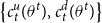 $\big \{ c_{t}^{u}( \theta ^{t}) ,c_{t}^{d}( \theta ^{t}) \big \}$
. This assumption simplifies the analysis while still reflecting the interplay between idiosyncratic shocks and tax evasion in individual decisions and social welfare. Furthermore, it ensures that the solution remains tractable and easy to interpret. Although allowing the saving choice to depend on the auditing status (undetected or detected) could enrich the model, the benefit of added detail may be limited by the complexity it introduces.Footnote
8
Thus we assume that individuals make their saving choices before the outcome of detection is realized.
In every period, individuals are subject to the flow budget constraint, as well as ad hoc borrowing limit:
 \begin{equation} a_{t+1}( \theta ^{t}) \geq \underline {a},\forall \theta ^{t}. \end{equation}
To streamline the exposition of flow budget constraints, let
 $x_{t}( \theta ^{t-1})$
denote the gross income
 $R_{t}a_{t}( \theta ^{t-1}) + ( 1-\tau _{t}) w_{t}n_{t}( \theta ^{t-1})$
. Therefore, budget constraints (2) and (3) reduce to
 \begin{align}& a_{t+1}( \theta ^{t}) +c_{t}^{u}( \theta ^{t}) =x_{t}( \theta ^{t-1}) +\tau _{t}E_{t}( \theta ^{t}) , \end{align}
 \begin{align}&\, a_{t+1}( \theta ^{t}) +c_{t}^{d}( \theta ^{t}) =x_{t}( \theta ^{t-1}) -fE_{t}( \theta ^{t}) . \end{align}
Later, we prove that the tuple of allocations,
 $\big \{ c_{t}^{u}( \theta ^{t}) ,c_{t}^{d}( \theta ^{t}) ,E_{t}( \theta ^{t}) ,a_{t+1}( \theta ^{t}) ,n_{t+1}( \theta ^{t}) \big \}$
, is irrespective of the past history of idiosyncratic shock realizations,
 $\theta ^{t-1}$
. Specifically, these allocations are history-independent but are functions of the current shock realization
 $ \theta _{t}$
. In addition, the gross income,
 $x_{t}( \theta ^{t-1})$
, is solely determined by the aggregate state.Footnote
9
These properties significantly simplify the complexity of a heterogeneous-agent incomplete-markets model with idiosyncratic shocks, thus avoiding the curse of dimensionality.
2.3. Government
The government can issue one-period bonds, levy labor income tax at a rate
 $ \tau _{t}$
, and finance government expenditure
 $G_{t}$
. We assume that each individual is subject to government audits with a probability of
 $p$
. If the evasion is detected, the understated income is penalized at a rate
 $f$
. The government’s flow budget constraint is given by
 \begin{equation} G_{t}+R_{t}B_{t}=\tau _{t}w_{t}N_{t}-Loss_{t}+B_{t+1}, \end{equation}
where
 $Loss_{t}$
denotes the expected net revenue loss due to tax evasion in period
 $t$
, satisfying
 \begin{equation*} Loss_{t}= ( 1-p) \tau _{t}\int E_{t}( \theta ^{t}) d \mathbf{F} ( \theta _{t}) -pf \int E_{t}( \theta ^{t}) d \mathbf{F} ( \theta _{t}) . \end{equation*}
2.4. Market clearing
We assume that government bonds and capital are perfect substitutes for individuals to hedge against idiosyncratic shocks. As such, the asset market clearing requires
 \begin{equation*} K_{t+1}+B_{t+1}=\int a_{t+1}( \theta ^{t}) d\mathbf{F} ( \theta _{t}) . \end{equation*}
The labor market clears according to
 \begin{equation*} N_{t+1}=\int n_{t+1}( \theta ^{t}) d\mathbf{F} ( \theta _{t}) \text{.} \end{equation*}
Goods market clearing condition is given by
 \begin{equation} K_{t+1}+C_{t}+G_{t}=K_{t}^{\alpha }N_{t}^{1-\alpha }+ ( 1-\delta ) K_{t}, \end{equation}
where
 \begin{equation*} C_{t}=\int \big ( ( 1-p) c_{t}^{u}( \theta ^{t}) +pc_{t}^{d}( \theta ^{t}) \big ) d\mathbf{F} ( \theta _{t}) . \end{equation*}
3. Solving household problem
Given prices and taxes
 $\{w_{t},r_{t},\tau _{t}\}$
, a probability of detection
 $p$
, and a penalty rate
 $f$
, individuals choose a sequence of consumption
 $\{c_{t}^{u}(\theta ^{t}),c_{t}^{d}( \theta ^{t}) \},$
labor supply
 $\{n_{t}(\theta ^{t-1})\}$
, and asset holdings
 $ \{a_{t+1}(\theta ^{t})\}$
to maximize the expected lifetime utility as of time zero, subject to flow budget constraints (5) and (6), and the ad hoc borrowing limits (4).
Let
 $\beta ^{t}\lambda _{t}^{u}( \theta ^{t})$
be the multiplier on the flow budget constraint for type
 $\theta ^{t}$
who is undetected,
 $ \beta ^{t}\lambda _{t}^{d}( \theta ^{t})$
the multiplier on the flow budget constraint for type
 $\theta ^{t}$
who gets caught, and
 $\mu _{t}( \theta ^{t})$
the multiplier on the ad hoc borrowing constraints,
 $a_{t+1}( \theta ^{t}) \geq \underline {a},$
 $\forall \theta ^{t}$
.
We derive the FOCs (first-order conditions) with respect to consumption
 $ \big \{ c_{t}^{u}( \theta ^{t}) ,c_{t}^{d}( \theta ^{t}) \big \}$
, labor supply
 $n_{t}( \theta ^{t-1})$
, underreported labor income
 $E_{t}( \theta ^{t})$
, and asset holdings
 $a_{t+1}( \theta ^{t})$
, given
 $x_{t}( \theta ^{t-1})$
:Footnote
10
 \begin{align}( 1-p) \theta _{t}c_{t}^{u}( \theta ^{t}) ^{-\sigma }=\lambda _{t}^{u}( \theta ^{t}) ,\end{align}
 \begin{align} p\theta _{t}c_{t}^{d}( \theta ^{t}) ^{-\sigma }=\lambda _{t}^{d}( \theta ^{t}) , \end{align}
 \begin{align} 1=w_{t} ( 1-\tau _{t}) \int \big ( \lambda _{t}^{u}( \theta ^{t}) +\lambda _{t}^{d}( \theta ^{t}) \big ) d\mathbf{F} ( \theta _{t}) , \end{align}
 \begin{align} \lambda _{t}^{u}( \theta ^{t}) =\frac {f}{\tau _{t}}\lambda _{t}^{d}( \theta ^{t}) , \end{align}
 \begin{align} -\big ( \lambda _{t}^{u}( \theta ^{t}) +\lambda _{t}^{d}( \theta ^{t}) \big ) +\beta R_{t+1}\int \big ( \lambda _{t+1}^{u}( \theta ^{t+1}) +\lambda _{t+1}^{d}( \theta ^{t+1}) \big ) d\mathbf{F}( \theta _{t+1}) +\mu _{t}( \theta ^{t}) =0. \end{align}
The left-hand side (LHS) of (11) represents the marginal utility cost of increasing labor supply by one unit, while the right-hand side (RHS) of (11) represents the marginal utility benefit of doing so. Evidently, a higher tax rate reduces the magnitude of this benefit. From equations (9) and (10), it follows that
 $\lambda _{t}^{u}( \theta ^{t})$
and
 $\lambda _{t}^{d}( \theta ^{t})$
are linked to the marginal utility of consumption in the undetected and detected states, respectively. This relationship highlights how the labor income tax rate distorts the intratemporal margin.
Combining (9) and (10), we derive:
 \begin{eqnarray*} \frac {1-p}{p}\left ( \frac {c_{t}^{u}( \theta ^{t}) }{ c_{t}^{d}( \theta ^{t}) }\right ) ^{-\sigma } &=&\frac {\lambda _{t}^{u}( \theta ^{t}) }{\lambda _{t}^{d}( \theta ^{t}) } \\ &=&\frac {f}{\tau _{t}}, \end{eqnarray*}
where the second equality comes from (12). A higher tax rate
 $\tau _{t}$
increases consumption in the undetected state relative to the detected state. This finding implies that the labor income tax rate can be viewed as a reward in the “gamble” of tax evasion. If individuals evade taxes without being caught, they “win” and enjoy higher consumption compared to those who are “caught” and “lose” the game.
Using (9)–(13), we derive the following proposition to analytically characterize household decisions. Below, we define a cutoff
 $ \theta _{t}^{\ast }$
to distinguish between individuals who are not financially constrained with
 $\theta _{t}\leq \theta _{t}^{\ast }$
and those who are financially constrained with
 $\theta _{t}\gt \theta _{t}^{\ast }$
. This cutoff
 $\theta _{t}^{\ast }$
reflects the severity of the borrowing constraints. When
 $\theta _{t}^{\ast }$
is high, it indicates that a smaller fraction of the population faces binding borrowing constraints. Only individuals exhibiting a strong inclination to consume
 $\theta _{t}$
that surpasses the cutoff
 $\theta _{t}^{\ast }$
are compelled to limit their consumption from increasing as
 $\theta _{t}$
rises.
To simplify notation, we define the consumption weights
 $\kappa _{t}^{u}$
and
 $\kappa _{t}^{d}$
as follows: for undetected households,
 $\kappa _{t}^{u}$
is given by
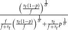 $\frac {\left ( \frac {\tau _{t} ( 1-p) }{f}\right ) ^{ \frac {1}{\sigma }}}{\frac {f}{f+\tau _{t}}\left ( \frac {\tau _{t} ( 1-p) }{f}\right ) ^{\frac {1}{\sigma }}+\frac {\tau _{t}}{f+\tau _{t}}p^{ \frac {1}{\sigma }}}$
, while for detected households,
 $\kappa _{t}^{d}$
is given by
 $\frac {p^{\frac {1}{\sigma }}}{\frac {f}{f+\tau _{t}}\left ( \frac { \tau _{t} ( 1-p) }{f}\right ) ^{\frac {1}{\sigma }}+\frac {\tau _{t}}{ f+\tau _{t}}p^{\frac {1}{\sigma }}}$
. Below, we present the following proposition, which characterizes households’ decision rules by utilizing the borrowing constraint (4), the budget constraints (5)–(6), and the first-order conditions, (9)–(13).
Proposition 1.
Given
 $w_{t},R_{t},R_{t+1}$
and
 $x_{t}=$
 $R_{t}a_{t}\left ( \theta _{t-1}\right ) + ( 1-\tau _{t}) w_{t}n_{t}\left ( \theta _{t-1}\right )$
, household decisions in period
 $t$
on consumption
 $ c_{t}^{u}( \theta ^{t})$
(if undetected) and
 $c_{t}^{d}( \theta ^{t})$
(if detected), labor supply
 $n_{t}( \theta ^{t-1})$
, savings
 $a_{t+1}( \theta ^{t})$
, and underreported income
 $E_{t}( \theta ^{t})$
are given by
 $c_{t}^{u} ( \theta _{t}) =\left ( \frac {\theta _{t}}{\theta _{t}^{\ast }}\right ) ^{\frac {1}{\sigma }} ( x_{t}-\underline {a}) \kappa _{t}^{u}$
, for
 $\theta _{t}\leq \theta _{t}^{\ast },$
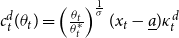 $c_{t}^{d} ( \theta _{t}) =\left ( \frac {\theta _{t}}{\theta _{t}^{\ast }}\right ) ^{\frac {1}{\sigma }} ( x_{t}-\underline {a}) \kappa _{t}^{d}$
, for
 $\theta _{t}\leq \theta _{t}^{\ast },$
 $c_{t}^{u} ( \theta _{t}) = ( x_{t}-\underline {a}) \kappa _{t}^{u}$
, for
 $\theta _{t}\gt \theta _{t}^{\ast },$
 $c_{t}^{d} ( \theta _{t}) = ( x_{t}-\underline {a}) \kappa _{t}^{d}$
, for
 $\theta _{t}\gt \theta _{t}^{\ast },$
 $E_{t} ( \theta _{t}) =\frac {1}{f+\tau _{t}}\left ( \frac {\theta _{t}}{\theta _{t}^{\ast }}\right ) ^{\frac {1}{\sigma }}\left ( x_{t}- \underline {a}\right ) \big( \kappa _{t}^{u}-\kappa _{t}^{d}\big)$
, for
 $ \theta _{t}\leq \theta _{t}^{\ast },$
 $E_{t} ( \theta _{t}) =\frac {1}{f+\tau _{t}}\left ( x_{t}- \underline {a}\right ) \big( \kappa _{t}^{u}-\kappa _{t}^{d}\big)$
, for
 $ \theta _{t}\gt \theta _{t}^{\ast },$
 $a_{t+1} ( \theta _{t}) =x_{t}-\left ( \frac {\theta _{t}}{\theta _{t}^{\ast }}\right ) ^{\frac {1}{\sigma }} ( x_{t}-\underline {a})$
, for
 $\theta _{t}\leq \theta _{t}^{\ast },$
 $a_{t+1} ( \theta _{t}) =\underline {a}$
, for
 $\theta _{t}\gt \theta _{t}^{\ast },$
 $n_{t}\left ( \theta _{t-1}\right ) =\frac {x_{t}-R_{t}a_{t}\left ( \theta _{t-1}\right ) }{ ( 1-\tau _{t}) w_{t}},$
 $x_{t}=\underline {a}+\left ( \frac {\theta _{t}^{\ast }}{\frac {\beta R_{t+1}}{ w_{t+1}\left ( 1-\tau _{t+1}\right ) }\frac {1}{\frac {f}{\tau _{t}}+1}}\right ) ^{\frac {1}{\sigma }}\left [ \frac {\tau _{t}}{f+\tau _{t}}p^{\frac {1}{\sigma } }+\left ( 1-\frac {\tau _{t}}{f+\tau _{t}}\right ) \left ( \frac {\tau _{t} ( 1-p) }{f}\right ) ^{\frac {1}{\sigma }}\right ] ,$
where the cutoff
 $\theta _{t}^{\ast }$
is determined by
 \begin{equation} \frac {w_{t+1}\left ( 1-\tau _{t+1}\right ) }{w_{t} ( 1-\tau _{t}) } =\beta R_{t+1}\left ( \mathbf{F}\big ( \theta _{t}^{\ast }\big) +\int _{\theta \gt \theta _{t}^{\ast }}\frac {\theta }{\theta _{t}^{\ast }}d \mathbf{F}( \theta ) \right ) . \end{equation}
Proof. The proof is relegated to Appendix A.
Proposition1 shows that individuals with a lower inclination to consume, as indicated by
 $\theta _{t}$
below the cutoff
 $\theta _{t}^{\ast }$
, are not financially constrained. These individuals follow the consumption rule
 $\left ( \frac {\theta _{t}}{\theta _{t}^{\ast }}\right ) ^{\frac {1}{\sigma }} ( x_{t}-\underline {a}) \kappa _{t}^{i}$
,
 $ i= \{ u,d\}$
, where the consumption share
 $\kappa _{t}^{i}$
denotes the consumption share, depending on whether the individual is undetected (
 $u$
) or detected (
 $d$
) in tax evasion. Their tax evasion decision follows
 $\frac {1}{f+\tau _{t}}\left ( \frac {\theta _{t}}{\theta _{t}^{\ast }}\right ) ^{\frac {1}{\sigma }} ( x_{t}-\underline {a}) \big( \kappa _{t}^{u}-\kappa _{t}^{d}\big)$
, where the ratio
 $\left ( \frac {\theta _{t}}{\theta _{t}^{\ast }}\right ) ^{\frac {1}{\sigma }}$
captures their relative desire to consume. Among these unconstrained individuals, those with larger
 $\theta _{t}$
(but still less than
 $\theta _{t}^{\ast }$
) tend to evade more taxes in pursuit of greater consumption if undetected. By contrast, individuals with
 $\theta _{t}\gt$
 $\theta _{t}^{\ast }$
, who have a stronger preference for consumption, are financially constrained. The borrowing limit prevents them from fully satisfying their consumption desires, leading to an alternative consumption rule:
 $ ( x_{t}-\underline {a}) \kappa _{t}^{i}$
,
 $i= \{ u,d\}$
. Their tax evasion behavior similarly adjusts to
 $\frac {1}{f+\tau _{t}}\left ( x_{t}- \underline {a}\right ) \big( \kappa _{t}^{u}-\kappa _{t}^{d}\big)$
. Notably, both their consumption and tax evasion decisions no longer depend on the ratio
 $\left ( \frac {\theta _{t}}{\theta _{t}^{\ast }}\right ) ^{\frac {1}{\sigma }}$
, underscoring the influence of the binding borrowing constraint. We elaborate further on these decision rules in the discussion below.
According to the expressions of
 $\big \{ c_{t}^{u} ( \theta _{t}) ,c_{t}^{d} ( \theta _{t}) \big \} _{t=0}^{\infty }$
, when the inclination to consume is low,
 $\theta _{t}\leq \theta _{t}^{\ast }$
, consumption
 $c_{t}^{u}$
and
 $c_{t}^{d}$
depend on the fraction
 $\left ( \frac { \theta _{t}}{\theta _{t}^{\ast }}\right ) ^{\frac {1}{\sigma }}$
of the income
 $x_{t}-\underline {a}$
, weighted by
 $\kappa _{t}^{u}$
for
 $c_{t}^{u}$
and
 $ \kappa _{t}^{d}$
for
 $c_{t}^{d}$
, respectively. It follows that the ratio
 $ \frac {c_{t}^{u}}{c_{t}^{d}}$
can be expressed as
 $\left ( \frac {fp}{\tau _{t} ( 1-p) }\right ) ^{\frac {1}{\sigma }}$
. As
 $p$
or
 $f$
decreases or
 $\tau _{t}$
increases, the undetected consumption
 $c_{t}^{u}$
becomes relatively higher than the detected consumption
 $c_{t}^{d}$
. For those with low urge to consume, their consumption increases in
 $\theta _{t}$
. On the contrary, for individuals with a strong inclination to consume,
 $ \theta _{t}\gt \theta _{t}^{\ast }$
, the borrowing constraint limits them to consume as
 $\theta _{t}$
increases. It can be seen from the expressions of
 $c_{t}^{u} ( \theta _{t})$
and
 $c_{t}^{d} ( \theta _{t})$
with
 $\theta _{t}\gt \theta _{t}^{\ast }$
in Proposition1 that both
 $c_{t}^{u}$
and
 $c_{t}^{d}$
solely depend on the income
 $x_{t}-\underline {a}$
, weighted by
 $\kappa _{t}^{u}$
for
 $c_{t}^{u}$
and
 $\kappa _{t}^{d}$
for
 $c_{t}^{d}$
, respectively.
As captured by the expression of
 $E_{t} ( \theta _{t})$
with
 $ \theta _{t}\leq \theta _{t}^{\ast }$
in Proposition1, the extent of underreported labor income is proportional to the preference shock
 $\theta _{t}^{\frac {1}{\sigma }}$
. The stronger the inclination for consumption, the greater the understatement of labor income. We assume
 $ \frac {\tau _{t} ( 1-p) }{f}\gt p$
, or equivalently
 $\kappa _{t}^{u}\gt \kappa _{t}^{d}$
, so as to guarantee
 $E_{t}( \theta ^{t}) \gt 0$
.
Let us examine the case where
 $\underline {a}=0$
. It immediately follows that
 \begin{align}& \frac {E_{t} ( \theta _{t}) }{x_{t}}=\left ( \frac {\theta _{t}}{ \theta _{t}^{\ast }}\right ) ^{\frac {1}{\sigma }}\frac {\kappa _{t}^{u}-\kappa _{t}^{d}}{f+\tau _{t}}\text{, for }\theta _{t}\leq \theta _{t}^{\ast }, \end{align}
 \begin{align}&\qquad \frac {E_{t} ( \theta _{t}) }{x_{t}}=\frac {\kappa _{t}^{u}-\kappa _{t}^{d}}{f+\tau _{t}}\text{, for }\theta _{t}\gt \theta _{t}^{\ast }. \end{align}
According to (15) and (16), individuals facing financial constraints, characterized by
 $\theta _{t}\gt \theta _{t}^{\ast }$
, tend to engage in greater tax evasion compared to individuals with
 $\theta _{t}\leq \theta _{t}^{\ast }$
. Essentially, tax evasion acts as a strategy employed by financially constrained individuals to alleviate the adverse impact of financial market imperfections on their situations. This is achieved despite the uncertainty associated with tax evasion, which functions as a gamble.
Furthermore, when considering
 $\sigma =1$
, the ratio in (15) and (16), namely
 $\frac {\kappa _{t}^{u}-\kappa _{t}^{d}}{f+\tau _{t}}$
, simplifies to
 $\frac { ( 1-p) \tau _{t}-fp}{f}$
. It is evident that given by the cutoff
 $\theta _{t}^{\ast }$
, the extent of tax evasion relative to gross income rises in
 $\tau _{t}$
for all individuals.
In light of the expression of
 $\left \{ E_{t} ( \theta _{t}) \right \} _{t=0}^{\infty }$
, the resource devoted to tax evasion can be expressed by
 \begin{align} \left ( f+\tau _{t}\right ) \int E_{t}( \theta )\; d\mathbf{F}( \theta ) &=\int _{\theta \leq \theta _{t}^{\ast }}\left ( \frac {\theta }{\theta _{t}^{\ast }}\right ) ^{\frac {1}{\sigma }}\left ( x_{t}-\underline {a} \right ) \big( \kappa _{t}^{u}-\kappa _{t}^{d}\big) d\mathbf{F}( \theta ) \notag \\ &\quad +\int _{\theta \gt \theta _{t}^{\ast }} ( x_{t}-\underline {a}) \big( \kappa _{t}^{u}-\kappa _{t}^{d}\big) d\mathbf{F}( \theta ) \notag \\ &= ( x_{t}-\underline {a}) \big( \kappa _{t}^{u}-\kappa _{t}^{d}\big) \left [ \begin{array}{c} \int _{\theta \leq \theta _{t}^{\ast }}\left ( \frac {\theta }{\theta _{t}^{\ast }}\right ) ^{\frac {1}{\sigma }}d\mathbf{F}( \theta ) \\ +\left ( 1-\mathbf{F}\big ( \theta _{t}^{\ast }\big) \right ) \end{array} \right ] . \end{align}
On the basis of (17), we can further characterize the expected net revenue loss due to tax evasion,
 $Loss_{t}$
, given by
 \begin{align} Loss_{t} &= ( 1-p) \tau _{t}\int E_{t}( \theta )\; d\mathbf{F}( \theta ) -pf\int E_{t}( \theta )\; d\mathbf{F }( \theta ) \notag \\ &=\left ( \frac {\tau _{t}}{f+\tau _{t}}-p\right ) \big( \kappa _{t}^{u}-\kappa _{t}^{d}\big) ( x_{t}-\underline {a}) \left [ \int _{\theta \leq \theta _{t}^{\ast }}\left ( \frac {\theta }{\theta _{t}^{\ast }}\right ) ^{\frac {1}{\sigma }}d\mathbf{F}( \theta ) +1- \mathbf{F}\big ( \theta _{t}^{\ast }\big) \right ] . \end{align}
In light of Proposition1, we know individuals with
 $\theta _{t}\gt \theta _{t}^{\ast }$
hold
 $a_{t+1} ( \theta _{t}) =\underline { a}$
, indicating that those with a strong preference for immediate consumption are constrained from borrowing, forcing them to maintain asset holdings at the lower bound
 $\underline {a}$
. For those with less inclination toward consumption who thus do not hit borrowing constraints,
 $a_{t+1} ( \theta _{t})$
can be rewritten as
 \begin{equation*} a_{t+1} ( \theta _{t}) =x_{t}\left ( 1-\left ( \frac {\theta _{t}}{ \theta _{t}^{\ast }}\right ) ^{\frac {1}{\sigma }}\right ) +\left ( \frac {\theta _{t}}{\theta _{t}^{\ast }}\right ) ^{\frac {1}{\sigma }}\underline {a}, \end{equation*}
implying that their asset holding is negatively correlated with
 $\theta _{t}$
, given that
 $x_{t}\gt \underline {a}$
.
Thus, individuals with less propensity toward consumption do not need to borrow and are able to accumulate more assets. In contrast, individuals with a strong urge to consume tend to seek more borrowing so as to meet their consumption needs. However, borrowing constraints prevent them from borrowing freely, forcing their asset holdings to remain at or above
 $ \underline {a}$
. The results regarding
 $a_{t+1} ( \theta _{t})$
, as presented in Proposition1, mirror findings derived from a traditional Aiyagari economy with productivity shocks, where individuals with lower productivity levels tend to borrow more to smooth consumption. Yet, binding borrowing constraints limit their borrowing, leaving them with asset holdings at the minimum level
 $\underline {a}$
.
The characteristic feature of capital per capita over-accumulation in Aiyagari economy is also preserved in (14). Equation (14) corresponds to the aggregate Euler equation. The marginal utility cost of saving one unit of the commodity is
 $\int \big ( \lambda _{t}^{u}( \theta ^{t}) +\lambda _{t}^{d}( \theta ^{t}) \big ) d\mathbf{F} ( \theta _{t})$
, which is the reciprocal of after-tax wage rate at time
 $t$
, according to (11). Note that both
 $\lambda _{t}^{u}$
and
 $\lambda _{t}^{d}$
represent the period-
 $t$
marginal utility in undetected and detected states, respectively. The marginal utility benefit from such saving is characterized by
 $\frac {\beta R_{t+1}}{w_{t+1}\left ( 1-\tau _{t+1}\right ) }$
, multiplied by
 $\mathbf{F}\big ( \theta _{t}^{\ast }\big) +\int _{\theta \gt \theta _{t}^{\ast }}\frac {\theta }{\theta _{t}^{\ast }}d\mathbf{F}( \theta )$
. The reciprocal of
 $w_{t+1}\left ( 1-\tau _{t+1}\right )$
again denotes the expected period-
 $t+1$
marginal utility. Alternatively, the aggregate Euler equation can be interpreted in this manner. The LHS of (14) represents the marginal cost of saving an additional unit, while the RHS captures the marginal benefit of doing so. If the after-tax wage in period
 $t+1$
exceeds that in period
 $t$
, individuals are inclined to front-load consumption because saving, relative to labor supply in period
 $t+1$
, becomes less appealing from the perspective of period
 $t$
. This interpretation highlights the role of the ratio
 $\frac { w_{t+1}\left ( 1-\tau _{t+1}\right ) }{w_{t} ( 1-\tau _{t}) }$
in shaping decisions along the intertemporal margin.
In a representative-agent model, the Euler equation is expressed as
 $\frac {1 }{w_{t} ( 1-\tau _{t}) }=\frac {\beta R_{t+1}}{w_{t+1}\left ( 1-\tau _{t+1}\right ) }$
. In contrast, in a heterogeneous-agent model, an additional term emerges in the aggregate Euler equation, characterizing the impact of binding borrowing constraints on the moments of the preference distribution
 $ \mathbf{F}\big ( \theta _{t}^{\ast }\big) +\int _{\theta \gt \theta _{t}^{\ast }}\frac {\theta }{\theta _{t}^{\ast }}d\mathbf{F}( \theta )$
. Specifically, if no one hits the borrowing constraint, i.e.,
 $\left \{ \left . \theta \right \vert \theta \gt \theta _{t}^{\ast }\right \} =\varnothing$
, this term
 $\mathbf{F}\big ( \theta _{t}^{\ast }\big) +\int _{\theta \gt \theta _{t}^{\ast }}\frac {\theta }{\theta _{t}^{\ast }}d\mathbf{F}( \theta )$
will reduce to 1. Whereas, when a non-measure-zero fraction of the population faces binding borrowing constraints, the term
 $\mathbf{F}\big ( \theta _{t}^{\ast }\big) +\int _{\theta \gt \theta _{t}^{\ast }}\frac {\theta }{ \theta _{t}^{\ast }}d\mathbf{F}( \theta )$
is greater than 1, leading to
 $\frac {1}{w_{t} ( 1-\tau _{t}) }\gt \frac {\beta R_{t+1}}{ w_{t+1}\left ( 1-\tau _{t+1}\right ) }$
. As a result, the steady-state
 $\beta R$
is less than 1, reflecting the well-known outcome of an Aiyagari-style economy.
As shown in (14), the cutoff
 $\theta _{t}^{\ast }$
is determined by
 $ \frac {w_{t+1}\left ( 1-\tau _{t+1}\right ) }{w_{t} ( 1-\tau _{t}) }$
,
 $\beta R_{t+1}$
, and the distribution of
 $\mathbf{F}$
. Moreover, Proposition1 indicates that for
 $\theta _{t}\leq \theta _{t}^{\ast }$
,
 $c_{t}^{u} ( \theta _{t}) ,c_{t}^{d} ( \theta _{t})$
,
 $a_{t+1} ( \theta _{t})$
, and
 $E_{t} ( \theta _{t})$
are contingent on the current shock realization relative to the cutoff
 $\frac {\theta _{t}}{\theta _{t}^{\ast }}$
and the aggregate state at time
 $t$
. This aggregate state is determined by factor prices
 $\left \{ w_{t},w_{t+1},R_{t+1}\right \}$
, along with the policy instruments
 $\left \{ \tau _{t},\tau _{t+1},f,p\right \}$
, the lower bound on the asset holding
 $ \underline {a}$
, and the parameters
 $\sigma$
and
 $\beta$
. Notably, the expression for
 $x_{t}$
, as seen in Proposition1, implies that the equilibrium
 $x_{t}$
depends on the aggregate state. All the derivations in Proposition1 are based on the assumptions that an i.i.d. preference shock, a flat tax rate, and the labor decision being made prior to the shock realization. In particular, these assumptions ensure the independence of the history of shock realizations. As noted by Chien and Wen (Reference Chien and Wen2022), a “target” income level
 $x_{t}$
can be determined, since labor supply is chosen flexibly to meet
 $x_{t},$
given asset holdings
 $a_{t}( \theta ^{t-1})$
. This flexibility in labor supply adjustment is a direct consequence of these assumptions. As
 $ x_{t}$
depends solely on the aggregate state and is identical across all individuals, differences in households’ decisions regarding consumption, tax evasion, and savings arise only from variations in their current preference shock realizations.
For
 $\theta _{t}\gt \theta _{t}^{\ast }$
,
 $c_{t}^{u} ( \theta _{t}) ,c_{t}^{d} ( \theta _{t})$
, and
 $E_{t} ( \theta _{t})$
are reliant solely on the aggregate state. To understand the factors underpinning the aggregate state, we must solve for the cutoff and factor prices, which are endogenous and market-determined. Note that the cutoff
 $ \theta _{t}^{\ast }$
which identifies the minimum level of the preference shock above which individuals (i.e., those with
 $\theta _{t}\gt \theta _{t}^{\ast }$
) face a binding borrowing constraint. As such, the cutoff also determines the proportion of financially constrained individuals and serves as a measure of the severity of financial market frictions.
Given that Proposition1 paves the way for characterizing solutions to the household problem, the next step is to establish a competitive equilibrium, which is essential for deriving
 $\theta _{t}^{\ast }$
and factor prices.
3.1. Competitive equilibrium
A competitive equilibrium of the model economy is defined in the standard way.
Definition 1.
Given the initial capital
 $K_{0}$
and initial bond level
 $B_{0}$
, a competitive equilibrium is defined as sequences of prices
 $ \{w_{t},r_{t},\tau _{t},B_{t}\}_{t=0}^{\infty }$
, a probability of detection
 $p$
, a penalty rate
 $f$
, aggregate allocations
 $\{C_{t},N_{t},K_{t+1} \}_{t=0}^{\infty }$
, and individual allocations
 $\{c_{t}^{u}(\theta ^{t}),c_{t}^{d}(\theta ^{t}),n_{t}(\theta ^{t-1}), a_{t+1}( \theta ^{t}) ,E_{t}( \theta ^{t}) \}_{t=0}^{\infty }$
, such that
-
1. Given
 $\{w_{t},r_{t},\tau _{t},B_{t},p,f\}_{t=0}^{\infty }$
, the sequences
$\{c_{t}^{u}(\theta ^{t}),c_{t}^{d}(\theta ^{t}),n_{t}(\theta ^{t-1}),a_{t+1}( \theta ^{t}) ,E_{t}( \theta ^{t}) \}_{t=0}^{\infty }$
solve the household problem.
-
2. Given
$\{w_{t},r_{t}\}_{t=0}^{\infty }$
, the sequences
$ \{K_{t},N_{t}\}_{t=0}^{\infty }$
solve the representative firm’s problem.
-
3. The no-arbitrage condition holds:
$R_{t}=1+r_{t}$
for all
$t\geq 0$
. -
4. The government’s flow budget constraint holds in every period.
-
5. All markets clear for all
$t\geq 0$
.




By consolidating each type’s flow budget constraint with government budget constraints, firms’ optimal conditions, and market clearing conditions, we can obtain the exact resource constraint expressed in (8). Note that according to Lemma1, the gross income
 $x_{t}( \theta ^{t-1})$
is history-independent of
 $\theta ^{t-1}$
. Integrating over (5) and (6) with the corresponding probability over
 $\theta _{t}$
, we obtain
 \begin{equation} K_{t+1}+B_{t+1}+C_{t}=x_{t}+Loss_{t}, \end{equation}
where we integrate over
 $c_{t}^{u} ( \theta _{t})$
and
 $ c_{t}^{d} ( \theta _{t})$
with respect to
 $\theta _{t}$
and utilize
 $K_{t+1}+B_{t+1}=\int a_{t+1}( \theta )\; d\mathbf{F}( \theta )$
and (18). From the definition of
 $x_{t}$
, we have
 \begin{equation} x_{t}=R_{t}K_{t}+ ( 1-\tau _{t}) w_{t}N_{t}. \end{equation}
By firms’ first-order conditions, (20) can be written as
 \begin{eqnarray} x_{t} &=&\left ( 1+F_{K}(K_{t},N_{t})-\delta \right ) \left ( K_{t}+B_{t}\right ) + ( 1-\tau _{t}) F_{N}(K_{t},N_{t})N_{t} \notag \\ &=&K_{t}^{\alpha }N_{t}^{1-\alpha }+ ( 1-\delta ) K_{t}+R_{t}B_{t}-\tau _{t}w_{t}N_{t} \notag \\ &=&K_{t}^{\alpha }N_{t}^{1-\alpha }+ ( 1-\delta ) K_{t}-Loss_{t}+B_{t+1}-G_{t}, \end{eqnarray}
where the second line comes from the Euler theorem and the last line is due to (7).
Inserting (21) into (19) immediately gives (8).
Finally, by using expressions of
 $\big \{ c_{t}^{u} ( \theta _{t}) ,c_{t}^{d} ( \theta _{t}) \big \} _{t=0}^{\infty }$
we characterize aggregate consumption, given by
 \begin{eqnarray} C_{t} &=&\int _{\theta \leq \theta _{t}^{\ast }}\big ( pc_{t}^{d}( \theta ) + ( 1-p) c_{t}^{u}( \theta ) \big ) d \mathbf{F}( \theta ) +\int _{\theta \gt \theta _{t}^{\ast }}\big ( pc_{t}^{d}( \theta ) + ( 1-p) c_{t}^{u}( \theta ) \big ) d\mathbf{F}( \theta ) \notag \\ &=& ( x_{t}-\underline {a}) \big [ ( 1-p) \kappa _{t}^{u}+p\kappa _{t}^{d}\big ] \left [ \int _{\theta \leq \theta _{t}^{\ast }}\left ( \frac {\theta }{\theta _{t}^{\ast }}\right ) ^{\frac {1}{\sigma }}d \mathbf{F}( \theta ) +1-\mathbf{F}\big ( \theta _{t}^{\ast }\big) \right ] . \end{eqnarray}
Turning to aggregate capital, we employ the expression of
 $\left \{ a_{t+1} ( \theta _{t}) \right \} _{t=0}^{\infty }$
to yield
 \begin{align} K_{t+1}&=\int a_{t+1}( \theta )\; d\mathbf{F}( \theta ) -B_{t+1}\notag \\ &=x_{t}\mathbf{F}\big ( \theta _{t}^{\ast }\big) -\left ( x_{t}- \underline {a}\right ) \int _{\theta \leq \theta _{t}^{\ast }}\left ( \frac { \theta }{\theta _{t}^{\ast }}\right ) ^{\frac {1}{\sigma }}d\mathbf{F}( \theta ) +\underline {a}\left ( 1-\mathbf{F}\big ( \theta _{t}^{\ast }\big) \right ) -B_{t+1}, \end{align}
where the second equality comes from the asset-market clearing condition.
Note that the cash on hand
 $x_{t}$
, as shown in (21), is independent of the idiosyncratic shock
 $\theta _{t}$
and thus remains the same across households. As such, as indicated by Proposition1, there is no redistributive effect on consumption, asset holdings, or tax evasion.
Despite not addressing the wealth inequality caused by tax evasion,Footnote 11 our contribution is to analytically emphasize its impact, along with related policies, on aggregate allocative efficiency. By eliminating the wealth-redistribution effect, we focus on how tax evasion influences individuals’ self-insurance and aggregate allocative efficiency within the HAIM model. As such, this framework may facilitate the accentuation of the role of tax evasion solely on the efficiency side.
4. Steady state
This section characterizes the steady state. We use the subscript
 $ss$
to denote the period in which the economy sits in a steady state. We analytically derive expressions for steady-state allocations, including
 $ \theta _{ss}^{\ast }$
,
 $K_{ss}$
,
 $N_{ss}$
,
 $C_{ss}$
,
 $\ x_{ss}$
, and
 $\int E_{ss}( \theta )\; d\mathbf{F}( \theta )$
, laying the groundwork for the numerical analysis in the following section. Furthermore, the analytical solution enables us to isolate and examine the effects of policy instruments on key variables. We begin by characterizing the steady state cutoff
 $\theta _{ss}^{\ast }$
, and then examine how these policy instruments may mitigate or exacerbate the adverse effects of financial market frictions on allocations.
In order to investigate the impact of fiscal instruments on the cutoff
 $ \theta _{ss}^{\ast }$
, we undertake a simple analysis by setting
 $\underline { a}=0$
,
 $B_{ss}=0$
,
 $G_{ss}=gF\left ( K_{ss},N_{ss}\right )$
with
 $g\lt 1$
, and
 $ \tau _{t}=\tau _{ss}$
, for
 $t\geq ss$
.
In addition, we also impose
Assumption 1. The production function is given by
 \begin{equation*} Y=F( K,N) =K^{\alpha }N^{1-\alpha }\text{, with }0\lt \alpha \lt 1\text{ .} \end{equation*}
Given Assumption1, we derive
 $R_{t}=1+\alpha \left ( \frac {K_{t}}{N_{t}}\right ) ^{\alpha -1}-\delta$
and
 $w_{t}=\left ( 1-\alpha \right ) \left ( \frac {K_{t}}{N_{t}}\right ) ^{\alpha }\ \ $
for all
 $ t\geq 0$
.
4.1. Characterizing the steady state
Equipped with the assumptions above, the properties of the competitive equilibrium and Proposition1, we are ready to solve for the steady-state cutoff
 $\theta _{ss}^{\ast }$
,
 $\ x_{ss}$
, and
 $\int E_{ss}( \theta )\; d\mathbf{F}( \theta )$
.
Given
 $\underline {a}=0$
, we write the steady-state version of (14) as
 \begin{equation} \frac {1}{\beta R_{ss}}=\mathbf{F}\big ( \theta _{ss}^{\ast }\big ) +\frac {1 }{\theta _{ss}^{\ast }}\int _{\theta \gt \theta _{ss}^{\ast }}\theta d\mathbf{F} ( \theta ) , \end{equation}
which implies that the cutoff
 $\theta _{ss}^{\ast }$
is determined by
 $ R_{ss}$
. To explicitly express
 $\theta _{ss}^{\ast }$
, we must determine
 $ R_{ss}$
. To achieve this, we solve for aggregate allocations, since
 $ R_{ss}=1+\alpha \left ( \frac {K_{ss}}{N_{ss}}\right ) ^{\alpha -1}-\delta$
.
To align our finding with the classic result in the Aiyagari model
 $\beta R_{ss}\lt 1$
, we delve further into the market Euler equation (24) more. Note that (24) indicates that once
 $1-\mathbf{F}\big( \theta _{ss}^{\ast }\big) \gt 0$
, it must be the case that
 $\mathbf{F}\big( \theta _{ss}^{\ast }\big) +\int _{\theta \gt \theta _{ss}^{\ast }}\frac {\theta }{ \theta _{ss}^{\ast }}d\mathbf{F}( \theta )$
exceeds 1. As such, the economy features
 $\beta R_{ss}\lt 1$
at steady state, consistent with the well-known result from the Aiyagari model. To uphold the result
 $\beta R_{ss}\lt 1$
, individuals with non-zero measure face constrained consumption in that they encounter positive preference shocks that urge them to consume more. However, financial market frictions prevent them from borrowing to fulfill this demand. In a typical Aiyagari economy with productivity shocks, a similar rationale applies, with the modification that individuals facing adverse productivity shocks often wish to borrow more to smooth consumption. Financial frictions, however, inhibit such borrowing.
To facilitate the analysis, we impose the assumption on the cumulative distribution function
 $\mathbf{F}$
:
Assumption 2.
The random variable
 $\theta$
follows a Pareto distribution with a shape parameter
 $v\gt 1$
, expressed as
 $\mathbf{F}( \theta ) =1-\left ( \frac {\theta _{L}}{\theta }\right ) ^{v}$
.
Under Assumption2, we derive
 $\int _{\theta \leq \theta _{ss}^{\ast }}\left ( \frac {\theta }{\theta _{ss}^{\ast }}\right ) ^{\frac {1}{ \sigma }}d\mathbf{F}( \theta ) =\frac {v\sigma }{1-v\sigma }\left [ \left ( \frac {\theta _{L}}{\theta _{ss}^{\ast }}\right ) ^{v}-\left ( \frac { \theta _{L}}{\theta _{ss}^{\ast }}\right ) ^{\frac {1}{\sigma }}\right ]$
and
 $ \int _{\theta \gt \theta _{ss}^{\ast }}\theta d\mathbf{F}( \theta ) = \frac {v\left ( \theta _{L}\right ) ^{v}}{v-1}\big( \theta _{ss}^{\ast }\big) ^{1-v}$
. As a result, the steady-state version of Euler equation (24) can be written as
 \begin{equation*} \frac {1}{\beta R_{ss}}=1+\frac {1}{v-1}\left ( \frac {\theta _{L}}{\theta _{ss}^{\ast }}\right ) ^{v}, \end{equation*}
implying that the term
 $\frac {1}{v-1}\left ( \frac {\theta _{L}}{\theta _{ss}^{\ast }}\right ) ^{v}$
, which is strictly positive provided that
 $ \theta _{ss}^{\ast }\lt \infty$
, drives down
 $\beta R_{ss}$
from 1. In addition, as more individuals face binding borrowing limits, the cutoff
 $ \theta _{ss}^{\ast }$
decreases, which is accompanied by a reduction of
 $ \beta R_{ss}$
. It reflects the well-known feature of an Aiyagari-type economy at steady state; that is, individuals’ precautionary savings motive brings about capital overaccumulation.
The following proposition characterizes how the steady-state cutoff
 $\theta _{ss}^{\ast }$
is determined.
Proposition 2.
Impose Assumptions 1–2,
 $\underline {a}=0$
,
 $B_{ss}=0$
, and
 $G_{ss}=gF\left ( K_{ss},N_{ss}\right )$
with
 $g\lt 1$
. At the steady state, the cutoff
 $\theta _{ss}^{\ast }$
satisfies
 \begin{equation} \frac {1}{v-1}\left ( \frac {\theta _{L}}{\theta _{ss}^{\ast }}\right ) ^{v}= \frac {1}{\beta }\left [ 1+\frac {\alpha +g-1}{1-g}\delta +\frac {\alpha \Phi }{ 1-g}\frac {\Gamma \big( \theta _{ss}^{\ast }\big) }{1-\Gamma \big( \theta _{ss}^{\ast }\big) }\right ] ^{-1}-1, \end{equation}
where
 \begin{eqnarray} \Gamma \big( \theta _{ss}^{\ast }\big) &\equiv &\int _{\theta \leq \theta _{ss}^{\ast }}\left ( \frac {\theta }{\theta _{ss}^{\ast }}\right ) ^{\frac {1}{ \sigma }}d\mathbf{F}( \theta ) +1-\mathbf{F}\big( \theta _{ss}^{\ast }\big) \notag \\ &=&\frac {1}{1-v\sigma }\left ( \frac {\theta _{L}}{\theta _{ss}^{\ast }} \right ) ^{v}-\frac {v\sigma }{1-v\sigma }\left ( \frac {\theta _{L}}{\theta _{ss}^{\ast }}\right ) ^{\frac {1}{\sigma }}, \end{eqnarray}
and
 \begin{equation} \Phi \equiv ( 1-p) \kappa _{ss}^{u}+p\kappa _{ss}^{d}. \end{equation}
In addition, when
 $\sigma \geq 1$
and the condition
 $\frac {1}{\beta }\frac { 1-g}{\left ( 1-g\right ) ( 1-\delta ) +\alpha \left ( \delta +\Phi \right ) }-1\lt \frac {1}{v-1}$
holds, the cutoff
 $\theta _{ss}^{\ast }$
is uniquely determined.
Proof. The proof is relegated to Appendix B.
Proposition2 suggests that given
 $\sigma \geq 1$
, a condition supported by empirical evidence, and the condition
 $\frac {1}{ \beta }\frac {1-g}{\left ( 1-g\right ) ( 1-\delta ) +\alpha \left ( \delta +\Phi \right ) }-1\lt \frac {1}{v-1}$
, a unique cutoff
 $\theta _{ss}^{\ast }$
can be identified. As we demonstrate later, this proposition allows us to examine how the cutoff
 $\theta _{ss}^{\ast }$
adjusts in response to the changes in policy instruments.
Because of the complexity of
 $\Phi$
, in the following analysis we focus on the case of
 $\sigma =1$
. We define
 $\bar {\Phi }=\left . \Phi \right \vert _{\sigma =1}=\frac {f+\tau _{ss}}{\tau _{ss}}p^{2}+\frac {f+\tau _{ss}}{f} ( 1-p) ^{2}$
and
 $\bar {\Gamma }\big( \theta _{ss}^{\ast }\big) =\left . \Gamma \big( \theta _{ss}^{\ast }\big) \right \vert _{\sigma =1 \text{ }}=\frac {1}{1-v}\left ( \frac {\theta _{L}}{\theta _{ss}^{\ast }} \right ) ^{v}-\frac {v}{1-v}\left ( \frac {\theta _{L}}{\theta _{ss}^{\ast }} \right )$
.
4.2. Cutoff
$ \theta _{ss}^{\ast }$
and tax evasion at steady state

Below we explore how the steady state cutoff
 $\theta _{ss}^{\ast }$
responds to the changes in
 $p$
,
 $f$
, and
 $\tau _{ss}$
, in the presence of tax evasion. Notably, the cutoff size inversely reflects the intensity of financial market frictions.Footnote
12
We present the following proposition and discuss the intuition thereafter.
Proposition 3.
Impose Assumptions
1
and
2
,
 $\sigma =1$
,
 $\underline {a}=0$
,
 $B_{ss}=0$
, and
 $ G_{ss}=gF\left ( K_{ss},N_{ss}\right )$
with
 $g\lt 1$
. Under the condition
 $ \frac { ( 1-p) \tau _{ss}}{f}\gt p$
, the steady-state cutoff,
 $\theta _{ss}^{\ast }$
, increases in
-
1. a lower probability of auditing
$p$
, -
2. a smaller
$f$
, and
-
3. a higher
$\tau _{ss}$
.


Proof. The proof is relegated to Appendix C.
The first result in Proposition3,
 $\frac {\partial \theta _{ss}^{\ast }}{\partial p}\lt 0$
, implies that holding other factors constant, a higher probability of auditing increases the proportion of financially constrained individuals. Intuitively, a reduced probability of auditing provides individuals with an incentive to engage in tax evasion. While individuals who undergo audits face a higher likelihood of encountering borrowing constraints due to increased penalties,
 $\left ( f+\tau \right ) E$
, paid, reduced tax compliance mitigates the impact of financial market imperfections on consumption, labor supply, and savings for other individuals. A decline in
 $p$
, ceteris paribus, leads to a decrease in in the proportion of the population trapped in financial difficulties.
Next, based on the second result in Proposition3, which shows
 $ \frac {\partial \theta _{ss}^{\ast }}{\partial f}\lt 0$
, we find that a less severe punishment enhances financial efficiency. The intuition is as follows. Provided that
 $\sigma =1$
and
 $\underline {a}=0$
, (17) simplifies to
 $\int E_{ss}( \theta )\; d\mathbf{F}( \theta ) =\frac {\tau _{ss} ( 1-p) -fp}{f}\frac {x_{ss}}{\tau _{ss}} \left [ \int _{\theta \leq \theta _{ss}^{\ast }}\frac {\theta }{\theta _{ss}^{\ast }}d\mathbf{F}( \theta ) +\left ( 1-\mathbf{F}\big( \theta _{ss}^{\ast }\big) \right ) \right ]$
. This expression indicates that, holding
 $x_{ss}$
and
 $\theta _{ss}^{\ast \text{ }}$
unchanged, a reduction in the penalty rate directly boosts the extent of tax evasion.Footnote
13
Since tax evasion, in aggregate, acts as a buffer against the negative impact of financial market frictions, it reduces the proportion of the population facing constrained consumption.
Finally, we turn to the third result in Proposition3, which reveals
 $\frac {\partial \theta _{ss}^{\ast }}{\partial \tau _{ss}}\gt 0$
. To understand the rationale, we again utilize the expression
 $\int E_{ss}( \theta )\; d\mathbf{F}( \theta ) =\frac { ( 1-p) \tau _{ss}-fp}{f}\frac {x_{ss}}{\tau _{ss}}\left [ \int _{\theta \leq \theta _{ss}^{\ast }}\frac {\theta }{\theta _{ss}^{\ast }}d\mathbf{F}( \theta ) +1-\mathbf{F}\big( \theta _{ss}^{\ast }\big) \right ]$
. It can be seen that with
 $x_{ss}$
and
 $\theta _{ss}^{\ast \text{ }}$
held fixed, an increase in
 $\tau _{ss}$
directly encourages households to engage in more tax evasion. This aligns with the intuition that a higher level of tax evasion can help mitigate the adverse effects of financial market frictions on consumption.
Recall that
 $\forall \theta$
,
 $E_{ss}( \theta ) \gt 0$
if
 $\frac { ( 1-p) \tau _{ss}}{f}\gt p$
, and
 $E_{ss}( \theta ) =0$
if
 $\frac { ( 1-p) \tau _{ss}}{f}=p$
, as shown in Proposition1. In light of Proposition3, as the condition
 $\frac { ( 1-p) \tau _{ss}}{f}\gt p$
holds, which guarantees that
 $ E_{ss}( \theta ) \gt 0$
, a positive effect of
 $\tau _{ss}$
on
 $ \theta _{ss}^{\ast }$
arises. Based on the rationale above, we know that mechanism through which raising
 $\tau _{ss}$
impacts the cutoff
 $\theta _{ss}^{\ast }$
is built on the existence of
 $E_{ss}( \theta ) \gt 0$
. Put differently, positive tax evasion facilitates the upward pressure of
 $ \tau _{ss}$
on the cutoff
 $\theta _{ss}^{\ast }$
. This can also be interpreted as follows: tax evasion helps alleviate the adverse effect of idiosyncratic shocks in the face of a higher tax rate. Moreover, the upward pressure on both
 $\theta _{ss}^{\ast }$
and
 $E_{ss}( \theta )$
, resulting from a lower audit probability
 $p$
or a smaller penalty rate
 $f$
, also hinges on the condition
 $\frac { ( 1-p) \tau _{ss}}{f}\gt p$
. These effects on both on both
 $\theta _{ss}^{\ast }$
and
 $E_{ss}( \theta )$
, cease to exist when
 $\frac { ( 1-p) \tau _{ss}}{f} \leq p$
, under which individuals have no incentive to evade taxes.
To intuitively clarify why the cutoff
 $\theta _{ss}^{\ast }$
increases in response to a rise in
 $\tau _{ss}$
, via the channel of
 $E_{ss}( \theta ) \gt 0$
, we start by examining the direct impact of a higher
 $\tau _{ss}$
on
 $C_{ss}$
. Firstly, denoting
 $\Delta$
as
 $\frac {p^{2}+ ( 1-p) ^{2}\frac {\tau _{ss}}{f}}{\frac {\tau _{ss}}{f+\tau _{ss}}}$
, take a derivative of
 $\Delta$
with respect to
 $\tau _{ss}$
, yielding
 \begin{eqnarray*} \frac {\partial \Delta }{\partial \tau _{ss}} &=&-\frac {fp^{2}}{( \tau _{ss}) ^{2}}+\frac { ( 1-p) ^{2}}{f} \\ &\gt &-\frac {fp^{2}}{( \tau _{ss}) ^{2}}+\frac {1}{f}\frac {f^{2}p^{2} }{( \tau _{ss}) ^{2}}=0, \end{eqnarray*}
where the inequality comes from
 $\tau _{ss} ( 1-p) \gt fp$
, a condition that guarantees
 $E_{ss}\gt 0$
.
Next, imposing
 $\sigma =1$
and utilizing the steady-state versions of (22) and (23), along with the steady-state resource constraint
 $ \left ( 1-g\right ) K_{ss}^{\alpha }N_{ss}^{1-\alpha }=\delta K_{ss}+C_{ss}$
, we derive expressions for
 $C_{ss}$
and
 $\frac {K_{ss}}{N_{ss}}$
as follows:
 \begin{align} C_{ss}=\Delta x_{ss}\left [ \int _{\theta \leq \theta _{ss}^{\ast }}\left ( \frac {\theta }{\theta _{ss}^{\ast }}\right ) d\mathbf{F}( \theta ) +1-\mathbf{F}\big( \theta _{ss}^{\ast }\big) \right ] , \end{align}
 \begin{align} \frac {K_{ss}}{N_{ss}}=\left ( \frac {1}{1-g}\right ) ^{\frac {1}{\alpha -1}} \left [ \delta +\frac {\frac {C_{ss}}{x_{ss}}}{\mathbf{F}\big( \theta _{ss}^{\ast }\big) -\int _{\theta \leq \theta _{ss}^{\ast }}\left ( \frac { \theta }{\theta _{ss}^{\ast }}\right ) ^{\frac {1}{\sigma }}d\mathbf{F}( \theta ) }\right ] ^{\frac {1}{\alpha -1}}. \end{align}
Holding
 $\theta _{ss}^{\ast }$
and
 $x_{ss}$
constant, it follows from (28) that a higher
 $\tau _{ss}$
directly raises
 $C_{ss}$
by incentivizing more tax evasion. This increase in aggregate (average) consumption,
 $C_{ss}$
, reduces capital per capita,
 $\frac {K_{ss}}{N_{ss}}$
, as indicated in (29), thereby pushing
 $R_{ss}$
upward. Recall that in the Aiyagari-type steady state, the incomplete markets and borrowing constraints result in
 $ R_{ss}\lt \frac {1}{\beta }$
, while in a complete market without such constraints, we would have
 $R_{ss}=\frac {1}{\beta }$
. With
 $\tau _{ss}$
rising, the upward pressure on
 $R_{ss}$
, brings it closer to this upper bound,
 $\frac {1}{\beta }$
. This suggests that a higher
 $\tau _{ss}$
mitigates the impact of financial market frictions on aggregate allocative efficiency, catpured by a higher
 $\theta _{ss}^{\ast }$
and, consequently, a smaller proportion of the population experiencing constrained consumption.
4.3. Steady-state tax evasion and its sensitivity to fiscal instruments
It is natural to ask: How do fiscal instruments impact the degree of tax evasion in the presence of financial frictions, the severity of which is endogenously determined by these same fiscal instruments? To this end, we impose assumptions
 $\sigma =1$
and
 $\underline {a}=0$
to rewrite (17) as
 \begin{equation} \int E_{ss}( \theta ) \,d\mathbf{F}( \theta ) =\frac { \overbrace {x_{ss}}^{\text{income effect}}}{f}\left ( 1-\left ( \frac {1}{ \underbrace {\tau _{ss}}_{\text{direct effect}}}f+1\right ) p\right ) \underbrace {\bar {\Gamma }\big( \theta _{ss}^{\ast }\big) }_{\text{ threshold effect}}, \end{equation}
which aids in analyzing how the total underreported income responds to a change in the income tax rate. By examining (30), which characterizes the total underreported income at steady state, we notice that the response of
 $\int E_{ss}( \theta )\; d\mathbf{F}( \theta )$
to
 $ \tau _{ss}$
can be decomposed into three effects: the direct effect, the threshold effect, and the income effect. In particular, with the help of Proposition3, we focus on how
 $\tau _{ss}$
influences the cutoff
 $\theta _{ss}^{\ast }$
and, consequently, affects aggregate tax evasion in the following analysis.
The direct effect, as explicitly elucidated in (30), indicates that ceteris paribus, a higher tax rate motivates individuals to engage in tax evasion more actively.
The second effect refers to the impact of
 $\tau _{ss}$
on the cutoff value
 $ \theta _{ss}^{\ast }$
, which in turn influences the level of overall underreported income,
 $\int E_{ss}( \theta )\; d\mathbf{F}( \theta )$
. We refer to this as the threshold effect. Specifically, this threshold effect captures how changes in
 $\theta _{ss}^{\ast }$
create asymmetries in individuals’ tax evasion strategies, with distinct behaviors occurring above and below the cutoff value. These shifts, in turn, influence aggregate tax evasion. Given that
 $\theta _{ss}^{\ast }$
increases in
 $\tau _{ss}$
with
 $\left . \frac {\partial \bar {\Gamma }}{\partial \theta _{ss}^{\ast }}\right \vert _{\sigma =1}\lt 0$
, while other factors, including
 $x_{ss}$
, remain unchanged, a rise in
 $\tau _{ss}$
leads to a reduction in
 $\int E_{ss}( \theta )\; d\mathbf{F}( \theta )$
through the influence of
 $\bar {\Gamma }\big( \theta _{ss}^{\ast }\big)$
. It is because a rise in
 $\theta _{ss}^{\ast }$
diminishes the overall underreported income. As demonstrated in Proposition3, a higher tax rate, which induces more tax evasion at the individual level, decreases the proportion of the population facing financial constraints. Alternatively,
 $\theta _{ss}^{\ast }$
rises. This, in turn, implies that the proportion of the population who tend to evade tax less increases. Comparing (15) and (16), we find that individuals with less inclination towards consumption, i.e.,
 $\theta \lt \theta _{ss}^{\ast }$
, engage in less tax evasion than those with relatively high consumption preference parameter
 $\theta \geq \theta _{ss}^{\ast }$
. Intuitively, individuals exhibit relatively strong inclination for consumption will evade taxes more in order to consume more. It is important to note that the latter group with
 $\theta \geq \theta _{ss}^{\ast }$
faces a binding borrowing limit, while the former group does not. With an adjustment in
 $\theta _{ss}^{\ast }$
triggered by a change in
 $\tau _{ss}$
, the fraction of the population who belongs to the group with
 $\theta \geq \theta _{ss}^{\ast }$
declines, thereby reducing the overall degree of tax evasion.
It is clear that the total effect of
 $\tau _{ss}$
on the underreported-income to income ratio,
 $\frac {\int E_{ss}( \theta )\; d\mathbf{F}( \theta ) }{x_{ss}}$
, can be decomposed into two components: the direct effect and the threshold effect. The level of underreported income,
 $\int E_{ss}( \theta )\; d\mathbf{F}( \theta )$
, is the product of this ratio and the income level,
 $x_{ss}$
. Accordingly, we refer to the third effect of
 $\tau _{ss}$
on
 $\int E_{ss}( \theta )\; d\mathbf{F}( \theta )$
, via changes in
 $x_{ss}$
, as the “income effect.”
Regarding the income effect, we maintain
 $\theta _{ss}^{\ast }$
and
 $\tau _{ss}$
shown in (30), or equivalently
 $\frac {\int E_{ss}( \theta )\; d\mathbf{F}( \theta ) }{x_{ss}}$
, as fixed and concentrate on how disposable income
 $x_{ss}$
influences the magnitude of underreported income. The logic is straightforward: when individuals have more disposable income, they tend to engage in more tax evasion.
In a steady-state equilibrium, the size of
 $x_{ss}$
, is endogenously determined by
 $\theta _{ss}^{\ast },\tau _{ss}$
, and other parameters. As derived in Appendix D, under the conditions
 $\sigma =1$
and
 $ \underline {a}=0$
,
 $x_{ss}$
can be expressed as
 \begin{equation} x_{ss}=\theta _{ss}^{\ast }\frac {\left ( 1-\alpha \right ) \left ( \frac {1}{1-g} \right ) ^{\frac {\alpha }{\alpha -1}}\left [ \delta +\bar {\Phi }\frac {\bar { \Gamma }\big( \theta _{ss}^{\ast }\big) }{1-\bar {\Gamma }\big( \theta _{ss}^{\ast }\big) }\right ] ^{\frac {\alpha }{\alpha -1}}\left ( 1-\tau _{ss}\right ) }{\beta \left [ 1+\frac {\alpha +g-1}{1-g}\delta +\frac {\alpha \bar {\Phi }}{1-g}\frac {\bar {\Gamma }\big( \theta _{ss}^{\ast }\big) }{1- \bar {\Gamma }\big( \theta _{ss}^{\ast }\big) }\right ] }. \end{equation}
It can be from (31) that
 $\tau _{ss}$
directly exerts downward pressure on
 $x_{ss}$
due to
 $\frac {\partial \bar {\Phi }}{\partial \tau _{ss}} \gt 0$
and
 $\alpha \lt 1$
, while a rise in
 $\theta _{ss}^{\ast }$
, triggered by a higher
 $\tau _{ss}$
, indirectly exerts upward pressure on
 $x_{ss}$
due to
 $ \frac {\partial \bar {\Gamma }\big( \theta _{ss}^{\ast }\big) }{\partial \theta _{ss}^{\ast }}\lt 0$
and
 $\alpha \lt 1$
. Intuitively, a tax increase reduces households’ income. However, as noted in Proposition3,
 $ \theta _{ss}^{\ast }$
responds positively to
 $\tau _{ss}$
, indicating a smaller proportion of individuals who are financially constrained. This is positively associated with an increase in income
 $x_{ss}$
. If the former effect dominates the latter effect, then
 $x_{ss}$
decreases as
 $\tau _{ss}$
increases.Footnote
14
Turning to
 $\int E_{ss}( \theta )\; d\mathbf{F}( \theta )$
, by (31), we write (30) as
 \begin{equation} \int E_{ss}( \theta )\; d\mathbf{F}( \theta ) =\theta _{ss}^{\ast }\bar {\Gamma }\big( \theta _{ss}^{\ast }\big) \frac {\left ( 1-\alpha \right ) \left ( \frac {1}{1-g}\right ) ^{\frac {\alpha }{\alpha -1}} \left [ \delta +\bar {\Phi }\frac {\bar {\Gamma }\big( \theta _{ss}^{\ast }\big) }{1-\bar {\Gamma }\big( \theta _{ss}^{\ast }\big) }\right ] ^{\frac { \alpha }{\alpha -1}}}{\beta \left [ 1+\frac {\alpha +g-1}{1-g}\delta +\frac { \alpha }{1-g}\bar {\Phi }\frac {\bar {\Gamma }\big( \theta _{ss}^{\ast }\big) }{1-\bar {\Gamma }\big( \theta _{ss}^{\ast }\big) }\right ] }\frac {1-\tau _{ss}}{\tau _{ss}}\left ( \frac {\tau _{ss}-\left ( f+\tau _{ss}\right ) p}{f} \right ) . \end{equation}
It can be seen from (32) that the net effect of
 $\tau _{ss}$
on
 $\int E_{ss}( \theta )\; d\mathbf{F}( \theta )$
is ambiguous.Footnote
15
To explore the impact of
 $\tau _{ss}$
on the degree of tax evasion, we resort to a quantitative analysis in Section 5.
The overall effects of
 $f$
and
 $p$
on the total underreported income can also be decomposed into the direct, the threshold, and the income effects. As unveiled by (30), holding
 $x_{ss}$
and
 $\bar {\Gamma }\big( \theta _{ss}^{\ast }\big)$
unchanged, an increase in either
 $f$
or
 $p$
leads to a decline in
 $\int E_{ss}( \theta )\; d\mathbf{F}( \theta )$
, denoted as the direct effect. In addition, as highlighted in Proposition3, when either
 $f$
or
 $p$
falls, the cutoff
 $\theta _{ss}^{\ast }$
increases, thereby pushing down
 $\bar {\Gamma }\big( \theta _{ss}^{\ast }\big)$
. In response to a decline in
 $\bar {\Gamma }\big( \theta _{ss}^{\ast }\big)$
associated with a higher cutoff
 $\theta _{ss}^{\ast }$
, the aggregate underreported income,
 $\int E_{ss}( \theta )\; d\mathbf{F}( \theta )$
, decreases. It is referred to as the threshold effect. As per (31), the equilibrium
 $x_{ss}$
is also influenced by
 $f$
and
 $p$
. The income effect illustrates that a rise in
 $x_{ss}$
, in turn, increases
 $\int E_{ss}( \theta )\; d\mathbf{F} ( \theta )$
, all else being equal, as indicated by (30).
Provided that any change in instruments facilitates greater tax evasion through the channel of the direct effect, as expounded in (30), the impacts of the financial limits on household decisions lessen. Nonetheless, the adverse consequences of financial market imperfections intensify further for the more concentrated portion of individuals with
 $\theta _{ss}\gt \theta _{ss}^{\ast }$
. Interestingly, when tax evasion becomes an endogenous choice, an increase in the labor income tax rate, a fall in the penalty rate or a reduction in the probability of auditing all work to alleviate the negative effect of borrowing constraints on the economy.
In Appendix E, we extend the model by incorporating non-zero borrowing limits and positive government bond issuance. We show that the results in Proposition3 remain robust under these extensions. Moreover, we find that increased public bond issuance raises the cutoff
 $\theta _{ss}^{\ast }$
. An immediate policy implication is that higher government bond issuance helps relax individuals’ borrowing constraints. We also consider looser borrowing constraints, under which the cutoff
 $\theta _{ss}^{\ast }$
similarly increases.
5. A numerical study
In this section, we perform a numerical exercise with empirically plausible parameter values to quantitatively illustrate the long-run effects of the probability of tax detection, the penalty rate, and the labor income tax rate on
 $\theta _{ss}^{\ast }$
,
 $E_{ss}$
,
 $\frac {E_{ss}}{x_{ss}}$
, and
 $ SW_{ss}$
. In addition, we examine how consumption inequality and the share of financially constrained individuals react to varying policy instruments at steady state.
As estimated by Chetty (Reference Chetty2006), a reasonable coefficient of relative risk aversion is one, which is consistent with our utility function specification. Rothschild and Scheuer (Reference Rothschild and Scheuer2013) set the labor income tax rate at 25%. Following Rothschild and Scheuer (Reference Rothschild and Scheuer2013), we set
 $\tau _{ss}=0.25$
. Consistent with Fullerton and Karayannis (Reference Fullerton and Karayannis1994), the probability of tax detection
 $p$
is set at 0.089. When convicted of tax evasion, individuals endure psychological costs, as discussed, for example, in Dulleck et al. (Reference Dulleck, Fooken, Newton, Ristl, Schaffner and Torgler2016). To account for the psychological costs arising from guilt and emotional stress, we incorporate a psychic component into the penalty rate,
 $f$
, which now includes both a statutory fine and a psychological burden. We set the penalty rate to an arbitrary value of
 $f=0.5$
and examine how variations in
 $f$
affect
 $\theta _{ss}^{\ast }$
. We choose
 $\alpha =0.33,\beta =0.95$
, and
 $\delta =0.07$
, which are commonly employed values in the literature of macroeconomics. As conducted by Heathcote et al. (Reference Heathcote, Storesletten and Violante2017) and Heathcote and Tsujiyama (Reference Heathcote and Tsujiyama2021), the average ratio of government expenditure to GDP in the United States from 2000 to 2006 is 18.8%. Thus, we set
 $g=0.18$
. The distribution of preference shock
 $\theta$
invokes two parameters,
 $v$
and
 $\theta _{L}$
. With normalizing
 $\theta _{L}$
to be 1, we begin with
 $v=2$
and then explore how varying values of
 $v$
affect
 $\theta _{ss}^{\ast }$
. In line with the benchmark model, we begin with
 $b=\eta =0$
and allow for
 $b\gt 0$
and
 $\eta \gt 0$
to address their impacts on
 $\theta _{ss}^{\ast }$
. Table 1 presents the parameter values. We call this case, where parameter values are summarized in Table 1, the benchmark case.
Baseline parameterization

To solve for variables under consideration, we begin by using (E.1) to determine
 $\theta _{ss}^{\ast }$
. Once the cutoff is known, we employ (31) to determine
 $x_{ss}$
. Next, by utilizing (17), together with
 $\theta _{ss}^{\ast }$
and
 $x_{ss}$
, we calculate
 $\int E_{ss}( \theta )\; d\mathbf{F}( \theta )$
. Below we use
 $\bar {E}_{ss}$
to denote
 $\int E_{ss}( \theta )\; d\mathbf{F}( \theta )$
. With
 $\theta _{ss}^{\ast }$
and
 $x_{ss}$
, we can compute individual allocations according to Proposition1.Footnote
16
Finally, we obtain steady-state social welfare by substituting individual allocations into the utilitarian social welfare function, given by
 \begin{eqnarray} SW_{ss} &=&\frac {1}{1-\beta }\int _{\theta \leq \theta _{ss}^{\ast }}\big [ ( 1-p) \big ( \theta \log c_{ss}^{u}( \theta ) -N_{ss}\big ) +p\big ( \theta \log c_{ss}^{d}( \theta ) -N_{ss}\big ) \big ] d\mathbf{F}( \theta ) \notag \\ &&+\frac {1}{1-\beta }\int _{\theta \gt \theta _{ss}^{\ast }}\big [ ( 1-p) \big ( \theta \log c_{ss}^{u}( \theta ) -N_{ss}\big ) +p\big ( \theta \log c_{ss}^{d}( \theta ) -N_{ss}\big ) \big ] d \mathbf{F}( \theta ) . \end{eqnarray}
Effects of
 $ \tau _{ss}$
on
 $ \theta _{ss}^{\ast }$
,
 $ \bar {E}_{ss}$
, and
 $\frac {\bar {E}_{xx}}{x_{ss}}$
.

In panel (a) of Figure 1, we observe that
 $\theta _{ss}^{\ast }$
increases in
 $\tau _{ss}$
, in line with Proposition3. It can be seen from panel (b) in Figure 1 that
 $ \bar {E}_{ss}$
decreases in
 $\tau _{ss}$
, indicating that individuals facing a higher tax rate will engage in tax evasion to a less extent. However, according to the theoretical analysis, the effect of
 $\tau _{ss}$
on
 $\bar {E} _{ss}$
is ambiguous. As such, the response of individuals’ underrreported income to the tax rate may exhibit significant sensitivity to the parameter configuration. Panel (c) in Figure 1 shows a downward trend in
 $\frac {\bar {E}_{ss}}{x_{ss}}$
as
 $\tau _{ss}$
increases, consistent with the finding in panel (b) of the same figure. Notably, for any given
 $\tau _{ss}$
,
 $\bar {E}_{ss}$
is higher when
 $v=2$
than that when
 $v=4$
. Unlike the behavior of
 $\bar {E}_{ss}$
in response to
 $\tau _{ss}$
, shown in panel (b), panel (c) illustrates that a higher tail index,
 $v$
, shifts the relationship between
 $\frac {\bar {E}_{ss}}{x_{ss}}$
and
 $\tau _{ss}$
upwards. From (31), we have
 $x_{ss}=\theta _{ss}^{\ast }\frac {w_{ss}\left ( 1-\tau _{ss}\right ) }{\beta R_{ss}}$
, indicating that a direct increase in
 $\theta _{ss}^{\ast }$
leads to a rise in
 $x_{ss}$
. As seen from panel (a), conditional on
 $\tau _{ss}$
, a higher tail index,
 $v$
, correlates with a lower
 $\theta _{ss}^{\ast }$
, which in turn reduces
 $x_{ss}$
. As a result,
 $ \frac {\bar {E}_{ss}}{x_{ss}}$
is higher when
 $v=4$
compared to when
 $v=2$
, holding
 $\tau _{ss}$
fixed. The intuition behind this is as follows. Rewrite (24) as
 \begin{equation} \frac {1}{\beta R_{ss}}=1+\frac {1}{v-1}\left ( \frac {\theta _{L}}{\theta _{ss}^{\ast }}\right ) ^{v}. \end{equation}
While holding the cutoff
 $\theta _{ss}^{\ast }$
unchanged, the term on the right-hand side of (34) increases as
 $v$
decreases, given that
 $ \frac {\theta _{L}}{\theta _{ss}^{\ast }}\lt 1$
. According to (34), this effect, driven by a reduction of
 $v$
, exerts a downward pressure on
 $ R_{ss}$
, which implies a higher
 $\frac {K_{ss}}{N_{ss}}$
. Since
 $x_{ss}$
is also positively associated with
 $\frac {K_{ss}}{N_{ss}}$
, it is expected that as
 $v$
declines,
 $x_{ss}$
rises, which results in an increase in the cutoff
 $ \theta _{ss}^{\ast }$
. Intuitively, as
 $v$
falls, the Pareto distribution becomes more fat-tailed, which reduces
 $\mathbf{F}\big( \theta _{ss}^{\ast }\big)$
, while enhancing
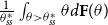 $\frac {1}{\theta _{ss}^{\ast }}\int _{\theta \gt \theta _{ss}^{\ast }}\theta d\mathbf{F}( \theta )$
in (24), keeping the cutoff
 $\theta _{ss}^{\ast }$
remained.Footnote
17
We find that the latter effect dominates the former effect such that
 $\mathbf{F}\big( \theta _{ss}^{\ast }\big) +\frac {1}{\theta _{ss}^{\ast }}\int _{\theta \gt \theta _{ss}^{\ast }}\theta d\mathbf{F}( \theta )$
rises as
 $v$
decreases. To uphold an equilibrium,
 $\theta _{ss}^{\ast }$
must increase in response to a lower
 $v$
, which serves as a counterbalancing force to offset the rise in
 $\mathbf{F}\big( \theta _{ss}^{\ast }\big) +\frac {1}{\theta _{ss}^{\ast }}\int _{\theta \gt \theta _{ss}^{\ast }}\theta d\mathbf{F}( \theta )$
in (24), caused by the decrease in
 $v$
.
Based on our theoretical findings, we identify three effects of
 $\tau _{ss}$
on
 $\bar {E}_{ss}$
: the direct effect, the threshold effect, and the income effect. To corroborate the theoretical findings, we evaluate the signs and magnitudes of the direct effect, the threshold effect, and the income effect. The quantitative results are presented in Figure 2. The solid line in Panel (a) holds
 $\bar {E}_{ss}$
fixed, computed under the baseline parameter values. As illustrated by the dotted line, an increase in
 $\tau _{ss}$
leads to greater tax evasion, capturing the direct effect. In contrast, the dashed and dash-dotted lines represent the threshold and income effects, respectively, both of which indicate a decline in tax evasion in response to a rise in
 $\tau _{ss}$
. Specifically, a higher
 $\tau _{ss}$
raises the cutoff
 $\theta _{ss}^{\ast }$
and reduces
 $x_{ss}$
, both of which exert downward pressure on
 $\bar {E}_{ss}$
, thereby partially offsetting the positive direct effect. Panel (b) illustrates
 $\bar {E}{ss}$
across varying values of
 $\tau {ss}$
, with the solid line representing the overall impact that incorporates all three effects. To isolate the effects of
 $ \tau _{ss}$
,
 $\theta _{ss}^{\ast }$
, and
 $x_{ss}$
, we hold each factor fixed one at a time. The dotted line shows that, when holding
 $\tau _{ss}=0.25$
, the underreported income is lower compared to the corresponding value under the overall effect. The vertical distance between the solid line and the dotted line, which results from the deviation of
 $\tau _{ss}$
from the baseline value
 $0.25$
, can be interpreted as the magnitude of the direct effect. Similarly, the vertical distance between the dashed line (dash-dotted line) and the solid line represents the threshold effect (the income effect). Note that when either
 $\theta _{ss}^{\ast }$
or
 $x_{ss}$
is fixed at their baseline values, i.e., as if determined under
 $\tau _{ss} = 0.25$
, the underreported income exceeds that under the overall effect.
Decomposing the effect of
 $ \tau _{ss}$
on
 $\bar {E}_{ss}$
.Note: In Panel (a), the solid line depicts
 $\bar {E}{ss}$
under the baseline parameters. We then illustrate how
 $\bar {E}{ss}$
responds to changes in
 $\tau _{ss}$
,
 $\theta _{ss}^{}$
, and
 $x$
individually, while holding the other factors fixed at their baseline levels. These are shown by the dotted line, the dashed line, and the dash-dotted line, respectively. In Panel (b), the solid line shows how
 $\bar {E}{ss}$
varies with changes in
 $\tau _{ss}$
. We then isolate the effect of each factor by holding
 $\tau _{ss}$
,
 $\theta _{ss}^{}$
, and
 $x$
fixed one at a time, depicted by the dotted line, the dashed line, and the dash-dotted line, respectively.

To further investigate how other parameters alter the relative sizes of the direct effect, the threshold effect, and the income effect, we rewrite (30) as
 \begin{equation} \frac {\bar {E}_{ss}}{x_{ss}}=\left ( \frac {1}{f}-\left ( \frac {1}{\tau _{ss}}+ \frac {1}{f}\right ) p\right ) \bar {\Gamma }\big( \theta _{ss}^{\ast }\big) , \end{equation}
where
 $\tau _{ss}$
influences
 $\frac {\bar {E}_{ss}}{x_{ss}}$
via two channels: the direct effect and the threshold effect.
From (30) and (35), we know
 $\tau _{ss}$
directly increases both
 $\bar {E}_{ss}$
and
 $\frac {\bar {E}_{ss}}{x_{ss}}$
, holding
 $\theta _{ss}^{\ast }$
and other variables fixed. Notably, a higher
 $p$
amplifies this positive direct effect. Put differently, the direct effect becomes stronger as
 $p$
increases.
Next, we examine the threshold effect, which dictates that
 $\tau _{ss}$
positively impacts the equilibrium cutoff
 $\theta _{ss}^{\ast }$
, which in turn reduces
 $\bar {E}_{ss}$
or
 $\frac {\bar {E}_{ss}}{x_{ss}}$
, given
 $\frac { \partial \bar {\Gamma }}{\partial \theta _{ss}^{\ast }}\lt 0$
. Recall from Proposition3 that the steady-state cutoff
 $\theta _{ss}^{\ast }$
increases in
 $\tau _{ss}$
. This occurs because a higher
 $\tau _{ss}$
, which pushed up
 $\bar {\Phi }$
, exerts downward pressure on the RHS of (E.1), resulting in a higher equilibrium cutoff
 $\theta _{ss}^{\ast }$
. By utilizing (C.1), we derive
 $\frac {\partial ^{2}\bar {\Phi }}{ \partial \tau _{ss}\partial p}\lt 0$
and
 $\frac {\partial ^{2}\bar {\Phi }}{ \partial \tau _{ss}\partial f}\lt 0$
. Consequently, while
 $\bar {\Phi }$
rises with
 $\tau _{ss}$
, this upward force diminishes as
 $p$
or
 $f$
increases, thus exerting less downward pressure on the RHS of (E.1). Therefore, we anticipate a weaker threshold effect when
 $p$
or
 $f$
is relatively high.
In summary, a positive effect of
 $\tau _{ss}$
on
 $\bar {E}_{ss}$
or
 $\frac { \bar {E}_{ss}}{x_{ss}}$
may emerge, provided that either
 $p$
or
 $f$
is sufficiently high. As depicted in Panel (a) of Figure 3, when
 $p$
and
 $f$
are set at 0.18 and 0.8, respectively,
 $\bar {E}_{ss}$
initially reacts positively to
 $\tau _{ss}$
and then declines as
 $\tau _{ss}$
increases. Meanwhile, Panel (b) of Figure 3 illustrates an upward trajectory of
 $\frac {\bar {E}_{ss}}{x_{ss}}$
as
 $\tau _{ss}$
rises.
Effects of
 $ \tau _{ss}$
on
 $\bar {E}_{ss}$
and
 $\frac {\bar {E} _{ss}}{x_{ss}}$
with
 $p=0.18$
and
 $f=0.8$
.

Decomposing the effect of
 $ \tau _{ss}$
on
 $\bar {E}_{ss}$
with
 $p=0.18$
and
 $f=0.8$
.Note: In Panel (a), the solid line depicts
 $\bar {E}{ss}$
under the baseline parameters. We then illustrate how
 $\bar {E}{ss}$
responds to changes in
 $\tau _{ss}$
,
 $\theta _{ss}^{}$
, and
 $x$
individually, while holding the other factors fixed at their baseline levels. These are shown by the dotted line, the dashed line, and the dash-dotted line, respectively. In Panel (b), the solid line shows how
 $\bar {E}{ss}$
varies with changes in
 $\tau _{ss}$
. We then isolate the effect of each factor by holding
 $\tau _{ss}$
,
 $\theta _{ss}^{}$
, and
 $x$
fixed one at a time, depicted by the dotted line, the dashed line, and the dash-dotted line, respectively.

Effects of
 $p$
on
 $ \theta _{ss}^{\ast }$
,
 $\bar {E}_{ss}$
, and
 $\frac {\bar {E}_{ss}}{x_{ss}}$
.

As shown in Panel (a) of Figure 4 where
 $p=0.18$
and
 $f=0.8$
, the total effect is decomposed into the three aforementioned components. Notably, the positive direct effect counteracts the negative threshold and income effects. Moreover, Panel (b) of Figure 4 indicates that the initial upward pattern of
 $\bar {E}_{ss}$
in response to an increase in
 $\tau _{ss}$
is driven by the relatively small magnitudes of the negative threshold and income effects. When combined with the positive direct effect, this results in an overall increase in
 $\bar {E}_{ss}$
as
 $\tau _{ss}$
rises. However, as
 $\tau _{ss}$
continues to increase, the threshold and income effects gradually outweigh the direct effect, leading to a decline in
 $\bar {E }_{ss}$
.Footnote
18
Recall that a higher
 $\tau _{ss}$
scales up
 $\theta _{ss}^{\ast }$
while scaling down
 $x_{ss}$
, thereby reinforcing the negative threshold and income effects. This example illustrates that increasing
 $p$
and
 $f$
, when
 $\tau _{ss}$
is not sufficiently large, leads to weaker threshold and income effects, which helps overturn the Yitzhaki puzzle.
Figure 5 reports how
 $\theta _{ss}^{\ast }$
,
 $\bar {E}_{ss}$
, and
 $\frac {\bar {E}_{ss}}{x_{ss}}$
, react to different values of the auditing probability,
 $p$
. As
 $p$
rises, both
 $\theta _{ss}^{\ast }$
and
 $\bar {E} _{ss}$
fall. As illustrated in Figure 6, similar patterns of
 $ \theta _{ss}^{\ast }$
,
 $\bar {E}_{ss}$
, and
 $\frac {\bar {E}_{ss}}{x_{ss}}$
, exist in response to rising
 $f$
. An implication drawn from these results is that a higher probability of tax detection or a higher penalty rate strengthens the effect of market incompleteness and borrowing limits on household decisions. In addition, individuals choose to underreport their income less if the cost of engaging in tax evasion rises. It is worth noting that the quantitative findings regarding
 $\theta _{ss}^{\ast }$
are consistent with our theoretical results of Proposition3.
Effects of
 $f$
on
 $ \theta _{ss}^{\ast }$
,
 $\bar {E}_{ss}$
, and
 $\frac {\bar {E}_{ss}}{x_{ss}}$
.

Next, we elaborate on the effects of
 $\eta$
and
 $b$
on
 $\theta _{ss}^{\ast }$
,
 $\bar {E}_{ss}$
, and
 $\frac {\bar {E}_{ss}}{x_{ss}}$
. As shown in Figure 7 and Figure 8,
 $\theta _{ss}^{\ast }$
decreases in
 $\eta$
and increases in
 $b$
.Footnote
19
Furthermore, despite a marginal increase in
 $\bar {E}_{ss}$
, individuals tend to underreport their income to a greater extent as borrowing limits become stricter. Conversely, when the government offers increased bond insurance, the level of tax evasion decreases. Upon examining these figures, it becomes evident that the patterns of
 $\theta _{ss}^{\ast }$
and
 $\bar {E}_{ss}$
persist regardless of the specific value of
 $v$
.
Effects of
 $ \eta$
on
 $ \theta _{ss}^{\ast }$
,
 $\bar { E}_{ss}$
, and
 $\frac {\bar {E}_{ss}}{x_{ss}}$
.

Effects of
 $b$
on
 $ \theta _{ss}^{\ast }$
,
 $\bar {E}_{ss}$
, and
 $\frac {\bar {E}_{ss}}{x_{ss}}$
.

Comparing panel (b) with panel (c) of Figure 7, we find the opposite trend of
 $\bar {E}_{ss}$
and
 $\frac {\bar {E}_{ss}}{x_{ss}}$
in response to changes in
 $\eta$
. To see that, by utilizing
 $\underline {a} =\eta x_{ss}$
with
 $\sigma =1$
, we rewrite the expression for
 $x_{ss}$
from Proposition1 as
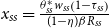 $x_{ss}=\frac { \theta _{ss}^{\ast }w_{ss}\left ( 1-\tau _{ss}\right ) }{ ( 1-\eta ) \beta R_{ss}}$
. Clearly, a higher
 $\eta$
increases
 $x_{ss}$
directly, while a reduction of
 $\theta _{ss}^{\ast }$
, driven by a greater
 $\eta$
, scales down
 $x_{ss}$
indirectly. Panel (c) in Figure 7 reveals that the direct effect outweighs the indirect effect. As such, since
 $x_{ss}$
increases in
 $\eta$
, we observe
 $\frac {\bar {E}_{ss}}{x_{ss}}$
declines as
 $ \eta$
rises.
We then examine how social welfare varies in response to changes in
 $f$
,
 $ \tau _{ss}$
, and
 $p$
, respectively. We present social welfare changes through consumption equivalent variation, measured as the percentage gain in consumption relative to the benchmark case. Utilizing (33), we impose the condition
 $SW_{ss}\left ( \left ( 1+\kappa \right ) \hat {c}_{ss}^{u},\left ( 1+\kappa \right ) \hat {c}_{ss}^{d},\hat {N}_{ss}\right ) =SW_{ss}\left ( \tilde {c }_{ss}^{u},\tilde {c}_{ss}^{d},\tilde {N}_{ss}\right )$
, where
 $\hat {c}$
and
 $ \hat {N}$
denote allocations derived under the baseline parameter values, and
 $\tilde {c}$
and
 $\tilde {N}$
denote allocations under the alternative parameter values for comparison. The values of
 $\kappa$
, interpreted as measures of relative welfare gain, are reported in Figure 9.
Optimal penalty rate

Steady-state welfare gain under varying
 $f$
,
 $ \tau _{ss}$
, and
 $p$
.Note: The benchmark scenario is identified by an asterisk.

As shown in panel (a) of Figure 9, the steady-state welfare gain initially increases in
 $f$
and then declines in
 $f$
. In this benchmark case, there exists
 $f^{\ast }=0.375$
, which maximizes the steady-state welfare gain found in Table 2. Table 2 also reports the optimal penalty rates for various scenarios, each permitting a single parameter to vary from its baseline value. We find that
 $f^{\ast }$
decreases in
 $p$
or
 $v$
, and increases in
 $\tau _{ss}$
. The intuition is as follows. A rise in either
 $p$
or
 $v$
results in a lower
 $\theta _{ss}^{\ast }$
, which means more financially constrained individuals. As such, the social planner lowers the optimal penalty rate so as to raise
 $\theta _{ss}^{\ast }$
. Likewise, a rise in
 $\tau _{ss}$
leads to a higher
 $\theta _{ss}^{\ast }$
. Therefore, in order to counteract the positive effect of
 $ \tau _{ss}$
on
 $\theta _{ss}^{\ast }$
, the social planner increases the optimal penalty rate. The reaction of
 $f^{\ast }$
to changes in
 $p$
,
 $v$
, or
 $\tau _{ss}$
is primarily driven by the social planner’s desire to offset the effect of changes in
 $p$
,
 $v$
, or
 $\tau _{ss}$
on
 $\theta _{ss}^{\ast }$
. Whereas, this rationale cannot be applied to the cases where either
 $\eta$
or
 $b$
increases. It can be seen that the effect of a rising
 $\eta$
and the effect of a higher
 $f$
on
 $\theta _{ss}^{\ast }$
are both negative. Meanwhile, the effect of a rising
 $b$
and the effect of a lower
 $f$
on
 $ \theta _{ss}^{\ast }$
are both positive. Thus, the force that drives
 $ f^{\ast }$
to deviate from
 $0.375$
does not stem from the motive to restore the original
 $\theta _{ss}^{\ast }$
. Instead, the force is associated with the change in capital which is triggered by the change in the asset market. A higher
 $\eta$
means that individuals facing a tighter borrowing limit have to save more, which boosts investment at steady state. On the other hand, a greater
 $b$
implies a higher demand for loanable funds, which in turn crowds out the formation of physical capital. In response to higher (lower) capital accumulated and thus higher (lower) output/income, the social planner chooses to raise (reduce) the optimal penalty rate.
We also present the relationship between the steady-state welfare gain and
 $ \tau _{ss}\left ( p\right )$
. Panels (b) and (c) of Figure 9 reveal that the steady-state welfare gain decreases as either
 $\tau _{ss}$
or
 $p$
increases, holding the other parameters’ values unchanged. Recall the result of Proposition3 that raising
 $\tau _{ss}$
helps relax the borrowing constraints, thereby reducing the fraction of the population facing the binding borrowing constraints becomes less. However, this relaxation comes at the expense of shrinking output and income. Clearly, the cost outweighs the benefit, given the other parameters’ values. Similarly, according to Proposition3, as
 $p$
falls, the cutoff
 $\theta _{ss}^{\ast }$
increases, resulting in a welfare improvement in the steady state.
Lastly, we report Gini coefficients of consumption under different scenarios regarding varying
 $\tau _{ss}$
,
 $f$
, and
 $p$
.Footnote
20
Since this tractable model eliminates the wealth-redistribution effect and maintains a degenerate wealth distribution, we focus on the Gini coefficient of consumption to examine the extent of inequality in the economy. As shown in Figure 10, the Gini coefficient for consumption rises with an increase in
 $\tau _{ss}$
but declines as
 $f$
and
 $p$
increase. In addition, the cutoff
 $\theta _{ss}^{\ast }$
also rises with
 $\tau _{ss}$
and falls as
 $f$
and
 $p$
increase. This relationship highlights the trade-off between allocative efficiency and redistribution.
Gini Coefficients under varying
 $ \tau$
,
 $f$
, and
 $p$
.

6. Conclusion
This paper, extending seminal works by Allingham and Sandmo (Reference Allingham and Sandmo1972) and Yitzhaki (Reference Yitzhaki1974), analyzes the intricate relationship between tax evasion and tax rates within a heterogeneous-agent incomplete-markets model. We elucidate how financially constrained households strategically employ tax evasion to counter the impact of financial market imperfections, shedding light on tax evasion as a risk-mitigating strategy for such households. Our analysis highlights that policy instruments designed to deter tax evasion, such as the probability of auditing and the penalty rate, exacerbate the effects of borrowing constraints on household decisions. Crucially, we unveil that when tax evasion is endogenous, an increase in the income tax rate mitigates the adverse impact of borrowing constraints. In particular, our numerical insights offer novel perspectives on the Yitzhaki puzzle, indicating an initial increase in underreported income with rising tax rates, followed by a subsequent decline.
We exploit our theoretical results to explore the factors underlying the Yitzhaki puzzle. Indeed, unlike the Aiyagari model, this framework leads to a degenerate wealth distribution among individuals, excluding any redistribution effects linked to tax evasion. However, in the absence of these effects, we are able to accentuate the linkage between tax evasion and the severity of financial market friction, captured by
 $\theta _{ss}^{\ast }$
. In particular, we place emphasis on how tax evasion enhances individuals’ self-insurance, thereby improving aggregate allocative efficiency.
At the steady state, the issuance of government bonds alleviates borrowing constraints by reducing the fraction of individuals facing binding limits. In contrast, when borrowing constraints tighten, a larger share of individuals becomes financially constrained. Our numerical analysis also indicates that a higher audit probability increases the number of constrained individuals, prompting the social planner to lower the optimal penalty rate to offset this negative impact. Conversely, an increase in the income tax rate reduces the incidence of financial constraints, leading the planner to raise the optimal penalty rate. These findings underscore the nuanced interactions between tax evasion, financial frictions, and policy instruments.
This tractable model can be extended in several dimensions. Firstly, the work of Gahvari and Micheletto (Reference Gahvari and Micheletto2014) demonstrated that income tax evasion leads to the violation of the Friedman rule in an overlapping-generations economy. However, Gahvari and Micheletto (Reference Gahvari and Micheletto2014) did not consider idiosyncratic shocks in an incomplete-markets economy. Our model, which shows that tax evasion acts as a strategy for financially constrained households to mitigate the adverse impacts of financial market imperfections, can be extended by incorporating overlapping generations and money. Secondly, this paper focuses solely on labor income taxation. It would be interesting to explore the effects of capital taxation on the severity of financial market imperfections when tax evasion is an endogenous choice.
Acknowledgments
The authors would like to thank the anonymous Associate Editor and the two anonymous referees for their helpful comments and suggestions. Yunmin Chen gratefully acknowledges financial support from Taiwan National Science and Technology Council (NSTC 112-2410-H-008-075).
Competing interests
The authors declare that they have no competing interests.
A. Proof of Proposition1
To prove Proposition1, we outline the procedures step by step, beginning with the establishment of the following lemmas.
1. We characterize
 $\left \{ \lambda _{t}^{d}( \theta ^{t}) \right \} _{t=0}^{\infty }$
for each shock realization history.
Lemma 1.
The gross income and the Lagrange multiplier,
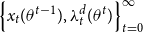 $\left \{ x_{t}( \theta ^{t-1}) ,\lambda _{t}^{d}( \theta ^{t}) \right \} _{t=0}^{\infty }$
, satisfy
 \begin{align}& x_{t}=\underline {a}+\left ( \frac {\theta _{t}^{\ast }}{\frac {\beta R_{t+1}}{ w_{t+1}\left ( 1-\tau _{t+1}\right ) }\frac {1}{\frac {f}{\tau _{t}}+1}}\right ) ^{\frac {1}{\sigma }}\left [ \frac {\tau _{t}}{f+\tau _{t}}p^{\frac {1}{\sigma } }+\left ( 1-\frac {\tau _{t}}{f+\tau _{t}}\right ) \left ( \frac {\tau _{t} ( 1-p) }{f}\right ) ^{\frac {1}{\sigma }}\right ] . \end{align}
 \begin{align}&\qquad\qquad\qquad \lambda _{t}^{d} ( \theta _{t}) =\Lambda _{t}=\frac {\beta R_{t+1}}{ w_{t+1}\left ( 1-\tau _{t+1}\right ) }\frac {1}{\frac {f}{\tau _{t}}+1}\text{ for }\theta _{t}\leq \theta _{t}^{\ast }, \end{align}
 \begin{align}&\qquad\qquad\qquad\,\, \lambda _{t}^{d} ( \theta _{t}) =\frac {\theta _{t}}{\theta _{t}^{\ast }}\frac {\beta R_{t+1}}{w_{t+1}\left ( 1-\tau _{t+1}\right ) }\frac {1 }{\frac {f}{\tau _{t}}+1}\text{ for }\theta _{t}\gt \theta _{t}^{\ast }. \end{align}
Proof. Firstly, plugging (12) into (11) and (13) gives rise to
 \begin{align}&\quad \frac {1}{w_{t} ( 1-\tau _{t}) \left ( \frac {f}{\tau _{t}}+1\right ) } =\int \lambda _{t}^{d}( \theta ^{t}) d\mathbf{F} ( \theta _{t}) , \end{align}
 \begin{align}& \frac {\beta R_{t+1}}{w_{t+1}\left ( 1-\tau _{t+1}\right ) }+\mu _{t}( \theta ^{t}) =\left ( \frac {f}{\tau _{t}}+1\right ) \lambda _{t}^{d}( \theta ^{t}) , \end{align}
which is derived by the law of iterative expectation and the assumption of an i.i.d. shock process.
Next, we employ a “guess-and-verify” approach to formulate the decision rules. The individual’s consumption and saving rules follow a cutoff strategy, determined by the state
 $\left ( w_{t},R_{t+1},\tau _{t},\tau _{t+1},f\right )$
. Considering the anticipation that the optimal cutoff
 $\theta _{t}^{\ast }$
remains unaffected by an individual’s past shock history, we contemplate two potential scenarios:
Case A:
 $\theta _{t}\leq \theta _{t}^{\ast }$
. In this case, the propensity to consume is so low that the borrowing constraint is not binding. As such, we have
 $a_{t+1}( \theta ^{t}) \geq \underline {a }$
and
 $\mu _{t}( \theta ^{t}) =0$
. In light of (A.5), we know
 $\lambda _{t}^{d}( \theta ^{t})$
only depends on the aggregate state and irrelevant to the history
 $\theta ^{t}$
. Therefore, we re-express (A.5) as
 \begin{equation} \frac {\beta R_{t+1}}{w_{t+1}\left ( 1-\tau _{t+1}\right ) }=\left ( \frac {f}{ \tau _{t}}+1\right ) \lambda _{t}^{d}( \theta ^{t}) \equiv \left ( \frac {f}{\tau _{t}}+1\right ) \Lambda _{t}. \end{equation}
By (9), (10), and (12), we obtain
 \begin{eqnarray*} ( 1-p) \theta _{t}c_{t}^{u}( \theta ^{t}) ^{-\sigma } &=&\lambda _{t}^{u}( \theta ^{t}) \\ &=&\frac {f}{\tau _{t}}\lambda _{t}^{d}( \theta ^{t}) \\ &=&\frac {f}{\tau _{t}}\Lambda _{t}, \end{eqnarray*}
 \begin{equation*} p\theta _{t}c_{t}^{d}( \theta ^{t}) ^{-\sigma }=\lambda _{t}^{d}( \theta ^{t}) =\Lambda _{t}, \end{equation*}
which can be simplified as
 \begin{align}& c_{t}^{u} ( \theta _{t}) ^{\sigma }=\frac { ( 1-p) \theta _{t}}{\frac {f}{\tau _{t}}\Lambda _{t}}, \end{align}
 \begin{align}&\quad c_{t}^{d} ( \theta _{t}) ^{\sigma }=\frac {p\theta _{t}}{\Lambda _{t}}. \end{align}
Turning to the asset holdings, we utilize flow budget constraints (5) and (6), with (A.7) and (A.8), to rewrite them as
 \begin{eqnarray} a_{t+1}( \theta ^{t}) &=&x_{t}( \theta ^{t-1}) +\tau _{t}E_{t}( \theta ^{t}) -c_{t}^{u} ( \theta _{t}) \notag \\ &=&x_{t}( \theta ^{t-1}) +\tau _{t}E_{t}( \theta ^{t}) -\left ( \frac { ( 1-p) \theta _{t}}{\frac {f}{\tau _{t}}\Lambda _{t}} \right ) ^{\frac {1}{\sigma }}, \end{eqnarray}
 \begin{eqnarray} a_{t+1}( \theta ^{t}) &=&x_{t}( \theta ^{t-1}) -fE_{t}( \theta ^{t}) -c_{t}^{d}( \theta ^{t}) \notag \\ &=&x_{t}( \theta ^{t-1}) -fE_{t}( \theta ^{t}) -\left ( \frac {p\theta _{t}}{\Lambda _{t}}\right ) ^{\frac {1}{\sigma }}. \end{eqnarray}
From (A.9) and (A.10), we solve for
 $E_{t}( \theta ^{t})$
:
 \begin{eqnarray} E_{t}( \theta ^{t}) &=&\frac {1}{f+\tau _{t}}\left [ \left ( \frac { ( 1-p) \theta _{t}}{\frac {f}{\tau _{t}}\Lambda _{t}}\right ) ^{\frac {1}{\sigma }}-\left ( \frac {p\theta _{t}}{\Lambda _{t}}\right ) ^{\frac {1 }{\sigma }}\right ] \notag \\ &=&\frac {1}{f+\tau _{t}}\left ( \frac {\theta _{t}}{\Lambda _{t}}\right ) ^{ \frac {1}{\sigma }}\left [ \left ( \frac {\tau _{t} ( 1-p) }{f}\right ) ^{\frac {1}{\sigma }}-p^{\frac {1}{\sigma }}\right ] . \end{eqnarray}
Inserting (A.11) into (A.9) yields
 \begin{eqnarray*} a_{t+1}( \theta ^{t}) &=&x_{t}( \theta ^{t-1}) -\frac { \tau _{t}}{f+\tau _{t}}\left ( \frac {\theta _{t}}{\Lambda _{t}}\right ) ^{ \frac {1}{\sigma }}\left [ p^{\frac {1}{\sigma }}-\left ( \frac {\tau _{t} ( 1-p) }{f}\right ) ^{\frac {1}{\sigma }}\right ] -\left ( \frac { ( 1-p) \theta _{t}}{\frac {f}{\tau _{t}}\Lambda _{t}}\right ) ^{\frac {1}{ \sigma }} \\ &=&x_{t}( \theta ^{t-1}) -\left ( \frac {\theta _{t}}{\Lambda _{t}} \right ) ^{\frac {1}{\sigma }}\left [ \frac {\tau _{t}}{f+\tau _{t}}p^{\frac {1}{ \sigma }}+\frac {f}{f+\tau _{t}}\left ( \frac {\tau _{t} ( 1-p) }{f} \right ) ^{\frac {1}{\sigma }}\right ] . \end{eqnarray*}
Given
 $a_{t+1}( \theta ^{t}) \geq \underline {a}$
, we have
 \begin{equation*} x_{t}( \theta ^{t-1}) -\left ( \frac {\theta _{t}}{\Lambda _{t}} \right ) ^{\frac {1}{\sigma }}\left [ \frac {\tau _{t}}{f+\tau _{t}}p^{\frac {1}{ \sigma }}+\frac {f}{f+\tau _{t}}\left ( \frac {\tau _{t} ( 1-p) }{f} \right ) ^{\frac {1}{\sigma }}\right ] \geq \underline {a}. \end{equation*}
Alternatively, we obtain
 \begin{equation} \theta _{t}\leq \frac {\left ( x_{t}( \theta ^{t-1}) -\underline {a} \right ) ^{\sigma }\Lambda _{t}}{\left [ \frac {\tau _{t}}{f+\tau _{t}}p^{\frac { 1}{\sigma }}+\frac {f}{f+\tau _{t}}\left ( \frac {\tau _{t} ( 1-p) }{f }\right ) ^{\frac {1}{\sigma }}\right ] ^{\sigma }}\equiv \theta _{t}^{\ast }, \text{ and} \end{equation}
 \begin{equation*} x_{t}( \theta ^{t-1}) =\underline {a}+\left ( \frac {\theta _{t}^{\ast }}{\frac {\beta R_{t+1}}{w_{t+1}\left ( 1-\tau _{t+1}\right ) }\frac { 1}{\frac {f}{\tau _{t}}+1}}\right ) ^{\frac {1}{\sigma }}\left [ \frac {\tau _{t} }{f+\tau _{t}}p^{\frac {1}{\sigma }}+\frac {f}{f+\tau _{t}}\left ( \frac {\tau _{t} ( 1-p) }{f}\right ) ^{\frac {1}{\sigma }}\right ] , \end{equation*}
which implies that
 $x_{t}( \theta ^{t-1})$
is independent of
 $ \theta ^{t-1}$
; hence we succinctly write down
 $x_{t}$
rather than
 $ x_{t}( \theta ^{t-1})$
.
Case B:
 $\theta _{t}\gt \theta _{t}^{\ast }$
. In this case, the desire to consume is so high that individuals are compelled to borrow, ultimately reaching their borrowing limits. Therefore, we have
 $a_{t+1}( \theta ^{t}) =\underline {a}$
and
 $\mu _{t}( \theta ^{t}) \gt 0$
.
By
 $a_{t+1}( \theta ^{t}) =\underline {a}$
, (9), and (10), we rewrite (5) and (6) as
 \begin{eqnarray} x_{t}+\tau _{t}E_{t}( \theta ^{t}) &=&\left ( \frac {\lambda _{t}^{u}( \theta ^{t}) }{ ( 1-p) \theta _{t}}\right ) ^{ \frac {-1}{\sigma }}+\underline {a} \notag \\ &=&\left ( \frac {f}{\tau _{t} ( 1-p) \theta _{t}}\lambda _{t}^{d}( \theta ^{t}) \right ) ^{\frac {-1}{\sigma }}+\underline {a} , \end{eqnarray}
 \begin{equation} x_{t}-fE_{t}( \theta ^{t}) =\left ( \frac {\lambda _{t}^{d}( \theta ^{t}) }{p\theta _{t}}\right ) ^{\frac {-1}{\sigma }}+\underline {a} . \end{equation}
Similarly, we solve for
 $E_{t}( \theta ^{t})$
from (A.13) and (A.14):
 \begin{equation} E_{t}( \theta ^{t}) =\frac {1}{f+\tau _{t}}\left [ \left ( \frac {f}{ \tau _{t} ( 1-p) \theta _{t}}\right ) ^{\frac {-1}{\sigma }}-\left ( \frac {1}{p\theta _{t}}\right ) ^{\frac {-1}{\sigma }}\right ] \left ( \lambda _{t}^{d}( \theta ^{t}) \right ) ^{\frac {-1}{\sigma }}. \end{equation}
Plugging (A.1) and (A.15) back to (A.13) gives
 \begin{equation} \lambda _{t}^{d}( \theta ^{t}) =\frac {\theta _{t}}{\theta _{t}^{\ast }}\frac {\beta R_{t+1}}{w_{t+1}\left ( 1-\tau _{t+1}\right ) }\frac {1 }{\frac {f}{\tau _{t}}+1}. \end{equation}
Combining case A and case B, we derive (A.2) and (A.3). Notice that from (A.16), we have
 $\lambda _{t}^{d}( \theta ^{t}) =$
 $\lambda _{t}^{d} ( \theta _{t}) ,\forall \theta ^{t}$
.
2. We characterize
 $\left \{ c_{t}^{u}( \theta ^{t}) ,c_{t}^{d}( \theta ^{t}) \right \} _{t=0}^{\infty }$
for each shock realization history.
Lemma 2.
The decision rules of consumption,
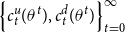 $\left \{ c_{t}^{u}( \theta ^{t}) ,c_{t}^{d}( \theta ^{t}) \right \} _{t=0}^{\infty }$
, are given by
 \begin{align} c_{t}^{u} ( \theta _{t}) =\left ( \frac {\tau _{t} ( 1-p) }{f}\frac {\theta _{t}}{\theta _{t}^{\ast }}\frac {\theta _{t}^{\ast }}{ \Lambda _{t}}\right ) ^{\frac {1}{\sigma }}=\left ( \frac {\theta _{t}}{\theta _{t}^{\ast }}\right ) ^{\frac {1}{\sigma }} ( x_{t}-\underline {a}) \kappa _{t}^{u},\text{ for }\theta _{t}\leq \theta _{t}^{\ast }, \end{align}
 \begin{align} c_{t}^{d} ( \theta _{t}) =\left ( p\frac {\theta _{t}}{\theta _{t}^{\ast }}\frac {\theta _{t}^{\ast }}{\Lambda _{t}}\right ) ^{\frac {1}{ \sigma }}=\left ( \frac {\theta _{t}}{\theta _{t}^{\ast }}\right ) ^{\frac {1}{ \sigma }} ( x_{t}-\underline {a}) \kappa _{t}^{d},\text{ for } \theta _{t}\leq \theta _{t}^{\ast }, \end{align}
 \begin{align} c_{t}^{u} ( \theta _{t}) = ( x_{t}-\underline {a}) \kappa _{t}^{u},\text{ for }\theta _{t}\gt \theta _{t}^{\ast }, \end{align}
 \begin{align}&\qquad\qquad\qquad\quad c_{t}^{d} ( \theta _{t}) = ( x_{t}-\underline {a}) \kappa _{t}^{d},\text{ for }\theta _{t}\gt \theta _{t}^{\ast }, \end{align}
Proof. For
 $\theta _{t}\leq \theta _{t}^{\ast }$
, we use (A.7), (A.8 ), (A.12), and (A.2) to derive (A.17) and (A.18).
By (5), (6), and (A.15) with
 $a_{t+1}( \theta ^{t}) =\underline {a}$
, we back out
 $c_{t}^{u}( \theta ^{t})$
and
 $c_{t}^{d}( \theta ^{t})$
for
 $\theta _{t}\gt \theta _{t}^{\ast }$
:
 \begin{align} c_{t}^{u}( \theta ^{t}) =x_{t}-\underline {a}+\frac {\tau _{t}}{ f+\tau _{t}}\left [ \left ( \frac {\tau _{t} ( 1-p) }{f}\right ) ^{ \frac {1}{\sigma }}-p^{\frac {1}{\sigma }}\right ] \left ( \frac {1}{\theta _{t}^{\ast }}\frac {\beta R_{t+1}}{w_{t+1}\left ( 1-\tau _{t+1}\right ) }\frac {\tau _{t}}{f+\tau _{t}}\right ) ^{\frac {-1}{\sigma }}, \end{align}
 \begin{align}c_{t}^{d}( \theta ^{t}) =x_{t}-\underline {a}-\frac {f}{f+\tau _{t}} \left [ \left ( \frac {\tau _{t} ( 1-p) }{f}\right ) ^{\frac {1}{\sigma }}-p^{\frac {1}{\sigma }}\right ] \left ( \frac {1}{\theta _{t}^{\ast }}\frac { \beta R_{t+1}}{w_{t+1}\left ( 1-\tau _{t+1}\right ) }\frac {\tau _{t}}{f+\tau _{t}}\right ) ^{\frac {-1}{\sigma }}, \end{align}
where we employ (A.16). Substituting (A.6) and (A.12) into (A.21) and (A.22) gives (A.19) and (A.20 ).Clearly, for
 $\theta _{t}\leq \theta _{t}^{\ast }$
, the values of
 $ c_{t}^{u}( \theta ^{t})$
and
 $c_{t}^{d}( \theta ^{t})$
are contingent upon
 $\theta _{t}$
but remain unaffected by
 $\theta ^{t-1}$
. For
 $\theta _{t}\gt \theta _{t}^{\ast }$
, the decisions for
 $c_{t}^{u}( \theta ^{t})$
and
 $c_{t}^{d}( \theta ^{t})$
solely hinge upon the aggregate state.
3. We characterize
 $\left \{ E_{t}( \theta ^{t}) \right \} _{t=0}^{\infty }$
for each shock realization history.
Lemma 3.
The decision rule of income underreport,
 $\left \{ E_{t}( \theta ^{t}) \right \} _{t=0}^{\infty }$
, is given by
 \begin{align}& \left ( f+\tau _{t}\right ) E_{t} ( \theta _{t}) =\left ( \frac { \theta _{t}}{\theta _{t}^{\ast }}\right ) ^{\frac {1}{\sigma }}\left ( x_{t}- \underline {a}\right ) \big( \kappa _{t}^{u}-\kappa _{t}^{d}\big) ,\text{ for }\theta _{t}\leq \theta _{t}^{\ast }, \end{align}
 \begin{align}&\qquad \left ( f+\tau _{t}\right ) E_{t} ( \theta _{t}) =\left ( x_{t}- \underline {a}\right ) \big( \kappa _{t}^{u}-\kappa _{t}^{d}\big) ,\text{ for }\theta _{t}\gt \theta _{t}^{\ast }. \end{align}
Proof. Rewrite (A.11) as
 \begin{eqnarray*} \left ( f+\tau _{t}\right ) E_{t}( \theta ^{t}) &=&\left ( \frac { \theta _{t}}{\theta _{t}^{\ast }}\right ) ^{\frac {1}{\sigma }}\left ( \frac { \theta _{t}^{\ast }}{\Lambda _{t}}\right ) ^{\frac {1}{\sigma }}\left [ \left ( \frac {\tau _{t} ( 1-p) }{f}\right ) ^{\frac {1}{\sigma }}-p^{\frac {1 }{\sigma }}\right ] \\ &=&\left ( \frac {\theta _{t}}{\theta _{t}^{\ast }}\right ) ^{\frac {1}{\sigma } } ( x_{t}-\underline {a}) \big( \kappa _{t}^{u}-\kappa _{t}^{d}\big) ,\text{for }\theta _{t}\leq \theta _{t}^{\ast }, \end{eqnarray*}
where the second line comes from (A.12).
Similarly, given by (A.12), (A.15), and (A.16), we derive (A.24).
Notice that for
 $\theta _{t}\leq \theta _{t}^{\ast }$
, the levels of
 $ E_{t}( \theta ^{t})$
are determined by
 $\theta _{t}$
, rather than the past history of shock realizations,
 $\theta ^{t-1}$
. For
 $\theta _{t}\gt \theta _{t}^{\ast }$
, the decisions on income underreported
 $ E_{t}( \theta ^{t})$
are solely dependent on the aggregate state.
4. We characterize
 $\left \{ a_{t+1}( \theta ^{t}) \right \} _{t=0}^{\infty }$
for each shock realization history.
Lemma 4.
The decision rule of savings,
 $\left \{ a_{t+1}( \theta ^{t}) \right \} _{t=0}^{\infty }$
, is given by
 \begin{equation} a_{t+1} ( \theta _{t}) =x_{t}-\left ( \frac {\theta _{t}}{\theta _{t}^{\ast }}\right ) ^{\frac {1}{\sigma }} ( x_{t}-\underline {a}) , \text{for }\theta _{t}\leq \theta _{t}^{\ast }\text{, and} \end{equation}
 \begin{equation*} a_{t+1}( \theta ^{t}) =\underline {a}\text{for}\theta _{t}\gt \theta _{t}^{\ast }. \end{equation*}
Proof. We utilize (5), (A.11), (A.12), and (A.17) to derive
 \begin{eqnarray*} a_{t+1}( \theta ^{t}) &=&x_{t}+\tau _{t}E_{t}( \theta ^{t}) -c_{t}^{u}( \theta ^{t}) \\ &=&x_{t}+\frac {\tau _{t}}{f+\tau _{t}}\left ( \frac {\theta _{t}}{\Lambda _{t}} \right ) ^{\frac {1}{\sigma }}\left [ \left ( \frac {\tau _{t} ( 1-p) }{ f}\right ) ^{\frac {1}{\sigma }}-p^{\frac {1}{\sigma }}\right ] -\left ( \frac { \theta _{t}}{\theta _{t}^{\ast }}\right ) ^{\frac {1}{\sigma }}\left ( x_{t}- \underline {a}\right ) \kappa _{t}^{u} \\ &=&x_{t}+\frac {\tau _{t}}{f+\tau _{t}}\left ( \frac {\theta _{t}}{\theta _{t}^{\ast }}\right ) ^{\frac {1}{\sigma }}\left ( \frac {\theta _{t}^{\ast }}{ \Lambda _{t}}\right ) ^{\frac {1}{\sigma }}\left [ \left ( \frac {\tau _{t} ( 1-p) }{f}\right ) ^{\frac {1}{\sigma }}-p^{\frac {1}{\sigma }}\right ] \\ &&-\left ( \frac {\theta _{t}}{\theta _{t}^{\ast }}\right ) ^{\frac {1}{\sigma } } ( x_{t}-\underline {a}) \kappa _{t}^{u} \\ &=&x_{t}+\left ( \frac {\theta _{t}}{\theta _{t}^{\ast }}\right ) ^{\frac {1}{ \sigma }} ( x_{t}-\underline {a}) \frac {\frac {\tau _{t}}{f+\tau _{t} }\left [ \left ( \frac {\tau _{t} ( 1-p) }{f}\right ) ^{\frac {1}{ \sigma }}-p^{\frac {1}{\sigma }}\right ] }{\frac {f}{f+\tau _{t}}\left ( \frac { \tau _{t} ( 1-p) }{f}\right ) ^{\frac {1}{\sigma }}+\frac {\tau _{t}}{ f+\tau _{t}}p^{\frac {1}{\sigma }}} \\ &&-\left ( \frac {\theta _{t}}{\theta _{t}^{\ast }}\right ) ^{\frac {1}{\sigma } } ( x_{t}-\underline {a}) \frac {\left ( \frac {\tau _{t} ( 1-p) }{f}\right ) ^{\frac {1}{\sigma }}}{\frac {f}{f+\tau _{t}}\left ( \frac {\tau _{t} ( 1-p) }{f}\right ) ^{\frac {1}{\sigma }}+\frac {\tau _{t}}{f+\tau _{t}}p^{\frac {1}{\sigma }}} \\ &=&x_{t}-\left ( \frac {\theta _{t}}{\theta _{t}^{\ast }}\right ) ^{\frac {1}{ \sigma }} ( x_{t}-\underline {a}) \text{, for }\theta _{t}\leq \theta _{t}^{\ast }\text{.} \end{eqnarray*}
For
 $\theta _{t}\gt \theta _{t}^{\ast }$
,
 $a_{t+1}( \theta ^{t})$
is restricted to
 $a$
. It is evident that the level of
 $ a_{t+1}( \theta ^{t})$
is only determined by the current shock realization
 $\theta _{t}$
, and is irrelevant to the past history of shock realizations,
 $\theta ^{t-1}$
.
5. We pin down the cutoff
 $\theta _{t}^{\ast }$
by substituting (A.2)–(A.3) into (A.4) deriving
 \begin{eqnarray} \frac {1}{w_{t} ( 1-\tau _{t}) \left ( \frac {f}{\tau _{t}}+1\right ) } &=&\int _{\theta \leq \theta _{t}^{\ast }}\lambda _{t}^{d}( \theta )\; d\mathbf{F}( \theta ) +\int _{\theta \gt \theta _{t}^{\ast }}\lambda _{t}^{d}( \theta )\; d\mathbf{F}( \theta ) \notag \\ &=&\frac {\beta R_{t+1}}{w_{t+1}\left ( 1-\tau _{t+1}\right ) }\frac {1}{\frac {f }{\tau _{t}}+1}\left ( \mathbf{F}\big ( \theta _{t}^{\ast }\big) +\int _{\theta \gt \theta _{t}^{\ast }}\frac {\theta }{\theta _{t}^{\ast }}d \mathbf{F}( \theta ) \right ) , \end{eqnarray}
which is the Euler equation. As indicated in (A.26), the cutoff
 $ \theta _{t}^{\ast }$
is determined by
 $w_{t},w_{t+1},\tau _{t},\tau _{t+1},$
and
 $R_{t+1}$
.
6. Lastly,
 $n_{t}\left ( \theta _{t-1}\right ) =\frac {x_{t}-R_{t}a_{t} \left ( \theta _{t-1}\right ) }{ ( 1-\tau _{t}) w_{t}}$
is obtained by rearranging the definition of
 $x_{t}$
.
We complete the description of allocations
 $\left \{ c_{t}^{u}( \theta ^{t}) ,c_{t}^{d}( \theta ^{t}) \right \} _{t=0}^{\infty },\left \{ E_{t}( \theta ^{t}) \right \} _{t=0}^{\infty },\left \{ a_{t+1}( \theta ^{t}) \right \} _{t=0}^{\infty }, \left \{ n_{t}\left ( \theta _{t-1}\right ) \right \} _{t=1}^{\infty }$
, and the cutoff
 $ \left \{ \theta _{t}^{\ast }\right \} _{t=0}^{\infty }$
for the economy. The proof comes from lemmas2, 3, and 4, in conjunction with (A.26) and the expression
 $n_{t}\left ( \theta _{t-1}\right ) =\frac {x_{t}-R_{t}a_{t}\left ( \theta _{t-1}\right ) }{ ( 1-\tau _{t}) w_{t}}$
.
B. Proof of Proposition2
We begin the proof by deriving the expression for
 $R_{ss}$
. Then, using the Euler equation, which depends on
 $R_{ss}$
, we identify
 $\theta _{ss}^{\ast }$
.
Firstly, to determine
 $R_{ss}$
, we solve for
 $\left \{ K_{ss},N_{ss},C_{ss}\right \}$
from the following three equations:
 \begin{align} \left ( 1-g\right ) K_{ss}^{\alpha }N_{ss}^{1-\alpha }=\delta K_{ss}+C_{ss}, \end{align}
 \begin{align} C_{ss}=\frac {p^{\frac {1+\sigma }{\sigma }}+ ( 1-p) \left ( \frac { \tau _{ss} ( 1-p) }{f}\right ) ^{\frac {1}{\sigma }}}{\frac {f}{ f+\tau _{ss}}\left ( \frac {\tau _{ss} ( 1-p) }{f}\right ) ^{\frac {1}{ \sigma }}+\frac {\tau _{ss}}{f+\tau _{ss}}p^{\frac {1}{\sigma }}}x_{ss}\left [ \int _{\theta \leq \theta _{ss}^{\ast }}\left ( \frac {\theta }{\theta _{ss}^{\ast }}\right ) ^{\frac {1}{\sigma }}d\mathbf{F}( \theta ) +1-\mathbf{F}\big( \theta _{ss}^{\ast }\big) \right ] , \end{align}
 \begin{align} K_{ss}=x_{ss}\left [ \mathbf{F}\big( \theta _{ss}^{\ast }\big) -\int _{\theta \leq \theta _{ss}^{\ast }}\left ( \frac {\theta }{\theta _{ss}^{\ast }}\right ) ^{\frac {1}{\sigma }}d\mathbf{F}( \theta ) \right ] , \end{align}
where (B.1), (B.2), and (B.3) are the steady-state version of (8), (22), and (23) with
 $\underline {a}=0$
,
 $B_{ss}=0$
, and
 $G_{ss}=gK_{ss}^{\alpha }N_{ss}^{1-\alpha }$
imposed.
Next, we rewrite (B.1) as
 \begin{equation} \left ( 1-g\right ) \left ( \frac {K_{ss}}{N_{ss}}\right ) ^{\alpha -1}=\delta + \frac {C_{ss}}{K_{ss}}. \end{equation}
Subsequently, substituting (B.2) and (B.3) into (B.4) leads to
 \begin{equation} \frac {K_{ss}}{N_{ss}}=\left ( \frac {1}{1-g}\right ) ^{\frac {1}{\alpha -1}} \left [ \delta +\frac {\Phi \left [ \frac {v\sigma }{1-v\sigma }\left [ \left ( \frac {\theta _{L}}{\theta _{ss}^{\ast }}\right ) ^{v}-\left ( \frac {\theta _{L} }{\theta _{ss}^{\ast }}\right ) ^{\frac {1}{\sigma }}\right ] +\left ( \frac { \theta _{L}}{\theta _{ss}^{\ast }}\right ) ^{v}\right ] }{1-\left ( \frac { \theta _{L}}{\theta _{ss}^{\ast }}\right ) ^{v}-\frac {v\sigma }{1-v\sigma } \left [ \left ( \frac {\theta _{L}}{\theta _{ss}^{\ast }}\right ) ^{v}-\left ( \frac {\theta _{L}}{\theta _{ss}^{\ast }}\right ) ^{\frac {1}{\sigma }}\right ] } \right ] ^{\frac {1}{\alpha -1}}. \end{equation}
By
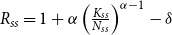 $R_{ss}=1+\alpha \left ( \frac {K_{ss}}{N_{ss}}\right ) ^{\alpha -1}-\delta$
and (B.5), together with
 $\mathbf{F}\big( \theta _{ss}^{\ast }\big) =1-\left ( \frac {\theta _{L}}{\theta _{ss}^{\ast }}\right ) ^{v}$
and
 $ \int _{\theta \leq \theta _{ss}^{\ast }}\left ( \frac {\theta }{\theta _{ss}^{\ast }}\right ) ^{\frac {1}{\sigma }}d\mathbf{F}( \theta ) = \frac {v\sigma }{1-v\sigma }\left [ \left ( \frac {\theta _{L}}{\theta _{ss}^{\ast }}\right ) ^{v}-\left ( \frac {\theta _{L}}{\theta _{ss}^{\ast }} \right ) ^{\frac {1}{\sigma }}\right ]$
, we obtain
 \begin{equation} R_{ss}=1+\frac {\alpha +g-1}{1-g}\delta +\frac {\alpha \Phi }{1-g}\frac {\Gamma \big( \theta _{ss}^{\ast }\big) }{1-\Gamma \big( \theta _{ss}^{\ast }\big) }. \end{equation}
Plug (B.6), with
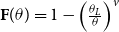 $\mathbf{F}( \theta ) =1-\left ( \frac {\theta _{L}}{\theta }\right ) ^{v}$
and
 $\int _{\theta \gt \theta _{ss}^{\ast }}\theta d \mathbf{F}( \theta ) =\frac {v\left ( \theta _{L}\right ) ^{v}}{v-1} \big( \theta _{ss}^{\ast }\big) ^{1-v}$
, back to (24) to yield (25).
It is clear that the LHS of (25) is decreasing monotonically in
 $ \theta _{ss}^{\ast }$
. In addition, as
 $\theta _{ss}^{\ast }\rightarrow \theta _{L}$
,
 $\frac {1}{v-1}\left ( \frac {\theta _{L}}{\theta _{ss}^{\ast }} \right ) ^{v}$
converges to
 $\frac {1}{v-1}\gt 0$
, given
 $v\gt 1$
. As
 $\theta _{ss}^{\ast }\rightarrow \infty$
,
 $\frac {1}{v-1}\left ( \frac {\theta _{L}}{ \theta _{ss}^{\ast }}\right ) ^{v}$
approaches 0.
Subsequently, we examine the relationship between the RHS of (25) and
 $ \theta _{ss}^{\ast }$
. Note that
 $\Gamma \big( \theta _{ss}^{\ast }\big)$
can re-expressed as
 $\frac {1}{1-v\sigma }\left ( \frac {\theta _{L}}{\theta _{ss}^{\ast }}\right ) ^{\frac {1}{\sigma }}\left [ \left ( \frac {\theta _{L}}{ \theta _{ss}^{\ast }}\right ) ^{v-\frac {1}{\sigma }}-v\sigma \right ]$
. Since
 $\sigma \geq 1$
and
 $v\gt 1$
, it follows that
 $v\sigma \gt \sigma \geq 1$
. Therefore, we have: (1)
 $v\sigma \gt 1$
, (2)
 $v-\frac {1}{\sigma }\gt 0$
, and (3)
 $ 1-v\sigma \lt 0$
. Since
 $\theta _{ss}^{\ast }\gt$
 $\theta _{L}$
, it must be the case that
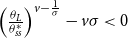 $\left ( \frac {\theta _{L}}{\theta _{ss}^{\ast }}\right ) ^{v-\frac {1 }{\sigma }}-v\sigma \lt 0$
. With
 $\frac {1}{1-v\sigma }\lt 0$
, we conclude that
 $ \Gamma \big( \theta _{ss}^{\ast }\big) \gt 0$
, provided that
 $\sigma \geq 1$
.
Taking the derivative of
 $\Gamma \big( \theta _{ss}^{\ast }\big)$
with respect to
 $\theta _{ss}^{\ast }$
gives
 \begin{equation*} \frac {\partial \Gamma }{\partial \theta _{ss}^{\ast }}=\frac {-v}{1-v\sigma } \left ( \frac {\theta _{L}}{\theta _{ss}^{\ast }}\right ) ^{v}\frac {1}{\theta _{ss}^{\ast }}+\frac {v}{1-v\sigma }\left ( \frac {\theta _{L}}{\theta _{ss}^{\ast }}\right ) ^{\frac {1}{\sigma }}\frac {1}{\theta _{ss}^{\ast }}. \end{equation*}
Evaluating
 $\frac {\partial \Gamma }{\partial \theta _{ss}^{\ast }}$
at
 $ \sigma \geq 1$
gives
 \begin{equation*} \left . \frac {\partial \Gamma }{\partial \theta _{ss}^{\ast }}\right \vert _{\sigma \geq 1}=\frac {-v}{1-v\sigma }\left ( \frac {\theta _{L}}{\theta _{ss}^{\ast }}\right ) ^{v}\frac {1}{\theta _{ss}^{\ast }}\left [ 1-\left ( \frac {\theta _{L}}{\theta _{ss}^{\ast }}\right ) ^{\frac {1}{\sigma }-v}\right ] \lt 0, \end{equation*}
where the inequality comes from
 $v\gt 1$
and
 $\theta _{L}\lt \theta _{ss}^{\ast }$
. As a result, the RHS of (25) is increasing monotonically in
 $\theta _{ss}^{\ast }$
.
Moreover, as
 $\theta _{ss}^{\ast }\rightarrow \theta _{L}$
, we find that
 $ \Gamma \big( \theta _{ss}^{\ast }\big)$
converges to 1 leading the RHS of (25) to approach
 $\frac {1}{\beta }\frac {1-g}{\left ( 1-g\right ) ( 1-\delta ) +\alpha \left ( \delta +\Phi \right ) }-1$
. Given by the condition
 $\frac {1}{\beta }\frac {1-g}{\left ( 1-g\right ) ( 1-\delta ) +\alpha \left ( \delta +\Phi \right ) }-1\lt \frac {1}{v-1}$
, the LHS of ( 25) exceeds the RHS of (25), as
 $\theta _{ss}^{\ast }\rightarrow \theta _{L}$
.
Finally, since the LHS of (25) decreases monotonically in
 $\theta _{ss}^{\ast }$
, and that the RHS of (25) increases monotonically in
 $ \theta _{ss}^{\ast }$
, a unique steady-state cutoff
 $\theta _{ss}^{\ast }$
is established by the intersection of these two expressions.
C. Proof of Proposition3
We begin by taking the derivative of
 $\bar {\Phi }$
with respect to
 $p$
and derive
 \begin{equation} \frac {\partial \bar {\Phi }}{\partial p}=2\frac {p- ( 1-p) \frac {\tau _{ss}}{f}}{\frac {\tau _{ss}}{f+\tau _{ss}}}\lt 0, \end{equation}
where the inequality comes from
 $\frac { ( 1-p) \tau _{ss}}{f}\gt p$
. Given
 $1\gt g$
and
 $\frac {\partial \bar {\Gamma }}{\partial \theta _{ss}^{\ast }} \lt 0$
, a reduction in
 $\bar {\Phi }$
caused by a rise in
 $p$
shifts up the RHS in (25). Thus, to restore the equilibrium, the cutoff
 $\theta _{ss}^{\ast }$
has to fall.
Next, we compute the derivative of
 $\bar {\Phi }$
with respect to
 $f$
:
 \begin{equation} \frac {\partial \bar {\Phi }}{\partial f}=\frac {f^{2}p^{2}- ( 1-p) ^{2}\tau _{ss}^{2}}{\tau _{ss}f^{2}}\lt 0, \end{equation}
where the inequality is due to
 $\frac { ( 1-p) \tau _{ss}}{f}\gt p$
. Given
 $1\gt g$
and
 $\frac {\partial \bar {\Gamma }}{\partial \theta _{ss}^{\ast }} \lt 0$
, an increase in
 $f$
, ceteris paribus, shifts the RHS of (25) upwards, resulting in a reduction of
 $\theta _{ss}^{\ast }$
.
Finally, we derive the derivative of
 $\bar {\Phi }$
with respect to
 $\tau _{ss}$
:
 \begin{equation} \frac {\partial \bar {\Phi }}{\partial \tau _{ss}}=\frac { ( 1-p) ^{2}\tau _{ss}^{2}-f^{2}p^{2}}{\tau _{ss}^{2}f}\gt 0, \end{equation}
where the positive sign is due to
 $\frac { ( 1-p) \tau _{ss}}{f}\gt p$
. Given
 $1\gt g$
and
 $\frac {\partial \bar {\Gamma }}{\partial \theta _{ss}^{\ast } }\lt 0$
, a rise in
 $\tau _{ss}$
, ceteris paribus, puts downward pressure on the RHS of (25). As a result, the cutoff
 $\theta _{ss}^{\ast }$
must increase to uphold the equilibrium.
D. Derivation of equation (31)
Firstly, we employ
 $w_{ss}=\left ( 1-\alpha \right ) \left ( \frac {K_{ss}}{ N_{ss}}\right ) ^{\alpha }$
and (B.5), to derive
 \begin{equation} w_{ss}=\left ( 1-\alpha \right ) \left ( \frac {1}{1-g}\right ) ^{\frac {\alpha }{ \alpha -1}}\left [ \delta +\frac {\Phi \Gamma \big( \theta _{ss}^{\ast }\big) }{1-\Gamma \big( \theta _{ss}^{\ast }\big) }\right ] ^{\frac { \alpha }{\alpha -1}}. \end{equation}
Next, plugging (B.6) and (D.1) with
 $\sigma =1$
and
 $\underline {a}=0$
into (A.1) leads to
 \begin{eqnarray*} x_{ss} &=&\theta _{ss}^{\ast }\frac {w_{ss}\left ( 1-\tau _{ss}\right ) }{\beta R_{ss}} \\ &=&\theta _{ss}^{\ast }\frac {\left ( 1-\alpha \right ) \left ( \frac {1}{1-g} \right ) ^{\frac {\alpha }{\alpha -1}}\left [ \delta +\frac {f+\tau _{ss}}{\tau _{ss}}\left [ p^{2}+ ( 1-p) ^{2}\frac {\tau _{ss}}{f}\right ] \frac { \frac {1}{1-v}\left ( \frac {\theta _{L}}{\theta _{ss}^{\ast }}\right ) ^{v}- \frac {v}{1-v}\left ( \frac {\theta _{L}}{\theta _{ss}^{\ast }}\right ) }{1- \frac {1}{1-v}\left ( \frac {\theta _{L}}{\theta _{ss}^{\ast }}\right ) ^{v}+ \frac {v}{1-v}\left ( \frac {\theta _{L}}{\theta _{ss}^{\ast }}\right ) }\right ] ^{\frac {\alpha }{\alpha -1}}\left ( 1-\tau _{ss}\right ) }{\beta \left [ 1+ \frac {\alpha +g-1}{1-g}\delta +\frac {\alpha }{1-g}\frac {f+\tau _{ss}}{\tau _{ss}}\left [ p^{2}+ ( 1-p) ^{2}\frac {\tau _{ss}}{f}\right ] \frac { \frac {1}{1-v}\left ( \frac {\theta _{L}}{\theta _{ss}^{\ast }}\right ) ^{v}- \frac {v}{1-v}\left ( \frac {\theta _{L}}{\theta _{ss}^{\ast }}\right ) }{1- \frac {1}{1-v}\left ( \frac {\theta _{L}}{\theta _{ss}^{\ast }}\right ) ^{v}+ \frac {v}{1-v}\left ( \frac {\theta _{L}}{\theta _{ss}^{\ast }}\right ) }\right ] } \\ &=&\theta _{ss}^{\ast }\frac {\left ( 1-\alpha \right ) \left ( \frac {1}{1-g} \right ) ^{\frac {\alpha }{\alpha -1}}\left [ \delta +\bar {\Phi }\frac {\bar { \Gamma }\big( \theta _{ss}^{\ast }\big) }{1-\bar {\Gamma }\big( \theta _{ss}^{\ast }\big) }\right ] ^{\frac {\alpha }{\alpha -1}}\left ( 1-\tau _{ss}\right ) }{\beta \left [ 1+\frac {\alpha +g-1}{1-g}\delta +\frac {\alpha \bar {\Phi }}{1-g}\frac {\bar {\Gamma }\big( \theta _{ss}^{\ast }\big) }{1- \bar {\Gamma }\big( \theta _{ss}^{\ast }\big) }\right ] }, \end{eqnarray*}
where we utilize
 $\bar {\Gamma }\big( \theta _{ss}^{\ast }\big) =\frac {1}{ 1-v}\left ( \frac {\theta _{L}}{\theta _{ss}^{\ast }}\right ) ^{v}-\frac {v}{1-v} \left ( \frac {\theta _{L}}{\theta _{ss}^{\ast }}\right )$
and
 $\bar {\Phi }= \frac {f+\tau _{ss}}{\tau _{ss}}\left [ p^{2}+ ( 1-p) ^{2}\frac {\tau _{ss}}{f}\right ]$
in the last line.
E. Extensions
To incorporate non-zero borrowing limits and positive government bond issuance, we assume
 $B_{ss}=bK_{ss}^{\alpha }N_{ss}^{1-\alpha }$
and
 $ \underline {a}=\eta x_{ss}$
, where
 $0\leq b\lt 1$
and
 $\eta \lt 1$
. Assuming
 $ \sigma =1$
, we follow a similar fashion to obtain the following proposition:
Proposition 4.
Impose Assumptions
1
and
2
,
 $\sigma =1$
,
 $\underline {a}=\eta x_{ss}$
,
 $ B_{ss}=bK_{ss}^{\alpha }N_{ss}^{1-\alpha }$
, and
 $G_{ss}=gF\left ( K_{ss},N_{ss}\right )$
with
 $g\lt 1$
. The steady-state cutoff,
 $\theta _{ss}^{\ast }$
, satisfies
 \begin{equation} \frac {1}{v-1}\left ( \frac {\theta _{L}}{\theta _{ss}^{\ast }}\right ) ^{v}= \frac {1}{\beta }\left [ 1+\frac {\alpha -1+g+b\bar {\Phi }\frac { ( 1-\eta ) \bar {\Gamma }\big( \theta _{ss}^{\ast }\big) }{1- ( 1-\eta ) \bar {\Gamma }\big( \theta _{ss}^{\ast }\big) }}{1-g-b\bar {\Phi } \frac { ( 1-\eta ) \bar {\Gamma }\big( \theta _{ss}^{\ast }\big) }{ 1- ( 1-\eta ) \bar {\Gamma }\big( \theta _{ss}^{\ast }\big) }} \delta +\alpha \frac {\bar {\Phi }\frac { ( 1-\eta ) \bar {\Gamma } \big( \theta _{ss}^{\ast }\big) }{1- ( 1-\eta ) \bar {\Gamma } \big( \theta _{ss}^{\ast }\big) }}{1-g-b\bar {\Phi }\frac { ( 1-\eta ) \bar {\Gamma }\big( \theta _{ss}^{\ast }\big) }{1- ( 1-\eta ) \bar {\Gamma }\big( \theta _{ss}^{\ast }\big) }}\right ] ^{-1}-1. \end{equation}
At steady state, as more government bonds are issued or individuals’ borrowing constraints become looser, the steady-state cutoff rises, i.e.,
 $ \frac {\partial \theta _{ss}^{\ast }}{\partial b}\gt 0$
and
 $\frac {\partial \theta _{ss}^{\ast }}{\partial \eta }\lt 0$
In addition, the results,
 $\frac { \partial \theta _{ss}^{\ast }}{\partial p}\lt 0$
,
 $\frac {\partial \theta _{ss}^{\ast }}{\partial f}\lt 0$
, and
 $\frac {\partial \theta _{ss}^{\ast }}{ \partial \tau _{ss}}\gt 0$
, still hold.
Proof. Consider
 $\sigma =1$
,
 $\underline {a}=\eta x_{ss}$
,
 $B_{ss}=bK_{ss}^{\alpha }N_{ss}^{1-\alpha }$
, and
 $G_{ss}=gF\left ( K_{ss},N_{ss}\right )$
. Inserting
 $\int _{\theta \leq \theta _{ss}^{\ast }}\left ( \frac {\theta }{\theta _{ss}^{\ast }}\right ) d\mathbf{F}( \theta ) =\frac {v}{1-v}\left [ \left ( \frac {\theta _{L}}{\theta _{ss}^{\ast }}\right ) ^{v}-\left ( \frac { \theta _{L}}{\theta _{ss}^{\ast }}\right ) \right ]$
and
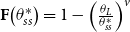 $\mathbf{F}\big( \theta _{ss}^{\ast }\big) =1-\left ( \frac {\theta _{L}}{\theta _{ss}^{\ast } }\right ) ^{v}$
into (17), (22), and (23) gives
 \begin{equation} \frac {C_{ss}}{x_{ss}}=\frac {p^{2}+\frac {\tau _{ss} ( 1-p) ^{2}}{f} }{\frac {\tau _{ss}}{f+\tau _{ss}}} ( 1-\eta ) \left [ \frac {1}{1-v} \left ( \frac {\theta _{L}}{\theta _{ss}^{\ast }}\right ) ^{v}-\frac {v}{1-v} \left ( \frac {\theta _{L}}{\theta _{ss}^{\ast }}\right ) \right ] , \end{equation}
 \begin{equation} \frac {K_{ss}}{x_{ss}}\left ( 1+b\left ( \frac {K_{ss}}{N_{ss}}\right ) ^{\alpha -1}\right ) =1- ( 1-\eta ) \left [ \frac {1}{1-v}\left ( \frac {\theta _{L}}{\theta _{ss}^{\ast }}\right ) ^{v}-\frac {v}{1-v}\left ( \frac {\theta _{L} }{\theta _{ss}^{\ast }}\right ) \right ] . \end{equation}
Dividing
 $\frac {C_{ss}}{x_{ss}}$
in (E.2) by
 $\frac {K_{ss}}{x_{ss}}$
in (E.3) leads to
 \begin{equation} \frac {C_{ss}}{K_{ss}}=\left ( 1+b\left ( \frac {K_{ss}}{N_{ss}}\right ) ^{\alpha -1}\right ) \frac {\frac {p^{2}+\frac {\tau _{ss} ( 1-p) ^{2}}{f}}{ \frac {\tau _{ss}}{f+\tau _{ss}}} ( 1-\eta ) \left [ \frac {1}{1-v} \left ( \frac {\theta _{L}}{\theta _{ss}^{\ast }}\right ) ^{v}-\frac {v}{1-v} \left ( \frac {\theta _{L}}{\theta _{ss}^{\ast }}\right ) \right ] }{1- ( 1-\eta ) \left [ \frac {1}{1-v}\left ( \frac {\theta _{L}}{\theta _{ss}^{\ast }}\right ) ^{v}-\frac {v}{1-v}\left ( \frac {\theta _{L}}{\theta _{ss}^{\ast }}\right ) \right ] }. \end{equation}
Utilizing the resource constraint at steady state gives
 $\left ( 1-g\right ) \left ( \frac {K_{ss}}{N_{ss}}\right ) ^{\alpha -1}=\delta +\frac {C_{ss}}{K_{ss} }$
. Plugging
 $\frac {C_{ss}}{K_{ss}}$
displayed in (E.4) into
 $ \left ( 1-g\right ) \left ( \frac {K_{ss}}{N_{ss}}\right ) ^{\alpha -1}=\delta + \frac {C_{ss}}{K_{ss}}$
, we obtain
 \begin{equation} \left ( 1-g\right ) \!\left ( \frac {K_{ss}}{N_{ss}}\right ) ^{\alpha -1}\!=\delta +\left ( \!1+b\left ( \frac {K_{ss}}{N_{ss}}\right ) ^{\alpha -1}\right ) \frac { p^{2}+\frac {\tau _{ss} ( 1-p) ^{2}}{f}}{\frac {\tau _{ss}}{f+\tau _{ss}}}\frac { ( 1-\eta ) \left [ \!\frac {1}{1-v}\left ( \frac {\theta _{L}}{\theta _{ss}^{\ast }}\right ) ^{v}-\frac {v}{1-v}\left ( \frac {\theta _{L} }{\theta _{ss}^{\ast }}\right ) \!\right ] }{1- ( 1-\eta ) \left [ \!\frac {1}{1-v}\left ( \frac {\theta _{L}}{\theta _{ss}^{\ast }}\right ) ^{v}- \frac {v}{1-v}\left ( \frac {\theta _{L}}{\theta _{ss}^{\ast }}\right ) \!\right ] } . \end{equation}
From (E.5), we solve for
 $\frac {K_{ss}}{N_{ss}}$
:
 \begin{equation} \frac {K_{ss}}{N_{ss}}=\left ( \frac {\delta +\bar {\Phi }\frac { ( 1-\eta ) \bar {\Gamma }\big( \theta _{ss}^{\ast }\big) }{1- ( 1-\eta ) \bar {\Gamma }\big( \theta _{ss}^{\ast }\big) }}{1-g-b\bar {\Phi } \frac { ( 1-\eta ) \bar {\Gamma }\big( \theta _{ss}^{\ast }\big) }{ 1- ( 1-\eta ) \bar {\Gamma }\big( \theta _{ss}^{\ast }\big) }} \right ) ^{\frac {1}{\alpha -1}}. \end{equation}
Substituting
 $\frac {K_{ss}}{N_{ss}}$
into firm’s profit-maximizing conditions yields
 \begin{eqnarray*} R_{ss} &=&1+\alpha \left ( \frac {K_{ss}}{N_{ss}}\right ) ^{\alpha -1}-\delta \\ &=&1+\frac {\alpha -1+g+b\bar {\Phi }\frac { ( 1-\eta ) \bar {\Gamma } \big( \theta _{ss}^{\ast }\big) }{1- ( 1-\eta ) \bar {\Gamma } \big( \theta _{ss}^{\ast }\big) }}{1-g-b\bar {\Phi }\frac { ( 1-\eta ) \bar {\Gamma }\big( \theta _{ss}^{\ast }\big) }{1- ( 1-\eta ) \bar {\Gamma }\big( \theta _{ss}^{\ast }\big) }}\delta +\alpha \frac {\bar {\Phi }\frac { ( 1-\eta ) \bar {\Gamma }\big( \theta _{ss}^{\ast }\big) }{1- ( 1-\eta ) \bar {\Gamma }\big( \theta _{ss}^{\ast }\big) }}{1-g-b\bar {\Phi }\frac { ( 1-\eta ) \bar { \Gamma }\big( \theta _{ss}^{\ast }\big) }{1- ( 1-\eta ) \bar { \Gamma }\big( \theta _{ss}^{\ast }\big) }}, \end{eqnarray*}
where we employ (E.6).
By exploiting the Euler equation (14), we derive
 $\frac {1}{\beta R_{ss}}=1+ \frac {1}{v-1}\left ( \frac {\theta _{L}}{\theta _{ss}^{\ast }}\right ) ^{v}$
. Inserting
 $R_{ss}$
in (E.7) back to
 $\frac {1}{\beta R_{ss}}=1+\frac {1 }{v-1}\left ( \frac {\theta _{L}}{\theta _{ss}^{\ast }}\right ) ^{v}$
results in (E.1) which pins down the steady-state cutoff
 $\theta _{ss}^{\ast }$
.
Clearly, the LHS in (E.1) decreases in
 $\theta _{ss}^{\ast }$
. In addition, given
 $\frac {\partial \bar {\Gamma }}{\partial \theta _{ss}^{\ast }}\lt 0$
, the RHS in (E.1) increases in
 $\theta _{ss}^{\ast }$
. It can be seen from (E.1) that a rise in
 $b$
shifts the RHS downwards, leading to a greater
 $\theta _{ss}^{\ast }$
. Whereas, a higher
 $ \eta$
puts upward pressure on the RHS, thus reducing
 $\theta _{ss}^{\ast }$
. In addition, an increase in
 $ \bar {\Phi }$
, triggered by a decline in either
 $p$
or
 $f$
, or a rise in
 $\tau _{ss}$
, exerts downward pressure on the RHS in (E.1). As a result, the results,
 $ \frac {\partial \theta _{ss}^{\ast }}{\partial p}\lt 0$
,
 $ \frac {\partial \theta _{ss}^{\ast }}{\partial f}\lt 0$
, and
 $ \frac {\partial \theta _{ss}^{\ast }}{\partial \tau _{ss}}\gt 0$
, still hold.
As illustrated in Proposition4, fewer individuals encounter binding borrowing limits when the government increases its issuance of bonds at steady state. This result is reminiscent of the findings in the works by Chien and Wen (Reference Chien and Wen2022) and Chen et al. (Reference Chen, Chien, Wen and Yang2021). An immediate policy implication is that an increased issuance of government bonds helps relax individuals’ borrowing constraints. Furthermore, another result highlighted in Proposition4 indicates that the proportion of financially constrained individuals rises with the stringency of borrowing limits. More importantly, the results in Proposition C remain robust, given
 $0\leq b\lt 1$
and
 $\eta \lt 1$
.