3.1 Speed of the head

One of the key properties of a gravity current is the speed of the head of the current, $\text{d}x_{n}/\text{d}t$ . From dimensional analysis, we expect this to scale with $B_{o}^{1/3}$ , although, as seen in figure 4(a), there is also a weak dependence on $Fr_{o}$ ,

(3.1) $$\begin{eqnarray}\frac{\text{d}x_{n}}{\text{d}t}=\unicode[STIX]{x1D706}(Fr_{o})B_{0}^{1/3},\end{eqnarray}$$

where $\unicode[STIX]{x1D706}$ may be approximated by the relation (figure 4 b)

(3.2a,b ) $$\begin{eqnarray}\unicode[STIX]{x1D706}=0.85+0.17Fr_{o}\quad \text{for }Fr_{0}<1\quad \text{and}\quad \unicode[STIX]{x1D706}=1.1\pm 0.1\quad \text{for }Fr_{0}>1.0.\end{eqnarray}$$

We also measured the vertical integral of the buoyancy, $\overline{g^{\prime }h}_{n}$ , just behind the head of the flow, at the point where $h$ has its maximum, $h_{n}$ . The ratio of the speed of the nose, $\text{d}x_{n}/\text{d}t$ , and $(\overline{g^{\prime }h}_{n})^{1/2}$ yields an estimate for the Froude number of the front of the current, $Fr_{n}$ . Figure 4(c) shows that $Fr_{n}\approx 1.1\pm 0.05$ for $0.1<Fr_{o}<3.7$ .

Figure 4.

Experiments A–K. (a) Position of the dimensionless head of the current, $x_{n}(t)/h_{o}$ , as a function of dimensionless time, $tB_{o}^{1/3}/h$ , for each of the experiments. The symbols for the different experiments are A, black empty circles; B, green solid triangles; C, green empty triangles; D, black empty squares; E, orange pluses; F, red empty circles; G, red solid circles; H, light blue stars; I, pink crosses; J, black solid squares; K, blue empty diamonds. (b) Variation of the constant $\unicode[STIX]{x1D706}$ as a function of the source Froude number (3.2). (c) Variation of the Froude number of the head, $Fr_{n}$ , as a function of the source Froude number, $Fr_{o}$ .

Figure 5.

Photograph of the current just downstream of the source, in the region $0<x<30h_{o}$ , for the cases (a) $Fr_{o}=2.7$ and (b) $Fr_{o}=0.4$ . In (a), the current develops a turbulent mixing zone in the region $0<x<20h_{o}$ , reminiscent of an extended hydraulic jump or jet mixing zone, while further downstream the flow depth is more uniform and there is little indication of further turbulent mixing on the upper surface of the current. In (b), the flow initially accelerates and plunges on entering the tank, and this is then followed by a turbulent mixing region in which the current slowly deepens over a distance of order $5h_{o}$ . In both cases, downstream of the mixing zone, there is a region of near constant depth. The velocity profiles are measured at the point labelled with the vertical dashed line.

Figure 6.

(a–c) Variation of the vertical profile of salt concentration normalised by the source salt concentration as measured just downstream of the inflow mixing zone (solid line) and at a distance $0.1x_{n}$ behind the head of the flow (dotted line), and the horizontal speed, normalised by the maximum horizontal speed just downstream of the inflow mixing zone (triangles, dashed line) as a function of normalised height. The height is normalised relative to the total depth of the current at this point. Curves are shown for three source Froude numbers (experiments B3, G3 and J3), illustrating the different profiles of the source current immediately downstream of the mixing region for the cases of small, moderate and substantial mixing in the inflow mixing zone. (d) Estimate of the gradient Richardson number in the current just downstream of the inflow mixing zone as a function of the source Froude number.

3.2 Mixing near the inflow

Once the incoming jet of saline water entered the base of the tank, a local zone of flow adjustment and mixing developed. This region extended a distance of order 30–70 cm into the tank, increasing with the source Froude number. Beyond this zone, the current depth evolved much more slowly with distance down the tank. Examples of the inflow adjustment are shown in figure 5 for the cases (a) $Fr_{o}=2.7$ and (b) $Fr_{o}=0.4$ . In the case $Fr_{o}=2.7$ , the current deepens over a distance of approximately 70 cm, with a significant amount of turbulent mixing apparent on the upper surface of the flow. Further downstream, the depth then evolves more gradually. In the case $Fr_{o}=0.4$ , the current initially accelerates and thins out, but then it appears to deepen and mix across its upper surface as in the case of the larger source Froude number. Again, it reaches a near constant depth at a distance of approximately $5h_{o}$ , after which it evolves much more slowly downstream.

The flux of ambient fluid entrained in this mixing zone could be found by measuring the vertical profile of the horizontal velocity just downstream of the mixing zone and comparing this with the source volume flux. The vertical profile of the horizontal velocity was found by tracking the motion of a series of vertical lines of dye released into the flow. The lateral extent of the mixing zone was found by determining the point at which the current depth tended to a more uniform value with position, and the vertical lines of dye were then released downstream of this point. Since the entrainment per unit distance downstream of the inflow mixing zone appeared to be small compared with the mixing in this initial adjustment region (see below), our measurement of the flow was insensitive to the precise location of the point at which we released the dye, provided that this was downstream of but close to the inflow mixing zone. In all cases, the dye was released within a distance of 10–20 cm downstream of the inflow mixing zone, a small distance relative to the 5 m long flume. As the current advanced downstream, our measurements suggest that the volume flux mixed into this near-source region remained approximately constant.

In figure 6, we present the normalised vertical profile of the horizontal velocity, $\hat{u}$ , where $\hat{u} =u/u_{max}$ , with $u_{max}$ the maximum value of $u$ at this position (dashed line). We also present the normalised concentration, ${\hat{c}}$ , where ${\hat{c}}=c/c_{o}$ , with $c_{o}$ the concentration of salt in the source fluid, as a function of normalised height, ${\hat{h}}$ , where ${\hat{h}}=h/h_{max}$ , with $h_{max}$ the maximum value of $h$ at this position (solid line). The maximum value of $h$ corresponds to the point at which the concentration falls below the fraction 0.05 of the original source fluid. For reference, we also present the concentration of salt in the head of the current, as measured a distance $0.1x_{n}$ behind the actual front of the flow, $x_{n}(t)$ (dotted line). In figure 6, profiles are shown for three source Froude numbers, $Fr_{o}=0.4$ , 1.5 and 2.7. We integrated the velocity profile to estimate the volume flux, per unit width, in the current downstream of the adjustment zone, $Q_{m}$ . This was used to estimate the flux of ambient fluid, per unit width, that was mixed into the current in this transition zone, $Q_{m}-Q_{o}$ , and the ratio $e_{in}=Q_{m}/Q_{o}-1$ is shown in figure 7(a) (solid circles). As a check on the accuracy of this measurement, we estimated the buoyancy flux in the current at this point by integrating the product of the velocity and buoyancy over the height of the current. We found that in all experiments this was within 10 % of the source buoyancy flux, per unit width. The data in figure 7(a) show that for low $Fr_{o}$ , there is relatively little mixing in the inflow mixing zone and $e_{in}=0.2\pm 0.1$ . In this case, the current has a relatively uniform density and velocity with height up to the point at which there is a transition to the overlying ambient fluid (figure 6 a). As $Fr_{o}$ increases, there is more entrainment near the source (figure 7 a), with $e_{in}$ increasing to values of order $0.7\pm 0.1$ when $Fr_{o}=3.7$ . In this case, at points downstream of the inflow mixing zone, the current density and velocity vary continuously over the full depth of the current (figure 6 b,c).

As noted above, in the case that $Fr_{o}>1$ , then on inflow the flow is supercritical and begins to mix and deepen after entering the tank (figure 5 a). In contrast, with $Fr_{o}<1$ , the inflow is subcritical, but on entering the tank, the flow accelerates and thins to become supercritical some distance beyond the inflow (figure 5 b), and then it appears to mix and deepen. Our data reveal that just beyond the inflow mixing zone, the flow has become stratified in velocity and buoyancy, with the lowest part of the flow being of nearly constant speed and density, and the upper part of the flow having a vertical gradient in velocity and buoyancy, below the ambient fluid. The stability of such a region depends on the gradient Richardson number, $Ri_{g}=\text{d}g^{\prime }/\text{d}z/(\text{d}u/\text{d}z)^{2}$ , with the flow being stable for $Ri_{g}>0.25$ (Turner Reference Turner1979). If we approximate the density and velocity profiles measured in the current just downstream of the inflow mixing zone (e.g. figure 6) as having an upper region that is linearly stratified in density and velocity and a lower region of constant speed and buoyancy, then we estimate that the gradient Richardson number has a value that increases from $0.4\pm 0.15$ when $Fr_{o}=3.7$ to $1.15\pm 0.15$ as $Fr_{o}$ decreases to a value of $0.7$ , as shown in figure 6(d). This suggests that downstream of the inflow mixing zone, the current has become stable.

Figure 7.

(a) Variation of the total fractional mixing in the current, $(\text{d}V/\text{d}t)/Q_{o}-1$ (solid triangles), the fractional mixing in the inflow region, $e_{in}=Qm/Q_{o}-1$ (solid circles), and the fractional mixing in the remainder of the current, $e_{n}$ ((3.3); open circles), as a function of the source Froude number. (b) Total volume of the current per unit width as a function of time. The symbols for the different experiments are A, black empty circles; B, green solid triangles; C, green empty triangles; D, black empty squares; E, orange pluses; F, red empty circles; G, red solid circles; H, light blue stars; I, pink crosses; J, black solid squares; K, blue empty diamonds. (c) Variation of the nose entrainment parameter, $E$ , as defined by (3.5), representing the fraction of the fluid initially ahead of the current which is entrained by the current as it is displaced over the head of the current.

3.3 Mixing near the head

We also measured the rate of increase of the total volume of the current, per unit width, as a function of time by calculating the area of the region in which the concentration of dye is in excess of a threshold value, which we set to be equal to 0.05 of the initial concentration of the source fluid (figure 7 b). We varied the threshold value used to measure the total volume and we estimate the error in our measurements to be less than 5 % (cf. Sher & Woods Reference Sher and Woods2015). We find that to good approximation, $V(t)$ , the volume per unit width, increases linearly with time as the current advances downstream, as shown in figure 7(b) for each of the experiments (A–K, table 1). 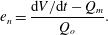The rate of increase of $V(t)$ with time does not depend strongly on $Fr_{o}$ , and values in the range $1.8Q_{0}<\text{d}V/\text{d}t<2.1Q_{0}$ are shown in figure 7(a) with solid triangles. This suggests that overall the current fluid is diluted to an average concentration of approximately 0.4–0.55 of the source fluid. If we compare the rate of volume increase in the whole current with the measured volume flux per unit width downstream of the near-source mixing zone, $Q_{m}$ , we can estimate the rate of entrainment of fluid in the remainder of the flow as a fraction of the source volume flux,

(3.3) $$\begin{eqnarray}e_{n}=\frac{\text{d}V/\text{d}t-Q_{m}}{Q_{o}}.\end{eqnarray}$$

The results of this calculation are shown in figure 7(a) (open circles), and illustrate the shifting balance between mixing near the source for large source Froude number and mixing downstream for smaller source Froude number.

If we follow the classical parameterisation for the rate of entrainment of ambient fluid into the upper surface of the flow and take it to be of the form $\unicode[STIX]{x1D6FC}(Fr(x,t))u(x,t)$ per unit area, where $Fr$ is a local Froude number for the flow (Ellison & Turner Reference Ellison and Turner1959; Dallimore, Imberger & Ishikawa Reference Dallimore, Imberger and Ishikawa2001; Chowdhury & Testik Reference Chowdhury and Testik2015), then we would expect the total volume of the current per unit width to increase according to the relation

(3.4) $$\begin{eqnarray}\frac{\text{d}V}{\text{d}t}=Q_{o}+e_{in}Q_{o}+\int _{L_{o}}^{L(t)-L_{n}}\unicode[STIX]{x1D6FC}(Fr(x,t))u\,\text{d}x+e_{h}Q_{o},\end{eqnarray}$$

where $e_{h}$ is the fraction of the mixing that occurs at the head of the flow, in a region of length $L_{n}$ , say, just behind the head, estimated to be of order 3– $5h_{n}$ , and $L_{o}$ is the length of the mixing zone near the inflow, estimated to be of order 5– $15h_{n}$ . The middle term on the right-hand side then represents the entrainment along the upper boundary of the main part of the current away from the inflow adjustment zone and the head. If this entrainment was significant in our experiments, we would expect a gradual increase in the rate of change of volume with time, since $u$ is nearly constant and $L(t)$ increases linearly with time (cf. Johnson & Hogg Reference Johnson and Hogg2013). However, our experimental data show that, to good approximation, the volume increases at a rate proportional to $t$ (figure 7 b). We infer that, for the length scale of the currents explored in this study, which travel 5 m along the flume, corresponding to a distance of order $L(t)\leqslant (50{-}100)h_{n}$ , any mixing on the upper surface of the flow is small compared with the sum of the mixing at the source and the nose of the flow, and so $e_{h}\simeq e_{n}$ .

This interpretation is consistent with our dye experiments (figure 3 b,d), since there is little evidence of vigorous mixing of ambient fluid into the current in the region between the inflow mixing zone and the nose of the flow; indeed, the interfaces that demarcate changes in dye colour appear to remain sharp as they stretch in the direction of flow over time (figure 3). Moreover, the billows and other mixing structures on the upper surface of the flow appear to be much weaker upstream of the near-head mixing zone. In figure 3, we have compared the speed of the relatively dense fluid lower in the current with the speed of the head of the current: in the case of a small source $Fr_{o}$ , more ambient fluid is mixed into the head, and so the relatively dense fluid in the current takes longer to reach the front of the flow than in the case of larger $Fr_{o}$ , where less ambient is mixed into the head. This is manifested by a larger difference in speed of the fluid at the base of the current relative to the speed of the head for larger $Fr_{o}$ , as seen in figure 3.

Figure 8.

The evolution with dimensionless time ( $y$ -axis) of contours of (a–c) the fraction of the total volume and (d–f) the fraction of the total buoyancy of the current, in the region $0<\unicode[STIX]{x1D709}<\unicode[STIX]{x1D702}$ , as a function of $\unicode[STIX]{x1D702}$ ( $x$ -axis) for $0<\unicode[STIX]{x1D702}<1$ . Time is scaled relative to the time to travel a distance equal to the depth of the head of the current. The contours correspond to the values $0.1,0.2,\ldots ,1.0$ . (g–i) Concentration field throughout the current at one instant in time. The image is shown in false colour, with the concentration being given by the scale bar ( $\text{g}~\text{kg}^{-1}$ ). Measurements are shown for three gravity currents, corresponding to (a,d,g) $Fr_{o}=0.4$ (experiment B), (b,e,h) $Fr_{o}=1.5$ (experiment G) and (c,f,i) $Fr_{o}=2.7$ (experiment J).

The quantity $e_{n}$ (3.3) can be represented in terms of the fraction of the fluid displaced by the head of the gravity current that is mixed into the current, $E$ , according to the balance (Sher & Woods Reference Sher and Woods2015)

(3.5) $$\begin{eqnarray}Eh_{n}\frac{\text{d}x_{n}}{\text{d}t}=e_{n}Q_{o}.\end{eqnarray}$$

The variation of $E$ with $Fr_{0}$ is shown in figure 7(c). Currents for which $Fr_{0}<1$ involve relatively little mixing near the inflow but have a much larger entrainment at the head of the flow, with $E$ decreasing from $0.4\pm 0.08$ to $0.1\pm 0.08$ as $Fr_{0}$ increases from 0.4 to 3.7. We note that Sher & Woods (Reference Sher and Woods2015) found that in the different case of a finite-release gravity current, once the flow becomes self-similar, $E$ has a value in the range 0.6–0.75. For the present experiments, figure 6(d) illustrates that downstream of the initial mixing zone, the gradient Richardson number in the currents becomes progressively larger as $Fr_{o}$ decreases; this increasing stability of the flow may be related to the greater mixing in the head of the flow, since we also find that $E$ increases as $Fr_{o}$ decreases. It would be interesting to measure the gradient Richardson number in a finite-release current to establish whether this is also consistent with the greater value of $E$ in such currents.

3.4 Self-similarity

Given that our data suggest that the mixing occurs primarily near the inflow and the head of the flow, and that the speed of the flow is nearly constant, we might anticipate that the currents take on a long-time asymptotic self-similar structure in which the distribution of density and volume along the current is primarily a function of the position relative to the nose, $\unicode[STIX]{x1D702}=x/x_{n}(t)$ . Further, we might anticipate that this structure depends on the source Froude number given the different partitioning of the mixing between the inflow and the head and the different vertical structure of the flow. To explore this hypothesis, in figure 8, we show the evolution with dimensionless time (vertical axis) of contours of (a–c) the fraction of the total volume and (d–f) the fraction of the total buoyancy of the current, in the region $0<\unicode[STIX]{x1D709}<\unicode[STIX]{x1D702}$ , as a function of $\unicode[STIX]{x1D702}$ (horizontal axis) for $0<\unicode[STIX]{x1D702}<1$ . Time is scaled relative to the time to travel a distance equal to the depth of the head of the current. The contours of fractional volume and fractional buoyancy correspond to the values $0.1,0.2,\ldots ,1.0$ . Measurements are shown for three gravity currents, with input Froude numbers of 0.4 (a,d), 1.5 (b,e) and 2.7 (c,f). In each case, there is an initial transition period as the current becomes established after which the contours become nearly independent of time, and the structure of the current then appears to depend primarily on $\unicode[STIX]{x1D702}$ and $Fr_{o}$ . It would be interesting to explore how the currents evolve over even greater distances from the source.

For each of the currents in figure 8, in (g–i), we illustrate the concentration field throughout the current at one instant in time. In (g), with $Fr_{0}<1$ , there is less mixing in the inflow adjustment region (figure 7 a). A relatively dense region of fluid at the base of the flow then advances towards the head of the flow (figure 3 d). Here, it rises and mixes with the displaced ambient fluid, forming the upper wake region of relatively low density which extends backwards from the nose of the current (figure 8 a,d,g). Given the large amount of mixing near the head, the low-density region near the nose occupies a relatively large fraction of the depth of the current; however, as the current continues forward, and new source fluid migrates along the base of the tank, this upper mixed wake region shears out behind the head and hence occupies a progressively smaller fraction of the depth of the flow. In contrast, with higher inlet Froude numbers, there is much more mixing of ambient fluid in the near-source mixing zone (figures 3 a,b; 5 a). This leads to a much more continuous vertical stratification (figure 6 c) and there is less mixing of the displaced ambient fluid into the head of the flow (figure 7 a, figure 8).