1. Introduction
The phenomenon of undulating waves developing on a liquid thread and leading to breakup of the thread is ubiquitous in nature (Challita, Rohilla & Saad Bhamla Reference Challita, Rohilla and Bhamla2024) and engineering applications (e.g. inkjet printing (Lohse Reference Lohse2021), drug encapsulation and delivery (Loscertales et al. Reference Loscertales, Barrero, Guerrero, Cortijo, Marquez and Gañán-Calvo2002; Arora et al. Reference Arora, Hakim, Baxter, Rathnasingham, Srinivasan, Fletcher and Mitragotri2007)). The process is mainly driven by surface tension and is known as a Rayleigh–Plateau (RP) instability problem (Lord Reference Lord1878, Reference Lord1892). It has been the subject of extensive investigation and is now well understood (Eggers Reference Eggers1997; Eggers & Villermaux Reference Eggers and Villermaux2008). With the fast development of nanoscale technology and the promising application perspective of liquid threads at the nanoscale, many researchers have investigated the instability and breakup problem of nano liquid threads/jets. Early studies (Koplik & Banavar Reference Koplik and Banavar1992; Kawano Reference Kawano1998) using molecular dynamics (MD) simulation concluded that the instability of nano liquid jets can be qualitatively described by Rayleigh’s classic linear stability theory (Lord Reference Lord1878, Reference Lord1892). However, Moseler & Landman (Reference Moseler and Landman2000) noted that the profile shape of nano liquid threads near breakup is very different from that of macroscopic liquid jets. They proposed a one-dimensional stochastic lubrication equation (SLE), which is an extension of Eggers’ lubrication equation (Eggers & Dupont Reference Eggers and Dupont1994) but incorporates the effect of thermal fluctuations using the Landau–Lifshitz–Navier–Stokes equations (Landau & Lifshitz Reference Landau and Lifshitz1980). This SLE has been proved to be very successful in predicting the profile shape of nano liquid threads/jets (Moseler & Landman Reference Moseler and Landman2000). The special breakup mode (symmetric double-cone mode) observed in MD simulations was also successfully explained by the self-similarity analysis of the SLE (Eggers Reference Eggers2002), and was validated by experiments (Hennequin et al. Reference Hennequin, Aarts, Van Der Wiel, Wegdam, Eggers, Lekkerkerker and Bonn2006; Petit et al. Reference Petit, Rivière, Kellay and Delville2012). In recent years, linear stability analysis based on the SLE was conducted by Zhao, Sprittles & Lockerby (Reference Zhao, Sprittles and Lockerby2019) to investigate the RP-like instability of nano liquid threads. The time-dependent capillary wave spectra were obtained from the analysis. It was found that there is a very good agreement between MD simulation results and SLE-RP theory (Zhao et al. Reference Zhao, Sprittles and Lockerby2019; Zhang, Zhao & Si Reference Zhang, Zhao and Si2024), further confirming the validity of SLE. Zhao et al. (Reference Zhao, Sprittles and Lockerby2019) also demonstrated that thermal fluctuations can considerably accelerate the growth of perturbations and cause the critical dimensionless wavenumber to be larger than 1. Subsequently, Zhang et al. (Reference Zhang, Zhao and Si2024) found that the competition between thermal fluctuations and hydrodynamics leads to two distinct regimes with different rupture modes: uniform rupture for the hydrodynamics regime and non-uniform rupture for the thermal-fluctuation regime.
The instability of thin liquid films on solid boundaries is closely related to the instability problem of a liquid thread. They are both two-dimensional problems that have a very small length scale in one dimension compared with the other one. The lubrication approximation is applicable to them. The lubrication equations for planar liquid films on plates and annular liquid films on cylindrical surfaces have been known for many years (Oron, Davis & Bankoff Reference Oron, Davis and Bankoff1997; Kliakhandler, Davis & Bankoff Reference Kliakhandler, Davis and Bankoff2001; Craster & Matar Reference Craster and Matar2006), and have been extended to include thermal fluctuations by Grün et al. (Reference Grün, Mecke and Rauscher2006) and Zhang, Sprittles & Lockerby (Reference Zhang, Sprittles and Lockerby2020), respectively. Linear stability analysis based on these SLEs and MD simulations (Zhang et al. Reference Zhang, Sprittles and Lockerby2019, Reference Zhang, Sprittles and Lockerby2020) both show that thermal fluctuations are capable of accelerating film rupture and cause the dominant wavenumber to evolve with time. The critical dimensionless wavenumber also becomes larger than 1. These effects of thermal fluctuations on nano liquid films are very similar to those on nano liquid threads. Zhang et al. (Reference Zhang, Sprittles and Lockerby2020) further considered the slip effects and revealed that slip also accelerates the growth of instability. These works exemplify the significant influences of nanoscale factors, and the power of stochastic lubrication-type equations to reveal their influence mechanism.
Evaporation and condensation have been reported to considerably change the pinch-off profile of a nano liquid thread (Kang & Landman Reference Kang and Landman2007; Gopan & Sathian Reference Gopan and Sathian2014). This was analysed by Kang & Landman (Reference Kang and Landman2007) through a modified SLE and it was shown that, when the evaporation and condensation process is considered, an additional mass redistribution flux along the thread is caused by the curvature-dependent evaporation. This mass redistribution flux was said to transform the double-cone pinch-off profile to a long-thread profile. Evaporation and condensation can be controlled by the surrounding vapour pressure, and hence may open up a new avenue to actively control the instability and breakup of nano liquid threads/jets. In addition to this potential application, the formation and breakup of liquid bridges, which play an important role in the behaviours of moist granular materials, can be considerably affected by evaporation–condensation (Maeda, Israelachvili & Kohonen Reference Maeda, Israelachvili and Kohonen2003). Therefore, it is of great interest to elucidate how evaporation–condensation will influence the instability and breakup of nano liquid threads/jets. We note that a stability analysis on nano liquid threads taking into account both thermal fluctuations and evaporation–condensation is still lacking in the literature. In this article, we aim to fill this gap and analyse how the evaporation–condensation influences the instability of nano liquid threads.
In § 2 we propose a modified stochastic lubrication equation (MSLE) that is different from that of Kang & Landman (Reference Kang and Landman2007). In §§ 3, 4 we conduct linear stability analysis using this MSLE for a long liquid thread in a saturated or supersaturated vapour environment. In § 5, we analyse the stochastic instability behaviour of a short liquid thread whose length is close to the critical length in Rayleigh’s classic theory. In § 6 we present our MD simulation model. In § 7 we discuss our theoretical results and validate them with MD simulations. We draw conclusions in the last section.
2. Modified stochastic lubrication equation
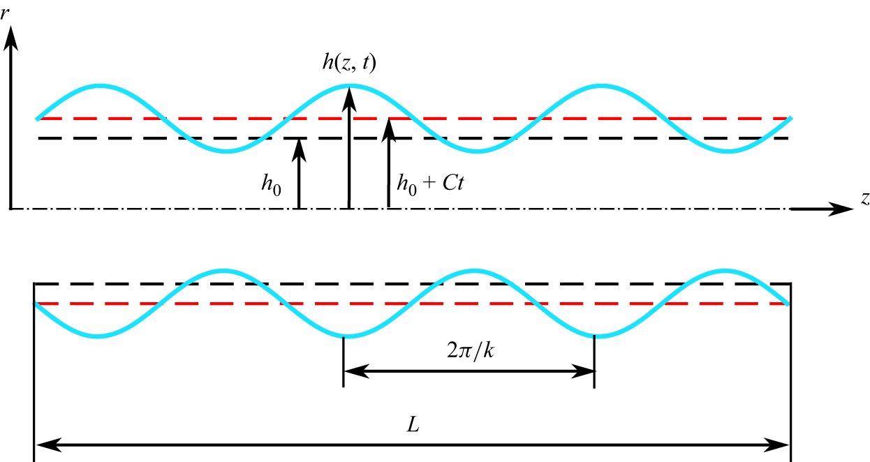
Schematic of the liquid thread instability. Here,
 $z$
is the axial coordinate,
 $r$
is the radial coordinate. The thread is infinitely long but only a portion with length
 $L$
is taken for study. The blue solid line depicts the profile of the liquid thread. The parameter
 $h$
is the radius of the thread as a function of
 $z$
and
 $t$
and
 $k$
is the wavenumber of the perturbation wave. The black dashed line depicts the profile of the cylindrical liquid thread at
 $t=0$
. The value of
 $h_0$
is the radius of this initial cylindrical thread and
 $C$
is a condensation parameter which will be defined below. The red dashed line depicts the time-dependent basic state that we will explain and use in § 4.

We consider an axisymmetric liquid thread in a cylindrical coordinate system, as depicted in figure 1. The initially cylindrical liquid thread has an initial radius
 $h_0$
. The thread is infinitely long but we take only a finite length
 $L$
for study. The SLE (Moseler & Landman Reference Moseler and Landman2000) that describes the evolution of thread profile and axial flow velocity reads
 \begin{equation} \frac {\partial h}{\partial t} = - uh^{\prime} - \frac {u^{\prime}h}{2}, \end{equation}
 \begin{equation} \frac {\partial u}{\partial t} = -u u^{\prime} - \frac {p^{\prime}}{\rho } + 3\nu \frac {(h^2u^{\prime})^{\prime}}{h^2} + \sqrt {\frac {6k_BT\nu }{\rho \pi }}\frac {(h\mathcal{N})^{\prime}}{h^2}, \end{equation}
where
 $h(z,t)$
is the thread radius,
 $u(z,t)$
is the axial flow velocity, both being functions of the axial coordinate
 $z$
and time
 $t$
,
 $p=\gamma \kappa$
is the pressure,
 $\kappa =h^{-1}(1+(h^{\prime})^2)^{-1/2}-h^{\prime\prime}(1+(h^{\prime})^2)^{-3/2}$
is the sum of the principal curvatures,
 $\rho$
is the fluid density,
 $\nu$
is the kinematic viscosity,
 $\gamma$
is the surface tension,
 $T$
is the temperature,
 $k_B$
is the Boltzmann constant,
 $\mathcal{N}$
is white noise with correlation function
 $\langle \mathcal{N}(z,t) \mathcal{N}(z^{\prime},t^{\prime})\rangle = \delta (z-z^{\prime})\delta (t-t^{\prime})$
and
 $\langle \boldsymbol{\cdot }\rangle$
denotes the ensemble average. The prime notation indicates derivative against
 $z$
, except when the prime is on
 $t$
or
 $z$
where it simply means another time or location variable.
Then we consider the evaporation–condensation process. There are two predominant evaporation–condensation models: the diffusion-limited model (Wilson & D’Ambrosio Reference Wilson and D’Ambrosio2023) and the one-sided model (Burelbach, Bankoff & Davis Reference Burelbach, Bankoff and Davis1988; Ajaev Reference Ajaev2005). The diffusion-limited model assumes that the evaporation process is rate limited by the diffusive transport of vapour. The one-sided model assumes that the evaporation process is rate limited by the phase change. Both are widely used and they can produce greatly different predictions (Larsson & Kumar Reference Larsson and Kumar2023). Since we are considering a nano liquid thread in its own vapour, we believe it is more appropriate to use the one-sided model (Cazabat & Guéna Reference Cazabat and Guéna2010; Larson Reference Larson2014). The one-sided model provides a constitutive equation that relates the mass flux at the interface to the local surface temperature (Burelbach et al. Reference Burelbach, Bankoff and Davis1988). It is derived by linearising the Hertz–Knudsen relation (Schrage Reference Schrage1953) using the Clausius–Clapeyron law. But since the system we study here could have a high supersaturation ratio, the linearisation becomes inaccurate. It is necessary to directly adopt the Hertz–Knudsen relation to predict the evaporation–condensation flux.
The vapour pressure at the surface of the liquid thread is given by the Kelvin or Thomson–Gibbs equation (Hinds Reference Hinds1999)
 \begin{equation} P_s = P_0 \exp {\left (\frac {\kappa \gamma V_0}{k_BT}\right)}\approx P_0\left (1+\frac {\kappa \gamma V_0}{k_B T}\right)\!, \end{equation}
where
 $P_0$
is the saturation vapour pressure at a planar surface and
 $V_0$
is the molecular volume in liquid phase. Using the Hertz–Knudsen relation, the local volume flux
 $J_v$
due to evaporation–condensation can be determined
 \begin{equation} J_v = \frac {\alpha _{c} P_0V_0 \left (1+\dfrac {\kappa \gamma V_0}{k_B T}-S\right)}{\sqrt {2\pi mk_B T}}, \end{equation}
where
 $m$
is the molecular weight,
 $S=P_v/P_0$
is the supersaturation ratio of the surrounding vapour,
 $P_v$
is the realistic surrounding vapour pressure and
 $\alpha _c$
is the anomalous evaporation/condensation coefficient;
 $0\lt \alpha _c\lt 1$
, describing the probability of phase change. The exact value of
 $\alpha _c$
is a matter of debate and is usually used to match experimental results to theoretical results. As the evaporation and condensation processes are separately Poisson processes,
 $J_v$
should also be a fluctuating quantity. However, in the following analysis we will neglect the fluctuations in
 $J_v$
. In Appendix A we provide a formal analysis of the influence of these flux fluctuations and show that they are indeed negligible.
To derive the mass conservation equation that accounts for the evaporation–condensation flux we start from the generalised kinematic boundary condition
 \begin{equation} \boldsymbol{n}\boldsymbol{\cdot }(\boldsymbol{v}|_{r=h}-\dot {\boldsymbol{x}})=J_v ,\end{equation}
where
 $\boldsymbol{n}$
is the unit normal vector to the interface,
 $\boldsymbol{v}$
is the fluid velocity and
 $\dot {\boldsymbol{x}}$
is the interface velocity. The unit normal vector is given by
 $\boldsymbol{n}=[1,-h^{\prime}]/\sqrt {1+(h^{\prime})^2}$
. The fluid velocity has two components: a radial component
 $v_r$
and an axial component
 $v_z$
, thus
 $\boldsymbol{v}=[v_r,v_z]$
. The interface velocity is given by
 $\dot {\boldsymbol{x}}=[\partial h/ \partial t,0]$
. After substitution of these parameters into (2.5) we have
 \begin{equation} -\frac {\partial h}{\partial t} + v_r|_{r=h} - v_z|_{r=h} h^{\prime} = J_v\sqrt {1+\left (h^{\prime}\right)^2}. \end{equation}
Using the radial expansion method (Eggers & Dupont Reference Eggers and Dupont1994), the velocity field can be written as a power series
 \begin{equation} v_z(r,z,t) = v_0(z,t) + v_2(z,t)r^2 + {\cdots} , \end{equation}
 \begin{equation} v_r(r,z,t) = -v_0^{\prime}(z,t)\frac {r}{2} - v_2^{\prime}(z,t)\frac {r^3}{4} + {\cdots} . \end{equation}
Inserting (2.8), (2.7) into (2.6), to the lowest order in
 $r$
we have
 \begin{equation} -\frac {\partial h}{\partial t}-v_0^{\prime}\frac {h}{2}-v_0h^{\prime} = J_v\sqrt {1+(h^{\prime})^2}. \end{equation}
Since the typical radial scale
 $l_r$
is much smaller than the axial scale
 $l_z$
, to the leading order
 $\sqrt {1+(h^{\prime})^2}=1+O((l_r/l_z)^2)\approx 1$
. Using this approximation, and replacing
 $v_0$
with
 $u$
, (2.9) can be transformed into
 \begin{equation} \frac {\partial h}{\partial t} = -uh^{\prime}-\frac {u^{\prime}h}{2}-J_v .\end{equation}
Substituting (2.4) into (2.10) we obtain the mass conservation equation with evaporation–condensation effects taken into account
 \begin{equation} \frac {\partial h}{\partial t} = - uh^{\prime} - \frac {u^{\prime}h}{2}-\frac {\alpha _c P_0V_0 \left (1+\dfrac {\kappa \gamma V_0}{k_B T}-S\right)}{\sqrt {2\pi mk_B T}}. \end{equation}
Let
 $B:={\alpha _c P_0V_0^2}/{\sqrt {{2\pi m (k_BT)}^{3}}}$
,
 $C:= {\alpha _c P_0V_0(S-1)}/{\sqrt {2\pi mk_B T}}$
, then (2.11) becomes
 \begin{equation} \frac {\partial h}{\partial t} = - uh^{\prime} - \frac {u^{\prime}h}{2}-B\gamma \kappa + C. \end{equation}
Equations (2.12), (2.2) constitute a new MSLE. We note that our MSLE is different from that derived by Kang & Landman (Reference Kang and Landman2007). In the work of Kang & Landman (Reference Kang and Landman2007) the saturation vapour pressure at a planar surface
 $P_0$
was treated as the same as the surrounding gas pressure. Kang & Landman (Reference Kang and Landman2007) also assumed that the pressure
 $P_0$
includes the contribution of inert gas. However, we know that in reality the saturation vapour pressure at a planar surface
 $P_0$
is an intrinsic property parameter dependent only on temperature.
Using the initial uniform radius
 $h_0$
, liquid density
 $\rho$
and surface tension
 $\gamma$
as basic units, the variables are non-dimensionalised as follows:
 \begin{equation} \begin{gathered} h=\frac {h^*}{h_0},\quad z=\frac {z^*}{h_0},\quad t = \frac {t^*}{\sqrt {\rho h_0^3/\gamma }},\quad u = \frac {u^*}{\sqrt {\gamma /\rho h_0}}, \quad p=\frac {p^*}{\gamma /h_0}, \quad \mathcal{N}=\frac {\mathcal{N}^*}{\sqrt [4]{\gamma /\rho h_0^5}},\quad \\ B = \frac {B^*}{\sqrt {h_0/\rho \gamma }},\quad C=\frac {C^*}{\sqrt {\gamma /\rho h_0}}, \end{gathered} \end{equation}
where the asterisk denotes dimensional quantities. In the following analysis, we will use dimensionless variables. After the non-dimensionalisation, the MSLE becomes
 \begin{equation} \frac {\partial h}{\partial t} = - uh^{\prime} - \frac {u^{\prime}h}{2}-B \kappa + C, \end{equation}
 \begin{equation} \frac {\partial u}{\partial t} = -u u^{\prime} - p^{\prime} + 3 {\textit{Oh}} \frac {\left (h^2u^{\prime}\right)^{\prime}}{h^2} + \sqrt {\frac {6 {\textit{Oh}}}{\pi }}{\textit{Th}}\frac {\left (h\mathcal{N}\right)^{\prime}}{h^2}, \end{equation}
where
 $\textit{Oh}=\nu \sqrt {\rho /\gamma h_0}$
is the Ohnesorg number and
 $\textit{Th}=\sqrt {k_BT/\gamma }/h_0$
is a dimensionless number characterising the strength of the thermal fluctuations.
3. Instability in the saturated vapour environment
Let us first consider the case that the two dimensionless parameters
 $B$
and
 $C$
are equal (
 $B=C$
), which implies that the surrounding vapour pressure is the same as the saturation vapour pressure at a surface with curvature
 $\kappa =1/h_0$
, so that
 $P_v = P_0(1+ {V_0\gamma }/{k_BTh_0})$
. When the liquid thread is placed in a small closed space, the surrounding vapour will quickly reach equilibrium with the liquid phase, leading to
 $B=C$
. In that case, there is a mass redistribution on the thread as a result of the curvature-dependent evaporation rate, but the total liquid mass is not considerably changed by the evaporation–condensation. The basic state of the system is
 $\bar {h}=1,\, \bar {u}=0$
so we can assume
 $h=1+\tilde {h}$
and
 $u=\tilde {u}$
, with
 $\tilde {h}$
and
 $\tilde {u}$
both small perturbative quantities
 $\ll 1$
. Thus, (2.14), (2.15) are linearised to
 \begin{equation} \frac {\partial \tilde {h}}{\partial t} = -\frac {\tilde {u}^{\prime}}{2} + B(\tilde {h}+\tilde {h}^{\prime\prime}), \end{equation}
 \begin{equation} \frac {\partial \tilde {u}}{\partial t} = \tilde {h}^{\prime} + \tilde {h}^{\prime\prime\prime} + 3{\textit{Oh}}\tilde {u}^{\prime\prime} + \sqrt {\frac {6{\textit{Oh}}}{\pi }} {\textit{Th}} \mathcal{N}^{\prime}. \end{equation}
Differentiating (3.1) with respect to
 $t$
, differentiating (3.2) with respect to
 $z$
and taking the second derivative of (3.1) with respect to
 $z$
, yields three equations. Combining these three equations, we can eliminate
 $\tilde {u}$
and obtain an equation with respect to
 $\tilde {h}$
 \begin{equation} \frac {\partial ^2 \tilde {h}}{\partial t^2} = B\frac {\partial \tilde {h}}{\partial t} + (B+3{\textit{Oh}})\frac {\partial \tilde {h}^{\prime\prime}}{\partial t} - \left (\frac {1}{2}+3{\textit{Oh}} B\right)\left (\tilde {h}^{\prime\prime}+\tilde {h}^{\prime\prime\prime\prime}\right) - \sqrt {\frac {3 {\textit{Oh}}}{2\pi }}{\textit{Th}} \mathcal{N}^{\prime\prime}. \end{equation}
Following Zhao et al. (Reference Zhao, Sprittles and Lockerby2019), this equation can be solved with finite Fourier transform
 \begin{equation} H(k,t)=\int _0^L\tilde {h}(z,t)\exp {(-ikz)}{\rm d}z, \end{equation}
 \begin{equation} N(k,t)=\int _0^L\mathcal{N}(z,t)\exp {(-ikz)}{\rm d}z, \end{equation}
where
 $k$
is the wavenumber. Finite Fourier transform implicitly forces the radius outside the domain
 $[0,L]$
to be zero, thus causes a spectral leakage. But the error due to the spectral leakage is expected to be very small when we use a very large
 $L$
. Applying the finite Fourier transform to (3.3) yields a second-order ordinary differential equation (ODE):
 \begin{equation} \frac {d^2 H}{{\rm d} t^2} + \left (k^2(B+3{\textit{Oh}})-B\right)\frac {{\rm d}H}{{\rm d}t} + \left (\frac {1}{2}+3{\textit{Oh}}B\right)(k^4-k^2)H=\sqrt {\frac {3{\textit{Oh}}}{2\pi }}{\textit{Th}} k^2 N. \end{equation}
The solution of this equation is the sum of two parts:
 $H = H_{LE}+H_{fluc}$
, where
 $H_{LE}$
is the solution of the corresponding homogeneous equation with initial conditions
 $H(t=0)=H_i$
and
 $\partial H/\partial t (t=0)= 0$
, and
 $H_{fluc}$
is the solution of the inhomogeneous equation with zero initial conditions
 $H(t=0)=0$
and
 $\partial H/\partial t (t=0)= 0$
. They are given by
 \begin{equation} H_{LE} = H_i\exp \left (-\frac {\alpha t}{2}\right)\left (\cosh \frac {\beta t}{2} + \frac {\alpha }{\beta }\sinh \frac {\beta t}{2}\right), \end{equation}
 \begin{equation} H_{fluc} = \sqrt {\frac {3{\textit{Oh}}}{2\pi }}{\textit{Th}} k^2 \int _0^t N(k,t-t^{\prime})G(k,t^{\prime}) {\rm d}t^{\prime}, \end{equation}
where
 $\alpha = k^2(B+3{\textit{Oh}})-B$
,
 $\beta = \sqrt {(k^2(B+3{\textit{Oh}})-B)^2 - (2+12{\textit{Oh}}B)(k^4-k^2)}$
. Here,
 $G(k,t^{\prime})$
is the impulse response (Green’s function) of the linear operator
 \begin{equation} \mathcal{L}:=\frac {d^2}{{\rm d}t^2} + \alpha \frac {d}{{\rm d}t} + \left (\frac {1}{2}+3{\textit{Oh}} B\right)\big (k^4-k^2\big), \end{equation}
that is,
 $G(k,t)$
is the solution of
 \begin{equation} \mathcal{L} G(k,t) = \delta (t) \end{equation}
with initial conditions
 $G(k,0)=0, \dot {G}(k,0)=1$
. It it found that
 \begin{equation} G(k,t) = \exp \left (-\frac {\alpha t}{2}\right) \frac {2\sinh \dfrac {\beta t}{2}}{\beta }. \end{equation}
We use
 $| \boldsymbol{\cdot }|$
to denote the modulus. As in the work of Zhao et al. (Reference Zhao, Sprittles and Lockerby2019) and Zhang et al. (Reference Zhang, Zhao and Si2024), the root mean square (r.m.s.) of
 $|H|$
is calculated to characterise the strength of the perturbation
 \begin{equation} |H|_{rms}=\sqrt {\langle |H_{LE}+H_{fluc}|^2\rangle } = \sqrt {\langle |H_{LE}|^2\rangle + \langle |H_{fluc}|^2\rangle }, \end{equation}
where we have
 \begin{equation} \langle |H_{LE}|^2\rangle = |H_i|^2\exp \left (-\alpha t\right)\left (\cosh \frac {\beta t}{2} + \frac {\alpha }{\beta }\sinh \frac {\beta t}{2}\right)^2 \!, \end{equation}
 \begin{equation} \big \langle |H_{fluc}|^2\big \rangle = \frac {3L{\textit{Oh}}}{\pi }{\textit{Th}}^2k^4 \frac {-\alpha ^2\cosh (\beta t) - \alpha \beta \sinh (\beta t) +\alpha ^2-\beta ^2 + \beta ^2\exp (\alpha t)}{\alpha \beta ^2(\alpha ^2-\beta ^2)\exp (\alpha t)}. \end{equation}
We note that the above expressions for
 $\langle |H_{LE}|^2\rangle$
and
 $\langle |H_{fluc}|^2\rangle$
are the same as those in the work of Zhao et al. (Reference Zhao, Sprittles and Lockerby2019) and Zhang et al. (Reference Zhang, Zhao and Si2024), except that in our result the coefficients
 $\alpha$
and
 $\beta$
are modified by the parameter
 $B$
.
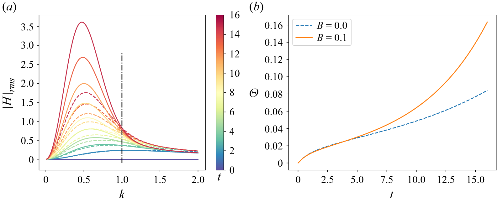
As an illustration, we show a comparison of results for two cases:
 $B=0.0$
and
 $B=0.1$
. The initial spectrum is set to
 $H_i=0$
, and
 $\textit{Oh}=1.0$
,
 $\textit{Th}=0.1$
,
 $L=100$
. The evolution of
 $|H|_{rms}$
in 16 time units is shown in figure 2(a), the corresponding evolution of the surface roughness (
 $\varTheta = \sqrt{({ {1}/{\pi L})\int _0^\infty |H|_{rms}^2 {\rm d}k}}$
) is shown in figure 2(b). It can be seen that the perturbations of small wavenumber (
 $k\lt 1$
) grow faster due to the evaporation–condensation effect. Whereas the perturbations of large wavenumber (
 $k\gt 1$
) grow slower due to the evaporation–condensation effect. The contrasting effect of evaporation–condensation on perturbations of different wavenumber is easy to understand. For a small wavenumber perturbation, the curvature at the trough is larger, hence the evaporation at the trough is enhanced by the Kelvin effect, causing the trough to decrease faster. Whereas for large wavenumber perturbations, the curvature at the crest is larger, hence the evaporation is enhanced at the crest by the Kelvin effect, causing the crest to increase slower. As a result of the dominance of perturbations at
 $k\lt 1$
the evaporation–condensation leads to an enhancement of perturbation growth. Thus in figure 2(b), the surface roughness grows faster at
 $B=0.1$
.
(a) The evolution of
 $|H|_{rms}$
at
 $B=0.0$
(dashed lines) and
 $B=0.1$
(solid lines). The dash-dot line marks the position
 $k=1$
. (b) The evolution of the surface roughness
 $\varTheta$
.

4. Instability in the supersaturated vapour environment
Normally,
 $B$
is very small. For example, for liquid argon at
 $T=84.09\,\mathrm{K}$
, which will be used in MD simulation below, its density is
 $\rho =1398\,\mathrm{kg\,m^{-3}}$
, surface tension
 $\gamma =0.0141\,\mathrm{N\,m^{-1}}$
and the saturation vapour pressure
 $P_0=56\,\mathrm{kPa}$
(Zhao et al. Reference Zhao, Sprittles and Lockerby2019). If the initial radius of the liquid thread is
 $h_0=5\,\mathrm{nm}$
, and
 $\alpha _c$
is assumed to be 1, we can determine the dimensionless parameter
 $B=( {P_0V_0^2}/{\sqrt {{2\pi m (k_BT)}^{3}}})/\sqrt {h_0/\rho \gamma }\approx 3\times 10^{-4}$
. This
 $B$
is so small that the effect of evaporation–condensation is completely negligible. We have also examined
 $B$
for pure water at temperature
 $0^\circ \mathrm{C} \lt T\lt 100^\circ \mathrm{C}$
. We use the International Association for the Properties of Water and Steam interpolation formula (Wagner & Kretzschmar Reference Wagner and Kretzschmar2008) to determine the surface tension, and the Tetens equation (Monteith & Unsworth Reference Monteith and Unsworth2014) to determine the vapour pressure. If the radius of the liquid thread is
 $h_0=5\,\mathrm{nm}$
, the liquid density is fixed at
 $\rho =1000\,\mathrm{kg\,m^{-3}}$
and
 $\alpha _c$
is assumed to be 1, the dimensionless
 $B$
can be determined to be monotonically increasing from
 $6.7\times 10^{-7}$
at
 $0^\circ \mathrm{C}$
to
 $6.2\times 10^{-5}$
at
 $100^\circ \mathrm{C}$
. For liquid propane at
 $185\,\mathrm{K}$
, if we use the density and surface tension data from Kang (Reference Kang2008) (
 $\rho =600\, \mathrm{kg\,m^{-3}}$
,
 $\gamma =0.01\,\mathrm{N\,m^{-1}}$
), and vapour pressure determined from our own additional MD simulation (
 $P_0\approx 23\,\mathrm{kPa}$
), it is found that
 $B\approx 1.3 \times 10^{-4}$
(
 $h_0$
is again set to
 $5\, \mathrm{nm}$
,
 $\alpha _c$
is assumed to be 1). We can see that
 $B$
is usually too small to have a considerable effect on the system. Moreover, the dimensional form of
 $B={\alpha _c P_0V_0^2}/{\sqrt {{2\pi m (k_BT)}^{3}}}$
depends only on the intrinsic properties of the liquid and cannot be easily controlled. Therefore, it is of little practical significance to consider the mass distribution effect caused by the curvature-dependent evaporation in a saturated environment.
On the other hand, the parameter
 $C$
can be controlled by the environmental vapour pressure
 $P_v$
; it can be tuned to be much larger than
 $B$
and may lead to more significant effects on the instability. Thus, in subsequent discussion we focus on the case
 $B \ll C \ll 1$
. The effect of the curvature-dependent evaporation is neglected by setting
 $B=0$
. The basic state (
 $\bar {h},\bar {u}$
) is then determined by setting
 $B$
and all derivative terms with respect to
 $z$
in (2.14), (2.15) to zero and solving the two equations with initial conditions
 $h(z,0)=1,\, u(z,0)=0$
. That is
 $\bar {h} = 1+Ct$
,
 $\bar {u}=0$
(
 $\bar {h}$
is depicted as the red dashed line in figure 1). In contrast to the previous work of Burelbach et al. (Reference Burelbach, Bankoff and Davis1988) on an evaporating/condensing liquid film, it is straightforward to determine the exact basic state for our problem due to the isothermal assumption. Hence, we can let
 $h = 1+Ct+\tilde {h}$
,
 $u=\tilde {u}$
and linearise (2.14), (2.15) to
 \begin{equation} \frac {\partial \tilde {h}}{\partial t} = -\frac {1+Ct}{2}\tilde {u}^{\prime}, \end{equation}
 \begin{equation} \frac {\partial \tilde {u}}{\partial t} = \frac {\tilde {h}^{\prime}}{(1+Ct)^2} + \tilde {h}^{\prime\prime\prime} + 3{\textit{Oh}}\tilde {u}^{\prime\prime} + \sqrt {\frac {6{\textit{Oh}}}{\pi }} {\textit{Th}} \frac {\mathcal{N}^{\prime}}{(1+Ct)}. \end{equation}
Eliminating
 $\tilde {u}$
and applying the finite Fourier transform ((3.4), (3.5)), yields again a second-order ODE
 \begin{equation} \frac {\partial ^2 H}{\partial t^2} + \left (3{\textit{Oh}} k^2-\frac {C}{1+Ct}\right) \frac {\partial H}{\partial t} + \frac {(1+Ct)^2 k^4-k^2}{2(1+Ct)} H = \sqrt {\frac {3{\textit{Oh}}}{2\pi }}{\textit{Th}} k^2 N. \end{equation}
Using the condition
 $C\ll 1$
, we let
 $\varepsilon :=C$
,
 $\tau := \varepsilon t$
and transform the above equation into
 \begin{equation} \varepsilon ^2 \frac {\partial ^2 H}{\partial \tau ^2} + \left (\alpha \varepsilon - \frac {\varepsilon ^2}{1+\tau }\right)\frac {\partial H}{\partial \tau } + \frac {(1+\tau)^2k^4-k^2}{2(1+\tau)} H = \sqrt {\frac {3{\textit{Oh}}}{2\pi }}{\textit{Th}} k^2 N, \end{equation}
where
 $\alpha =3{\textit{Oh}}k^2$
. We first solve the corresponding homogeneous equation
 \begin{equation} \varepsilon ^2 \frac {\partial ^2 H}{\partial \tau ^2} + \left (\alpha \varepsilon - \frac {\varepsilon ^2}{1+\tau }\right)\frac {\partial H}{\partial \tau } + \frac {(1+\tau)^2 k^4-k^2}{2(1+\tau)} H = 0, \end{equation}
with the Wentzel–Kramers–Brillouin (WKB) theory (Bender & Orszag Reference Bender and Orszag1999). In WKB theory, the solution ansatz is
 $H(\tau)\sim \exp [S(\tau)/\delta ]$
,
 $\delta \rightarrow 0$
, where
 $S(\tau)$
is a phase function that could be imaginary (so both dissipative and dispersive behaviours can be characterised). If the solution is dissipative (
 $S(\tau)$
is real),
 $\delta$
is the thickness of the boundary layer; if the solution is dispersive (
 $S(\tau)$
is imaginary),
 $\delta$
is the characteristic scale of the oscillation wavelength. Here,
 $S(\tau)$
depends implicitly on
 $\delta$
, so it is usually expanded as a power series of
 $\delta$
:
 $S(\tau) = \sum _n \delta ^n S_n(\tau)$
. Hence, we assume the form of the approximate solution to be
 \begin{equation} H(\tau)\sim \exp \left [\frac {1}{\delta }\sum _{n=0}^{\infty }\delta ^n S_n(\tau)\right ]\!,\quad \delta \rightarrow 0. \end{equation}
Differentiating
 $H(\tau)$
twice gives
 \begin{equation} \frac {\partial H(\tau)}{\partial \tau }\sim \frac {1}{\delta }\sum _{n=0}^{\infty }\delta ^n S^{\prime}_n(\tau)\exp \left [\frac {1}{\delta }\sum _{n=0}^{\infty }\delta ^n S_n(\tau)\right ]\!,\quad \delta \rightarrow 0, \end{equation}
 \begin{equation} \frac {\partial ^2 H(\tau)}{\partial \tau ^2}\sim \left [\frac {1}{\delta ^2}\left (\sum _{n=0}^{\infty }\delta ^n S^{\prime}_n(\tau)\right)^2 + \frac {1}{\delta }\sum _{n=0}^{\infty }\delta ^nS^{\prime\prime}_n(\tau)\right ]\exp \left [\frac {1}{\delta }\sum _{n=0}^{\infty }\delta ^n S_n(\tau)\right ]\!,\quad \delta \rightarrow 0. \end{equation}
Substituting (4.6), (4.7), (4.8) into (4.5) and dividing off the exponential factors
 \begin{align} \frac {\varepsilon ^2}{\delta ^2}S_0^{\prime 2}+2\frac {\varepsilon ^2}{\delta }S_0^{\prime}S_1^{\prime} + \frac {\varepsilon ^2}{\delta }S_0^{\prime\prime} + \frac {\varepsilon }{\delta }\alpha S_0^{\prime}+\varepsilon \alpha S_1^{\prime} - \frac {\varepsilon ^2}{\delta }\frac {1}{1+\tau }S_0^{\prime} + {\cdots} = -\frac {(1+\tau)^2 k^4-k^2}{2(1+\tau)}. \end{align}
The largest term on the left-hand side of the above equation is either
 $( {\varepsilon ^2}/{\delta ^2})S_0^{\prime 2}$
or
 $( {\varepsilon }/{\delta })\alpha S_0^{\prime}$
, and they must balance the term on the right, so in either case it is required that
 $\delta =\varepsilon$
. Setting
 $\delta =\varepsilon$
, and comparing powers of
 $\varepsilon$
gives a sequence of equations that determines
 $S_0$
,
 $S_1$
,
 ${\cdots}$
. We consider only the first two terms of the sequence:
 $\varepsilon ^0$
 \begin{equation} S_0^{\prime 2} + \alpha S_0^{\prime} + \frac {(1+\tau)k^4}{2}-\frac {k^2}{2(1+\tau)} = 0, \end{equation}
and
 $\varepsilon ^1$
 \begin{align} 2S_0^{\prime}S_1^{\prime}+S_0^{\prime\prime}+\alpha S_1^{\prime} - \frac {1}{1+\tau }S_0^{\prime} = 0. \end{align}
They are solved order by order. However,
 $S_0$
cannot be integrated out, so we seek a local approximation around
 $\tau =0$
and use
 $1/(1+\tau)= 1-\tau + O(\tau ^2)$
to simplify (4.10). This gives
 \begin{align} S_0 =-\frac {1}{2}\alpha \tau \pm \frac {\beta ^3}{6k^4} + O(\tau ^2), \end{align}
where
 $\beta =\sqrt {9{\textit{Oh}}^2k^4 + 2(k^2-k^4)-2(k^2+k^4)\tau }$
. Then
 $S_1$
can be solved from (4.11) to be
 \begin{equation} S_1 = \frac {\pm \alpha \log \frac {\zeta -\beta }{\zeta +\beta }+\zeta \log (1+\tau)-\zeta \log \beta }{2\zeta }, \end{equation}
where
 $\zeta =\sqrt {\alpha ^2+4k^2}$
. Thus, the physical optics approximation of
 $H$
is given by
 \begin{equation} \begin{aligned} H_{LE}(t)&\approx A_1\left (\frac {\zeta -\beta }{\zeta +\beta }\right)^{\frac {\alpha }{2\zeta }}\left (1+\varepsilon t\right)^{\frac {1}{2}} \beta ^{-\frac {1}{2}}\exp \left (-\frac {\alpha t}{2}+\frac {\beta ^3}{6\varepsilon (k^4+k^2)}\right)\\ &\quad+ A_2\left (\frac {\zeta -\beta }{\zeta +\beta }\right)^{-\frac {\alpha }{2\zeta }}\left (1+\varepsilon t\right)^{\frac {1}{2}} \beta ^{-\frac {1}{2}}\exp \left (-\frac {\alpha t}{2}-\frac {\beta ^3}{6\varepsilon (k^4+k^2)}\right)\!, \end{aligned} \end{equation}
where
 $A_1$
and
 $A_2$
are constants that can be determined with initial conditions.
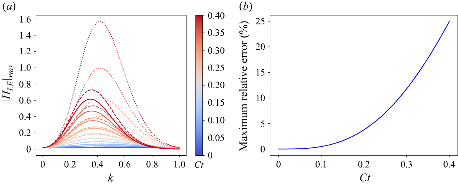
To evaluate the accuracy of the local approximation we conduct a numerical integration on (4.5) using the Scipy integration function odeint, and compare the result with the prediction of (4.14). The initial spectrum
 $H_i$
and Oh have been arbitrarily set to
 $H_i=0.02$
and
 $\textit{Oh}=1.0$
. The integration is computed up to
 $Ct=0.4$
, i.e. the average radius of the liquid thread has increased 40 % due to condensation at the end of the integration. The comparison is presented in figure 3(a). The prediction of (4.14) (solid lines) is in good agreement with the numerical integration result (dashed lines). The deviation becomes large when
 $Ct$
is increased. Figure 3(b) shows that the maximum relative error of (4.14) compared with the numerical integration result is increased up to approximately 25 % at
 $Ct=0.4$
. But when
 $Ct\lt 0.2$
the relative error is less than 5 %. Therefore, we expect that our local approximation is accurate when
 $Ct\lt 0.2$
. The prediction of the classic RP theory is also shown in figure 3 (dotted lines). It can be seen that the inclusion of the condensation effect has significantly impeded the growth of the perturbations. We will discuss this in more detail later.
(a) The evolution of
 $|H_{LE}|_{rms}$
. Solid lines: prediction of (4.14); dashed lines: results determined by numerical integration of (4.5); dotted lines: theoretical prediction of the classic RP theory. (b) The maximum relative prediction error of (4.14) compared with the numerical integration result.

To find the solution of the inhomogeneous (4.3), we solve the Green’s function equation
 \begin{equation} \frac {\partial ^2 G(t,t^{\prime})}{\partial t^2} + \left (\alpha ^2-\frac {\varepsilon }{1+\varepsilon t}\right) \frac {\partial G(t,t^{\prime})}{\partial t} + \frac {(1+\varepsilon t)^2k^4-k^2}{2(1+\varepsilon t)} G(t,t^{\prime}) = \delta (t-t^{\prime}) \end{equation}
with initial conditions:
 \begin{equation} G(t=0,t^{\prime})=0,\quad \partial G/\partial t (t=0,t^{\prime})=0. \end{equation}
In the regions
 $t\lt t^{\prime}$
and
 $t\gt t^{\prime}$
, the solutions have the same form as the solution of the homogeneous equation. In the region
 $t\lt t^{\prime}$
, the initial conditions (4.16) require that the constants
 $A_1$
,
 $A_2$
are both zero. Thus,
 \begin{equation} G(t,t^{\prime}) = 0, \quad t\lt t^{\prime}. \end{equation}
In the region
 $t\gt t^{\prime}$
, we write the solution in the form
 \begin{equation} \begin{aligned} G(t,t^{\prime}) &= A_1(t^{\prime})\left (\frac {\zeta -\beta }{\zeta +\beta }\right)^{\frac {\alpha }{2\zeta }}\left (1+\varepsilon t\right)^{\frac {1}{2}} \beta ^{-\frac {1}{2}} \exp \left (-\frac {\alpha t}{2}+\frac {\beta ^3}{6\varepsilon (k^4+k^2)}\right)\\ &\quad + A_2(t^{\prime}) \left (\frac {\zeta -\beta }{\zeta +\beta }\right)^{-\frac {\alpha }{2\zeta }}\left (1+\varepsilon t\right)^{\frac {1}{2}} \beta ^{-\frac {1}{2}} \exp \left (-\frac {\alpha t}{2}-\frac {\beta ^3}{6\varepsilon (k^4+k^2)}\right)\!,\quad t\gt t^{\prime}. \end{aligned} \end{equation}
The two constants
 $A_1$
,
 $A_2$
are determined by patching. At
 $t=t^{\prime}$
the Green’s function is required to be continuous, and the slope of
 $G(t,t^{\prime})$
is required to have a finite discontinuity
 \begin{equation} G(t^{\prime}_{-},t^{\prime})=G(t^{\prime}_{+},t^{\prime}),\quad \frac {\partial G}{\partial t}(t^{\prime}_{+},t^{\prime}) - \frac {\partial G}{\partial t}(t^{\prime}_{-},t^{\prime}) = 1. \end{equation}
Substituting (4.17), (4.18) into (4.19) the constants
 $A_1(t^{\prime})$
and
 $A_2(t^{\prime})$
can be determined and we find the solution for
 $G(t,t^{\prime})$
to be
 \begin{equation} G(t,t^{\prime}) = \frac {2W(t,t^{\prime})}{D(t^{\prime})\sqrt {\beta }} \exp \left [\frac {-\alpha (t-t^{\prime})}{2}\right ] \sinh \left [\frac {\beta ^3-\beta ^{\prime 3}}{6\varepsilon (k^4+k^2)}-\ln \left (\frac {R(\beta ^{\prime})}{R(\beta)}\right)\right ]\quad t\gt t^{\prime} ,\end{equation}
where
 \begin{equation} W(t,t^{\prime}) = \beta ^{\prime{\frac {3}{2}}}\sqrt {(1+\varepsilon t)(1+\varepsilon t^{\prime})}, \end{equation}
 \begin{equation} D(t^{\prime}) = 2k^4(1+\varepsilon t^{\prime})^2-2k^2\left [1-(\varepsilon t^{\prime})^2\right ] - \alpha ^2(1+\varepsilon t^{\prime}) + \alpha \varepsilon , \end{equation}
 \begin{equation} R(\beta) = \left (\frac {\zeta -\beta }{\zeta +\beta }\right)^{\frac{\alpha }{2\zeta }}, \end{equation}
and
 $\beta =\sqrt {9{\textit{Oh}}^2k^4 + 2(k^2-k^4)-2(k^2+k^4)\varepsilon t^{\prime}}$
. Then the solution of the inhomogeneous equation is
 \begin{equation} H_{fluc} = \sqrt {\frac {3{\textit{Oh}}}{2\pi }}{\textit{Th}} k^2 \int _0^t N(k,t-t^{\prime})G(t,t^{\prime}) {\rm d}t^{\prime}. \end{equation}
The r.m.s. of
 $H_{fluc}$
is given by
 \begin{equation} |H_{fluc}|_{rms} = \sqrt {\langle |H_{fluc}|^2\rangle }= \sqrt {\frac {3{\textit{Oh}}}{2\pi }{\textit{Th}}^2k^4L\int _0^t G^2(t,t^{\prime}){\rm d}t^{\prime}}. \end{equation}
Substituting (4.14), (4.25) into (3.12) we can obtain the evolution of the r.m.s. of the perturbation spectrum.
5. Instability of a short liquid thread
For a long liquid thread the perturbations develop very fast, the thread may break up before the effects of condensation become very significant. To illustrate the effects of condensation more clearly, we consider a short liquid thread whose dimensionless length is close to the critical length in Rayleigh’s theory:
 $2\pi$
, so that the breakup time becomes large and the effects of condensation become significant. For a short liquid thread of fixed length
 $L$
we use a Fourier series to expand the functions
 $\tilde {h}$
and
 $\mathcal{N}$
 \begin{equation} \tilde {h}(z,t) = \sum _{n=-\infty }^{\infty } H^{(n)}(t) \exp \left (nk_0 i z\right), \end{equation}
 \begin{equation} \mathcal{N}(z,t) = \sum _{n=-\infty }^{\infty } N^{(n)}(t)\exp \left (nk_0 i z\right), \end{equation}
where a periodic boundary is assumed and
 $k_0=2\pi /L$
; the expansion coefficients are given by
 \begin{equation} H^{(n)}(t) = \frac {1}{L}\int _0^L \tilde {h}(z,t)\exp (-nk_0iz) {\rm d}z, \end{equation}
 \begin{equation} N^{(n)}(t) = \frac {1}{L}\int _0^L \mathcal{N}(z,t)\exp (-nk_0iz) {\rm d}z. \end{equation}
Following the same procedure described in § 4,
 $H^{(n)}$
is split into two parts:
 $H^{(n)}=H^{(n)}_{LE}(t)+H^{(n)}_{fluc}(t)$
. And the homogeneous solution
 $H^{(n)}_{LE}$
is
 \begin{align} \begin{aligned} H_{LE}^{(n)}(t)&\approx A_1\left (\frac {\zeta -\beta }{\zeta +\beta }\right)^{\frac {\alpha }{2\zeta }}\left (1+\varepsilon t\right)^{\frac {1}{2}} \beta ^{-\frac {1}{2}} \exp \left (-\frac {\alpha t}{2}+\frac {\beta ^3}{6\varepsilon \left [(nk_0)^4+(nk_0)^2\right ]}\right)\\ &\quad + A_2\left (\frac {\zeta -\beta }{\zeta +\beta }\right)^{-\frac {\alpha }{2\zeta }}\left (1+\varepsilon t\right)^{\frac {1}{2}} \beta ^{-\frac {1}{2}} \exp \left (-\frac {\alpha t}{2}-\frac {\beta ^3}{6\varepsilon \left [(nk_0)^4+(nk_0)^2\right ]}\right)\! ,\end{aligned} \end{align}
with
 $\beta = \sqrt {[9{\textit{Oh}}^2-2(1+\varepsilon ^{\prime} t)] (nk_0)^4 + 2(1-\varepsilon ^{\prime} t)(nk_0)^2}$
,
 $\zeta =\sqrt {9{\textit{Oh}}^2(nk_0)^4+4(nk_0)^2}$
. The constants
 $A_1$
and
 $A_2$
can be determined by the initial conditions
 $H_{LE}^{(n)}(t=0) = H_i^{(n)}$
,
 $\partial H_{LE}^{(n)}/\partial t (t=0) = 0$
. The fluctuation-driven part of the Fourier series coefficient is
 \begin{equation} H^{(n)}_{fluc} = \sqrt {\frac {3{\textit{Oh}}}{2\pi }}{\textit{Th}} (nk_0)^2 \int _0^t N^{(n)}(t-t^{\prime})G(t,t^{\prime}) {\rm d}t^{\prime}, \end{equation}
with the Green’s function
 $G(t,t^{\prime})$
the same as (4.20) except that all of the
 $k$
values are replaced by
 $nk_0$
. For a liquid thread whose dimensionless length is around
 $2\pi$
, the wavelength with
 $n=-1$
and
 $1$
are dominant. So we have
 \begin{equation} \tilde {h}(z,t) \approx H^{(-1)}(t)\exp (-k_0iz) + H^{(1)}(t)\exp (k_0iz). \end{equation}
Since
 $H^{(-1)}(t)$
and
 $H^{(1)}(t)$
are conjugate, the perturbation wave on the liquid thread is of sinusoidal form whose amplitude is
 \begin{equation} \tilde {h}_{max}(t) = 2|H^{(1)}_{LE}+H^{(1)}_{fluc}|. \end{equation}
Thus, the r.m.s. of
 $\tilde {h}_{max}(t)$
is
 \begin{equation} \tilde {h}_{max}(t)|_{rms} = 2\sqrt {\left \langle |H^{(1)}_{LE}|^2\right \rangle + \left \langle |H^{(1)}_{fluc}|^2\right \rangle }. \end{equation}
The first term under the square root in (5.9) is easy to calculate, whereas the second term is given by
 \begin{equation} \begin{aligned} \left \langle |H^{(1)}_{fluc}|^2 \right \rangle &= \frac {3{\textit{Oh}}}{2\pi L^2}{\textit{Th}}^2 k_0^4 \int _0^t\int _0^t \int _0^L\int _0^L \begin{aligned}[t]\left \langle \mathcal{N}(z,t-t^{\prime})\mathcal{N}(z^{\prime},t-t^{\prime\prime})\right \rangle \exp [-k_0i(z-z^{\prime})]\\\times G(t,t^{\prime})G(t,t^{\prime\prime}){\rm d}z{\rm d}z^{\prime}{\rm d}t^{\prime}{\rm d}t^{\prime\prime} \end{aligned}\\ &= \frac {3{\textit{Oh}}}{2\pi L}{\textit{Th}}^2 k_0^4 \int _0^t G^2(t,t^{\prime}) {\rm d}t^{\prime}, \end{aligned} \end{equation}
where the correlation relation
 $\langle \mathcal{N}(z,t-t^{\prime}) \mathcal{N}(z^{\prime},t-t^{\prime\prime})\rangle = \delta (z-z^{\prime})\delta (t^{\prime}-t^{\prime\prime})$
has been used for the derivation.
We further try to determine the distribution functions of
 $|H^{(1)}_{fluc}|^2$
and
 $\tilde {h}_{max}(t)$
. The expectation of
 $|H^{(1)}_{fluc}|^2$
is already given by (5.10). To determine the variance of
 $|H^{(1)}_{fluc}|^2$
, we first calculate the expectation of
 $|H^{(1)}_{fluc}|^4$
 \begin{align} \left \langle |H^{(1)}_{fluc}|^4 \right \rangle &=\frac {9{\textit{Oh}}^2}{2\pi ^2L^4}{\textit{Th}}^4 k_0^8 \int _0^t\int _0^t \int _0^t\int _0^t \int _0^L\int _0^L \int _0^L\int _0^L \nonumber\\ &\quad \times \left \langle \mathcal{N}(z,t-t^{\prime})\mathcal{N}(z^{\prime},t-t^{\prime\prime}) \mathcal{N}(z^{\prime\prime},t-t^{\prime\prime\prime})\mathcal{N}(z^{\prime\prime\prime},t-t^{\prime\prime\prime\prime})\right \rangle \nonumber\\ &\quad \times \exp [-k_0i(z-z^{\prime} + z^{\prime\prime}-z^{\prime\prime\prime})] \nonumber\\ &\quad \times G(t,t^{\prime})G(t,t^{\prime\prime})G(t,t^{\prime\prime\prime})G(t,t^{\prime\prime\prime\prime}) \nonumber\\ &\quad \times {\rm d}z{\rm d}z^{\prime}{\rm d}z^{\prime\prime}{\rm d}z^{\prime\prime\prime}{\rm d}t^{\prime}{\rm d}t^{\prime\prime}{\rm d}t^{\prime\prime\prime}{\rm d}t^{\prime\prime\prime\prime} \nonumber\\ &= \frac {9{\textit{Oh}}^2}{2\pi ^2L^2}{\textit{Th}}^4 k_0^8 \left [\int _0^t G^2(t,t^{\prime}) {\rm d}t^{\prime}\right ]^2\! , \end{align}
where the correlation relation (Risken Reference Risken1989)
 \begin{equation} \begin{aligned} &\left \langle \mathcal{N}(z,t-t^{\prime})\mathcal{N}(z^{\prime},t-t^{\prime\prime})\mathcal{N}(z^{\prime\prime},t-t^{\prime\prime\prime})\mathcal{N}(z^{\prime\prime\prime},t-t^{\prime\prime\prime\prime})\right \rangle \\ &\quad = \delta (z-z^{\prime})\delta (t^{\prime}-t^{\prime\prime})\delta (z^{\prime\prime}-z^{\prime\prime\prime})\delta (t^{\prime\prime\prime}-t^{\prime\prime\prime\prime}) \\ &\quad\quad+ \delta (z-z^{\prime\prime})\delta (t^{\prime}-t^{\prime\prime\prime})\delta (z^{\prime}-z^{\prime\prime\prime})\delta (t^{\prime\prime}-t^{\prime\prime\prime\prime})\\ &\quad\quad + \delta (z-z^{\prime\prime\prime})\delta (t^{\prime}-t^{\prime\prime\prime\prime})\delta (z^{\prime}-z^{\prime\prime})\delta (t^{\prime\prime}-t^{\prime\prime\prime}) \end{aligned} \end{equation}
has been used for the derivation.
Thus, the variance of
 $|H^{(1)}_{fluc}|^2$
is
 \begin{equation} \left \langle |H^{(1)}_{fluc}|^4 \right \rangle - \left \langle |H^{(1)}_{fluc}|^2 \right \rangle ^2 = \frac {9{\textit{Oh}}^2}{4\pi ^2L^2}{\textit{Th}}^4 k_0^8 \left [\int _0^t G^2(t,t^{\prime}) {\rm d}t^{\prime}\right ]^2 \!. \end{equation}
It is not a coincidence that the variance of
 $|H^{(1)}_{fluc}|^2$
is the square of its mean. Because the real and imaginary parts of
 $H^{(1)}_{fluc}$
are normal random variables with 0 mean and the same variance (let us denote this variance as
 $\sigma _H^2$
). We can also prove that any linear combination of them is normally distributed, and the cross-correlation coefficient between them is 0. Hence, they are independent random variables. Then,
 $|H^{(1)}_{fluc}|^2$
is actually a random variable of scaled Chi-squared distribution with two degrees of freedom:
 $|H^{(1)}_{fluc}|^2 \sim \sigma _H^2 \chi _2^2$
. Therefore, the mean of
 $|H^{(1)}_{fluc}|^2$
is
 $2\sigma _{H}^2$
and its variance is
 $4\sigma _{H}^4$
. The probability density distribution function of
 $\psi =|H^{(1)}_{fluc}|^2$
is
 \begin{equation} P_\psi (\psi ,t) = \frac {1}{2\sigma ^2_{H}}\exp \left (-\frac {\psi }{2\sigma ^2_H}\right)\! ,\end{equation}
with
 $\sigma ^2_{H}$
determined by comparing
 $\langle |H^{(1)}_{fluc}|^2\rangle = 2\sigma _H^2$
and (5.10)
 \begin{equation} \sigma ^2_{H} = \frac {3{\textit{Oh}}}{4\pi L}{\textit{Th}}^2 k_0^4 \int _0^t G^2(t,t^{\prime}) {\rm d}t^{\prime}. \end{equation}
When the initial perturbations are neglected,
 $\tilde {h}_{max}\approx 2\sqrt {\psi }$
, the probability density function of
 $\tilde {h}_{max}$
is determined from variable transformation to be
 \begin{equation} P_h(\tilde {h}_{max},t) \approx \frac {\tilde {h}_{max}}{4\sigma ^2_H}\exp \left (-\frac {\tilde {h}_{max}^2}{8\sigma ^2_H }\right)\!. \end{equation}
6. Molecular dynamics simulation
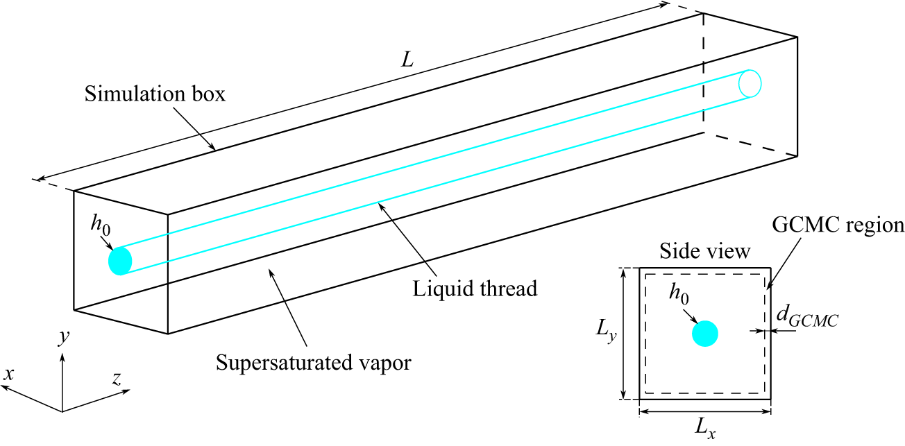
A molecular dynamics simulation of a liquid argon thread (figure 4) with initial radius
 $h_0=5\,\mathrm{nm}$
at
 $T=84.09\, \mathrm{K}$
is conducted to validate our results. The Lennard–Jones 12-6 potential is used to model the interaction among atoms using the energy parameter
 $\varepsilon _{LJ}=0.9938\,\mathrm{kJ\,mol^{-1}}$
and distance parameter
 $\sigma _{LJ}=3.405\,Ã$
. The cutoff radius is set to
 $r_c=15\, Ã$
. The corresponding liquid and saturated vapour density are
 $\rho =1398\,\mathrm{kg\,m^{-3}}$
and
 $\rho _g=3.22\,\mathrm{kg\,m^{-3}}$
(Zhao et al. Reference Zhao, Sprittles and Lockerby2019). The kinematic viscosity of the liquid phase is calculated through the Green–Kubo relation (Frenkel & Smit Reference Frenkel and Smit2023) to be:
 $\nu =1.77\times 10^{-7}\,\mathrm{m^2\,s^{-1}}$
. The surface tension between the liquid and vapour phase is calculated through planar liquid film simulation and the Irving–Kirkwood relation (Kirkwood & Buff Reference Kirkwood and Buff1949; Irving & Kirkwood Reference Irving and Kirkwood1950) to be:
 $\gamma =1.41\times 10^{-2}\,\mathrm{N\,m^{-1}}$
. The initial configurations of the liquid phase and gas phase are extracted from separate bulk liquid and bulk gas simulations under a Nose–Hoover thermostat. We examine several vapour supersaturation conditions:
 $S=2.0,\,3.0,\,4.0$
. The corresponding initial vapour densities are
 $\rho _g = 6.44,\, 9.66,\, 12.88\,\mathrm {kg\,m^{-3}}$
. To sustain the supersaturation condition, a grand canonical Monte Carlo (GCMC) exchange (Frenkel & Smit Reference Frenkel and Smit2023) of atoms with an imaginary ideal gas reservoir with
 $T=84.09\rm \,K$
,
 $P_v=1.11,\, 1.67,\, 2.22\,\mathrm{atm}$
is conducted in the marginal regions (thickness
 $d_{GCMC}=1\,\mathrm{nm}$
) of the simulation box (see figure 4). The whole system is simulated in canonical ensembles (constant particle number N, volume V, and temperature T; NVT), hence the thermal energy released by condensation is removed from the system and the overall temperature of the system is fixed. We have verified that the supersaturation environment only slightly changes the surface tension, thus,
 $\gamma =1.41\times 10^{-2}\,\mathrm{N\,m^{-1}}$
will be used throughout in this article. Periodic boundary condition is applied to all 3 directions of the simulation box. Before the NVT simulation, a very short period (
 $0.03\,\mathrm{ns}$
) of Langevin dynamics simulation is also performed. We change the seed of the random number for the Langevin simulation to repeat the whole simulation many times and get an ensemble average for each simulation condition. We use the open source LAMMPS framework (Thompson et al. Reference Thompson2022) to perform all the MD simulations.
Schematic of the molecular simulation model.

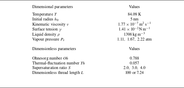
For clarity, we have summarised the physical parameters used in and derived from the MD simulations in table 1. The upper part of the table shows the dimensional parameters (
 $T$
,
 $h_0$
,
 $\nu$
,
 $\gamma$
,
 $\rho$
,
 $P_v$
), the lower part shows the corresponding dimensionless parameters (
 $\textit{Oh}$
,
 $\textit{Th}$
,
 $S$
). The supersaturation ratio
 $S$
is changed due to the variation of the vapour pressure
 $P_v$
. The dimensionless thread length
 $L$
is also changed to examine both very long and short liquid threads.
Physical parameters used in and derived from the MD simulations.

For analysis, the simulation domain is divided into a series of thin slabs along the
 $z$
direction. Particle density
 $\rho _a(z_i,t)$
(including particles in both liquid and vapour phases) in each slab is recorded during the simulation, where
 $z_i$
denotes the
 $z$
coordinate of the centre of the
 $i$
th slab. The vapour density
 $\rho _g(z_i,t)$
is also recorded. Then the radius of the liquid thread at
 $z_i$
is calculated by
 \begin{equation} h(z_i,t)=\sqrt {\frac {L_xL_y(\rho _a-\rho _g)}{\pi (\rho -\rho _g)}}, \end{equation}
where
 $\rho$
is the density of the liquid phase, which we assume to be constant:
 $1398\,\mathrm{kg\,m^{-3}}$
. Discrete Fourier transform is then applied to the sequence of
 $h(z_i,t)$
to get the spectrum
 $H(k,t)$
.
The LAMMPS input scripts and the pre- and post-processing codes used in this study are publicly available on Zenodo (Mo Reference Mo2025).
7. Results and discussion
7.1. Instability of a long liquid thread in supersaturated vapour environment
Molecular dynamics simulation of a long liquid thread in a supersaturated vapour environment. Here,
 $S=3.0$
,
 $C=0.0049$
,
 $L=100$
,
 $\textit{Oh}=0.788$
,
 $\textit{Th}=0.057$
. Dimensional parameters
 $h_0=5\rm\, nm$
,
 $T=84.09\rm \, K$
,
 $P_v=1.67\, \text{atm}$
,
 $L_y=L_z=50\rm \, nm$
. The black lines mark the thread profiles calculated using (6.1). Panels show (a)
 $t=0$
, (b)
 $t=8.98$
, (c)
 $t=17.97$
, (d)
 $t=22.46$
, (e)
 $t=26.95$
, (f)
 $t=31.44$
, (g)
 $t=35.93$
, (h)
 $t=40.42$
.

(a–c) Profile evolutions of a long liquid thread (
 $L=100$
) at different supersaturation ratios. Panels show (a)
 $S=2.0$
, (b)
 $S=3.0$
, (c)
 $S=4.0$
. (d) The evolution of the average thread radius
 $\bar {h}$
at different
 $S$
. The circles are simulation results, the solid lines are linear fits, the dashed lines are theoretical predictions assuming
 $\alpha _c=1$
. The linear fits suggest that
 $\alpha _c=0.545$
,
 $C=0.0015$
at
 $S=2.0$
;
 $\alpha _c=0.901$
,
 $C=0.0049$
at
 $S=3.0$
; and
 $\alpha _c=0.969$
,
 $C=0.0079$
at
 $S=4.0$
. Here,
 $\textit{Oh}=0.788$
,
 $\textit{Th}=0.057$
.

We first consider a long liquid argon thread:
 $L=100$
. We conducted both MD simulation and analytic calculation using (3.12), (4.14), (4.25) to acquire the evolution of the spectrum
 $|H(k,t)|_{rms}$
. Snapshots of an exemplary MD simulation at
 $S=3.0$
are presented in figure 5. We can see from the snapshots that perturbations develop on the surface of the liquid thread as a result of both surface tension and thermal fluctuations and eventually lead to the rupture of the thread. The profile evolutions of the liquid thread at different supersaturation ratios are presented in figure 6(a–c). It can be seen that, the larger the
 $S$
, the faster the increase of the overall radius of the thread. The exact relation between the average thread radius
 $\overline {h}$
and
 $t$
is presented in figure 6(d). The relation is perfectly linear, in accord with the assumption we made in § 4 that the basic state of
 $h$
is a linearly increasing function of
 $t$
. From the linear fits, the exact values of the evaporation/condensation coefficient
 $\alpha _c$
and the dimensionless parameter
 $C$
at different
 $S$
can be determined:
 $\alpha _c=0.545$
,
 $C=0.0015$
at
 $S=2.0$
;
 $\alpha _c=0.901$
,
 $C=0.0049$
at
 $S=3.0$
; and
 $\alpha _c=0.969$
,
 $C=0.0079$
at
 $S=4.0$
. These values change only slightly when the simulations are repeated with different random seeds: the standard deviation for
 $C$
is approximately 0.0001 in all cases. So the correspondence between
 $S$
and
 $\alpha _c$
inferred from figure 6 is used to compute the theoretical predictions for the spectrum evolution.
(a) Analytic
 $|H|_{rms}$
at two instants and different
 $C$
. Here,
 $C$
is varied from 0 to 0.01. (b–d) Comparison between analytic
 $|H|_{rms}$
and MD simulation results. Circles connected by dashed lined: MD results; solid lines: analytic
 $|H|_{rms}$
; dotted lines: theoretical results with the condensation effect not considered (Zhao et al. Reference Zhao, Sprittles and Lockerby2019). Panels show (b)
 $S=2.0$
, (c)
 $S=3.0$
, (d)
 $S=4.0$
. The MD spectrum curves are ensemble averages from 30 simulations. Here,
 $\textit{Oh}=0.788$
,
 $\textit{Th}=0.057$
.

Analytic results of the spectrum at different
 $C$
and comparison of the spectra between MD results and the corresponding analytic results are demonstrated in figure 7. In figure 7(a), the analytic results at two instants (
 $t=12.6$
,
 $t=25.2$
) are presented. The condensation parameter
 $C$
is varied from 0 to 0.01. The initial spectrum
 $H_i$
has been fixed to 0.02 (close to typical values in our MD simulation) to calculate
 $|H_{LE}|_{rms}$
. It can be seen that increasing the condensation parameter
 $C$
causes the perturbations to increase more slowly. The peak of the maximum spectrum shifts to smaller wavenumber. The mechanism of these effects is simple: condensation increases the radius of the liquid thread uniformly, thus making the liquid thread develop as a fatter thread and shifting the spectrum curves to the direction of smaller
 $k$
and a lower spectrum. We compare the MD simulation results with the analytic results in figure 7(b–d). The realistic initial perturbation spectrum
 $|H_i|$
has been extracted from simulations for the calculation of
 $|H_{LE}|_{rms}$
. From (b) to (d) we have increased the supersaturation ratio from
 $S=2$
to
 $S=4$
and the corresponding
 $C$
is increased from
 $C=0.0015$
to
 $C=0.0079$
. We see that the MD results are in very good agreement with the analytic prediction. The larger the
 $S$
the larger the deviation from the classic SLE-RP results of Zhao et al. (Reference Zhao, Sprittles and Lockerby2019). The spectrum is considerably suppressed by the supersaturation environment at high supersaturation ratio. We did not explore higher
 $S$
in MD simulation because increasing the supersaturation ratio further will increase the probability of the occurrence of homogeneous condensation, dramatically complicating the problem. In figure 7, there is a systematic deviation between the analytic and MD results at small wavenumber; it is also present in the work of Zhao et al. (Reference Zhao, Sprittles and Lockerby2019), and is probably a result of the finite-size effect of the MD simulation. There is probably not enough sampling from the finite-length MD system to capture the fluctuations at long wavelength. Another possible origin of the deviation is the fluctuation in the evaporation/condensation flux, which is discussed in detail in Appendix A.
7.2. Instability of a short liquid thread in supersaturated vapour environment
If a liquid thread is short (dimensionless
 $L$
is around
 $2\pi$
), it may take much longer for the perturbations to develop, hence the effect of condensation will become more significant. In this part we consider a liquid thread whose length is
 $L=7.24$
. In this condition, the perturbation with wavenumber
 $k=0.867$
becomes dominant. The MD simulations show that, at different supersaturation ratios
 $S=2.0,\,3.0,\,4.0$
, the evolution of the thread profile could be greatly different (figure 8). In a supersaturated environment the thickness of the thread increases gradually. When
 $S$
is relatively small the thickening does not significantly hinder the growth of perturbations, and the thread could eventually break (figure 8
a). However, larger
 $S$
leads to a faster increase of thickness and could cause the perturbations to be suppressed, as shown in figures 8(b) and 8(c). In figure 8(d) we show that the average thread radius increases linearly, in line with the time-dependent basic state we have used in § 4. From the linear fits, the exact values of the evaporation/condensation coefficient
 $\alpha _c$
and the dimensionless parameter
 $C$
at different
 $S$
are determined:
 $\alpha _c=0.603$
,
 $C=0.0016$
at
 $S=2.0$
;
 $\alpha _c=0.921$
,
 $C=0.0050$
at
 $S=3.0$
; and
 $\alpha _c=0.989$
,
 $C=0.0080$
at
 $S=4.0$
. These values are only slightly different from those we obtained from the long-thread simulations. Using our theory presented in § 5 ((5.9), (5.5), (5.10)), we calculate the evolution of the r.m.s. of the maximum perturbation
 $\tilde {h}_{max}|_{rms}$
and compare it with the MD result. In figure 9(a) the analytic results at different
 $C$
(again we have fixed
 $H_i^{(1)}=0.02$
) are presented. It can be seen that increasing
 $C$
causes the originally exponentially increasing
 $\tilde {h}_{max}|_{rms}$
to transform to a non-monotonic function. At relatively high
 $C$
, the maximum perturbation first increases and then decreases, the liquid thread is completely stabilised by condensation. In figure 9(b–d), we show the comparison between MD results and analytic results. The realistic initial coefficient
 $H_i^{(1)}$
has been extracted from MD simulations and used for the calculation of
 $\langle |H_{LE}^{(1)}|^2\rangle$
. From (b) to (d) the supersaturation ratio is increased from
 $S=2.0$
to
 $S=4.0$
, the corresponding
 $C$
is increased from
 $C=0.0016$
to
 $C=0.0080$
. We can see from the MD data points (coloured circles) and their ensemble averages (dashed lines) that, with the increase of supersaturation ratio, the maximum perturbation is effectively suppressed. At
 $S=2.0$
, the perturbation develops slower than that predicted by the classic SLE-RP theory (Zhao et al. Reference Zhao, Sprittles and Lockerby2019), but it is still relatively fast and there are some cases for which the liquid thread eventually breaks. However, at
 $S=3.0$
and
 $S=4.0$
, the maximum perturbation always first increases and then decreases, suggesting that the liquid thread has been effectively stabilised by the condensation process. This illustrates that, even though the condensation is a slow process, it can significantly alter the instability of short liquid threads. In figure 9(b–d), our analytic predictions (solid lines) based on the MSLE-RP theory agrees well with the ensemble-averaged MD results. Deviations occur mainly at larger
 $t$
and
 $C$
. They arise mainly from the local approximation used in our derivation, which assumes
 $Ct\ll 1$
. The larger the
 $C$
the earlier the assumption
 $Ct\ll 1$
becomes invalid. In figure 9(b–d) there is also a small systematic deviation at small
 $t$
. This deviation originates from the neglect of higher-order Fourier modes. It has been assumed that the first-order Fourier mode is dominant so that
 $\tilde {h}_{max}=2|H^{(1)}|$
, but this is not true at the beginning of the thinning process or if the thread has been stabilised. We have validated that this deviation can be completely eliminated if we extract the r.m.s. of
 $2|H^{(1)}|$
from the MD simulations and compare its evolution with our theoretical prediction (see the inset of figure 9
d). Moreover, the agreement of
 $2|H^{(1)}|$
with the theoretical predictions is also much better than that of
 $\tilde {h}_{max}$
at large
 $t$
, when the thread has already stabilised. This suggests that truncating the Fourier series and neglecting higher-order modes also contributes to the deviations observed at large
 $t$
in figure 9(c–d).
(a–c) Profile evolution of a short liquid thread (
 $L=7.24$
) at different supersaturation ratios. Panels show (a)
 $S=2.0$
, (b)
 $S=3.0$
, (c)
 $S=4.0$
. In (a) the perturbations on the liquid thread develop fast whereas in (b–c) the liquid thread is more stable. (d) The evolution of the average thread radius
 $\bar {h}$
at different
 $S$
. The circles are simulation results, the solid lines are linear fits, dashed lines are theoretical lines assuming
 $\alpha _c=1$
. The linear fits suggest that
 $\alpha _c=0.603$
,
 $C=0.0016$
at
 $S=2.0$
;
 $\alpha _c=0.921$
,
 $C=0.0050$
at
 $S=3.0$
; and
 $\alpha _c=0.989$
,
 $C=0.0080$
at
 $S=4.0$
. Here,
 $\textit{Oh}=0.788$
,
 $\textit{Th}=0.057$
.

(a) The analytic evolution of the r.m.s. of the maximum perturbation magnitude
 $\langle \tilde {h}_{max}\rangle$
of a short liquid thread at different
 $C$
, where
 $C$
is varied from 0 to 0.01. (b–c) Comparison between MD results and analytic results. Coloured circles: data points from MD simulations (120 simulations for (b), 60 simulations for (c) and (d)); dashed lines: ensemble averages (i.e. r.m.s.) from the simulations; solid lines: theoretical results from modified-SLE RP instability (MSLE-RP); dotted lines: theoretical results from SLE RP instability (SLE-RP). The inset of (d) presents the r.m.s. of
 $2|H^{(1)}|$
and its comparison with the corresponding theoretical prediction. Panels show (b)
 $S=2.0$
, (c)
 $S=3.0$
, (d)
 $S=4.0$
. Here,
 $\textit{Oh}=0.788$
,
 $\textit{Th}=0.057$
.

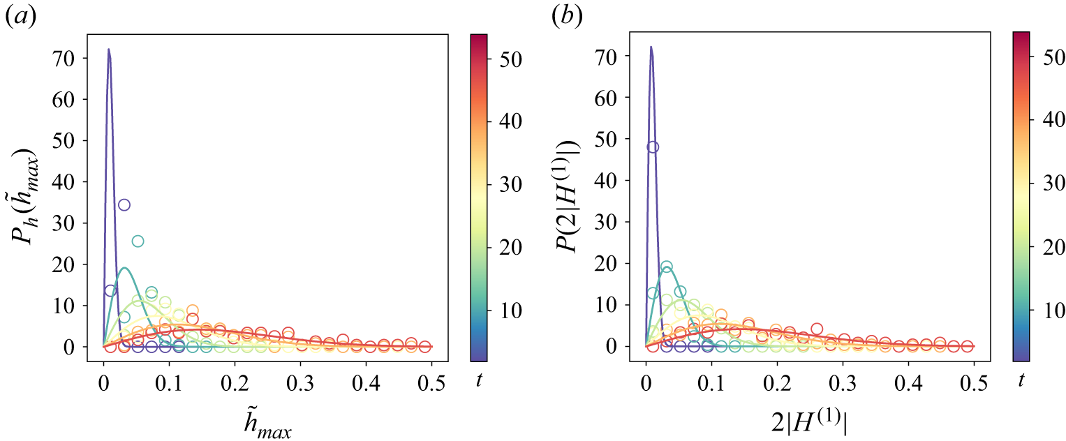
(a) Probability density function of the maximum perturbation magnitude
 $\tilde {h}_{max}$
. (b) Probability density function of the first-order perturbation magnitude
 $2|H^{(1)}|$
. Solid lines: analytic results. Circles: statistics from 120 MD simulations.
 $S=2.0$
,
 $C=0.0016$
.

We calculate the probability density function of the perturbation magnitude
 $\tilde {h}_{max}$
from 120 MD simulations at
 $S=2.0$
and present the results in figure 10(a). The theoretical prediction of (5.16) is also shown. It can be seen that the peaks of the probability density functions decrease with the increase of time and shift to larger
 $\tilde {h}_{max}$
. This is in accord with the monotonically increasing behaviour of
 $\tilde {h}_{max}|_{rms}$
presented in figure 9(b). The MD simulation results and the analytic results are in qualitative agreement. The large deviations at small time are mainly due to the neglect of higher-order Fourier modes. This is manifested in figure 10(b), where the first-order perturbation magnitude
 $2|H^{(1)}|$
has been extracted from the MD results and compared with (5.16). It can be seen that much better agreement is obtained. Therefore, the MD results validate our theoretical prediction that when the first-order Fourier mode is dominant the square of the maximum perturbation magnitude follows the scaled Chi-squared distribution.
8. Conclusions
We have proposed a modified SLE to consider the effects of evaporation and condensation on the instability of nano liquid threads. Through stability analysis incorporating both thermal fluctuations and evaporation–condensation, we show that the effect of the curvature-dependent evaporation is to enhance the growth of perturbations with small wavenumbers (
 $k\lt 1$
) but impede those with large wavenumber (
 $k\gt 1$
). However, in reality, the total effect of the curvature-dependent evaporation is usually very small and makes very little contribution to the instability. In a supersaturated vapour environment, condensation is dominant. Stability analysis and MD simulations both show that the growth of perturbations is considerably impeded by the condensation. The spectrum curves of the perturbations shift to smaller
 $k$
and lower magnitude. The effect of condensation is most clearly manifested on short nano liquid threads whose dimensionless lengths are around
 $2 \pi$
and the perturbation at
 $k\approx 1$
is dominant. Even though condensation is a slow process it can completely alter the stability of the short liquid thread, rendering an originally unstable thread stable. With the increase of the supersaturation ratio, the expectation of the maximum perturbation transforms from an exponentially increasing function of time to be a non-monotonic function of time. When the first-order Fourier mode is dominant, the square of the maximum perturbation follows the scaled Chi-squared distribution with two degrees of freedom.
It has been argued by previous researchers (Kang & Landman Reference Kang and Landman2007; Gopan & Sathian Reference Gopan and Sathian2014) that near the breakup point evaporation–condensation will transform the pinch-off profile from a symmetric double-cone shape to an asymmetric long-thread shape. It is necessary to re-evaluate the pinch-off profile problem in a non-saturated environment under the MSLE framework we propose here, which we believe is more physically reasonable than that of Kang & Landman (Reference Kang and Landman2007). This can be an interesting future research direction. Besides this, there are several other potential research directions: (i) to predict the breakup time of nano liquid threads in a supersaturated environment. As we have seen in this article, the condensation tends to stabilise the liquid thread. At some critical condensation rates, the liquid thread will either break quickly or will never break. The corresponding breakup time will be either finite or infinity. It is interesting to investigate the probability density function of the breakup time. It is actually a classic problem of finding the first passage time or exit time. The conventional technique of setting an absorbing boundary condition and solving the Fokker–Planck equation (Risken Reference Risken1989; Jacobs Reference Jacobs2010) for the system may be tried. Finding the Fokker–Planck equation of the SLE is challenging but will greatly help us elucidate the stochastic breakup behaviour of nano liquid threads. (ii) To consider the effects of heat transfer and phase change. These factors may impact the stability through the dependence of thermal fluctuations on the temperature. To account for the effects of heat transfer and phase change the SLE needs to be re-derived. The governing system of this problem is similar to the one for evaporating/condensing liquid film studied by Burelbach et al. (Reference Burelbach, Bankoff and Davis1988). It constitutes the Landau–Lifshitz–Navier–Stokes equation, mass and energy equations in the fluid, the jump mass and energy balance equations at the interface, the normal- and shear-stress boundary conditions and the constitutive relation from the one-sided model. This governing system could be tackled with the lubrication approximation to acquire a new SLE. (iii) To incorporate the evaporation–condensation in thin film SLEs (Grün et al. Reference Grün, Mecke and Rauscher2006; Zhang et al. Reference Zhang, Sprittles and Lockerby2020) and investigate its effects on the instability of nano liquid films. Because the growth of instability on liquid films is usually slower than that on liquid threads, we believe that the effect of evaporation–condensation could be more significant for the instability of nano liquid films. The curvature-dependent evaporation may have more interesting influences on nano liquid films. (iv) Further discussion on the evaporation–condensation model. Even though the Hertz–Knudsen model successfully describes the evaporation–condensation process for the specific case we study, a liquid thread in its own vapour, the application of the diffusion-limited model can be further discussed. The diffusion-limited model is widely used and well tested at the nanoscale (Chatwell, Heinen & Vrabec Reference Chatwell, Heinen and Vrabec2019), and is probably more appropriate if there is inert gas surrounding the liquid thread. It is interesting to further investigate the instability and breakup of liquid threads if the evaporation–condensation is diffusion limited.
Funding
This work is supported by the National Natural Science Foundation of China (Grant Nos. 12302323, 12272026 and 52425606), the Zhejiang Provincial Natural Science Foundation of China (Grant No. ZCLMS26A0203), the Science Foundation of Aeronautics (Grant No. 2024M039051004) and the National Key Lab of Aerospace Power System and Plasma Technology (Grant No. 110329JC36025060002).
Declaration of interests
We declare we have no competing interests.
Data availability statement
The LAMMPS input scripts and the pre- and post-processing codes are publicly available on Zenodo: https://doi.org/10.5281/zenodo.17946388. The raw simulation data are not publicly available due to their large size but can be generated using the provided scripts.
Appendix A. Effect of the fluctuations in the evaporation–condensation flux
For an ideal gas, the motions of different molecules are spatially and temporally uncorrelated, hence molecules condensing onto the interface are all independent. It is therefore a Poisson process. For a small area
 $\Delta A$
on the interface, during a time interval
 $\Delta t$
, the total number
 $N_c$
of molecules condensed to the liquid follows the Poisson distribution
 $N_c\sim \text{Pois}(\lambda _c)$
with mean value given by
 $\lambda _c = \text{E}(N_c)= {\alpha _c P_v \Delta A\Delta t}/{\sqrt {2\pi m k_B T}}$
. For a Poisson distribution, the variance is the same as the mean value. Hence,
 $\text{Var}(N_c)=\lambda _c$
. For the evaporation flux, we can follow the same analysis process and find that the total number
 $N_e$
of molecules evaporated from the area
 $\Delta A$
in the time interval
 $\Delta t$
follows the Poisson distribution
 $N_e\sim \text{Pois}(\lambda _e)$
, with
 $\lambda _e = \text{E}(N_e)= {\alpha _c P_s \Delta A\Delta t}/{\sqrt {2\pi m k_B T}}$
,
 $\text{Var}(N_e)=\lambda _e$
. Then, the net evaporation–condensation molecule number
 $N_{ec}$
, which is the difference between the two random numbers
 $N_e$
and
 $N_c$
, follows the Skellam distribution. Its mean value is
 \begin{equation} \text{E}(N_{ec})=\lambda _e-\lambda _c = \frac {\alpha _c(P_s-P_v) \Delta A\Delta t}{\sqrt {2\pi m k_B T}}, \end{equation}
its variance is
 \begin{equation} \text{Var}(N_{ec})=\lambda _e+\lambda _c = \frac {\alpha _c(P_s+P_v) \Delta A\Delta t}{\sqrt {2\pi m k_B T}}. \end{equation}
Since the net evaporation–condensation number flux is
 $J = N_{ec}/\Delta A\Delta t$
, the mean value and the variance of
 $J$
are
 \begin{equation} \bar {J}=\text{E}(J)=\frac {\alpha _c(P_s-P_v)}{\sqrt {2\pi m k_B T}}, \end{equation}
 \begin{equation} \text{Var}(J) = \frac {\alpha _c(P_s+P_v)}{\Delta A\Delta t\sqrt {2\pi m k_B T}}. \end{equation}
For our axisymmetric liquid thread problem
 $\Delta A=2\pi h \Delta z$
.
Due to the spatial and temporal independence of the events for molecules condensing onto and evaporating from the interface, we can model the net evaporation–condensation number flux with a white noise
 \begin{equation} J(z,t) = \bar {J}(z,t)+j(z,t), \end{equation}
where
 $\langle j(z,t)j(z^{\prime},t^{\prime})\rangle = 2D(z) \delta (t-t^{\prime})\delta (z-z^{\prime})$
and
 $D$
is the noise strength. We can use the fluctuation term
 $j$
to calculate the variance of the net evaporation–condensation molecule number in a small area
 $\Delta A = 2\pi h\Delta z$
and time interval
 $\Delta t$
 \begin{equation} \begin{aligned} \text{Var}(N_{ec}) &= \int _{z}^{z+\Delta z}\int _t^{t+\Delta t} \int _{z}^{z+\Delta z}\int _t^{t+\Delta t} (2\pi h)^2 \left \langle j(z,t) j(z^{\prime},t^{\prime}) \right \rangle {\rm d}t {\rm d}z{\rm d}t^{\prime} {\rm d}z^{\prime}\\ &= \int _{z}^{z+\Delta z}\int _t^{t+\Delta t} \int _{z}^{z+\Delta z}\int _t^{t+\Delta t} 8(\pi h)^2 D\delta (t-t^{\prime})\delta (z-z^{\prime}) {\rm d}t {\rm d}z{\rm d}t^{\prime} {\rm d}z^{\prime}\\ &= 8(\pi h)^2D\Delta z \Delta t, \end{aligned} \end{equation}
where we have chosen
 $\Delta z$
to be small enough so that
 $h(z)$
and
 $D(z)$
are almost unchanged. Then the variance of the flux
 $J$
is
 \begin{equation} \text{Var} (J) = \frac {2D}{\Delta z\Delta t}. \end{equation}
Comparing (A4) and (A7) the noise strength is determined
 \begin{equation} D = \frac {\alpha _c(P_s+P_v)}{4\pi h \sqrt {2\pi m k_B T}}. \end{equation}
The volume flux
 $J_v = JV_0$
, where
 $V_0$
is the molecule volume. Substituting
 $J_v=JV_0=(\bar {J}+j)V_0$
,
 $j=\sqrt {2D} \mathcal{N}$
, (A3), (A8) and the Kelvin relation (2.3) into (2.10) we obtain the mass equation with the fluctuations in the evaporation–condensation flux considered
 \begin{equation} \frac {\partial h}{\partial t} = - uh^{\prime} - \frac {u^{\prime}h}{2}-\frac {\alpha _c P_0V_0 \left (1+\dfrac {\kappa \gamma V_0}{k_B T}-S\right)}{\sqrt {2\pi mk_B T}} + V_0\left [\frac {\alpha _c P_0 \left (1+\dfrac {\kappa \gamma V_0}{k_B T}+S\right)}{2\pi h \sqrt {2\pi mk_B T}}\right ]^{\frac {1}{2}}\mathcal{N}, \end{equation}
where
 $\mathcal{N}$
is white noise with correlation function
 $\langle \mathcal{N}(z,t) \mathcal{N}(z^{\prime},t^{\prime})\rangle = \delta (z-z^{\prime})\delta (t-t^{\prime})$
. Defining
 $B:= {\alpha _c P_0V_0^2}/{\sqrt {{2\pi m (k_BT)}^{3}}}$
,
 $C:= {\alpha _c P_0V_0(S-1)}/{\sqrt {2\pi mk_B T}}$
,
 $F:= {\alpha _c P_0V_0^3}/{\sqrt {{2\pi m (k_BT)}^{3}}}$
,
 $G:= {\alpha _c P_0V_0^2(S+1)}/{\sqrt {2\pi mk_B T}}$
, (A9) becomes
 \begin{equation} \frac {\partial h}{\partial t} = - uh^{\prime} - \frac {u^{\prime}h}{2}-B\gamma \kappa + C + \left (\frac {F\gamma \kappa +G} {2\pi h}\right)^{\frac {1}{2}}\mathcal{N}. \end{equation}
Using the non-dimensionalisation relations presented in (2.13) along with two additional non-dimensionalisation relations
 $F = {F^*}/{\sqrt {h_0^{7}/\rho \gamma }}$
,
 $G = {G^*}/{\sqrt {\gamma h_0^5/\rho }}$
, (A10) is non-dimensionalised to be
 \begin{equation} \frac {\partial h}{\partial t} = - uh^{\prime} - \frac {u^{\prime}h}{2}-B\kappa + C + \left (\frac {F\kappa +G} {2\pi h}\right)^{\frac {1}{2}}\mathcal{N}. \end{equation}
We discuss the cases
 $B=C$
and
 $C\gg B$
separately.
A.1. In a saturated environment
 $(B=C)$

We first linearise (A11) to be
 \begin{equation} \frac {\partial \tilde {h}}{\partial t} = -\frac {\tilde {u}^{\prime}}{2} + B(\tilde {h}+\tilde {h}^{\prime\prime}) + \sqrt {\frac {F+G}{2\pi }}\mathcal{N}_1, \end{equation}
where the empirical condition
 $F\ll 1$
has been used to simplify the equation. Combining (A12) with the linearised momentum equation
 \begin{equation} \frac {\partial \tilde {u}}{\partial t} = \tilde {h}^{\prime} + \tilde {h}^{\prime\prime\prime} + 3{\textit{Oh}}\tilde {u}^{\prime\prime} + \sqrt {\frac {6{\textit{Oh}}}{\pi }} {\textit{Th}} \mathcal{N}_2^{\prime}, \end{equation}
we can eliminate
 $\tilde {u}$
and obtain an equation with respect to
 $\tilde {h}$
 \begin{align} \nonumber\frac {\partial ^2 \tilde {h}}{\partial t^2} &= B\frac {\partial \tilde {h}}{\partial t} + (B+3{\textit{Oh}})\frac {\partial \tilde {h}^{\prime\prime}}{\partial t} - \left (\frac {1}{2}+3{\textit{Oh}} B\right)\left (\tilde {h}^{\prime\prime}+\tilde {h}^{\prime\prime\prime\prime}\right)\\ &\quad +K\frac {\partial \mathcal{N}_1}{\partial t} - 3{\textit{Oh}}K\mathcal{N}_1^{\prime\prime}- \sqrt {\frac {3{\textit{Oh}}}{2\pi }}{\textit{Th}} \mathcal{N}_2^{\prime\prime}, \end{align}
where
 $K=\sqrt {(F+G)/2\pi }$
and we have use
 $\mathcal{N}_1$
and
 $\mathcal{N}_2$
to distinguish the two independent white noises in the mass and momentum equations. Since
 $K \ll 1$
, the second last term of (A14) is much smaller than the last term, we can neglect it and obtain
 \begin{equation} \frac {\partial ^2 \tilde {h}}{\partial t^2} = B\frac {\partial \tilde {h}}{\partial t} + (B+3{\textit{Oh}})\frac {\partial \tilde {h}^{\prime\prime}}{\partial t} - \left (\frac {1}{2}+3{\textit{Oh}}B\right)\left (\tilde {h}^{\prime\prime}+\tilde {h}^{\prime\prime\prime\prime}\right) +K\frac {\partial \mathcal{N}_1}{\partial t} - \sqrt {\frac {3{\textit{Oh}}}{2\pi }}{\textit{Th}} \mathcal{N}_2^{\prime\prime}. \end{equation}
Applying the finite Fourier transform ((3.4), (3.5)) to the above equation gives
 \begin{equation} \begin{aligned}&\frac {d^2 H}{{\rm d} t^2} + \left (k^2(B+3{\textit{Oh}})-B\right)\frac {{\rm d}H}{{\rm d}t} + \left (\frac {1}{2}+3{\textit{Oh}}B\right)(k^4-k^2)H\\ &\qquad =K\frac {\partial N_1}{\partial t}+\sqrt {\frac {3{\textit{Oh}}}{2\pi }}{\textit{Th}} k^2 N_2. \end{aligned}\end{equation}
We analyse (A16) in the frequency domain. After a Fourier transform in the time domain, the two terms on the right-hand side of (A16) become
 $i\omega K\hat {N}_1$
and
 $(\sqrt {{3{\textit{Oh}}}/{2\pi }}){\textit{Th}} k^2 \hat {N}_2$
, where
 $\omega$
is the angular frequency and
 $\hat {N}_1$
and
 $\hat {N}_2$
are the spectra of the white noises. Normally we have
 $K\ll \sqrt {3 {\textit{Oh}}/\pi }{\textit{Th}}$
. So the first term is comparable to the second term only at high frequency or at small wavenumber. But the second-order ODE represented by (A16) is an over-damped system with no oscillation, all high frequency modes are suppressed. The frequency of the dominant mode is close to 0. Hence, the relation
 $\omega K\ll \sqrt {3 {\textit{Oh}}/\pi }{\textit{Th}}k^2$
is always valid except at very small wavenumber. As long as
 $\omega K\ll \sqrt {3 {\textit{Oh}}/\pi }{\textit{Th}}k^2$
, the effect of the fluctuations in the evaporation–condensation flux is negligible. For argon at
 $T=84.09\ \mathrm{K}$
,
 $S=1.0$
,
 $h_0=5\ \mathrm{nm}$
, we have
 $K\approx 0.0001$
,
 $\textit{Oh}=0.788$
,
 $\textit{Th}=0.057$
. Therefore,
 $\omega K\ll \sqrt {3 {\textit{Oh}}/\pi }{\textit{Th}}k^2$
is well satisfied except at
 $k\approx 0$
. But at
 $k\approx 0$
, the whole right-hand side of (A16) is very small and negligible. Therefore, we can safely neglect the effect of the fluctuations in the evaporation–condensation flux.
A.2. In a supersaturated environment
$(B\ll C)$

Using the empirical condition
 $G\ll 1$
and assuming
 $h=1+Ct+\tilde {h}$
and
 $Ct\ll 1$
(focusing only on the initial stage), (A11) can be linearised to be
 \begin{equation} \frac {\partial \tilde {h}}{\partial t} = -\frac {1+Ct}{2}\tilde {u}^{\prime} + \sqrt {\frac {G}{2\pi }}\mathcal{N}_1. \end{equation}
Combining this equation with the linearised momentum equation
 \begin{equation} \frac {\partial \tilde {u}}{\partial t} = \frac {\tilde {h}^{\prime}}{(1+Ct)^2} + \tilde {h}^{\prime\prime\prime} + 3{\textit{Oh}}\tilde {u}^{\prime\prime} + \sqrt {\frac {6{\textit{Oh}}}{\pi }} {\textit{Th}} \frac {\mathcal{N}_2^{\prime}}{(1+Ct)}, \end{equation}
we can eliminate
 $\tilde {u}$
and obtain
 \begin{equation} \begin{aligned} & \frac {\partial ^2\tilde {h}}{\partial t^2} - \frac {C}{1+Ct}\frac {\partial {\tilde {h}}}{\partial t} + \frac {\tilde {h}^{\prime\prime}}{2(1+Ct)} + \frac {1+Ct}{2}\tilde {h}^{\prime\prime\prime\prime} - 3{\textit{Oh}}\frac {\partial \tilde {h}^{\prime\prime}}{\partial t} \\ &\quad+ \sqrt {\frac {3{\textit{Oh}}}{2\pi }} {\textit{Th}} \mathcal{N}_2^{\prime\prime} + \frac {C}{1+Ct}\sqrt {\frac {G}{2\pi }} \mathcal{N}_1 - \sqrt {\frac {G}{2\pi }} \frac {\partial \mathcal{N}_1}{\partial t} + 3{\textit{Oh}}\sqrt {\frac {G}{2\pi }}\mathcal{N}_1^{\prime\prime} = 0. \end{aligned} \end{equation}
Applying the finite Fourier transform to the above equation, we have
 \begin{equation} \begin{aligned} & \frac {\partial ^2 H}{\partial t^2} + \left (3{\textit{Oh}} k^2-\frac {C}{1+Ct}\right) \frac {\partial H}{\partial t} + \frac {(1+Ct)^2 k^4-k^2}{2(1+Ct)} H \\ &\quad = \sqrt {\frac {3{\textit{Oh}}}{2\pi }}{\textit{Th}} k^2 N_2 + \left (3{\textit{Oh}}k^2 - \frac {C}{1+Ct}\right)\sqrt {\frac {G}{2\pi }} N_1 + \sqrt {\frac {G}{2\pi }}\frac {\partial N_1}{\partial t}. \end{aligned} \end{equation}
We again analyse the above system in the frequency domain. It is evident that if
 $3\textit{Oh}(\sqrt {{G}/{2\pi }}) \ll (\sqrt { {3{\textit{Oh}}}/{2\pi }}){\textit{Th}}$
, and
 $(\sqrt { {G}/{2\pi }})\omega \ll (\sqrt { {3{\textit{Oh}}}/{2\pi }}) {\textit{Th}} k^2$
, the terms with
 $N_1$
can be neglected. The former relation is satisfied since
 $G$
is very small compared with
 $\textit{Oh}$
and
 $\textit{Th}$
. But for the later relation, it will be valid only if the frequency
 $\omega$
is not large and
 $k$
is not close to 0. Since the second-order ODE represented by (A20) is an over-damped system with no oscillation, the dominant frequency is close to 0. Hence,
 $(\sqrt { {G}/{2\pi }})\omega \ll (\sqrt { {3{\textit{Oh}}}/{2\pi }}) {\textit{Th}} k^2$
is satisfied except at
 $k\approx 0$
. In reality, for a liquid argon thread at
 $T=84.09\ \mathrm{K}$
,
 $h_0=5\ \mathrm{nm}$
and
 $S=2.0$
, we have
 $G \approx 10^{-6}$
,
 $\textit{Oh}=0.788$
,
 $\textit{Th}=0.057$
. The relation
 $(\sqrt { {G}/{2\pi }})\omega \ll (\sqrt { {3{\textit{Oh}}}/{2\pi }}) {\textit{Th}} k^2$
is well satisfied except at
 $k\approx 0$
. But if
 $k\approx 0$
the whole right-hand side of (A20) is very small and negligible. Thus, the effect of the fluctuations in the evaporation–condensation flux can be neglected.
Therefore, we can see that, in both the saturated and supersaturated cases, the contribution of the fluctuations to the evaporation–condensation flux is normally very small compared with the contribution of the stress fluctuations. The exception occurs at
 $k\approx 0$
, where the contribution of the stress fluctuations also becomes very small. We have observed small systematic deviations of the spectrum at very low wavenumber in figure 7. Besides of the finite-size effect, the neglect of the fluctuations in the evaporation–condensation flux may have also contributed to the deviations.