1 Introduction
Yield-stress fluids are shear-thinning non-Newtonian fluids. They effectively flow only for a sufficiently large applied stress (Bird, Armstrong & Hassager Reference Bird, Armstrong and Hassager1987; Nguyen & Boger Reference Nguyen and Boger1992; Balmforth, Frigaard & Ovarlez Reference Balmforth, Frigaard and Ovarlez2014; Coussot Reference Coussot2014; Bonn et al. Reference Bonn, Denn, Berthier, Divoux and Manneville2017). At lower stresses, they are predominantly solid. Their applications include fire suppression, jet and spray printing, painting, coatings, food processing and direct-write 3D printing (Luu & Forterre Reference Luu and Forterre2009; Sun & Gunasekaran Reference Sun and Gunasekaran2009; Blackwell Reference Blackwell2017; Nelson & Ewoldt Reference Nelson and Ewoldt2017; Nelson et al. Reference Nelson, Schweizer, Rauzan, Nuzzo, Vermant and Ewoldt2019). Drop, jet and spray impacts of these complex fluids differ qualitatively and quantitatively from impact tests with Newtonian fluids. Extensive literature exists for wide-ranging scenarios of fluid impacts with Newtonian fluids (Rein Reference Rein1996; Cossali, Coghe & Marengo Reference Cossali, Coghe and Marengo1997; Wang & Chen Reference Wang and Chen2000; Sivakumar & Tropea Reference Sivakumar and Tropea2002; Josserand & Zaleski Reference Josserand and Zaleski2003; Vander Wal, Berger & Mozes Reference Vander Wal, Berger and Mozes2005a,Reference Vander Wal, Berger and Mozesb), but studies for non-Newtonian fluids, especially yield-stress fluids, are more limited (Nigen Reference Nigen2005; Luu & Forterre Reference Luu and Forterre2009; Guémas, Marín & Lohse Reference Guémas, Marín and Lohse2012; Blackwell et al. Reference Blackwell, Deetjen, Gaudio and Ewoldt2015; Blackwell, Nadhan & Ewoldt Reference Blackwell, Nadhan and Ewoldt2016; Blackwell et al. Reference Blackwell, Deetjen, Gaudio and Ewoldt2017; Oishi, Thompson & Martins Reference Oishi, Thompson and Martins2019). Researchers have previously studied the impact of various shear-thinning and yield-stress fluid droplets on dry surfaces (German & Bertola Reference German and Bertola2009; Luu & Forterre Reference Luu and Forterre2009) and proposed scaling laws predicting different outcomes of the impacts. Fluids tested were mainly clays such as Kaolin and Bentonite and soft glasses such as Carbopol, as the yield-stress fluids. More weakly shear-thinning fluids (those without an apparent yield stress) tested were formulations of xanthan gum in water (German & Bertola Reference German and Bertola2009). Some of these scaling laws have also been verified experimentally for Carbopol (Guémas et al. Reference Guémas, Marín and Lohse2012), including water-entry problems (Jalaal, Kemper & Lohse Reference Jalaal, Kemper and Lohse2019).
Experiments studying yield-stress fluid drop impacts on films, relevant to spray coating and sequential drop impact, have been lacking. Only recently has this been addressed by Blackwell et al. in a series of works (Blackwell et al. Reference Blackwell, Deetjen, Gaudio and Ewoldt2015, Reference Blackwell, Nadhan and Ewoldt2016, Reference Blackwell, Deetjen, Gaudio and Ewoldt2017). They tested drops of aqueous suspensions of polymeric microgel particles (Carbopol 940, or simply ‘Carbopol’) impacting horizontal substrates coated with the same material and proposed an empirical non-dimensional scaling law for predicting stick–splash behaviour taking into account the most dominant forces (inertial and dissipative flow effects). Such flow conditions and impact configurations are common in industrial processes, and it is surprising that no comprehensive literature exists that seeks to model, or at least heuristically predict, the outcomes of drop impact events on coatings. Extensive studies that explore the general behaviour of a broad class of complex fluids in scientifically relevant configurations are few and far between. Although the dimensionless group proposed is general for yield-stress fluids (agnostic to chemistry and material microstructure), it has only been tested with Carbopol, which is a soft, jammed glassy system. Two key types of microstructure create a yield-stress fluid (Nelson & Ewoldt Reference Nelson and Ewoldt2017), and we seek to test this group for the other important category of yield-stress fluid, gels/attractive particulate networks, for which we use aqueous clay particle suspensions of Laponite RD (or ‘Laponite’ for short). We look to develop scaling laws or dimensionless parameters that can help predict the behaviour of these complex fluids in such fluid flow scenarios. The complexity of impacts on coated surfaces coupled with additional stresses and forces that come into play when dealing with yield-stress fluids pose a challenge for an accurate, rigorous and reproducible study.
Here, we study and test a proposed scaling argument (Blackwell et al. Reference Blackwell, Deetjen, Gaudio and Ewoldt2015) with a different yield-stress fluid (Laponite clay, figure 1a,b) with a significantly different microstructure than a previously studied fluid (Carbopol). We test if it can predict stick–splash behaviour when drops impact substrates coated with the same materials. We look to map impact behaviour to the process parameters using a dimensionless group similar to the one used earlier for Carbopol (Blackwell et al. Reference Blackwell, Deetjen, Gaudio and Ewoldt2015), and to see if similar results are obtained. This group is a comparison between inertial forces and total dissipative flow forces, and is expressed in its most general form as
 $$\begin{eqnarray}\text{IF}\left(\frac{D}{t}\right)\equiv \frac{\unicode[STIX]{x1D70C}V^{2}}{\unicode[STIX]{x1D70E}(\dot{\unicode[STIX]{x1D6FE}}_{char})}\left(\frac{D}{t}\right),\end{eqnarray}$$
where  $\unicode[STIX]{x1D70E}$ is the dissipative flow stress, which is a function of
 $\dot{\unicode[STIX]{x1D6FE}}_{char}$, a characteristic shear rate during drop impact. The specific functional form of
 $\unicode[STIX]{x1D70E}$ depends on the choice of a suitable rheological constitutive equation relevant to the material studied. We shall be testing three constitutive equations for yield-stress fluids, which give us the dimensionless groups of the forms
 $$\begin{eqnarray}\displaystyle & \displaystyle \text{IF}\left(\frac{D}{t}\right)\equiv \frac{\unicode[STIX]{x1D70C}V^{2}}{\unicode[STIX]{x1D70E}_{y}+\unicode[STIX]{x1D702}_{\infty }V/t}\left(\frac{D}{t}\right), & \displaystyle\end{eqnarray}$$
 $$\begin{eqnarray}\displaystyle & \displaystyle \text{IF}\left(\frac{D}{t}\right)\equiv \frac{\unicode[STIX]{x1D70C}V^{2}}{\unicode[STIX]{x1D70E}_{y}+K(V/t)^{n}+\unicode[STIX]{x1D702}_{\infty }V/t}\left(\frac{D}{t}\right), & \displaystyle\end{eqnarray}$$
 $$\begin{eqnarray}\displaystyle & \displaystyle \text{IF}\left(\frac{D}{t}\right)\equiv \frac{\unicode[STIX]{x1D70C}V^{2}}{\unicode[STIX]{x1D70E}_{y}+K(V/t)^{0.5}+\unicode[STIX]{x1D702}_{\infty }V/t}\left(\frac{D}{t}\right), & \displaystyle\end{eqnarray}$$
 $n=0.5$) models respectively (Souza Mendes & Dutra Reference Souza Mendes and Dutra2004). The group IF is a ratio of stresses, while
 $\text{IF}(D/t)$ is a ratio of forces, based on different characteristic length scales involved (Blackwell et al. Reference Blackwell, Deetjen, Gaudio and Ewoldt2015). Detailed explanation of this scaling is provided further in the paper. We shall test the efficacy of this group in multiple ways, namely: (i) if it is capable of separating impact results into distinct regimes, (ii) if this gives a constant critical value for a splash transition for Laponite and (iii) if this critical value is comparable between Laponite and Carbopol, two viscoplastic fluids with different microstructure morphologies.
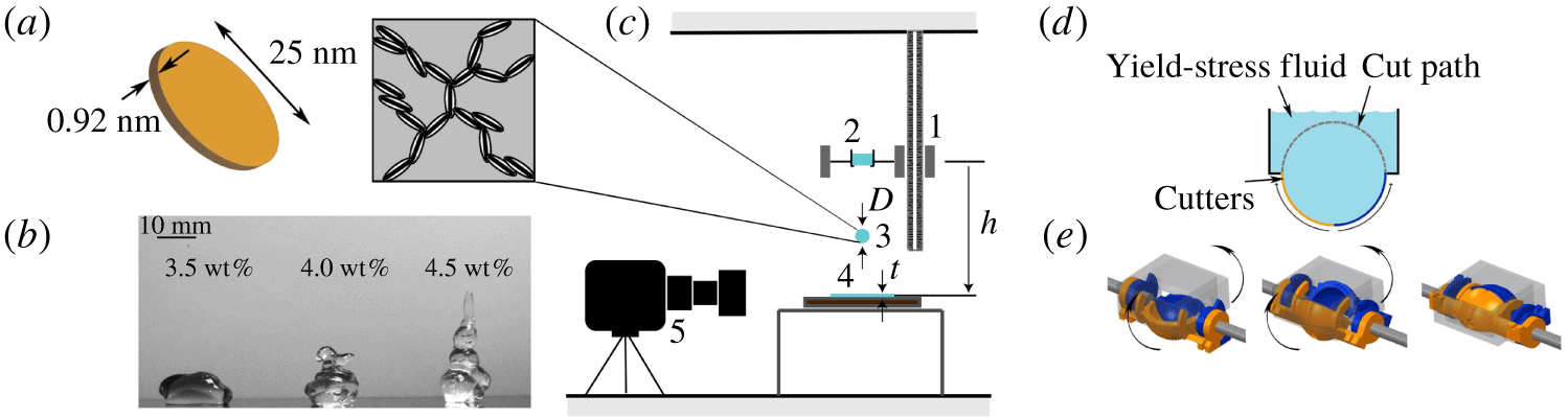
Experimental set-up. (a) Structure of Laponite clay particles, with disc-like particles stacked in suspension (image adapted from Tanaka, Meunier & Bonn (Reference Tanaka, Meunier and Bonn2004), reused with permission). (b) The yield stress of Laponite helps it retain its shape against gravity and this becomes more prominent as the concentration increases from 3.5 through 4.5 wt %. (c) Schematic of drop impact set-up. The geometric parameters: drop diameter,  $D$, coating thickness,
 $t$, drop height,
 $h$, are labelled. The components are as follows: 1, variable height trolley; 2, drop maker with fluid; 3, discharged drop; 4, fluid coating on substrate; 5, high-speed camera. (d) The schematic of the drop maker and the side view of how the spherical shape is formed. (e) Three-dimensional model of the device in starting, intermediate and final positions (left-to-right). (d,e) Adapted from Blackwell et al. (Reference Blackwell, Deetjen, Gaudio and Ewoldt2015).

2 Materials and methods
2.1 Drop impact set-up
Figure 1 outlines the experimental set-up. The experimental parameters varied were as follows: impact velocity,  $V$; drop diameter,
 $D$; coating thickness,
 $t$; and concentration,
 $c$. The ranges of values for each are shown in table 1. The range of values for the fluid properties
 $\unicode[STIX]{x1D70E}_{y}$ (shear yield stress),
 $K$ (consistency index) and
 $\unicode[STIX]{x1D702}_{\infty }$ (infinite shear viscosity) are obtained from the range of concentrations used and the corresponding generalised Herschel–Bulkley model fits in figure 2(a). The significant change in
 $\unicode[STIX]{x1D70E}_{y}$ is shown in figure 1(b). To achieve reproducibility and correctness of measurement, spherical drops must be used in the tests. For this, as shown in figure 1(d,e), a drop chopper mechanism designed by Blackwell et al. was used (Blackwell et al. Reference Blackwell, Deetjen, Gaudio and Ewoldt2015). It consists of a pair of 3D printed counter-rotating acrylic hemispheres. These were coated on the inside to make them hydrophobic so that the water-based gels would detach easily. The diameter of the hemispheres is changed to obtain the desired drop diameter. This was used to dispense approximately spherical drops onto the substrate coated with the Laponite suspension. The coating was of the same material as that of the impacting drop. Properties of the substrate underneath the fluid film can be important, especially for drop impact of yield-stress fluids on dry substrates and thin films because these fluids might slip at a solid surface (Kalyon Reference Kalyon2005; Jalaal, Balmforth & Stoeber Reference Jalaal, Balmforth and Stoeber2015; Bonn et al. Reference Bonn, Denn, Berthier, Divoux and Manneville2017), especially rough and hydrophobic surfaces (Luu & Forterre Reference Luu and Forterre2013). In our experiments we use a smooth hydrophilic Pyrex™ glass plate as the substrate, which has a mean surface roughness,
 $R_{a}\sim 1~\unicode[STIX]{x03BC}\text{m}$ (Preedy et al. Reference Preedy, Perni, Nipiĉ, Bohinc and Prokopovich2014). We observe no obvious slip in our experiment, but a systematic study of this is outside the scope of our study here. A high-speed camera (Photron Fastcam Mini UX-100) was used to capture the impact event at 4000 frames per second. Standard backlit videos were recorded to capture the drop event, where the fluid appears dark and very well contrasted against a bright white background. Drops fell onto the coated glass substrate (fluid coating thickness,
 $t$), from a specific height,
 $h$, controlled by the movable trolley upon which the drop maker device was mounted, to achieve the desired impact velocity,
 $V$ (figure 1c). The effect of air drag has been neglected in the calculation of
 $V$ based on
 $h$, and has been verified to be a very good approximation by tracking the velocity of the impacting drop from the videos (Tracker Video Analysis and Modeling Tool, the free video tracking software used). The observed velocities were well within 5 % of the theoretical value in the absence of air resistance, the free-fall velocity of
 $\sqrt{2gh}$, where
 $g$ is the acceleration due to gravity. The velocity
 $V=\sqrt{2gh}$ is used in our calculations.
The velocities tested (by varying the trolley height  $h$) were
 $V=2.0$, 2.4, 3.0, 3.6, 4.0, 4.5, 5.0 and
 $6.0~\text{m}~\text{s}^{-1}$. The film thicknesses used were
 $t=0.25$, 0.5, 1.0, 1.5, 2.1, 2.9 and 3.2 mm. Three drop maker diameters,
 $D=10$, 15 and 20 mm, were used. The flow properties of Laponite are listed in table 1. For each combination of parameters, duplicate tests were done for repeatability, which amounted to testing 504 different test conditions, each tested twice, resulting in 1008 separate drop impact tests performed. After each test, the fluid in the coating was replaced with a freshly stirred sample, identical to the one loaded on the drop maker, and the tests conducted within a 10 s window.
Range of experimental (geometric and material) parameters explored, with rheological parameters corresponding to the fits to the generalised Herschel–Bulkley model with  $n=0.5$. The ranges of the quantities
 $\unicode[STIX]{x1D70E}_{y}$,
 $K$ and
 $\unicode[STIX]{x1D702}_{\infty }$ are determined by the range of weight fractions of Laponite tested, which were 3.5, 4.0 and 4.5 wt %.

2.2 Materials
Laponite (figure 1a,b) is a crystalline powder of colloidal discs composed of lithium sodium magnesium silicate ( $\text{Na}_{0.7}^{+}[\text{Si}_{8}\text{Mg}_{5.5}\text{Li}_{0.3}\text{O}_{20}(\text{OH})_{4}]_{0.7}^{-}$), and forms a soft gel when dispersed in aqueous solution. The platelet-shaped particles are approximately 25 nm in diameter and 0.92 nm thick (Cummins Reference Cummins2007). The faces of the discs are negatively charged, and, depending on the pH of the solution, the sides can hold partial positive charge (Bonn et al. Reference Bonn, Kellay, Tanaka, Wegdam and Meunier1999). Due to this, attractive forces exist between the discs and they come together to form a stacked house of cards structure (Bonn et al. Reference Bonn, Kellay, Tanaka, Wegdam and Meunier1999; Tanaka et al. Reference Tanaka, Meunier and Bonn2004; Cummins Reference Cummins2007) (figure 1a). The suspensions used in the experiments were prepared by dissolving required amounts of Laponite RD powder (Conservation Support Systems, USA) in water to achieve the desired weight fraction. The powder was dissolved in water in a laboratory magnetic stirrer, sealed to prevent evaporation of the suspending medium and left to stir for 3 days. Mass densities of Laponite suspensions were determined by weighing known volumes of the fluid, and all samples had densities close to that of pure water,
 $\unicode[STIX]{x1D70C}=1000~\text{kg}~\text{m}^{-3}$. This fiducial value was thus used in the dimensionless group as well. Prior to testing, the samples were subjected to stirring in a laboratory impeller mixer at 300 r.p.m. for 2 minutes. The samples were tested within 10 s of the stirring to minimise any thixotropic restructuring (most clays are thixotropic, but this is not a focus of this work) (Mewis Reference Mewis1979; Mewis & Wagner Reference Mewis and Wagner2009).
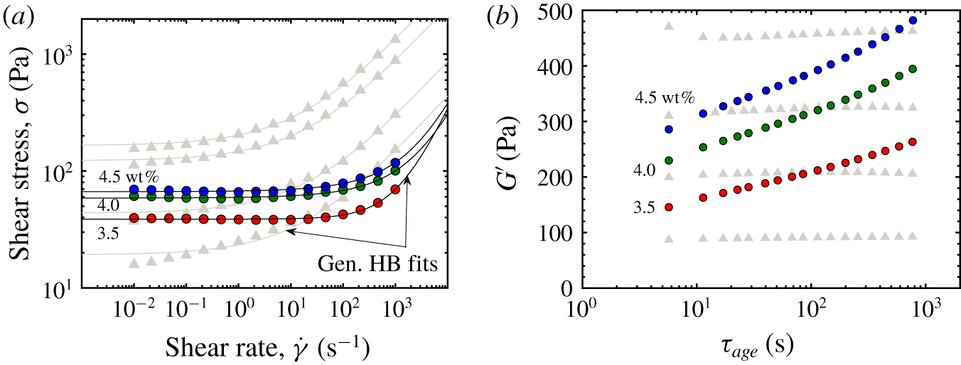
Rheological characterisation of Laponite (dark, coloured symbols) compared to Carbopol (grey symbols). Carbopol concentrations shown here match those used in Blackwell et al. (Reference Blackwell, Deetjen, Gaudio and Ewoldt2015). (a) Steady-state flow curves with fits to the generalised Herschel–Bulkley model with  $n=0.5$ (2.4), giving the parameters
 $\unicode[STIX]{x1D70E}_{y}$,
 $K$ and
 $\unicode[STIX]{x1D702}_{\infty }$. (b) Thixotropic stress recovery (aging at rest) of the storage modulus
 $G^{\prime }$. The increase of
 $G^{\prime }$ is significant for Laponite (nearly doubles for each concentration), but our experiments are conducted within a 10 s window, so we are within the earliest stages and consider our materials ‘unaged’. Carbopol does not show appreciable thixotropic aging for the time scales shown.

Carbopol is used for comparison as a yield-stress fluid. It is a soft, jammed, ‘glassy’ (repulsion dominated) fluid, in contrast with Laponite which is a ‘gel’ (attraction dominated) fluid (Nelson & Ewoldt Reference Nelson and Ewoldt2017). Carbopol (generic name carbomer) particles are made of cross-linked poly(acrylic acid). Upon dispersion in water, this forms a viscous suspension with  $\text{pH}\approx 4$, and particles start swelling with the solvent. Upon neutralisation with a base, the soft particles acquire negative charges by losing protons, and swell further. The swollen particles repel each other by virtue of their like charges and steric interactions. Around
 $\text{pH}\approx 7$, the particles reach maximum swelling and get jammed, forming a soft glassy fluid (Piau Reference Piau2007; Nelson & Ewoldt Reference Nelson and Ewoldt2017). Increasing the pH further collapses the particles and the viscosity and yield stress decrease drastically. Carbopol glasses were prepared by thoroughly mixing the powder form (Carbopol 940, Lubrizol) in water overnight using a magnetic stirrer at 300 r.p.m. After mixing, 1 N aqueous NaOH solution was added drop by drop until the pH was stable around
 $7\pm 0.25$. The neutralised Carbopol formulations were stirred overnight at 200 r.p.m. to homogeneously disperse the particles with the base and remove any air bubbles. Samples were then tested for rheological properties, both in steady shear and thixotropic characterisation, with the steady shear data similar to those in Blackwell et al. (Reference Blackwell, Deetjen, Gaudio and Ewoldt2015). No drop impact tests were done here, and we use drop impact results for Carbopol adapted from Blackwell et al. (Reference Blackwell, Deetjen, Gaudio and Ewoldt2015) to only compare with the results newly obtained here with Laponite.
We assume that the surface tension of all Laponite formulations is approximately the same, and not much different from that of water, approximately (this is the same fiducial value assumed for Carbopol in Jalaal et al. (Reference Jalaal, Kemper and Lohse2019)). Measurement of surface tension in yield-stress fluids is extremely difficult. We did not make any measurements for the surface tension of Laponite, but published results for aqueous Carbopol suspensions indicate surface tension values less than 10 % lower than water (Manglik, Wasekar & Zhang Reference Manglik, Wasekar and Zhang2001; Jørgensen et al. Reference Jørgensen, Le Merrer, Delanoë-Ayari and Barentin2015).
2.3 Rheological characterisation of Laponite
Rheological characterisation of Laponite samples included steady shear flow curves and thixotropic recovery tests (figure 2). The steady shear flow data for Laponite were taken on a DHR-3 stress-controlled rheometer, TA Instruments. We used a parallel-plate geometry, 20 mm in diameter, with the rate ramp going from the highest  $(1000~\text{s}^{-1})$ to the lowest rate
 $(0.01~\text{s}^{-1})$. The yield stress
 $\unicode[STIX]{x1D70E}_{y}$ obtained is the dynamic shear yield stress, and is relevant for the unaged samples. Samples were tested at different gaps of
 $400$ and
 $600~\unicode[STIX]{x03BC}\text{m}$ (full data shown in supplementary information, section 1 available at https://doi.org/10.1017/jfm.2020.147) to check for slip and a less than 10 % difference between the two sets of data was found. All tests were conducted at a constant temperature of
 $25\,^{\circ }\text{C}$. Identical procedures were followed in taking steady shear data for Carbopol.
Thixotropic recovery data for Laponite are shown in figure 2(b). The existence of a particulate network inside the solvent renders a structure to the Laponite suspension. Upon shearing from a rest state (or stepping up to a higher shear rate than the original), this structure (or flocs in many cases for colloids) can break down over time, and consequently the viscosity of the material decreases. The structure can build up again upon cessation of shear (or stepping down to a lower shear rate). This spontaneous breakdown and build up of structure over time when subjected to varying shear histories is called thixotropy (Mewis Reference Mewis1979; Mewis & Wagner Reference Mewis and Wagner2009). Since a suspension of Laponite in water is noticeably thixotropic (figure 2b), here, we carefully conduct drop impact tests before the structure recovers or ages significantly. This is required to truly test unaged (also known as rejuvenated) samples, and hence negate the effect of thixotropic aging, which can play a major role in drop impact dynamics by changing the material properties and introducing anisotropy. Such effects can break down scaling relations, as has been acknowledged by Luu & Forterre (Reference Luu and Forterre2009). In figure 2(b), the recovery of the structure of Laponite has been shown by monitoring the viscoelastic storage modulus,  $G^{\prime }(\unicode[STIX]{x1D714})$ (at a fixed frequency,
 $\unicode[STIX]{x1D714}=10~\text{rad}~\text{s}^{-1}$, and oscillation strain amplitude,
 $\hat{\unicode[STIX]{x1D6FE}}=1\,\%$), over time of aging,
 $\unicode[STIX]{x1D70F}_{age}$. The value of
 $\unicode[STIX]{x1D70F}_{age}$ is measured from the point of cessation of a pre-shear applied to the samples at
 $\dot{\unicode[STIX]{x1D6FE}}=100~\text{s}^{-1}$ for 2 min. All oscillatory tests were conducted on an ARES-G2 rheometer, TA Instruments, which is a strain-controlled, separated motor-transducer rheometer. An Advanced Peltier System (APS) was used to maintain the temperature during the tests at
 $25\,^{\circ }\text{C}$ and 25 mm parallel plates were used at two different gaps (1000 and
 $1250~\unicode[STIX]{x03BC}\text{m}$) to verify the absence of slip. Less than 5 % difference between the data sets was observed. Drop impact tests were conducted within a 10 s window after stirring. Since the sample does not recover significantly within 10 s, thixotropic effects can be neglected. Aging data were taken for Carbopol and have been co-plotted in the background. This observation matches with those in Blackwell et al. (Reference Blackwell, Deetjen, Gaudio and Ewoldt2015), where effects of thixotropic aging were neglected. Since thixotropic aging is neglected in our drop impact tests, the steady shear flow data in figure 2(a) are used to understand the results and define dimensionless groups, as in (1.2c).
Steady-state rheological data, as in figure 2(a), are usually fit to what are known as generalised Newtonian fluid (GNF) models which are of the form
 $$\begin{eqnarray}\text{}\underline{\text{}\underline{\unicode[STIX]{x1D70E}}}=\unicode[STIX]{x1D702}(\dot{\unicode[STIX]{x1D6FE}};\unicode[STIX]{x1D703}_{i})\text{}\underline{\text{}\underline{\dot{\unicode[STIX]{x1D6FE}}}},\end{eqnarray}$$
where  $\text{}\underline{\text{}\underline{\unicode[STIX]{x1D70E}}}$ is the stress tensor, and the viscosity,
 $\unicode[STIX]{x1D702}$, is a function of a characteristic strain rate,
 $\dot{\unicode[STIX]{x1D6FE}}$, which is defined from the second invariant of the rate of deformation tensor,
 $\text{}\underline{\text{}\underline{\dot{\unicode[STIX]{x1D6FE}}}}=\text{}\underline{\unicode[STIX]{x1D735}}\,\text{}\underline{v}+(\text{}\underline{\unicode[STIX]{x1D735}}\,\text{}\underline{v})^{T}$, as
 $\dot{\unicode[STIX]{x1D6FE}}=\sqrt{\frac{1}{2}\text{}\underline{\text{}\underline{\dot{\unicode[STIX]{x1D6FE}}}}:\text{}\underline{\text{}\underline{\dot{\unicode[STIX]{x1D6FE}}}}}$ (Bird et al. Reference Bird, Armstrong and Hassager1987; Nguyen & Boger Reference Nguyen and Boger1992; Macosko Reference Macosko1994; Balmforth et al. Reference Balmforth, Frigaard and Ovarlez2014; Coussot Reference Coussot2014; Bonn et al. Reference Bonn, Denn, Berthier, Divoux and Manneville2017). For simple shearing flows, this is given by the shear rate measured by the instrument. The functional form usually involves other parameters,
 $\unicode[STIX]{x1D703}_{i}$, which are characteristic of the fluid tested. Many such GNF models exist, and the simplest of the viscoplastic models is the Bingham model (Bird et al. Reference Bird, Armstrong and Hassager1987; Macosko Reference Macosko1994), which is given in one-dimensional steady shear as
 $$\begin{eqnarray}\unicode[STIX]{x1D70E}=\unicode[STIX]{x1D70E}_{y}+\unicode[STIX]{x1D702}_{\infty }\dot{\unicode[STIX]{x1D6FE}}\equiv \left(\frac{\unicode[STIX]{x1D70E}_{y}}{\dot{\unicode[STIX]{x1D6FE}}}+\unicode[STIX]{x1D702}_{\infty }\right)\dot{\unicode[STIX]{x1D6FE}},\end{eqnarray}$$
where  $\unicode[STIX]{x1D70E}$ is the shear stress. The viscosity is then defined as
 $\unicode[STIX]{x1D702}\equiv \unicode[STIX]{x1D70E}/\dot{\unicode[STIX]{x1D6FE}}$. The above form is applicable when
 $\unicode[STIX]{x1D70E}\geqslant \unicode[STIX]{x1D70E}_{y}$. When
 $\unicode[STIX]{x1D70E}<\unicode[STIX]{x1D70E}_{y}$, there is no flow, and
 $\dot{\unicode[STIX]{x1D6FE}}=0$. These are true of all viscoplastic models. The model parameters
 $\unicode[STIX]{x1D70E}_{y}$ and
 $\unicode[STIX]{x1D702}_{\infty }$ are the yield stress and the infinite-shear viscosity respectively for the material. A more complex model can fit better, such as the Herschel–Bulkley (HB) model (Bird et al. Reference Bird, Armstrong and Hassager1987; Macosko Reference Macosko1994; Nelson & Ewoldt Reference Nelson and Ewoldt2017), given by
 $$\begin{eqnarray}\unicode[STIX]{x1D70E}=\unicode[STIX]{x1D70E}_{y}+K\dot{\unicode[STIX]{x1D6FE}}^{n}\equiv \unicode[STIX]{x1D70E}_{y}\left[1+\left(\frac{\dot{\unicode[STIX]{x1D6FE}}}{\dot{\unicode[STIX]{x1D6FE}}_{crit}}\right)^{n}\right].\end{eqnarray}$$
Here, we still have the same  $\unicode[STIX]{x1D70E}_{y}$ parameter, but
 $\unicode[STIX]{x1D702}_{\infty }$ is replaced by
 $K$, called the consistency index, and an additional parameter
 $n$, called the flow index. An equivalent, but better form of the model is also shown, which involves a critical shear rate,
 $\dot{\unicode[STIX]{x1D6FE}}_{crit}$, instead of
 $K$ as a parameter (Nelson & Ewoldt Reference Nelson and Ewoldt2017) since the dimensions of
 $K$ are variable, depending on the value of
 $n$. The Bingham model has a finite viscosity at very high shear rates, a more physical behaviour than the HB model, for which the viscosity vanishes (when
 $n<1$). Therefore, we can also fit the rheological data in figure 2(a) to a generalised Herschel–Bulkley model, given by
 $$\begin{eqnarray}\unicode[STIX]{x1D70E}=\unicode[STIX]{x1D70E}_{y}+K\dot{\unicode[STIX]{x1D6FE}}^{n}+\unicode[STIX]{x1D702}_{\infty }\dot{\unicode[STIX]{x1D6FE}},\end{eqnarray}$$
and this retains the high-rate scaling of the Bingham model, while fitting rheological data well for most gels and colloids, as is the case with the HB model. Note that this model has four free parameters. One may not have enough data points in steady flow to give accurate estimates of each parameter, which can then have large fit uncertainties. To tackle this, we have fit our data to a particular case of this model, one for which  $n$ is held fixed at 0.5, while the other three parameters,
 $\unicode[STIX]{x1D70E}_{y}$,
 $K$ and
 $\unicode[STIX]{x1D702}_{\infty }$, are free. This assumption is in agreement with the literature on soft-particle glasses and particulate gels where this Herschel–Bulkley scaling exponent,
 $n$, is found to be close to 0.5 (Cloitre et al. Reference Cloitre, Borrega, Monti and Leibler2003; Bécu, Manneville & Colin Reference Bécu, Manneville and Colin2006; Denkov et al. Reference Denkov, Tcholakova, Golemanov, Ananthapadmanabhan and Lips2008; Nordstrom et al. Reference Nordstrom, Verneuil, Arratia, Basu, Zhang, Yodh, Gollub and Durian2010; Seth et al. Reference Seth, Mohan, Locatelli-Champagne, Cloitre and Bonnecaze2011; Paredes, Michels & Bonn Reference Paredes, Michels and Bonn2013; Basu et al. Reference Basu, Xu, Still, Arratia, Zhang, Nordstrom, Rieser, Gollub, Durian and Yodh2014; Pellet & Cloitre Reference Pellet and Cloitre2016). We use this model to fit our data, with the resulting fit parameters used to compute dimensionless groups for plotting the regime maps.
For the sake of completeness, we fit the steady shear data to all three models: Bingham, generalised Herschel–Bulkley with  $n=0.5$ and the full generalised Herschel–Bulkley. We then carry out an approximate Bayesian analysis that provides a metric to find the most credible model: one where a model is penalised for using excessive parameters. This analysis gives the generalised Herschel–Bulkley with
 $n=0.5$ to be the most credible model for Carbopol, while it is the second best for Laponite. This supports our rationale for using this model to re-frame the original dimensionless group that used the Bingham model. Full details can be found in the supplementary information (section 1).
3 Results of drop impacts
3.1 Drop impact events and related phenomenology
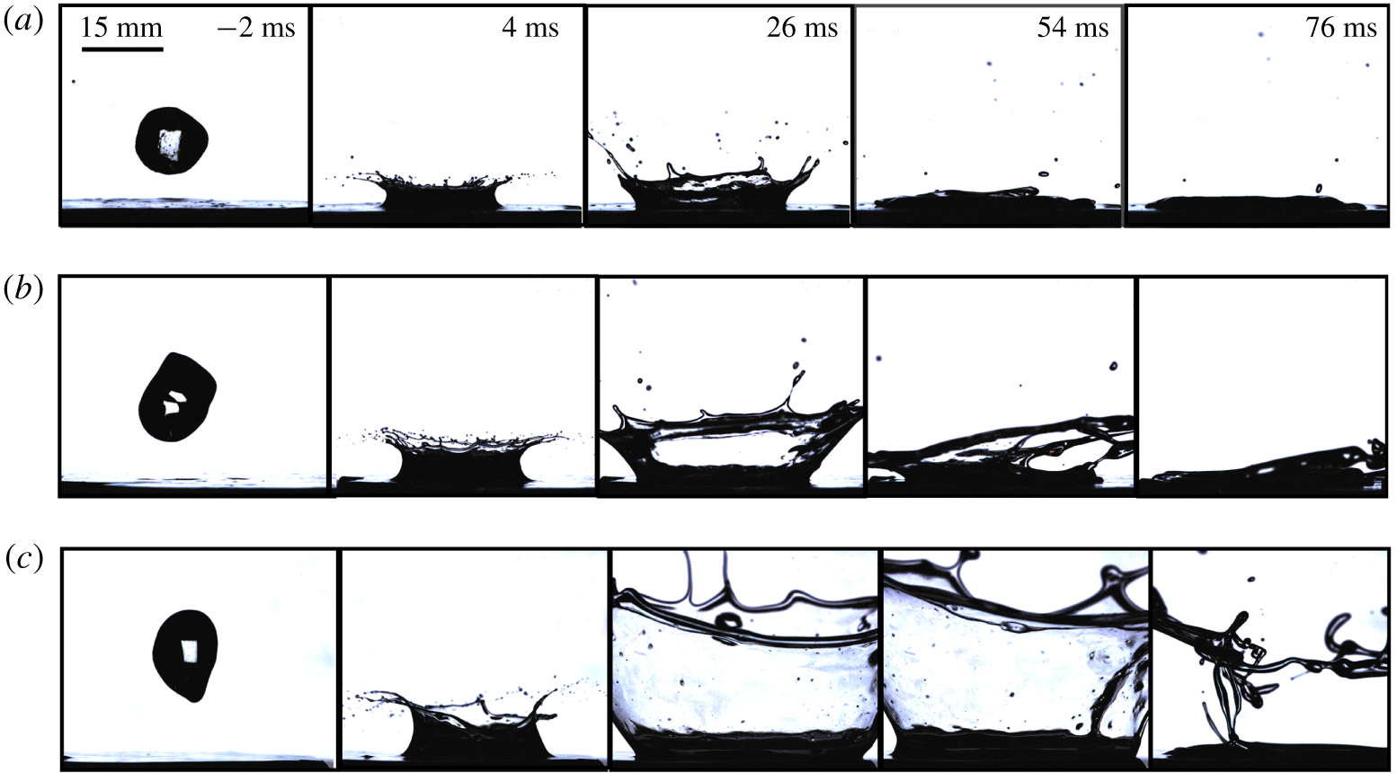
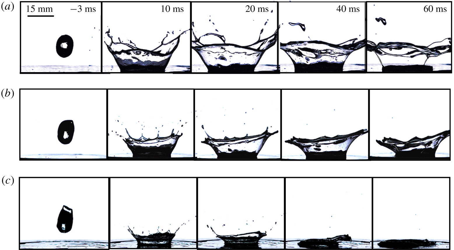
Figure 3 shows representative impact results from among the 504 different cases tested. The results of the impact tests are shown via the screenshots from the videos at key instances of time. It shows a comparison between three different velocities while the other parameters (concentration,  $c$, drop diameter,
 $D$, and coating thickness,
 $t$) were held constant (we show several additional representative results for the effect of varying each of the four parameters in appendix A). Note that the time
 $\unicode[STIX]{x1D70F}=0$ is taken at the instant of impact, so the first tile in each row is shown in negative time relative to the impact frame, which happens at
 $\unicode[STIX]{x1D70F}=0$. Time evolves towards positive as we move forward with the impact. As we move from an impact velocity of 2.4 to 3.0 to 3.6 m
 $\hspace{2.22198pt}$s
 $^{-1}$, the impact event involves more splash and ejection of fluid away from the impact site; this can be detected by either looking at the height of the top of the ejection sheet crown from its base, or at the diameter of the impact crater formed in the coating itself.
Effect of varying impact velocities. Drops of  $D=15~\text{mm}$, 3.5 wt % Laponite impacting a
 $t=2.9~\text{mm}$ thick coating of correspondingly the same material at (a)
 $V=2.4$, (b)
 $3.0$ and (c)
 $3.6~\text{m}~\text{s}^{-1}$. For the same experimental conditions, samples splash more as the impact velocity is increased, which is expected, since the inertial forces, which are responsible for promoting splash, increase with velocity.

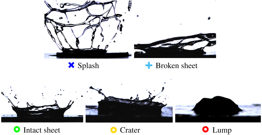
The type of impact and ejection event is classified as one of five different regimes as shown in figure 4, following the convention in Blackwell et al. (Reference Blackwell, Deetjen, Gaudio and Ewoldt2015). The exact details shall not be repeated here. These typical impact events represent all possible impact behaviours in our tests when a viscoplastic drop hits a viscoplastic fluid film. The first two types, called a splash and a broken sheet, are classified as ‘splash’-type behaviours, and the last three, called intact sheet, crater and lump, are the ‘stick’-type behaviours. Note that we observe the so-called ‘prompt’ splash in almost all impact events. What we choose to broadly call a ‘splash’-type behaviour is typically referred to as a ‘delayed’ splash in the literature. So we look for a delayed rupture of the ejecta sheet, which happens well beyond the prompt splash that happens immediately upon impact. Very little variation in impact result type is observed between duplicates. For the very few cases where there is a variation, which always occurred near the boundary between two impact types, we forced it to be of the more ‘splash’ type of the two. Since there might have been some variability in the time within which the test was conducted, and the Laponite could have aged as a result, it is safe to assume the impact would have been more ‘splash’ than ‘stick’ if the sample had not aged.
Using this classification, we can determine the impact types for each event in figure 3. In (a), we observe an ejection sheet in the frame at  $+26~\text{ms}$, which then collapses, but remains intact. This is an intact sheet. In (b), the ejection sheet is again formed at
 $+26~\text{ms}$, but this breaks up in the subsequent frame at
 $+54~\text{ms}$, which then collapses, and hence this is a broken sheet. In (c), a large ejection sheet is formed compared to the two earlier velocities, and this keeps expanding until eventually rupturing into many fragments, as seen in the frame at
 $+76~\text{ms}$. This is called a ‘splash’. Note that the stickier the event, the faster it reaches completion in that the kinetic energy is dissipated more quickly. So, as we move from (a) to (c), the event completion is delayed further and further. For (c), the ruptured sheet has not even collapsed completely in the final frame shown.
Various impact events observed during experiments. The first two types, splash and broken sheet, are labelled as ‘splashy’ behaviours, while the last three types, intact sheet, crater and lump, are called the ‘sticky’-type behaviours. The impact event types shown here are used as references for judging the type of impact, and the legends used here are consistent with those used in the regime maps that follow. See also supplementary movie 1.

3.2 Dimensionless numbers and impact regimes
We use the classification scheme (figure 4) to assign a category to each of the observed impacts, allowing us to make regime maps (figure 5). The symbols shown in figure 4 beneath each impact type are used to code the impact regime maps, with each point corresponding to a specific experimental configuration which is represented by the  $y$ and
 $x$ coordinates (which correspond to the specific values of experimental parameters
 $V$,
 $D$,
 $t$ and
 $c$). To collapse multi-dimensional data into a two-dimensional (2-D) plot, we need to use a scaling law or a dimensionless grouping.
The hypothesis here (Blackwell et al. Reference Blackwell, Deetjen, Gaudio and Ewoldt2015) is much stronger than a basic dimensional analysis. It is based on a force-balance argument that takes into account the competing effects of inertial and flow forces, while ignoring other effects such as surface tension and gravity in comparison to these. We use the Buckingham- $\unicode[STIX]{x1D6F1}$ theorem to elucidate this. The system has three experimental parameters, velocity
 $V$, drop diameter
 $D$ and thickness
 $t$, along with gravity,
 $g$, and two fluid properties, density
 $\unicode[STIX]{x1D70C}$ and surface tension
 $\unicode[STIX]{x1D6FE}$, in addition to at least four rheological properties, yield-stress
 $\unicode[STIX]{x1D70E}_{y}$, consistency index
 $K$, flow index
 $n$ and Bingham plastic viscosity
 $\unicode[STIX]{x1D702}_{\infty }$. This comes to a total of 10 parameters. So the splash type behaviour can be thought of as a function of these, written as
 $$\begin{eqnarray}\text{splash type}=f(V,D,t,g,\unicode[STIX]{x1D70C},\unicode[STIX]{x1D6FE};\unicode[STIX]{x1D70E}_{y},K,n,\unicode[STIX]{x1D702}_{\infty }).\end{eqnarray}$$
Since  $n$ is an exponent, it is already dimensionless. Including
 $n$, we thus get the number of parameters as
 $A=10$. The dimensions in the problem involve all three, mass
 $[M]$, length
 $[L]$ and time
 $[T]$, and so
 $B=3$. From the Buckingham-
 $\unicode[STIX]{x1D6F1}$ theorem, one needs at most
 $A-B=7$ dimensionless groups to describe the system fully. These are the generalised Reynolds,
 $Re=\unicode[STIX]{x1D70C}V^{2}/(\unicode[STIX]{x1D70E}_{y}+K(V/t)^{n}+\unicode[STIX]{x1D702}_{\infty }V/t)$, Bingham,
 $Bn=\unicode[STIX]{x1D70E}_{y}/(K(V/t)^{n}+\unicode[STIX]{x1D702}_{\infty }V/t)$, generalised capillary,
 $Ca=(\unicode[STIX]{x1D70E}_{y}+K(V/t)^{n}+\unicode[STIX]{x1D702}_{\infty }V/t)/\unicode[STIX]{x1D6FE}/D$ and Froude,
 $Fr=V/\sqrt{gD}$, numbers, along with a dimensionless consistency index,
 $K^{\ast }=K(V/t)^{n}/(\unicode[STIX]{x1D70E}_{y}+K(V/t)^{n}+\unicode[STIX]{x1D702}_{\infty }V/t)$, the exponent
 $n$, and the dimensionless coating thickness,
 $t/D$ (Thompson & Soares Reference Thompson and Soares2016). Weber number is not an independent group, since it can be written as
 $We=(\unicode[STIX]{x1D70C}V^{2}D)/\unicode[STIX]{x1D6FE}=Re\,Ca$. Note that the plastic number,
 $Pl=\unicode[STIX]{x1D70E}_{y}/(\unicode[STIX]{x1D70E}_{y}+K(V/t)^{n}+\unicode[STIX]{x1D702}_{\infty }V/t)$, is not separate, since
 $Pl=Bn/(1+Bn)$. Now, if we neglect the effect of surface tension when compared to flow stresses,
 $Ca$ can be neglected since it is very large;
 $Ca$ also encompasses the dimensionless group
 ${\mathcal{Y}}=\unicode[STIX]{x1D70E}_{y}/(\unicode[STIX]{x1D6FE}/L)$, comparing plastic and capillary stresses, where
 $L$ is a characteristic length scale related to capillary pressure (German & Bertola Reference German and Bertola2010; Jalaal et al. Reference Jalaal, Kemper and Lohse2019). If we set
 ${\mathcal{Y}}=1$ , we can estimate a characteristic length scale below which surface tension effects dominate the yield stress,
 $L_{c}=\unicode[STIX]{x1D6FE}/\unicode[STIX]{x1D70E}_{y}$. For the range of yield stress for the Laponite suspensions, 40–70 Pa, and an upper-bound estimate of surface tension,
 $70~\text{mN}~\text{m}$, this results in a critical length scale ranging from 1.8–1.0 mm, respectively. Below this length scale, surface tension may be important. Our film thicknesses are of this order, but are flat (no curvature) and therefore are stable. Our drop sizes are all larger, and are also stabilised by the yield stress. But droplet breakup does seem to occur at or below these length scales as observed in the video frames where ejected droplets have length scales of this size or smaller. Using the full
 $Ca$ gives even smaller values of
 $L_{c}$.
Similar scaling holds for the Froude number since the drop diameter is much smaller than the velocity (inertial) scale;  $Re,Bn,K^{\ast }$ and
 $t/D$, combine to capture the remaining effects of inertia, viscosity and plasticity. These can be collapsed into a single dimensionless group using a simple force-balance argument, such that
 $$\begin{eqnarray}\frac{\text{inertial forces}}{\text{flow forces}}\sim \frac{\unicode[STIX]{x1D70C}V^{2}(D^{2})}{[\unicode[STIX]{x1D70E}_{y}+K(V/t)^{n}+\unicode[STIX]{x1D702}_{\infty }V/t](Dt)}\equiv \text{IF}\left(\frac{D}{t}\right).\end{eqnarray}$$
This group compares the inertial forces (responsible for drop breakup or ‘splash’) to the dissipative flow forces (responsible for dissipating the energy and promoting ‘stick’ behaviours). The numerator is the inertial force term, where  $\unicode[STIX]{x1D70C}$ is the fluid density,
 $V$ is the impact velocity and
 $D$ is the impacting drop diameter. The denominator is the flow forces term, where
 $\unicode[STIX]{x1D70E}_{y}$ is the yield stress,
 $K$ is the consistency index,
 $n$ is the flow index,
 $\unicode[STIX]{x1D702}_{\infty }$ is the infinite-shear viscosity and
 $t$ is the coating thickness. As mentioned earlier, we use
 $n=0.5$ throughout. We will test if this group (i) is capable of distinguishing impact regimes for Laponite, (ii) provides a constant critical value of (1.2c) for Laponite and (iii) gives different critical values for Laponite versus Carbopol.
From the definition, we see that this non-dimensionalisation is reminiscent of the classical Reynolds number, except that this is different because the retarding force is not just viscous (rate dependent); it is a combination of a yield stress and a viscosity. Nevertheless, this group reduces to a Reynolds number in the limit of a Newtonian fluid for which  $\unicode[STIX]{x1D70E}_{y}=0$, and the viscosity would be a constant,
 $\unicode[STIX]{x1D702}_{\infty }+K=\unicode[STIX]{x1D707}$ with
 $n=1$. This scaling introduced in Blackwell et al. (Reference Blackwell, Deetjen, Gaudio and Ewoldt2015) has thus been referred to as a modified Reynolds number in the literature (Thompson & Soares Reference Thompson and Soares2016; Jalaal et al. Reference Jalaal, Kemper and Lohse2019). The expression in (3.2) can be simplified by defining a ratio of stresses, IF, as in (1.2c).
Here, we hypothesise a critical value of this ratio,  $C$, above which inertial forces dominate and below which flow forces govern the behaviour. Consequently, we use
 $C$ to define the regime boundary between stick and splash impact types,
 $$\begin{eqnarray}\frac{\unicode[STIX]{x1D70C}V^{2}}{\unicode[STIX]{x1D70E}_{y}+K(V/t)^{0.5}+\unicode[STIX]{x1D702}_{\infty }V/t}\left(\frac{D}{t}\right)\approx C.\end{eqnarray}$$
One can treat the parameter  $C$ as a critical number above which splashing behaviours are observed, while values less than
 $C$ give one of the three stick-type behaviours. The exact numerical value of
 $C$ depends on which boundary between impact regimes is chosen to be suggestive of the transition between stick to splash behaviour. We elaborate further on this aspect when we discuss the specific regime maps for our data.
We hypothesise that, to leading order, the only forces or stresses dominating the impact event are inertial and flow (viscous); other contributions due to extensibility, thixotropy, chemical structure and morphology, surface tension etc. are neglected within the range of conditions tested. The values of the Bond number ( $Bo$, comparing gravity with surface tension), the Weber number (
 $We$, comparing inertia with surface tension) and the capillary number (
 $Ca$, comparing viscous forces with surface tension) are very large for our test conditions, so surface tension can be neglected compared to viscous and inertial effects. As a consequence, the only properties that matter are rheological, and specifically the steady-state flow properties of the material are used, and hence the form shown in (1.2c) is employed. The scaling might fail for materials or flows where these effects (surface tension, extensibility, thixotropy, viscoelastic transient behaviour, etc.) cannot be neglected, but we show that for our system and range of test conditions, the forces considered (inertia and flow) are sufficient to capture the leading-order physics.
In Blackwell et al. (Reference Blackwell, Deetjen, Gaudio and Ewoldt2015), for Carbopol, IF was plotted versus  $t/D$, and the regime boundary was observed to be of an approximately constant slope of 1 (Blackwell et al. Reference Blackwell, Deetjen, Gaudio and Ewoldt2015). Here, we plot IF
 $(D/t)$ versus
 $t/D$ instead. If our hypothesis holds, the regime boundary should now appear as a line with zero slope. The
 $y$-coordinate of this horizontal line separating two regimes of choice should give the critical value of (1.2c), which we call
 $C$. The value of
 $C$ is determined from the regime maps, details of which are provided in appendix B. Note that we restrict the values of
 $t/D$ to be greater than 0.1 while finding the value of
 $C$. We do this because the data set is sparse for the lower ranges of
 $t/D$, and reliable estimates of a regime boundary cannot be obtained. Full plots are shown in the supplementary information (§ 8). Once we obtain the value of
 $C$ for each map, we hypothesise that we will get a ‘splash’ event when
 $$\begin{eqnarray}\text{IF}\left(\frac{D}{t}\right)\gtrsim C.\end{eqnarray}$$
We assume in this non-dimensionalisation that the thickness of the coating,  $t$, is the sole length scale relevant to calculate the shear rates during impact. The ejection sheet and surrounding medium (here, air) do not have any influence on the results. This helps keep the non-dimensionalisation simple. This is not expected to work universally, for instance, when the coating is too thin (
 $t\approx 0$) or is a pool of fluid instead of a thin film (behaves like a semi-infinite medium,
 $t\rightarrow \infty$). The range of relative thickness (normalised by drop diameter,
 $t/D$) that we explore is neither of these two extreme cases.
Regime maps for unaged Laponite. (a) 3.5 wt % ( $\unicode[STIX]{x1D70E}_{y}=40~\text{Pa}$,
 $K=0.04~\text{Pa}~\text{s}^{0.5}$,
 $\unicode[STIX]{x1D702}_{\infty }=0.03~\text{Pa}~\text{s}$). (b) 4.0 wt % (
 $\unicode[STIX]{x1D70E}_{y}=60~\text{Pa}$,
 $K=0.82~\text{Pa}~\text{s}^{0.5}$,
 $\unicode[STIX]{x1D702}_{\infty }=0.02~\text{Pa}~\text{s}$). (c) 4.5 wt % (
 $\unicode[STIX]{x1D70E}_{y}=70~\text{Pa}$,
 $K=0.99~\text{Pa}~\text{s}^{0.5}$,
 $\unicode[STIX]{x1D702}_{\infty }=0.023~\text{Pa}~\text{s}$). For each fluid composition, the critical value of
 $C$ is a constant, independent of the experimental parameters, and also very similar across the three different concentrations. The grey band shows the extent of uncertainty in estimating the regime boundary. Plots with the complete range of
 $t/D$ are shown in the supplementary information (§ 8, figure S13).

3.3 Regime maps for (unaged) Laponite
The results of the drop impact tests have been grouped by concentration ( $c$) of Laponite. This parameter is the difference between the three formulations used, which consequently gives rise to different fluid properties (
 $\unicode[STIX]{x1D70E}_{y},K$ and
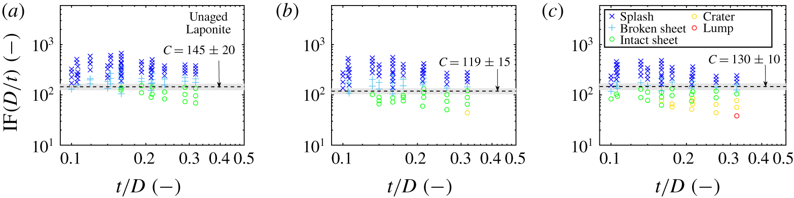
 $\unicode[STIX]{x1D702}_{\infty }$). These rheological properties are the most important in deciding the impact behaviour, provided all other experimental conditions are kept constant. Figure 5 shows the results, plotted using the schemes and conventions mentioned earlier, with the effect of various experimental parameters collapsed into one group, IF
 $(D/t)$.
For all the concentrations of Laponite, we see that the different impact types are effectively separated via this non-dimensionalisation. There is very little overlap between different symbols representing the different impact event types. This is a very encouraging result in itself, and shows that this dimensionless group is able to capture the leading-order physics, and also supports the claim to classify the impact events in the manner that we have done here. We also see that a distinct boundary exists between the ‘splashy’ and ‘sticky’ regimes, which is chosen to be that between broken sheet and intact sheet. This boundary is of almost zero slope, as predicted by (3.3), and gives the value of  $\text{IF}(D/t)=C$ for a transition from stick to splash. Changing any one or a combination of the four parameters may make an event transition from stick to splash, provided the critical value of
 $C$ is crossed during the change. For example, if film thickness
 $t$ is increasing during spray coating, the value of
 $\text{IF}(D/t)$ will decrease and the impact type can change from splash to stick.
Other available dimensionless groups were tested with our data set, as several exist for Newtonian fluid drops impacting wetted surfaces (Cossali et al. Reference Cossali, Coghe and Marengo1997; Josserand & Zaleski Reference Josserand and Zaleski2003; Vander Wal et al. Reference Vander Wal, Berger and Mozes2005a,Reference Vander Wal, Berger and Mozesb). In appendix C, we use one such grouping (C 3) from Cossali et al. (Reference Cossali, Coghe and Marengo1997) to plot regime maps for our results with Laponite, and the results in figure 12 are poor. Regimes are not clearly identified by this other dimensionless grouping.
The success of  $\text{IF}(D/t)=C$ is strengthened by our finding of a similar value of
 $C$ across different concentrations of Laponite,
 $C\approx 130$. The variation is non-monotonic with Laponite concentration and the uncertainty ranges overlap for each formulation. This further substantiates the hypothesis that the rheological properties matter more than just the specific microstructure of the fluid. We test this hypothesis by comparing all Laponite samples to the large data set for Carbopol in Blackwell et al. (Reference Blackwell, Deetjen, Gaudio and Ewoldt2015).
3.4 Comparison of (unaged) Laponite with Carbopol
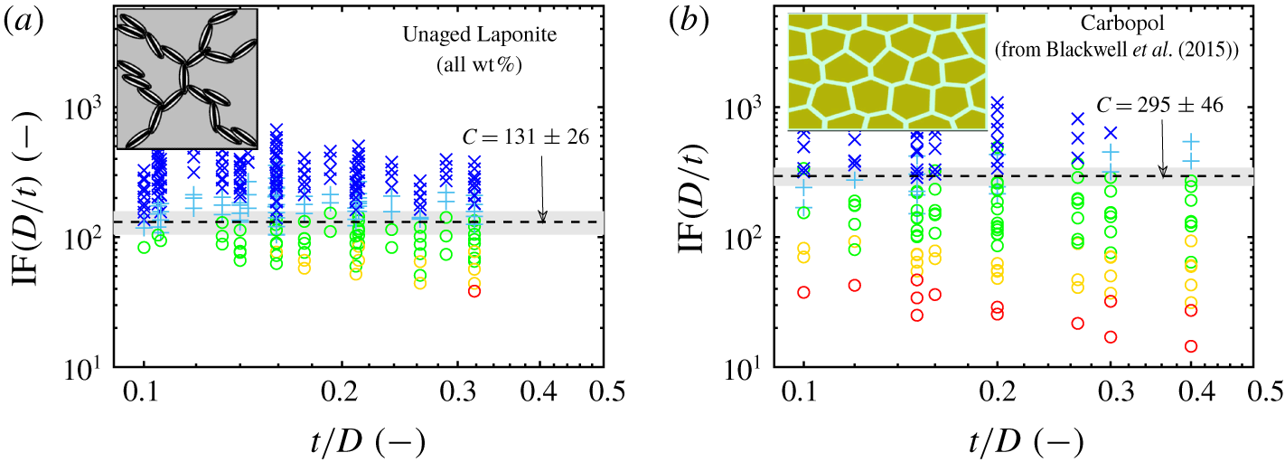
We now test how the value of critical  $C$ may differ for Laponite versus Carbopol. From figure 6(b), it becomes clear that the impact data for Carbopol are also well separated by the scaling into distinct regimes of impact type delineated earlier. The regime map shown is a co-plot of all the concentrations of Carbopol used (0.10, 0.15, 0.25 and 1.00 wt %), but the separation between the regimes is retained (this result was not tested previously in Blackwell et al. (Reference Blackwell, Deetjen, Gaudio and Ewoldt2015)). As a result, one single line of zero slope, a line showing the value of
 $C$, is able to demarcate the boundary between stick and splash types. Thus, the scaling law works well to give an approximate boundary between regimes for a wide range of Carbopol concentrations.
Comparison of regime maps for Carbopol and unaged Laponite. (a) Co-plotting all the results in figure 5 for all three concentrations of Laponite tested. The separation between the regimes is retained and  $C\approx 131$. (b) Reformatted Carbopol impact regime map (Blackwell et al. Reference Blackwell, Deetjen, Gaudio and Ewoldt2015) (the data were plotted in Blackwell et al.’s paper as IF versus
 $t/D$). The concentrations of Carbopol used were 0.10, 0.15, 0.25 and 1.00 wt % (see the supplementary information, section 1, for rheological properties). The co-plots show that the
 $C$ values for the two different fluids are only different by a factor of 2. Carbopol schematic in (b) adapted from Piau (Reference Piau2007), reused with permission.

We see that this critical value of  $C$, which itself is a constant independent of the fluid formulation, is only different by a factor of 2 for Laponite (
 $C\approx 131\pm 26$, figure 6a) and Carbopol (
 $C\approx 295\pm 46$, figure 6b). Thus, not only does the dimensionless group separate the regimes well, the number
 $C$ is a constant independent of the experimental conditions and largely invariant with material chemistry and microstructure. Additional plots of the Bingham number (
 $Bn$) give insight into possible variation in
 $C$ for the two fluids. The Bingham number compares the significance of plasticity (captured by
 $\unicode[STIX]{x1D70E}_{y}$) compared to the viscous rate-dependent stress (
 $K(V/t)^{0.5}+\unicode[STIX]{x1D702}_{\infty }V/t$). A co-plot of IF
 $(D/t)$ versus
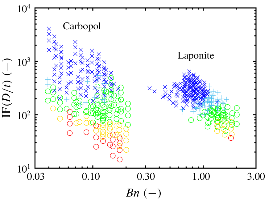
 $Bn$ for Laponite and Carbopol is shown in figure 7, and reflects the flow curves in figure 2.
Co-plots of drop impact data for unaged Laponite and Carbopol, plotted as  $\text{IF}(D/t)$ versus
 $Bn$. For Laponite, the plasticity component is dominant over the viscous stress since
 $Bn\gtrsim 1$ for the stick–splash boundary, whereas for Carbopol it is
 ${<}0.25$, which means the viscous component is dominant.

The primary observation is that the Laponite data lie at higher  $Bn$ (
 $Bn\sim 1$) where the plasticity component is significant. The Laponite conditions are separated completely from the Carbopol conditions, for which the viscous component dominates and
 $Bn<0.25$. This difference is rationalised from the flow curves, where Carbopol stresses increase more rapidly with strain rate. Secondly, we observe a possible
 $Bn$-dependence on the regime boundaries for Laponite around
 $Bn=1$, apparent between the two splashy types of impact (splash and broken sheet) and possibly also between broken and intact sheets. The apparent increase in
 $C$ with
 $Bn$ for Laponite cannot rationalise the difference in
 $C$ between Laponite and Carbopol, since the opposite trend is needed to connect the regime boundaries at the same value of
 $C$ in the same range of
 $Bn$. Yet, there is additional insight from the
 $Bn$ dependence near
 $Bn=1$, in that one needs greater IF
 $(D/t)$ values to produce a splash as the significance of the plastic component dominates. This suggests additional resistive/dissipative forces acting in Laponite at lower shear rates (
 $Bn>1$) that are not captured in the steady flow description. A possible reason could be the use of a ‘dynamic’ instead of a ‘static’
 $\unicode[STIX]{x1D70E}_{y}$ in describing the rheology of Laponite, and using it to define IF. As we increase
 $Bn$, the yield stress becomes more significant, and the (higher) static yield stress to initiate flow may be more important than the (lower) dynamic yield stress to arrest the flow. Partial thixotropic aging and/or incomplete breakdown of structures upon impact can also introduce additional dissipative forces that are initially larger and decay down to the steady behaviour used to calculate IF. We note that viscoelasticity would give the opposite trend, since stresses transiently grow upon start up of flow, in contrast to thixotropic stress decay to steady state.
Other arguments to rationalise this difference in  $C$ can include extensibility of fluids tested. Carbopol is possibly more extensible than Laponite (Nelson & Ewoldt Reference Nelson and Ewoldt2017), and so using only shear properties is not sufficient when drop impacts involve large strain rates, both in shear and extension. Microstructurally, Carbopol is a polymeric system, and Laponite is more brittle, so we might expect some extensional thickening behaviour in the polymer-based systems. Even if Carbopol is thinning in extension (Louvet, Bonn & Kellay Reference Louvet, Bonn and Kellay2014), one may expect higher critical values of
 $C$ if there is a higher ratio of extensional to shear viscosity (Trouton ratio) compared to Laponite. This makes its drop impact behaviour different from Laponite. We intend to address the role of extensional properties in future work by controlling variable extensional rheology of Carbopol while maintaining the shear properties, similar to the variable extensional properties of yield stress fluid formulations for direct-write 3D printing described in Rauzan et al. (Reference Rauzan, Nelson, Lehman, Ewoldt and Nuzzo2018). This should allow us to access the effect of extensional thickening due to the large extension rates during drop impacts, and may help explain why polymeric systems such as Carbopol may require larger inertial stresses to splash compared to clay-based systems such as Laponite. Such a study is also work in progress.
It must be noted that the calculated value of the dimensionless group IF is sensitive to the rheological fit parameters, and therefore sensitive to the available steady flow data. The range of shear rates, density of data points, uncertainties in measured data and the quality of fit of the rheological model all contribute to the rheological parameter values and uncertainties, which are used in the calculation of IF. The sensitivity of IF propagates to the sensitivity of the critical value  $C$ to changes in the available parent data. As shown in the supplementary information, § 6, we observed an increase in IF and
 $C$ when the range of applied shear rates for the flow curves was expanded from
 $0.1{-}100~\text{s}^{-1}$ to
 $0.01{-}1000~\text{s}^{-1}$ (the flow curve using the narrower range is shown in the supplementary information, § 6.1, figure S8). The regime maps using this narrower range of rheology data are shown for both fluids (figure S9), and we see that the values of
 $C$ were
 $74\pm 3$ and
 $75\pm 8$ for Laponite and Carbopol respectively, compared to
 $118\pm 24$ and
 $205\pm 50$ using the expanded, currently used data set, shown in figure S10. Here we have used the Bingham model to fit the rheological data, following the original definition of IF in Blackwell et al. (Reference Blackwell, Deetjen, Gaudio and Ewoldt2015). The choice of rheological model used for the fit also plays a role in the calculation of IF. Regime maps in § 6.2 in the supplementary information show this dependence of fitting different models to the same data set (with the wider range of shear rates). Since all models are reductions of the actual, complete data, the underlying physics can never be captured fully. There always lies some variability between different model fits, and dimensionless groups inherit this variability.
In spite of these caveats,  $C$ is comparable to the same order of magnitude for two vastly different yield-stress systems: Laponite clay, an appreciably thixotropic suspension, formed of charged, rigid discs coming together in a stacked structure to form a soft gel, and Carbopol, a jammed gel consisting of soft polymer microgel particles with negligible thixotropy. This in itself is a milestone observation.
We have chosen the boundary between broken sheet–intact sheet as the transition between stick and splash, which dictates the value of critical  $C$ we obtain. The boundary of interest can also be chosen as that between splash–broken sheet, intact sheet–crater, etc. These lead to different values of
 $C$, and this alternative method has been illustrated further with different values of
 $C$ obtained in the supplementary information (figure S4 and table S3). But no matter what boundary is chosen to find
 $C$, we see that (i) the separation between the regimes is retained (which does not depend on the choice of the boundary anyway), (ii) the value of
 $C$ remains nearly constant for all formulations of a given fluid and (iii) the values for Laponite and Carbopol only differ by a factor of 2, so are essentially of the same order of magnitude within experimental errors. This supports a general conclusion of the paper: the macroscopic behaviour is mostly the same, regardless of the microstructure, although the critical value of
 $C$ varies by about a factor of 2 for the two fluids. The difference could be even larger in other cases. We use only steady shear rheological properties to estimate the dissipative flow stresses, which are comparable between the two fluids used. However, rheological properties are multi-dimensional, and it is not possible to match each and every property for two microstructurally distinct fluids. It is a philosophical question for high-dimensional rheology data: for two different microstructures, can all of the rheological properties truly be the same? Or the more useful question: can the important rheological properties be the same? This is what is required for the microstructure agnostic, abstracted physical concepts to be valid. The applicability of these results are in spray coating and painting, fire suppression, etc., where the main concern is to suppress/promote ‘splashy’ behaviour as and when needed. Thus, we anticipate that the most relevant boundary to look at is between intact sheet and broken sheet since this represents the characteristic behaviour of a material to stick or splash, the same reason why this is the specific boundary studied in this work.
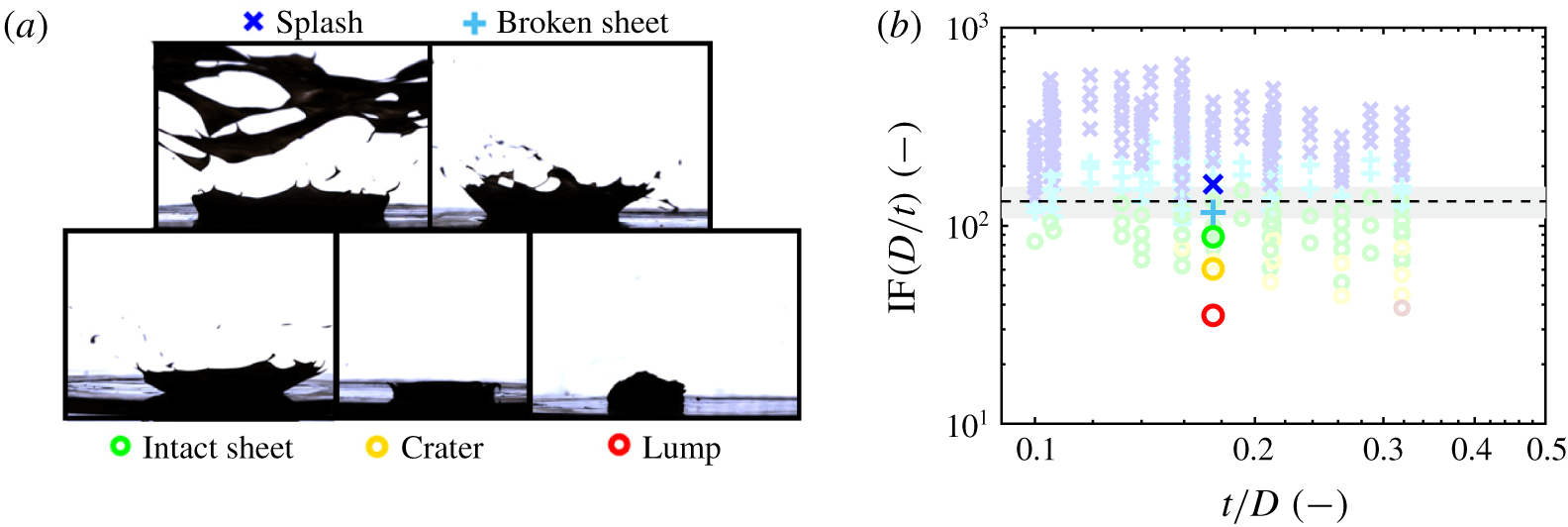
Drop impact results for Bentonite. (a) Various impact events observed during experiments. (b) One-off drop impact tests with Bentonite plotted using  $\text{IF}(D/t)$, co-plotted with results for Laponite.

4 Summary and discussion
We have tested a dimensionless group for drop impact with non-Newtonian yield-stress fluids having different chemistry and microstructure. This critical value IF $(D/t)\approx C$ is observed to be constant over a range of different experimental parameters, the value of the constant does not change with material formulation (concentration), and the values are different by a factor of 2 for two microstructurally distinct yield-stress fluids (Laponite and Carbopol) covering the two key routes to achieve a yield-stress fluid (Nelson & Ewoldt Reference Nelson and Ewoldt2017). These have different chemical structure and morphology: an attractive gel network from rigid discs of Laponite versus a crowded jammed suspension from soft microgel particles of Carbopol. Yet, the steady-state flow properties are sufficient for the regime maps, and a common condition can be obtained for predicting stick/splash behaviour. The boundary is chosen to be that between broken sheet and intact sheet since it is the most relevant transition between stick–splash regimes in applications deemed to benefit from this work (spray coating, fire suppression, etc.).
To further assess the robustness of this dimensionless group, we tested a few conditions of drop impact with another common clay, Bentonite, at 13 wt % in water which forms a yield-stress fluid. By changing the velocity of impact, all five different types of splash were observed. The critical values of transition are similar to the Laponite data (figure 8), although the stick–splash transition value of  $C$ is slightly lower for this sample of Bentonite. The reason could be that the flow curve of Bentonite looks similar to that for Laponite. The general behaviour of the shear stress with imposed rates (dictated by
 $V$ and
 $t$) would thus be similar. This also makes physical sense since both are clays. The drop impact behaviour for Bentonite is consequently similar, although more tests need to be done to ascertain the regime boundary more accurately. Nevertheless, these tests provide additional evidence for the validity of this group, and further studies with different yield-stress fluids will provide valuable assessment of the robustness of this scaling. Full details, including flow curves for Bentonite and experimental details have been shown in the supplementary information, § 7.
We have assumed other effects including surface tension, and thixotropy, apart from extensional rheology properties, to be insignificant. These assumptions simplify the study drastically. So it would be of no surprise if the scaling law fails if we test fluids with significant extensibility, as seen with Carbopol (which can be significant and even desirable for certain yield-stress fluids (Nelson et al. Reference Nelson, Bras, Liu and Ewoldt2018; Rauzan et al. Reference Rauzan, Nelson, Lehman, Ewoldt and Nuzzo2018)), allow thixotropic aging to occur, which can change material microstructure and macroscopic properties or probe scenarios where surface tension effects become comparable with viscous and inertial stresses, e.g. at much smaller droplet sizes which are difficult to produce in our set-up (and may need to be studied as spray rather than isolated individual droplets). It is still a very curious result that neglecting surface tension should collapse data this well. This may be because surface tension values do not vary across the different samples, but also because many of the impact types do not generate sheet breakup. Surface tension does play a major role in sheet breakup, but the different types of splash may emphasise dynamics related to initial moments of the impact, rather than the later stages (e.g. we do not consider drop size distribution in our work here). For sheets that are smaller or non-existent (cases of intact sheet, crater and lump), surface tension is not dominant over the yield stress since sheet breakup never occurs.
We have neglected the influence of elasticity in our tests. Historically, yield-stress fluids have been modelled as elastic solids before yielding; post-yield, usually modelled as highly viscous fluids (Dinkgreve et al. Reference Dinkgreve, Paredes, Denn and Bonn2016). In figure 2, the elastic data shown are for very small oscillatory strain amplitudes, and this is in the unyielded regime where the material is predominantly solid like. The dimensionless group IF neglects elasticity (linear elasticity before yield, and normal stresses after yield), as if the fluid yields and behaves as a viscoplastic fluid. This assumption can fail for materials that have appreciable extensional thickening, where viscoelastic transients due to the presence of polymeric components can alter the impact behaviour. Since Carbopol is a polymeric microgel colloid, it may have more elasticity in extension, and this may be the cause for the higher critical value (e.g. higher velocity needed) for splash. Even a variable power-law index for the fluids tested, dependent on the applied rate, can affect the results (Louvet et al. Reference Louvet, Bonn and Kellay2014).
Extreme values of the normalised coating thickness ( $t/D$) may also make the situation more complicated, necessitating the use of additional dimensionless groups instead of the single one of (1.2c). Dissipation decreases with smaller film thickness. We note that dissipation could also decrease due to a slip condition between the liquid and the solid, e.g. as reported by Luu & Forterre (Reference Luu and Forterre2013) with yield-stress fluid (Carbopol) impacts onto dry hydrophobic surfaces.
With these possible limitations in mind, the group tested here has already proven useful in predicting splash behaviour for diverse fluids with complex formulation and microstructure, such as paints. For example, we can rationalise the conditions required for artists to employ a technique where small droplets (0.1–5 mm) impinge on the edge of a small pool of paint to form a splash crown with colour on two sides and edges that roll up to eventually form paint spirals (Truscott et al. Reference Truscott, Darbois-Texier, Lovett, Brandenbourger, Maquet, Pan, Gilet, Strivay and Dorbola2015). The paint rheology was measured and fit to the Bingham model and the value of IF $(D/t)$ used by artists, who must release the drop from sufficient height
 $h$, was found to be above the predicted ‘splash’ regime (T. Truscott, personal communication, 2015).
Yield-stress fluids also find creative use in spraying for suppressing, controlling and mitigating forest fires (Yu et al. Reference Yu, Chen, Chan, Agmon, Stapleton, Sevit, Tibbitt, Acosta, Zhang and Franzia2016; Blackwell Reference Blackwell2017). Retardants can be mixed with a suitably designed fluid with targeted range of  $C$ under typical spraying conditions employed by firefighters. These fluids can coat the substrates (e.g. forest vegetation), stay intact upon cessation of flow and also prevent further erosion by wind or rain, an aspect which can be incorporated into the fluid design. Similarly relevant applications involve spray painting and spray coating. In all of these cases, caution should be used to be aware of other rheological properties that may become important in different limits, such as thixotropic, viscoelastic and extensional rheology effects.
Acknowledgements
This work was funded by the National Science Foundation, CAREER Award, CBET-1351342. S.S. acknowledges the PPG Foundation for partial support through a PPG-MRL Graduate Research Assistantship at the University of Illinois at Urbana-Champaign. We thank Dr G. Chaudhary for helpful feedback and discussions.
Declaration of interests
The authors report no conflict of interest.
Supplementary movies and materials
Supplementary movies and materials are available at https://doi.org/10.1017/jfm.2020.147.
Appendix A. Effect of each experimental parameter on drop impact
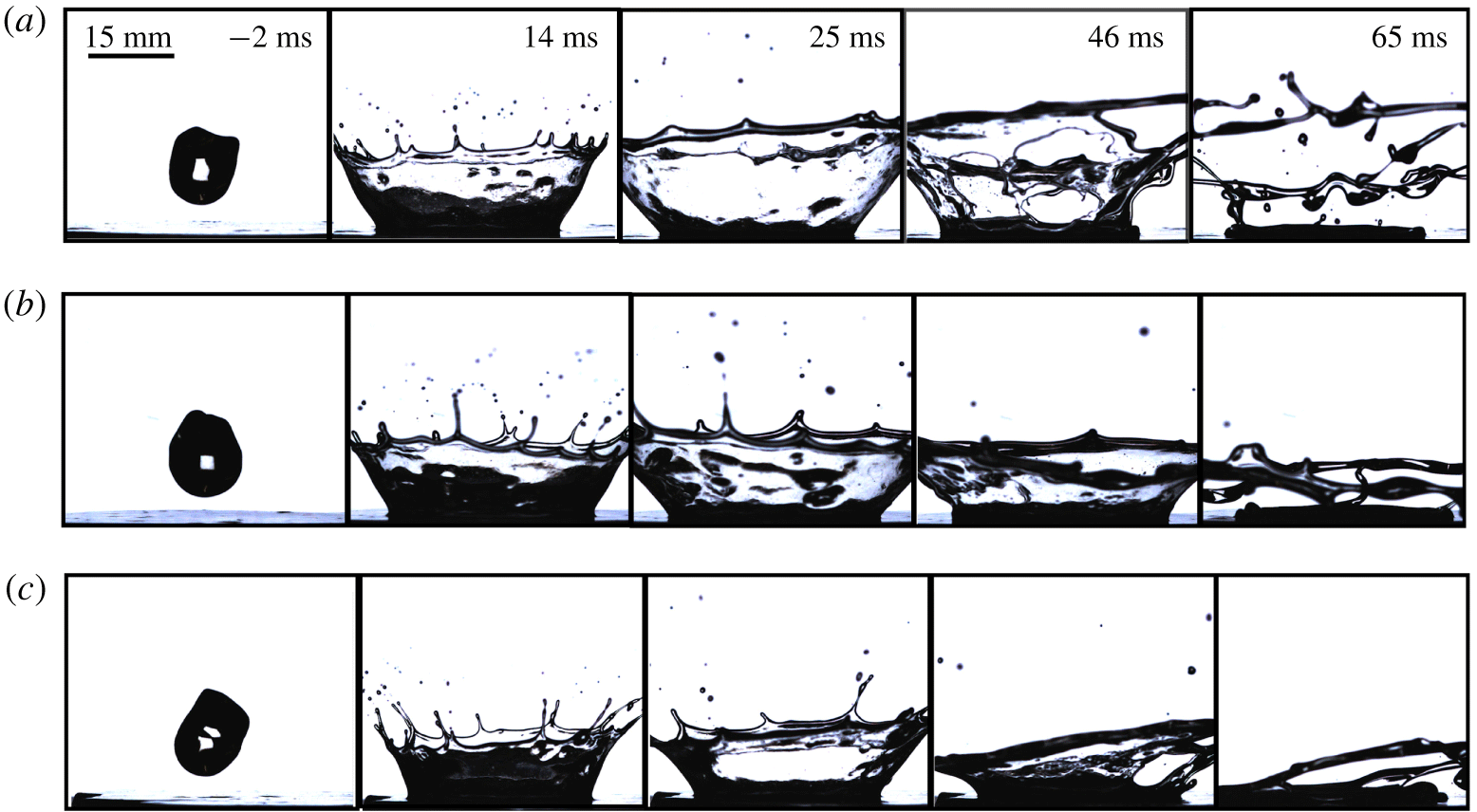
Figures 9–11 show additional representative examples for the effect of varying each experimental parameter on drop impact outcome. These complement figure 3 which showed the effect of varying the impact velocity.
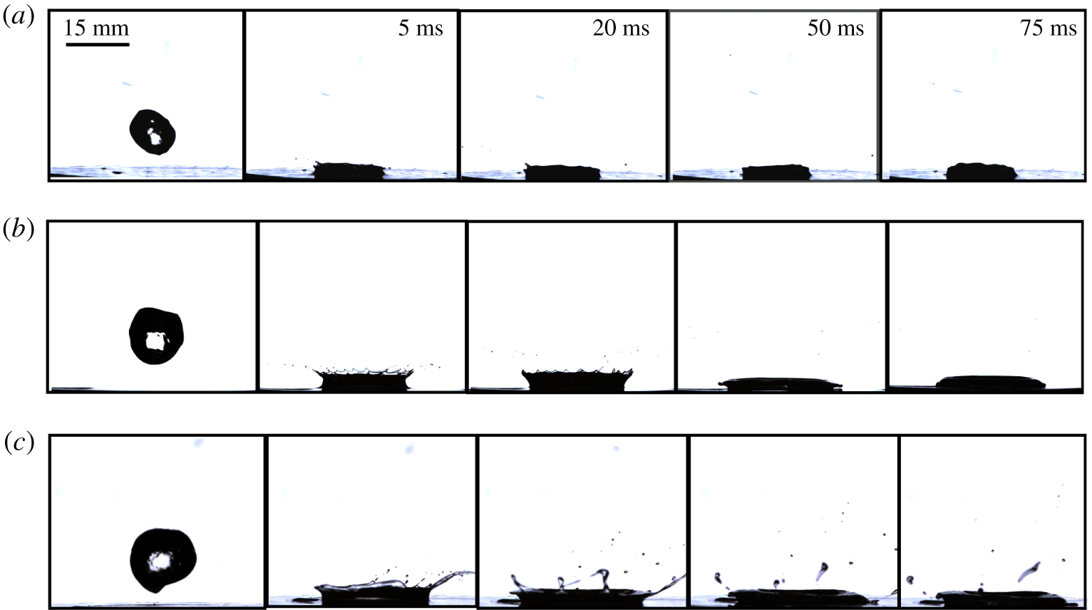
In figure 9, we see the effect of increasing the concentration of Laponite. The impact type is a broken sheet for each of 3.5 and 4.0 wt %, while it is an intact sheet for 4.5 wt %. Larger concentrations have larger values of  $\unicode[STIX]{x1D70E}_{y}$,
 $K$, and
 $\unicode[STIX]{x1D702}_{\infty }$, and thus dissipative forces dominate over inertial forces to make the impact type more ‘stick’ as particle loading increases.
Figure 10 shows the effect of varying the drop diameter. Larger drops have greater inertial forces for the same dissipative forces, and hence ‘splash’ more. The impact type is a lump for the 10 mm drop, while a crater is formed upon impact for both 15 and 20 mm drops.
Lastly, figure 11 shows the effect of coating thickness. It might seem at first that lower thicknesses would lead to higher shear rates, and dissipative stresses would dominate. But since the group compares forces rather than stresses, and the dissipative forces decrease as the coating gets thinner, more ‘splash’ occurs at lower coating thicknesses.
Effect of varying concentration. Drops of  $D=10~\text{mm}$, impacting a
 $t=2.9~\text{mm}$ thick coating at
 $V=4~\text{m}~\text{s}^{-1}$, with the Laponite concentration being (a)
 $c=3.5$, (b)
 $4.0$ and (c) 4.5 wt %. For the same experimental conditions, samples splash less as the concentration increases, since dissipative forces are larger at higher loadings.

Effect of varying drop size. Drops of 4.0 wt % Laponite impacting a  $t=3.2~\text{mm}$ thick coating of the same material at
 $2~\text{m}~\text{s}^{-1}$, with drop diameters being (a)
 $D=10$, (b)
 $15$ and (c) 20 mm. For the same experimental conditions, samples splash more as the drop diameter is increased, which is expected, since the inertial forces, which are responsible for promoting splash, increase with size.

Effect of varying coating thickness. Drops of  $D=15~\text{mm}$, 3.5 wt % Laponite at
 $V=3~\text{m}~\text{s}^{-1}$ impacting coatings with thicknesses (a)
 $t=1.5$, (b)
 $2.1$ and (c) 2.9 mm. For the same experimental conditions, samples splash less as the coating thickness is increased, which is expected, since dissipative forces are greater.

Appendix B. Obtaining  $C$ from regime maps

We fit the equation of a line to the set of points that form the boundary between a broken sheet behaviour in the regime maps ( $p^{BS}$) and an intact sheet behaviour (
 $p^{IS}$). The points to be considered for: (i) broken sheet are those that have the lowest values of IF
 $(D/t)$ (set of
 $p^{BS}$), and for (ii) intact sheet are those that have the highest values of IF
 $(D/t)$ (set of
 $p^{IS}$). In this way, we are fitting a line to the points that demarcate the lower and upper boundaries of broken and intact sheet regimes, respectively. Note that, as mentioned earlier, we limit the values of
 $t/D$ to be greater than 0.1. We treat the values of IF
 $\left(D/t\right)$ as
 $y$ data, the corresponding values of
 $t/D$ as
 $x$ data and fit a function to this data set of
 $y$ versus
 $x$, wherein the function is that of a line in slope-intercept form. The equation to be fit is
 $$\begin{eqnarray}y(\{p^{BS},p^{IS}\})=mx+C.\end{eqnarray}$$
In the process, we obtain the slope,  $m$, and intercept,
 $C$, of this line. We can force
 $m$ to be exactly 0, so that we obtain the value of
 $C$ for which the regime boundary is a constant. The uncertainty values reported are the 95 % confidence bounds on the parameter probabilities obtained from the fit, which uses a library function in MATLAB (lsqcurvefit) to find the optimal value of
 $C$ for the minimum residual. The confidence bounds are obtained from the fit using the library routine
nlparci.
Appendix C. Regime maps with other dimensionless numbers
To further strengthen the validity of the hypothesised dimensionless group, here we show the drop impact results on maps using two different dimensionless groups. These groups are generally used for Newtonian fluids with very good results, obtaining critical values for a splash upon impact, as well as a proper separation of impact regimes.
In figure 12(a), the regime map for drop impact results for Laponite is plotted using a dimensionless group used for Newtonian fluid droplets impacting a wetted solid surface (Cossali et al. Reference Cossali, Coghe and Marengo1997). This correlation is based on two dimensionless groups, the Weber number,
 $$\begin{eqnarray}We\equiv \frac{\unicode[STIX]{x1D70C}V^{2}D}{\unicode[STIX]{x1D6FE}},\end{eqnarray}$$
and the Ohnesorge number,
 $$\begin{eqnarray}Oh\equiv \frac{\unicode[STIX]{x1D702}}{\sqrt{\unicode[STIX]{x1D70C}\unicode[STIX]{x1D6FE}D}},\end{eqnarray}$$
where  $\unicode[STIX]{x1D70C}$,
 $\unicode[STIX]{x1D6FE}$,
 $\unicode[STIX]{x1D702}$ and
 $D$ are the density, surface tension, viscosity and diameter of the fluid drop respectively. The correlation based on these is defined as
 $$\begin{eqnarray}Y=\frac{We\,Oh^{-0.4}}{2100+5880(t/D)^{1.44}},\end{eqnarray}$$
and a splash is predicted for  $Y\geqslant 1$.
For our data, we use  $\unicode[STIX]{x1D702}_{\infty }$ in place of
 $\unicode[STIX]{x1D702}$. It is clear from figure 12(a) that this non-dimensionalisation is unsuccessful for use with Laponite. The separation between the regimes is not maintained. Although there is a general trend of increased ‘splash’ as we go to higher values of the ordinate, no single critical value for a transition from stick-to-splash can be deduced.
Performance of two other dimensionless groups with drop impact data for Laponite. (a) Dimensionless group outlined in (C 3) plotted versus  $t/D$. The separation between different regimes is not retained; moreover, there is no clear constant value that shows the onset of stick–splash transition. (b) Reynolds number based on
 $\unicode[STIX]{x1D702}_{\infty }$ obtained from fits to the Bingham model. Unlike IF
 $(D/t)$, the absence of
 $\unicode[STIX]{x1D70E}_{y}$ in the group impairs its predictive capability. There is a lot of overlap between impact regimes, and consequently no constant critical value of Re for the stick–splash transition.

Figure 12(b) shows a regime map plotted using a Reynolds number ( $Re$) based on
 $\unicode[STIX]{x1D702}_{\infty }$. As mentioned earlier, omitting the
 $\unicode[STIX]{x1D70E}_{y}$ from IF simplifies to this form of
 $Re$, and it does not work well to separate the regimes. Consequently, no single critical value of
 $Re$ can be obtained for the ‘splash’ transition, although the general trend again is physically intuitive; higher
 $Re$ implies an increase of drop and sheet breakup.