2.1 Equations of motion

The mathematical model and its stability analysis in the present study are based on those described in Hwang & Pedley (Reference Hwang and Pedley2014a ). This model is derived from the Navier–Stokes equations combined with a Smoluchowski equation describing the cell distribution in time, space and cell-orientation space. The model adopts the translational diffusivity expression proposed by Pedley & Kessler (Reference Pedley and Kessler1990), although this can be improved by the generalised Taylor’s dispersion theory (for example, Hill & Bees Reference Hill and Bees2002). In our presentation here, we have omitted repeated details for brevity. Suppose we have a fluid of density, $\unicode[STIX]{x1D70C}$ , and kinematic viscosity, $\unicode[STIX]{x1D708}$ , in an infinitely long and infinitely wide channel, subject to a constant pressure gradient in the horizontal direction. Here, we denote $x^{\ast }$ , $y^{\ast }$ and $z^{\ast }$ as the streamwise, vertical and spanwise directions, respectively, and $t^{\ast }$ as the time (note that the superscript $^{\ast }$ denotes dimensional variables). The two walls of the channel are located at $y^{\ast }=\pm h$ , where $h$ is half-height of the channel. In this horizontal channel there is a suspension of spherical gyrotactic cells with average cell-number density, $N$ . The individual cell is assumed to swim at speed $V_{c}^{\ast }$ and is subject to gravity, as well as diffusion. The cell sedimentation speed is given by $V_{s}^{\ast }$ , and, as we shall see in § 3.1, plays a crucial role in the formation of the gyrotactically trapped equilibrium layer. The swimming direction of the cells is denoted by a unit vector, $\boldsymbol{e}=(e_{1},e_{2},e_{3})$ , and their sedimentation direction is $-\boldsymbol{j}$ (where $\boldsymbol{j}$ is the upward unit vector in the vertical direction). As shown in Pedley & Kessler (Reference Pedley and Kessler1990), the translational diffusivity of the suspension scales like ${V_{c}^{\ast }}^{2}\unicode[STIX]{x1D70F}$ , where $\unicode[STIX]{x1D70F}$ is the swimming direction correlation time. We use this as the representative value for translational diffusivity, such that $D_{V}\equiv {V_{c}^{\ast }}^{2}\unicode[STIX]{x1D70F}$ . Using the length scale $h$ , the diffusion velocity scale $D_{V}/h$ , and the average cell-number density $N$ , the dimensionless equations of motion are:

(2.1a ) $$\begin{eqnarray}\displaystyle & \displaystyle \unicode[STIX]{x1D735}\boldsymbol{\cdot }\boldsymbol{u}=0, & \displaystyle\end{eqnarray}$$

(2.1b ) $$\begin{eqnarray}\displaystyle & \displaystyle \mathit{Sc}^{-1}\left(\displaystyle \frac{\unicode[STIX]{x2202}\boldsymbol{u}}{\unicode[STIX]{x2202}t}+(\boldsymbol{u}\boldsymbol{\cdot }\unicode[STIX]{x1D735})\boldsymbol{u}\right)=-\unicode[STIX]{x1D735}p+\unicode[STIX]{x1D6FB}^{2}\boldsymbol{u}-\mathit{Ra}~n\boldsymbol{j}, & \displaystyle\end{eqnarray}$$

(2.1c ) $$\begin{eqnarray}\displaystyle & \displaystyle \displaystyle \frac{\unicode[STIX]{x2202}n}{\unicode[STIX]{x2202}t}+\unicode[STIX]{x1D735}\boldsymbol{\cdot }[n(\boldsymbol{u}+V_{c}\langle \boldsymbol{e}\rangle -V_{s}\,\boldsymbol{j})]=\unicode[STIX]{x1D735}\boldsymbol{\cdot }(\unicode[STIX]{x1D63F}_{T}\boldsymbol{\cdot }\unicode[STIX]{x1D735}n), & \displaystyle\end{eqnarray}$$

with the no-slip and no-flux boundary conditions on the walls

(2.1d ) $$\begin{eqnarray}\displaystyle & \displaystyle \boldsymbol{u}|_{y=\pm 1}=(0,0,0), & \displaystyle\end{eqnarray}$$

(2.1e ) $$\begin{eqnarray}\displaystyle & \displaystyle [n(\boldsymbol{u}+V_{c}\langle \boldsymbol{e}\rangle -V_{s}\,\boldsymbol{j})-\unicode[STIX]{x1D63F}_{T}\boldsymbol{\cdot }\unicode[STIX]{x1D735}n]|_{y=\pm 1}\boldsymbol{\cdot }\boldsymbol{j}=0, & \displaystyle\end{eqnarray}$$

where $\boldsymbol{u}(=(u,v,w))$ , $p$ , $n$ , $V_{c}$ , $V_{s}$ and $\unicode[STIX]{x1D63F}_{T}$ ( $\equiv \langle A\boldsymbol{A}\rangle -\langle \boldsymbol{e}\rangle \langle \boldsymbol{e}\rangle$ ; see also Pedley & Kessler (Reference Pedley and Kessler1990) for this expression), are the dimensionless velocity, pressure, cell-number density, cell-swimming speed, cell sedimentation speed, and translational diffusivity tensor, respectively. The Schmidt number $Sc$ and the Rayleigh number $Ra$ in (2.1b ) are given by

(2.1f,g ) $$\begin{eqnarray}\mathit{Sc}={\displaystyle \frac{\unicode[STIX]{x1D708}}{D_{V}}}\quad \text{and}\quad \mathit{Ra}={\displaystyle \frac{N\unicode[STIX]{x1D710}g^{\prime }h^{3}}{D_{V}\unicode[STIX]{x1D708}}},\end{eqnarray}$$

where $g^{\prime }=g\unicode[STIX]{x0394}\unicode[STIX]{x1D70C}/\unicode[STIX]{x1D70C}$ is the reduced gravity ( $\unicode[STIX]{x0394}\unicode[STIX]{x1D70C}$ is the density difference between the cell and fluid) and $\unicode[STIX]{x1D710}$ the volume of a cell. In (2.1c ) and (2.1e ), $\langle \cdot \rangle$ denotes the local ensemble average at given spatial location $\boldsymbol{x}$ , which is obtained with the p.d.f. of the cell-swimming orientation, $f(\boldsymbol{x},\boldsymbol{e},t)$ . This satisfies

(2.1h ) $$\begin{eqnarray}D_{R}^{-1}\displaystyle \frac{\unicode[STIX]{x2202}f}{\unicode[STIX]{x2202}t}+D_{R}^{-1}(\boldsymbol{u}\boldsymbol{\cdot }\unicode[STIX]{x1D735})f+\unicode[STIX]{x1D735}_{e}\boldsymbol{\cdot }\left(\unicode[STIX]{x1D706}(\boldsymbol{j}-(\boldsymbol{j}\boldsymbol{\cdot }\boldsymbol{e})\boldsymbol{e})f+{\displaystyle \frac{\unicode[STIX]{x1D734}}{2D_{R}}}\times \boldsymbol{e}f\right)=\unicode[STIX]{x1D6FB}_{e}^{2}f,\end{eqnarray}$$

where $\unicode[STIX]{x1D734}$ is the flow vorticity. Here, the dimensionless rotational diffusivity $D_{R}$ and the dimensionless inverse of the gyrotactic time scale $\unicode[STIX]{x1D706}$ are also given by

(2.1i,j ) $$\begin{eqnarray}D_{R}\equiv \frac{D_{R}^{\ast }h^{2}}{D_{V}}\quad \text{and}\quad \unicode[STIX]{x1D706}=\frac{1}{2BD_{R}^{\ast }},\end{eqnarray}$$

with the rotational diffusivity $D_{R}^{\ast }$ and the gyrotactic time scale $B$ .

2.2 Basic state

Given the horizontal homogeneity of the flow, equation (2.1) admits the following equilibrium solution:

(2.2a ) $$\begin{eqnarray}\boldsymbol{u}_{0}(y)=(U_{0}(y),0,0),\quad n=n_{0}(y),\end{eqnarray}$$

where

(2.2b ) $$\begin{eqnarray}\displaystyle & \displaystyle U_{0}(y)=\mathit{Sc}Re(1-y^{2}), & \displaystyle\end{eqnarray}$$

(2.2c ) $$\begin{eqnarray}\displaystyle & \displaystyle n_{0}(y)=N_{0}\exp \left(\int {\displaystyle \frac{V_{c}\langle e_{2}\rangle _{0}-V_{s}}{D_{T0}^{22}}}\text{d}y\right). & \displaystyle\end{eqnarray}$$

Here, $Re=U_{c}h/\unicode[STIX]{x1D708}$ is the Reynolds number based on the centreline velocity $U_{c}$ , and $N_{0}$ is the normalisation constant setting the volume average of $n_{0}(y)$ to be unity. Also, in (2.2c ), $\langle \boldsymbol{\cdot }\rangle _{0}$ is obtained from the steady and horizontally uniform solution $f_{0}$ of (2.1h ): i.e.

(2.2d ) $$\begin{eqnarray}\unicode[STIX]{x1D735}_{e}\boldsymbol{\cdot }\left(\unicode[STIX]{x1D706}(\boldsymbol{j}-(\boldsymbol{j}\boldsymbol{\cdot }\boldsymbol{e})\boldsymbol{e})f_{0}+{\displaystyle \frac{\unicode[STIX]{x1D734}_{0}}{2D_{R}}}\times \boldsymbol{e}f_{0}\right)=\unicode[STIX]{x1D6FB}_{e}^{2}f_{0},\end{eqnarray}$$

where $\unicode[STIX]{x1D734}_{0}=(0,0,-ScRe(\text{d}U_{0}/\text{d}y))$ .

In the regime of high shear rates, one may estimate the formation time scale of the basic state from an initially uniform suspension. In this case, the effect of the upswimming velocity would be negligible due to very high surrounding shear. Therefore, the time scale for layer formation will be given by the length scale of the system and translational diffusivity, such that

(2.3) $$\begin{eqnarray}T_{layer}\sim \frac{h^{2}}{D_{V}^{\ast }}=\frac{(0.25)^{2}}{1.98\times 10^{-4}}\approx 300~\text{s}.\end{eqnarray}$$

2.3 Linear stability analysis

Now, let us consider a small perturbation around the basic state, such that: $[\boldsymbol{u}~n~f]^{\text{T}}=[\boldsymbol{u}_{0}~n_{0}~f_{0}]^{\text{T}}+\unicode[STIX]{x1D716}[\boldsymbol{u}^{\prime }~n^{\prime }~f^{\prime }]^{\text{T}}+O(\unicode[STIX]{x1D716}^{2})$ for $\unicode[STIX]{x1D716}\ll 1$ . The normal-mode solution of the perturbation is then written as

(2.4) $$\begin{eqnarray}[\boldsymbol{u}^{\prime }~n^{\prime }~f^{\prime }]^{\text{T}}(x,y,z,t)=[\hat{\boldsymbol{u}}~\hat{n}~\hat{f}]^{\text{T}}\text{e}^{\text{i}(\unicode[STIX]{x1D6FC}x+\unicode[STIX]{x1D6FD}z-\unicode[STIX]{x1D714}t)}+\text{c.c},\end{eqnarray}$$

where $\unicode[STIX]{x1D714}$ is the unknown complex angular frequency, and $\unicode[STIX]{x1D6FC}$ and $\unicode[STIX]{x1D6FD}$ are the given streamwise and spanwise wavenumbers, respectively. Using the standard procedure that eliminates pressure perturbation, the vertical velocity and vorticity form of the linearised equations of motion are given by

(2.5a ) $$\begin{eqnarray}\text{i}\unicode[STIX]{x1D714}\left(\begin{array}{@{}ccc@{}}\mathit{Sc}^{-1}(k^{2}-{\mathcal{D}}^{2}) & 0 & 0\\ 0 & \mathit{Sc}^{-1} & 0\\ 0 & 0 & 1\end{array}\right)\left(\begin{array}{@{}c@{}}\hat{v}\\ \hat{\unicode[STIX]{x1D702}}\\ \hat{n}\end{array}\right)=\left(\begin{array}{@{}ccc@{}}L_{OS} & 0 & k^{2}\mathit{Ra}\\ \text{i}\unicode[STIX]{x1D6FD}Re{\mathcal{D}}U & L_{SQ} & 0\\ {\mathcal{D}}n_{0}+L_{C}^{v} & L_{C}^{\unicode[STIX]{x1D702}} & L_{C}\end{array}\right)\left(\begin{array}{@{}c@{}}\hat{v}\\ \hat{\unicode[STIX]{x1D702}}\\ \hat{n}\end{array}\right),\end{eqnarray}$$

where

(2.5b ) $$\begin{eqnarray}\displaystyle L_{OS} & = & \displaystyle \text{i}\unicode[STIX]{x1D6FC}ReU(k^{2}-{\mathcal{D}}^{2})+\text{i}\unicode[STIX]{x1D6FC}Re{\mathcal{D}}^{2}U+(k^{2}-{\mathcal{D}}^{2})^{2},\end{eqnarray}$$

(2.5c ) $$\begin{eqnarray}\displaystyle L_{SQ} & = & \displaystyle \text{i}\unicode[STIX]{x1D6FC}ReU+(k^{2}-{\mathcal{D}}^{2}),\end{eqnarray}$$

(2.5d ) $$\begin{eqnarray}\displaystyle L_{C} & = & \displaystyle \text{i}\unicode[STIX]{x1D6FC}\mathit{Sc}ReU+\text{i}\unicode[STIX]{x1D6FC}V_{c}\langle e_{1}\rangle _{0}+(V_{c}\langle e_{2}\rangle _{0}-V_{s}){\mathcal{D}}+\text{i}\unicode[STIX]{x1D6FD}V_{c}\langle e_{3}\rangle _{0}+V_{c}{\mathcal{D}}\langle e_{2}\rangle _{0}\nonumber\\ \displaystyle & & \displaystyle +\,\unicode[STIX]{x1D6FC}^{2}D_{T0}^{11}-2\text{i}\unicode[STIX]{x1D6FC}D_{T0}^{12}{\mathcal{D}}-D_{T0}^{22}{\mathcal{D}}^{2}+\unicode[STIX]{x1D6FD}^{2}D_{T0}^{33}-\text{i}\unicode[STIX]{x1D6FC}{\mathcal{D}}D_{T0}^{12}-{\mathcal{D}}D_{T0}^{22}{\mathcal{D}},\end{eqnarray}$$

(2.5e ) $$\begin{eqnarray}\displaystyle L_{C}^{v} & = & \displaystyle \left[G_{1}{\mathcal{D}}n_{0}{\displaystyle \frac{\unicode[STIX]{x1D709}_{2}}{k^{2}}}\text{i}\unicode[STIX]{x1D6FC}+n_{0}G_{1}\left(-\unicode[STIX]{x1D6FC}^{2}{\displaystyle \frac{\unicode[STIX]{x1D709}_{1}}{k^{2}}}+{\mathcal{D}}\unicode[STIX]{x1D709}_{2}{\displaystyle \frac{\text{i}\unicode[STIX]{x1D6FC}}{k^{2}}}+{\displaystyle \frac{\unicode[STIX]{x1D709}_{2}}{k^{2}}}{\mathcal{D}}\text{i}\unicode[STIX]{x1D6FC}+\unicode[STIX]{x1D6FD}^{2}{\displaystyle \frac{\unicode[STIX]{x1D709}_{3}}{k^{2}}}\right)\right.\nonumber\\ \displaystyle & & \displaystyle \left.-\,G_{2}\left(\text{i}\unicode[STIX]{x1D6FC}{\displaystyle \frac{\unicode[STIX]{x1D709}_{6}}{k^{2}}}{\mathcal{D}}^{2}n_{0}+{\mathcal{D}}n_{0}\left(\!-\unicode[STIX]{x1D6FC}^{2}{\displaystyle \frac{\unicode[STIX]{x1D709}_{5}}{k^{2}}}+{\mathcal{D}}\unicode[STIX]{x1D709}_{6}y{\displaystyle \frac{\text{i}\unicode[STIX]{x1D6FC}}{k^{2}}}+{\displaystyle \frac{\unicode[STIX]{x1D709}_{6}}{k^{2}}}{\mathcal{D}}\text{i}\unicode[STIX]{x1D6FC}+\unicode[STIX]{x1D6FD}^{2}{\displaystyle \frac{\unicode[STIX]{x1D709}_{7}}{k^{2}}}\!\right)\right)\right](k^{2}-{\mathcal{D}}^{2}),\nonumber\\ \displaystyle & & \displaystyle\end{eqnarray}$$

(2.5f ) $$\begin{eqnarray}\displaystyle L_{C}^{\unicode[STIX]{x1D702}} & = & \displaystyle G_{1}{\mathcal{D}}n_{0}{\displaystyle \frac{\unicode[STIX]{x1D709}_{2}}{k^{2}}}\text{i}\unicode[STIX]{x1D6FD}{\mathcal{D}}+n_{0}G_{1}\left[\left({\mathcal{D}}\unicode[STIX]{x1D709}_{2}{\displaystyle \frac{\text{i}\unicode[STIX]{x1D6FD}}{k^{2}}}+{\displaystyle \frac{\unicode[STIX]{x1D709}_{2}}{k^{2}}}{\mathcal{D}}\text{i}\unicode[STIX]{x1D6FD}-\unicode[STIX]{x1D6FC}\unicode[STIX]{x1D6FD}{\displaystyle \frac{\unicode[STIX]{x1D709}_{3}}{k^{2}}}-\unicode[STIX]{x1D6FC}\unicode[STIX]{x1D6FD}{\displaystyle \frac{\unicode[STIX]{x1D709}_{1}}{k^{2}}}\right){\mathcal{D}}+\unicode[STIX]{x1D709}_{4}\text{i}\unicode[STIX]{x1D6FD}\right]\nonumber\\ \displaystyle & & \displaystyle -\,G_{2}\left[{\mathcal{D}}n_{0}\left(\!\unicode[STIX]{x1D709}_{8}\text{i}\unicode[STIX]{x1D6FD}+\left(\!-\unicode[STIX]{x1D6FC}\unicode[STIX]{x1D6FD}{\displaystyle \frac{\unicode[STIX]{x1D709}_{5}}{k^{2}}}+{\displaystyle \frac{\text{i}\unicode[STIX]{x1D6FD}}{k^{2}}}{\mathcal{D}}\unicode[STIX]{x1D709}_{6}+{\displaystyle \frac{\unicode[STIX]{x1D709}_{6}}{k^{2}}}{\mathcal{D}}\text{i}\unicode[STIX]{x1D6FD}-\unicode[STIX]{x1D6FC}\unicode[STIX]{x1D6FD}{\displaystyle \frac{\unicode[STIX]{x1D709}_{7}}{k^{2}}}\!\right){\mathcal{D}}\!\right)+\text{i}\unicode[STIX]{x1D6FD}{\displaystyle \frac{\unicode[STIX]{x1D709}_{6}}{k^{2}}}{\mathcal{D}}^{2}n_{0}{\mathcal{D}}\right],\nonumber\\ \displaystyle & & \displaystyle\end{eqnarray}$$

with the boundary conditions

(2.5g ) $$\begin{eqnarray}\hat{v}|_{y=\pm 1}={\mathcal{D}}\hat{v}|_{y=\pm 1}=\hat{\unicode[STIX]{x1D702}}|_{y=\pm 1}=0,\end{eqnarray}$$

(2.5h ) $$\begin{eqnarray}\displaystyle & & \displaystyle \left[\vphantom{{\displaystyle \frac{\text{i}\unicode[STIX]{x1D6FC}}{k^{2}}}}\!\left(V_{c}\langle e_{2}\rangle _{0}-V_{s}-\text{i}\unicode[STIX]{x1D6FC}D_{T0}^{12}\right)\hat{n}-D_{T0}^{22}{\mathcal{D}}\hat{n}+(G_{1}\unicode[STIX]{x1D709}_{2}n_{0}-G_{2}\unicode[STIX]{x1D709}_{6}{\mathcal{D}}n_{0})\right.\nonumber\\ \displaystyle & & \displaystyle \left.\quad \times \,\left({\displaystyle \frac{\text{i}\unicode[STIX]{x1D6FC}}{k^{2}}}(k^{2}-{\mathcal{D}}^{2})\hat{v}+{\displaystyle \frac{\text{i}\unicode[STIX]{x1D6FD}}{k^{2}}}{\mathcal{D}}\hat{\unicode[STIX]{x1D702}}\right)\right]_{y=\pm 1}=0.\end{eqnarray}$$

Here, ${\mathcal{D}}=\text{d}/\text{d}y$ , $k^{2}=\unicode[STIX]{x1D6FC}^{2}+\unicode[STIX]{x1D6FD}^{2}$ , $\hat{\unicode[STIX]{x1D702}}=\text{i}\unicode[STIX]{x1D6FD}\hat{u} -\text{i}\unicode[STIX]{x1D6FC}{\hat{w}}$ , and $\unicode[STIX]{x1D709}_{i}$ are coefficients obtained in Hwang & Pedley (Reference Hwang and Pedley2014a ) by applying a quasi-steady and quasi-uniform approximation to the linearised equation for $f^{\prime }$ . We note that this approximation would be valid as long as the instability does not carry a flow perturbation with very small time and length scales (Hwang & Pedley Reference Hwang and Pedley2014a ). Fortunately, in laminar flows, such a perturbation would be damped by viscosity and diffusivity. In (2.5), $G_{1}=V_{c}/D_{R}$ and $G_{2}=1/D_{R}$ , and they indicate the relative importance of the cell-swimming velocity and translational diffusion to rotational diffusion, respectively.

The eigenvalue problem (2.5) is solved numerically by modifying the numerical solver used in Hwang & Pedley (Reference Hwang and Pedley2014a ). Here, the derivatives in the vertical direction are discretised using a Chebyshev collocation method and, in the present study, all computations were carried out with 101 collocation points (i.e. $N_{y}=101$ ). We also note that no discernible changes were found for several test cases when increasing to $N_{y}=201$ .

2.4 Model parameters

Table 1.

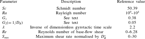
Dimensionless parameters in the present study.

The depth of the channel in the present study is chosen to be $d(\equiv 2h)=0.5~\text{cm}$ , which is comparable to that used in Durham et al. (Reference Durham, Kessler and Stocker2009) ( $d=1~\text{cm}$ ). The range of the centreline velocity $U_{c}$ tested in the present study is $U_{c}=0{-}0.25~\text{cm}~\text{s}^{-1}$ , leading to $Re=0{-}6.28$ . The onset of gyrotactic trapping is strongly linked to the base-flow vorticity at which an isolated cell will begin to tumble. For a given dimensionless gyrotactic time scale $\unicode[STIX]{x1D706}$ , such a vorticity can be calculated either in terms of the gyrotactic time scale $B$ or in terms of the rotational diffusivity $D_{R}^{\ast }$ . The critical spanwise vorticity (made dimensionless by the rotational diffusivity) at which a cell undergoing no random motion begins to tumble is $S_{crit}=4.4$ , where the spanwise vorticity of the base flow is defined as

(2.6) $$\begin{eqnarray}S(y)=-\frac{ScRe}{D_{R}^{\ast }}\frac{\text{d}U_{0}}{\text{d}y}.\end{eqnarray}$$

We note that (2.6) is useful in characterising the flow rate in relation to the cell dynamics. Using (2.6), the base-flow rate can be characterised by the maximum spanwise vorticity,

(2.7) $$\begin{eqnarray}S_{max}\equiv \max _{y}S(y),\end{eqnarray}$$

for which $S(y)=S_{max}(=2ScRe/D_{R})$ is attained at the upper wall (i.e. $y=1$ ).

All the model parameters for the individual cells in the present study (e.g. swimming speed, sedimentation speed, cell volume, etc) are those for C. nivalis. The range of the averaged cell-number density considered in the present study is $N=1\times 10^{3}{-}1\times 10^{7}~\text{cells}~\text{cm}^{-3}$ , which comfortably includes $1.1\times 10^{6}~\text{cells}~\text{cm}^{-3}$ in the experiment of Durham et al. (Reference Durham, Kessler and Stocker2009). Given the flow geometry and the parameters for the cell, this results in $Ra=10^{0}{-}10^{4}$ . All the dimensionless parameters examined in the present study are summarised in table 1.

3.1 Basic state

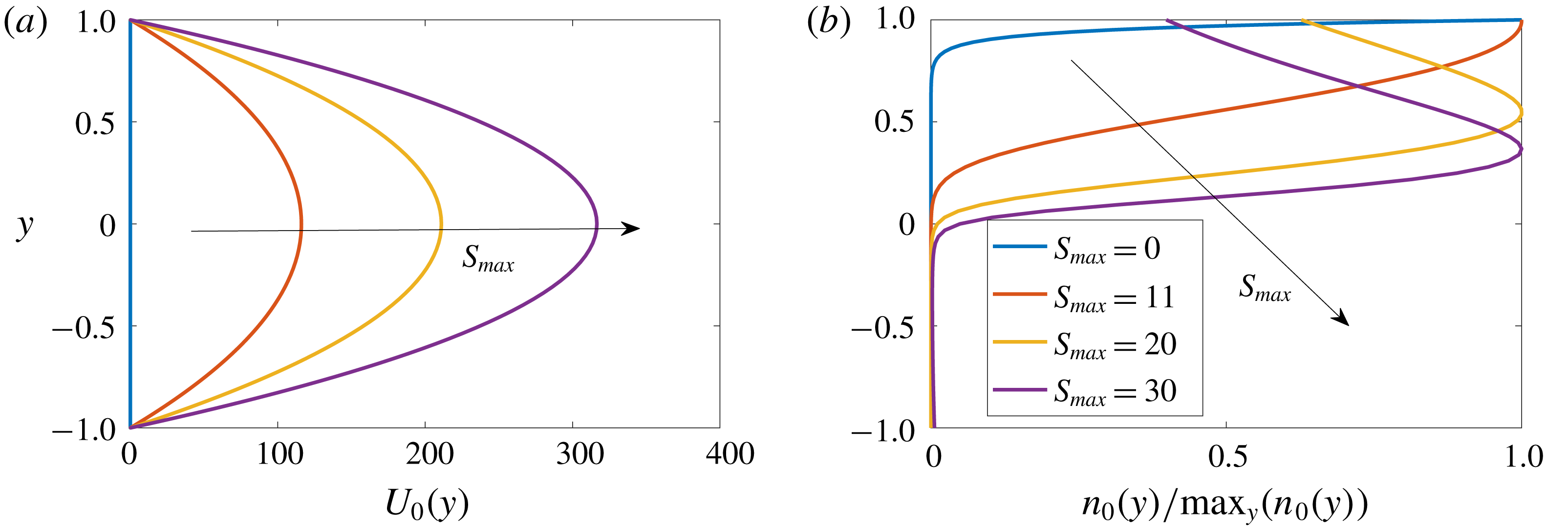
The base flow and the corresponding cell-number density distribution are plotted in figure 1(a,b), respectively. As $S_{max}$ is increased, the centreline velocity simply increases while maintaining the parabolic profile. In contrast, the profile of the cell-number density experiences non-trivial changes with the increase of $S_{max}$ . To explain this feature, we start by making a few observations. First, for a excessively large spanwise vorticity, the average upswimming speed of the cells should become smaller than the sedimentation speed, because the upswimming speed $V_{c}\langle e_{2}\rangle _{0}$ approaches zero in the limit of infinitely large vorticity (see figure 3a in Hwang & Pedley Reference Hwang and Pedley2014a ). In other words, $V_{c}\langle e_{2}\rangle _{0}\leqslant V_{s}$ for $S(y)\geqslant S_{s}$ , where $S_{s}$ is the spanwise vorticity at which $V_{c}\langle e_{2}\rangle _{0}=V_{s}$ . Note that, for the given modelling parameters, $S_{s}\simeq 11$ (figure 7 in Hwang & Pedley Reference Hwang and Pedley2014a ). Second, the form of $n_{0}(y)$ in (2.2c ) indicates that the sign of $V_{c}\langle e_{2}\rangle _{0}-V_{s}$ should be identical to that of $\text{d}n_{0}/\text{d}y$ . It follows that the peak location of $n_{0}(y)$ is identical to the location where $S(y)=S_{s}$ (or equivalently $V_{c}\langle e_{2}\rangle _{0}=V_{s}$ ), suggesting the crucial role of the sedimentation speed in the gyrotactic trapping even if it is significantly smaller than the cell-swimming speed (note that $V_{s}\simeq 0.1V_{c}$ ; see Pedley Reference Pedley2010).

Keeping these observations in mind, let us now observe $n_{0}(y)$ in figure 1(b) again. For $S_{max}=0$ , $n_{0}(y)$ is simply an exponentially growing function in the vertical direction because $\langle e_{2}\rangle _{0}$ and $D_{T0}^{22}$ in (2.2c ) are constant. When $S_{max}=11$ , $S(y=1)\simeq S_{s}$ . Therefore, $\text{d}n_{0}/\text{d}y\simeq 0$ at $y=1$ . If $S_{max}$ is increased further ( $S_{max}=20$ ), the peak location of $n_{0}(y)$ , at which $S(y)=S_{s}$ , now emerges in the region of $0<y<1$ , exhibiting an equilibrium layer of the cells formed by the gyrotactic trapping. With a further increase of $S_{max}$ , the peak location of $n_{0}(y)$ is shifted further downwards, as is shown for $S_{max}=30$ .

Figure 1.

Profiles of the basic state with $S_{max}=0,11,20,30$ : $(a)$ base flow; $(b)$ cell-number density normalised by its maximum.

3.2 Linear stability analysis

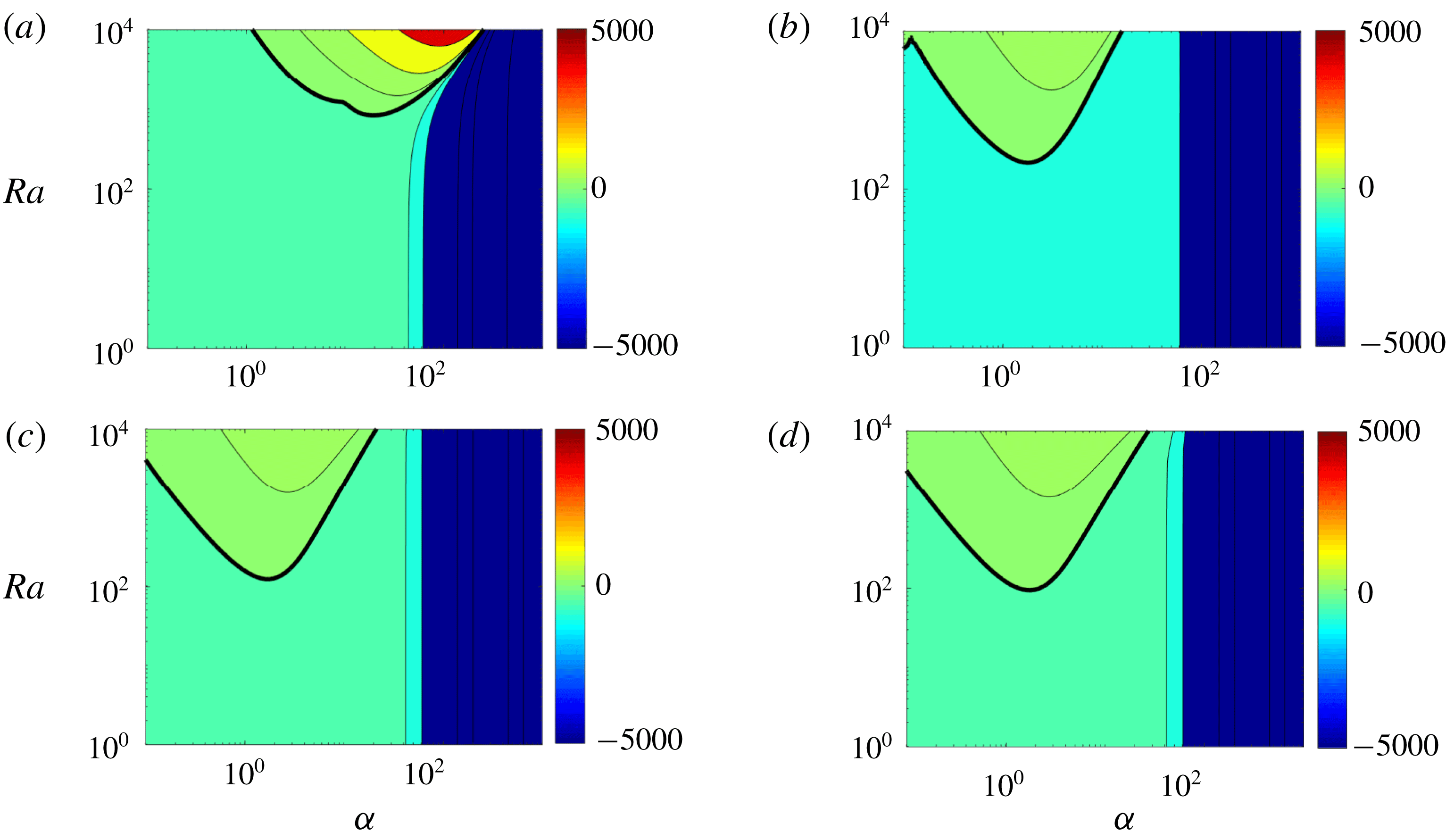
A linear stability analysis of the basic states in § 3.1 is now performed. The contours of the growth rate $\unicode[STIX]{x1D714}_{i}$ of the most unstable spanwise uniform ( $\unicode[STIX]{x1D6FD}=0$ ) mode in the $Ra{-}\unicode[STIX]{x1D6FC}$ plane are shown in figure 2 for $S_{max}=0,11,20$ and 30. For $S_{max}=0$ (figure 2 a), the neutral stability curve and the contour plot are identical to those for stationary bioconvection in Bees & Hill (Reference Bees and Hill1998) and Hwang & Pedley (Reference Hwang and Pedley2014a ). On increasing $S_{max}$ , the instabilities at high streamwise wavenumbers ( $\unicode[STIX]{x1D6FC}>20$ ) are significantly damped, while the low-wavenumber region ( $\unicode[STIX]{x1D6FC}<20$ ) is destabilised (figure 2 b–d). This tendency observed with increasing maximum base-flow vorticity is fairly similar to that in the uniform shear flow (Hwang & Pedley Reference Hwang and Pedley2014a ). However, it should be mentioned in that case, even the low-wavenumber region was also found to be completely stabilised once $S_{max}>S_{s}$ , whereas, in the present study, the region remains unstable even when $S_{max}$ is roughly three times greater than $S_{s}$ . 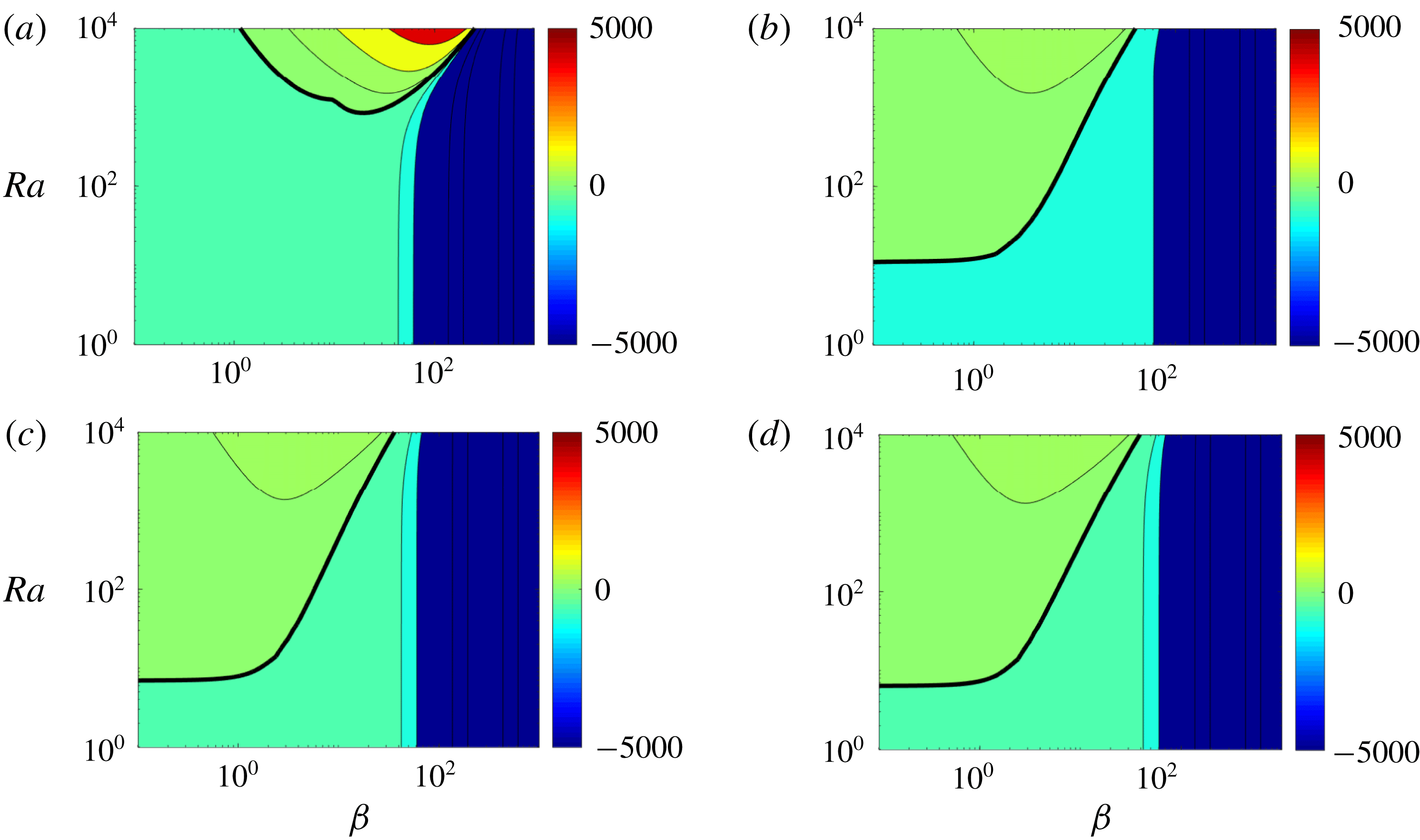Qualitatively, the same feature appears for the streamwise uniform instability mode ( $\unicode[STIX]{x1D6FC}=0$ ), as shown in figure 3. The only difference between this case and the spanwise uniform case is that the streamwise uniform mode exhibits higher growth rates at low spanwise wavenumbers ( $\unicode[STIX]{x1D6FD}<20$ ) as $S_{max}$ increases.

Figure 2.

Contours of the growth rate $\unicode[STIX]{x1D714}_{i}$ of the most unstable mode in the $Ra{-}\unicode[STIX]{x1D6FC}$ plane for $\unicode[STIX]{x1D6FD}=0$ : $(a)$ $S_{max}=0$ ; $(b)$ $S_{max}=11$ ; $(c)$ $S_{max}=20$ ; $(d)$ $S_{max}=30$ .

Figure 3.

Contours of the growth rate $\unicode[STIX]{x1D714}_{i}$ of the most unstable mode in the $Ra{-}\unicode[STIX]{x1D6FD}$ plane for $\unicode[STIX]{x1D6FC}=0$ : $(a)$ $S_{max}=0$ ; $(b)$ $S_{max}=11$ ; $(c)$ $S_{max}=20$ ; $(d)$ $S_{max}=30$ .

Figure 4.

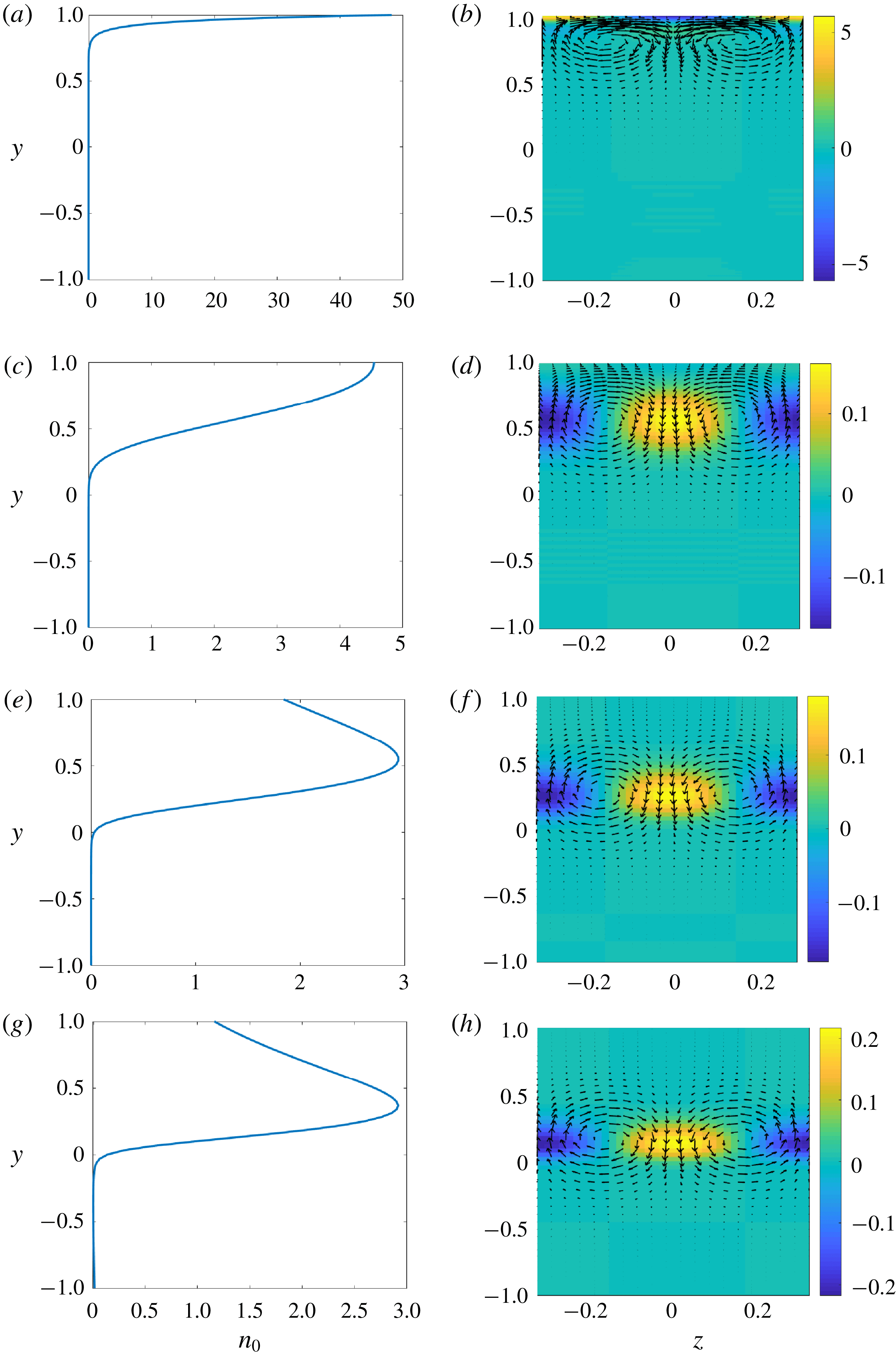
Basic-state cell-number density (a,c,e,g) and cross-streamwise view of the corresponding eigenfunction for $\unicode[STIX]{x1D6FC}=0$ , $\unicode[STIX]{x1D6FD}=10$ and $Ra=2000$ (b,d,f,h): (a,b) $S_{max}=0$ ; (c,d)  $S_{max}=11$ ; (e,f) $S_{max}=20$ ; (g,h) $S_{max}=30$ . Here, the velocity vectors show the spanwise and wall-normal velocity perturbation, and the contours indicate the perturbed cell-number density. The velocity perturbation and the perturbed cell-number density are normalised by $-\text{max}|\hat{v}||_{z=0}$ .

3.3 Physical mechanism of the instability

To understand the origin of the persistent instability, even at a considerably large base-flow vorticity, we first explore how the basic-state cell-number density profile is correlated with that of the eigenfunction of the instability mode. Figure 4 shows the basic-state cell-number density (a,c,e,g) and the cross-streamwise structure of the most unstable eigenmode (b,d,f,h) for $\unicode[STIX]{x1D6FC}=0$ , $\unicode[STIX]{x1D6FD}=10$ and $Ra=2000$ . As explained previously, the maximum $n_{0}$ , which indicates the position of the cell layer formed by the gyrotactic trapping, shifts downwards with increasing $S_{max}$ . Interestingly, the vertical location, in which the eigenmode appears in the form of counter-rotating rolls with the corresponding cell-number density field, also moves downwards together with the peak location of $n_{0}$ . Furthermore, for all $S_{max}$ considered here, the eigenmode of the instability consistently emerges in the region where the basic cell-number density is unstably stratified (i.e. $\text{d}n_{0}/\text{d}y>0$ ), suggesting that the instability would be associated with the gravitational overturning mechanism observed in Rayleigh–Bénard convection and the Rayleigh–Taylor instability.

Figure 5.

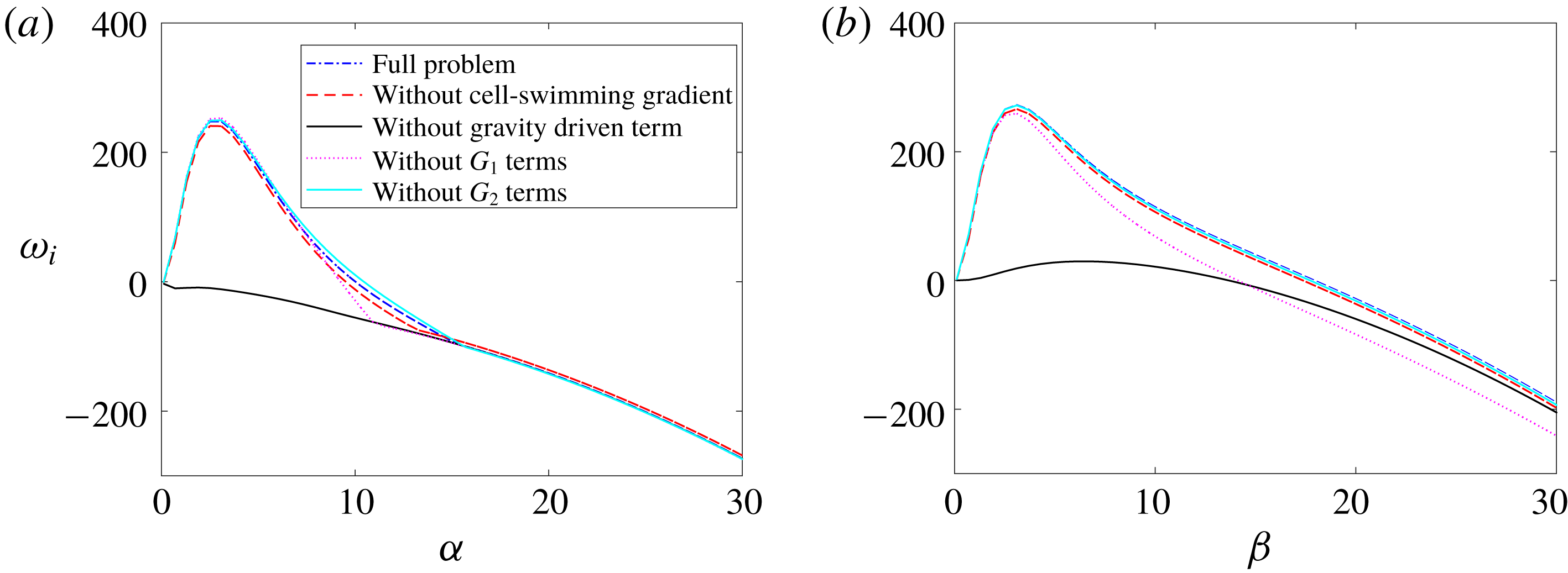
Examination of the instability mechanisms for $S_{max}=20$ and $\mathit{Ra}=2000$ : (a)  $\unicode[STIX]{x1D714}_{i}$ versus $\unicode[STIX]{x1D6FC}$ with $\unicode[STIX]{x1D6FD}=0$ ; (b)  $\unicode[STIX]{x1D714}_{i}$ versus $\unicode[STIX]{x1D6FD}$ with $\unicode[STIX]{x1D6FC}=0$ .

The precise mechanism of the instability persisting at large $S_{max}$ is further investigated by carefully examining each term of (2.5). Four different physical mechanisms of instability are identified in the present case: (1) gravitational instability ( ${\mathcal{D}}n_{0}$ in the third row of (2.5a )); (2) gyrotactic instability (all the terms with $G_{1}$ in (2.5e ) and (2.5f )); (3) diffusion-oriented instability (all the terms with $G_{2}$ in (2.5e ) and (2.5f )); (4) instability caused by the spatial gradient of cell-swimming vector field ( $V_{c}{\mathcal{D}}\langle {e_{2}}_{0}\rangle _{0}$ in (2.5d )). The first three mechanisms here were previously shown to play almost equally important roles in bioconvection instability (Hwang & Pedley Reference Hwang and Pedley2014a ), while the last one was shown to be the central mechanism for the blip instability in downward channel flow (Hwang & Pedley Reference Hwang and Pedley2014b ). Given the scope of the present study for the instability of gyrotactic trapping, here we focus on the instability emerging for $S_{max}>S_{s}$ . In such a case, the spanwise vorticity of the base flow would be fairly large in most of the vertical domain, and this yields all $\unicode[STIX]{x1D709}_{i}$ in (2.5) fairly small (the values of $\unicode[STIX]{x1D709}_{i}$ quickly diminish to zero as $S(y)\rightarrow \infty$ ; see figure 6 in Hwang & Pedley Reference Hwang and Pedley2014a ). We note that the $\unicode[STIX]{x1D709}_{i}$ appear with $G_{1}$ and $G_{2}$ throughout (2.5), indicating that the gyrotactic and diffusion-oriented mechanisms are unlikely to be very active for $S_{max}>S_{s}$ .

The discussion given above now suggests that the potential instability mechanism of the layer formed by gyrotactic trapping would originate from the gravitational mechanism and/or the one by the spatial gradient of cell-swimming vector field. To check this, we perform a numerical experiment for $Ra=2000$ and $S_{max}=20$ , in which linear stability is examined by suppressing each of the terms discussed above individually. As shown in figure 5, the dominant contribution of the instability is made by the term associated with the gravitational mechanism (i.e. ${\mathcal{D}}n_{0}$ in the third row of (2.5a )), as its suppression leads to complete stabilisation. However, the one from the spatial gradient of cell-swimming vector field is found to play no role because its suppression hardly changes the growth rate, suggesting that the dominant instability mechanism in the present study is the gravitational one.