1 Introduction
Since the 1960s, much work has been done on the capture efficiency of a cylinder perpendicular to a flow, but little has been done on angled cylinders, the focus of this study (Fuchs Reference Fuchs1964; Stechkina, Kirsch & Fuchs Reference Stechkina, Kirsch and Fuchs1969; Rodes et al. Reference Rodes, Smith, Crouse and Ramachandran1990; Espinosa-Gayosso et al. Reference Espinosa-Gayosso, Ghisalberti, Ivey and Jones2012). Total capture efficiency may be written as the sum of four separate capture methods: diffusion, interception, inertial impaction and gravitational deposition (Spielman Reference Spielman1977). For moth pheromones, the relevant regime is diffusion. However, because such a regime is difficult to study experimentally, we consider a scaled up system in which particles are captured by inertial impaction. Understanding the fluid dynamic effects of capture at the inertial regime can inspire the design of self-cleaning solar panels (Goossens, Offer & Zangvil Reference Goossens, Offer and Zangvil1993; Boyle, Flinchpaugh & Hannigan Reference Boyle, Flinchpaugh and Hannigan2015), air filters (Lee & Liu Reference Lee and Liu1982) and chemical sensors (Arshak et al. Reference Arshak, Moore, Lyons, Harris and Clifford2004).
Inertial impaction occurs when the particle’s inertia overcomes its diffusion (Wong, Ranz & Johnstone Reference Wong, Ranz and Johnstone1955). Many studies have analysed impaction due to the serious threats posed to lung health by airborne particulate matter (Zhu, Lin & Cheung Reference Zhu, Lin and Cheung2000; Chen et al. Reference Chen, Zhong, Tom, Kleinstreuer, Feng and He2016; Zhang et al. Reference Zhang, Zhang, Yi, Wang, Wang, Xu, Niu and Lin2018). Previous studies have also examined the collection efficiency at different azimuthal positions of a cylinder (Wessel & Righi Reference Wessel and Righi1988) aligned perpendicular to the flow. Particles will land on the leading edge of the cylinder at high Péclet number flow but will diffuse onto the full surface at low Péclet number. Little is known about how such behaviour changes when the cylinder or surface is tilted. Simulations have been conducted on angled solar panels intercepting ten micron dust particles. Accounting for Brownian, drag, lift, turbophoretic and gravitational forces, it has been shown that a panel angled  $30^{\circ }$ into the flow has the highest capture rate (Heydarabadi, Abdolzadeh & Lari Reference Heydarabadi, Abdolzadeh and Lari2017).
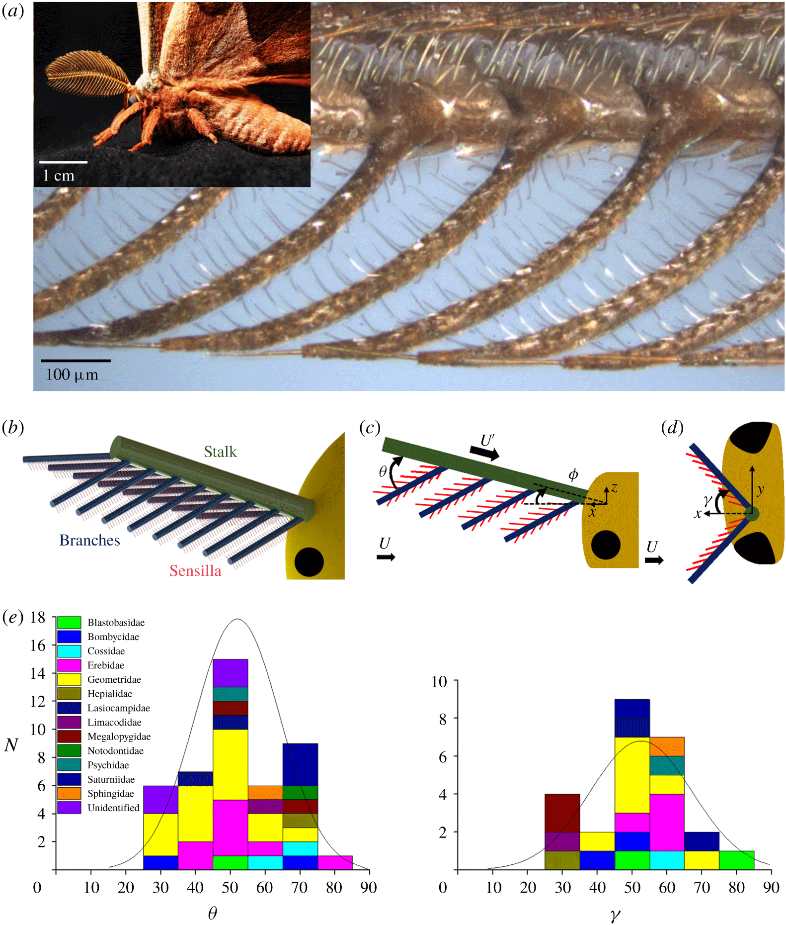
We begin our study with measurements of moth antennae, which are used to collect odour molecules. Moths have long been known as excellent chemical communicators (Karlson & Butenandt Reference Karlson and Butenandt1959; Wyatt Reference Wyatt2009). Males of many moth species track females across distances of hundreds of metres, orienting to concentrations of pheromone in parts per billion (Rau & Rau Reference Rau and Rau1929; Kuwana et al. Reference Kuwana, Nagasawa, Shimoyama and Kanzaki1999). To increase the surface area of the antenna, many lineages of male moths have enlarged, branched or doubly branched antennae, referred to here as plumose antennae. These antennae provide important mechanosensory input (Sane et al. Reference Sane, Dieudonné, Willis and Daniel2007), and have a key role in olfaction. Male moths often have large antennae relative to their body size (Schneider Reference Schneider1964); in some lineages, the antennae greatly exceed both the head and thorax in extent, as shown by the species Antheraea polyphemus in figure 1(a). Over the surface of a moth’s antennae there are chemosensilla to capture individual molecules of the female sex pheromone (Symonds, Johnson & Elgar Reference Symonds, Johnson and Elgar2012).
Moth antenna geometry. (a) Sample antenna side view image using LEXT confocal microscope. Inset image of Antheraea polyphemus with complex antennae. (b) Oblique view representation of antenna tier levels. (c) Side view schematic of antenna hierarchy levels and measured angle  $\unicode[STIX]{x1D703}$ when
 $\unicode[STIX]{x1D719}<90^{\circ }$. Black circle represents moth eye. Moth flight oriented to the left. Direction of global air velocity
 $U$ and local air velocity
 $U^{\prime }$ indicated by black arrows. (d) Top view schematic of measured
 $\unicode[STIX]{x1D6FE}$ when
 $\unicode[STIX]{x1D719}$ is
 $90^{\circ }$. Moth flight oriented to the left (only left antenna is shown). (e) Histogram of antenna branch angles
 $\unicode[STIX]{x1D703}$ (referenced to local flow direction
 $U^{\prime }$) and
 $\unicode[STIX]{x1D6FE}$ (referenced to global flow direction when
 $\unicode[STIX]{x1D719}$ is
 $90^{\circ }$). See supplementary material figure 1 available at https://doi.org/10.1017/jfm.2019.927 for discussion of sample size.

Fluid mechanical studies have been done on moth antennae but mostly focusing on the spacing between branches of the antennae rather than the angle of inclination. Antennae are believed to catch odours by a sieving action. Previous workers e.g. Koehl (Reference Koehl1994) have studied moth antennae by building enlarged models in silicone oil. At Reynolds numbers less than one, and branches with small gap to diameter ratios, antennae act like paddles. Conversely, at Reynolds numbers close to one, with large gap to diameter ratios, they act like leaky sieves (Cheer & Koehl Reference Cheer and Koehl1987b; Koehl Reference Koehl1994). Other studies have used computational modelling to study odour capture of crabs in two dimensions (Waldrop, He & Khatri Reference Waldrop, He and Khatri2018). However, experiments in water do not sufficiently account for diffusive effects, which are important for pheromones in air (Loudon & Koehl Reference Loudon and Koehl2000).
2 Results
This study involves the capture of particles of diameter  $d_{p}$ onto cylinders of diameter
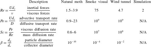
 $d_{c}$. The dimensionless groups characterizing the deposition of such particles are described in table 1 and given by
 $$\begin{eqnarray}Re=\frac{Ud_{c}}{\unicode[STIX]{x1D708}},\quad Pe=\frac{Ud_{c}}{D},\quad \unicode[STIX]{x1D6FD}=\frac{d_{p}}{d_{c}},\end{eqnarray}$$
where  $U$ is the free stream velocity,
 $\unicode[STIX]{x1D708}$ is the kinematic viscosity of air and
 $D$ is the mass diffusion coefficient of the particle or molecule in air (Crowder & Cussler Reference Crowder and Cussler1997; Huebsch Reference Huebsch2009). The Reynolds number relates the relative magnitudes of the inertial to viscous forces; the Péclet number relates the relative magnitudes of inertia to diffusion. The Schmidt number, commonly used in filtration theory (Friedlander Reference Friedlander1958), relates the viscous to diffusive force rates, and can be inferred from the Reynolds and Péclet numbers. The dimensionless length scale
 $\unicode[STIX]{x1D6FD}$ is the dimensionless particle size. In this study, we consider moth odour capture, experiments with smoke and water drops and simulations.
Reynolds numbers ( $Re$), Péclet numbers (
 $Pe$), Schmidt number (
 $Sc$) and dimensionless length scale (
 $\unicode[STIX]{x1D6FD}$) for each approach.

2.1 Moth observations
We obtained 49 North and Central American moth specimens with plumose antennae, spanning 37 species and 12 families, after capturing 300 moths from the Nantahala region of North Carolina and 24 additional moths from the University of Connecticut Insect Collection (see acknowledgements). We broke off one antenna from each moth and examined it in a three-dimensional scanning confocal microscope. A moth antenna is hierarchical, consisting of three branched tiers. From largest to smallest, these tiers are the stalk, branch and sensillum, and are coloured green, blue and red respectively in figure 1(b). The stalks we measured have a diameter of  $136\pm 36~\unicode[STIX]{x03BC}\text{m}$, comparable to that of a human hair; the branches are
 $43\pm 14~\unicode[STIX]{x03BC}\text{m}$ in diameter and are barely visible; the sensilla are
 $5.5\pm 1.4~\unicode[STIX]{x03BC}\text{m}$ and are only visible under microscopy.
We consider two possible situations associated with overall antennal posture. First, consider the stalk (in green) angled into the wind at an angle  $\unicode[STIX]{x1D719}<90^{\circ }$. Incoming air at velocity
 $U$ strikes the stalk and redirects to flow along it. The redirected velocity vector
 $U^{\prime }$ is shown in figure 1(c), where the air strikes the antenna branches held at angle
 $\unicode[STIX]{x1D703}$ with respect to the stalk. Previous literature indicates that many insects have muscular control of the tilt angle
 $\unicode[STIX]{x1D719}$ of their stalk, including hawkmoths (Krishnan et al. Reference Krishnan, Prabhakar, Sudarsan and Sane2012), locusts (Gewecke & Heinzel Reference Gewecke and Heinzel1980), honeybees (Khurana & Sane Reference Khurana and Sane2016) and cockroaches (Nishiyama, Okada & Toh Reference Nishiyama, Okada and Toh2007). Because of this muscular control, the angle of the stalk with respect to the flow is rarely measured. Nevertheless, the stalk is generally held at less than
 $90^{\circ }$ with respect to the direction of movement, as shown by cockroaches (Nishiyama et al. Reference Nishiyama, Okada and Toh2007) and bees (Sane & Jacobson Reference Sane and Jacobson2006).
If moths wish to maximize their frontal captured surface area, they may hold their antennae vertical to their head, as shown by the top view of a single antenna in figure 1(d). In this case, the air strikes the stalk perpendicularly and the air is ‘cupped’ by the branches extruding at an angle  $\unicode[STIX]{x1D6FE}$ into the flow. We do not have data on the frequency with which antennae are held in various positions, but we consider both positions for the sake of completeness. The angles
 $\unicode[STIX]{x1D703}$ and
 $\unicode[STIX]{x1D6FE}$ are independent, and therefore provide a complete geometric description for how the branches are attached to the stalk.
Previous investigators have measured by hand antenna geometry for model organisms of plumose antennae such as Bombyx mori (Vogel Reference Vogel1983), and filiform antennae of the family Heliozelidae (Wang et al. Reference Wang, Shang, Hilton, Inthavong, Zhang and Elgar2018) but made few suggestions for geometrical trends across moths. Since the angle  $\unicode[STIX]{x1D719}$ of the stalk can be adjusted by muscles at the base of the stalk, we did not measure it. Figure 1(e) shows histograms for the branching angles
 $\unicode[STIX]{x1D703}$ and
 $\unicode[STIX]{x1D6FE}$ with a normal distribution curve in black. These angles have clear optima, with averages of
 $52^{\circ }\pm 12^{\circ }$ and
 $53^{\circ }\pm 15^{\circ }$ respectively. The standard deviation is 30 % of the average, indicating a wide range and that there are diverse evolutionary pressures on moth angle as we discuss later. Nevertheless, our result suggests when a moth holds its antenna in a forward-facing or perpendicular position, the air strikes the branches at a moderate angle, between
 $40^{\circ }$ and
 $60^{\circ }$. This result is surprising because physical intuition suggests the branch angle should be
 $90^{\circ }$ in order to expose the most surface area to the wind.
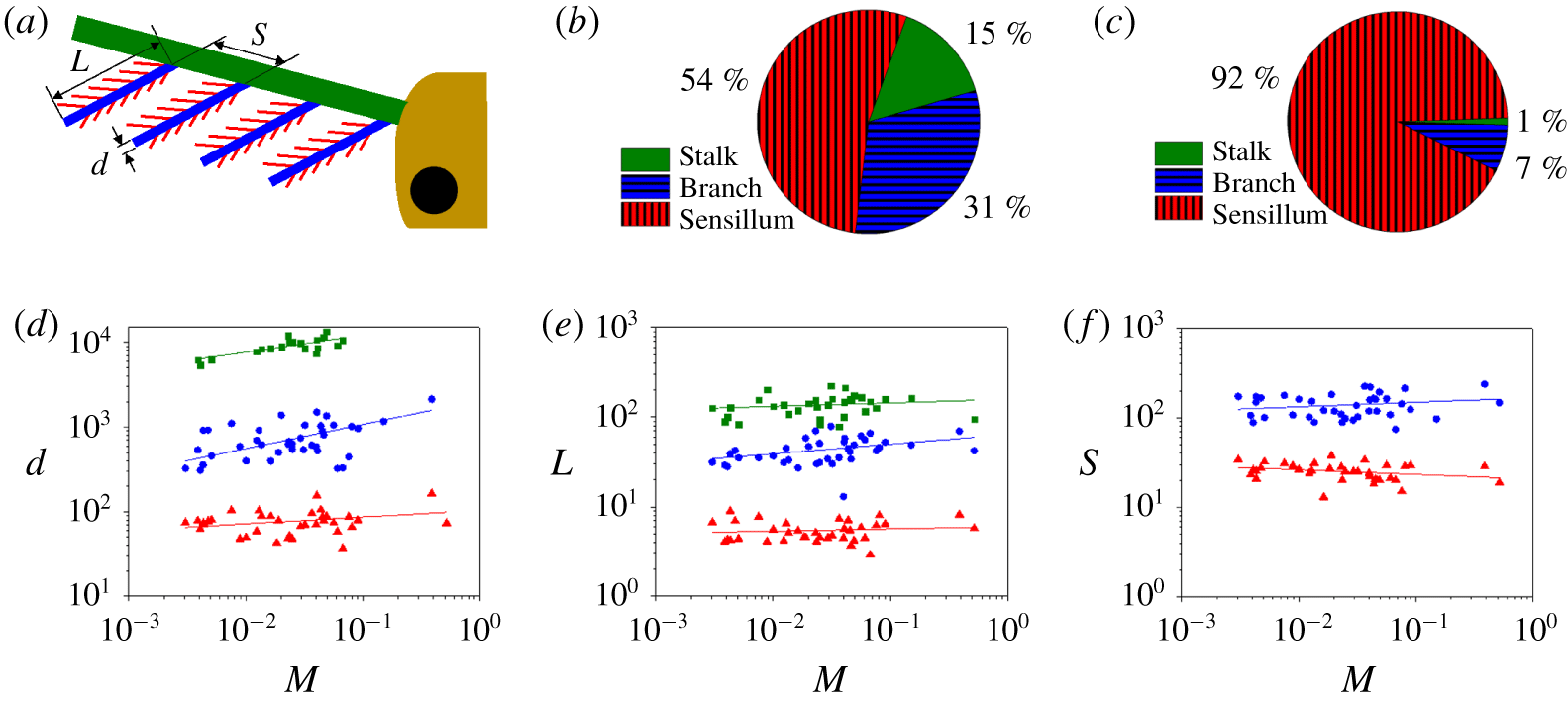
We present the dimensions of each tier of the hierarchy in figure 2. Each tier is approximately 10 times larger in length and diameter than the previous tier. The lengths and spacing of all tiers as well as the sensilla diameter are mostly constant across all moth specimens with an allometric exponent of less than 0.1, as shown in supplementary table 3. It is interesting that the diameter increases slightly with body size, possibly due to structural reasons. Estimating each tier as a cylinder, the total surface area of the average plumose antenna is found to be  ${\sim}261~\text{cm}^{2}$, the same characteristic surface area as a DVD, with the majority of the surface area distributed among the sensilla, as shown in figure 2(b). If each sensillum, branch, and stalk were to be placed end to end, the total length sums to almost one metre, as indicated by figure 2(c). Thus, a moth antenna packs a surprisingly large area and length, presumably to increase the chance of intercepting odours.
Dimensions of parts of the moth antenna. For all panels, the stalk is green, the branch is blue and the sensillum is red. (a) Schematic of the moth antenna with the length  $L$, diameter
 $d$ and spacing
 $S$ of the branches shown. (b) Distribution of surface area across the three levels of hierarchy, the stalk, branch and sensillum. (c) Distribution of length across the three levels of hierarchy, the stalk, branch and sensillum. (d) The relationship between moth mass
 $M$ (g) and diameter
 $d$ (
 $\unicode[STIX]{x03BC}\text{m}$) of the stalk, branch and sensillum. (e) The relationship between moth mass
 $M$ (g) and length
 $L$ (
 $\unicode[STIX]{x03BC}\text{m}$) of the stalk, branch and sensillum. (f) The relationship between moth mass
 $M$ (g) and spacing
 $S$ (
 $\unicode[STIX]{x03BC}\text{m}$) of the branch and sensillum. For panels (d–f), values for the stalk, branch and sensillum are represented by green squares, blue circles, and red triangles, respectively.

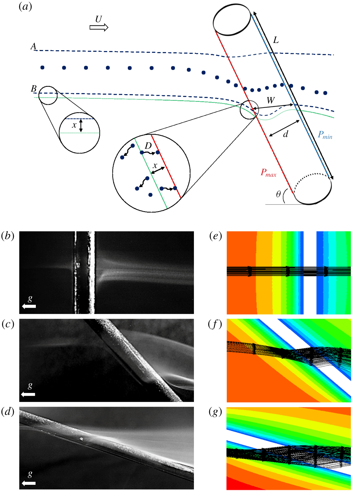
Flow around an angled cylinder. (a) Odour molecules, given by the solid blue circles, flow past an angled cylinder. The dashed blue lines denote two streamlines, marked A and B that are deformed by the influence of the cylinder. The dotted green line indicates the distance  $x$ from the cylinder that odour molecules can diffuse onto the cylinder. Once close to the cylinder, odour molecules change their path due to the pressure difference
 $P_{max}-P_{min}$ between the leading and trailing edges of the cylinders. Blue and green lines are originally aligned with the main axis of the cylinder before encountering the pressure gradient and moving around the cylinder in three-dimensional space. (b–d) Smoke rising to impact cylinders angled at
 $90^{\circ }$,
 $45^{\circ }$ and
 $15^{\circ }$ with respect to the incoming flow. Gravity
 $g$ is in the direction shown. (e–g) Simulation of flow and streamlines around
 $90^{\circ }$,
 $45^{\circ }$ and
 $10^{\circ }$ angled cylinders to flow respectively. Values range from
 $0.5~\text{m}~\text{s}^{-1}$ (red) to
 $0~\text{m}~\text{s}^{-1}$ (blue) with linear colour regression.

Using the dimensions presented in figure 2, we can determine whether neighbouring structures influence each other. A well-established criterion to determine this effect is related to the ‘leakiness’ of the structure first coined by Cheer and Koehl (Cheer & Koehl Reference Cheer and Koehl1987b). For the sensilla level, the spacing to diameter ratio is approximately 4, and the Reynolds number based on the sensillum diameter is 0.2. These parameters suggest a moderately leaky system. On the other hand, the branch level is very close to fully leaky with a spacing to diameter ratio of 3 and Reynolds number of 2. As such, the assumption of looking at a branch as an individual cylinder is much more valid than it would be at the sensillum level. We proceed by conducting smoke visualizations around a scaled-up model of a single branch of the antenna.
2.2 Smoke visualization
We perform experiments using a wooden dowel and incense particles of one micron characteristic diameter. The rising speed yields a Reynolds number of 75 and Péclet number of  $10^{9}$. Figure 3(b–d) shows the wooden dowel angled at decreasing angles with respect to the flow (
 $90^{\circ }$,
 $45^{\circ }$ and
 $15^{\circ }$). In figure 3(b), the dowel is perpendicular to the flow, and incoming smoke simply strikes the cylinder and curves around it, spreading as it does so. This phenomenon is comparable to the well-known flow past a bluff body (Munson et al. Reference Munson, Okiishi, Huebsch and Rothmayer2013). However, in figure 3(c,d), the rod is at more acute angles with the flow, a feature which changes the path of the smoke dramatically. Smoke travels down the axis of the rod before curving and going around it. This phenomenon is also shown schematically in figure 3(a): for rods angled at less than
 $90^{\circ }$ the smoke takes a compromise between the initial flow direction and a path perpendicular to the cylinder. We call this phenomenon ‘the lingering effect’ because the flow spends more time in the vicinity of the rod than in the perpendicular case. Inclining the cylinder also further decreases its frontal cross-sectional area, which in turn reduces the number of incoming streamlines that contact the cylinder. Thus, the lingering effect is strongest for moderate angles of attack.
2.3 Wind tunnel experimentation
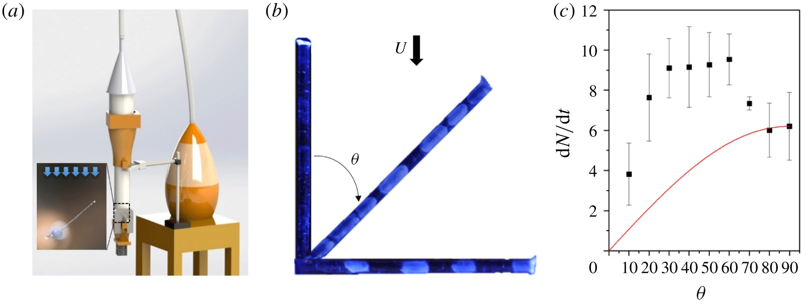
The smoke visualization gives us useful intuition on the flows generated, but to obtain quantitative information on particle deposition, we conduct wind tunnel tests. We use small plastic fibres from interdental toothbrushes, shown in figure 4. We tested three fibres at 10 increments of  $10^{\circ }$, spanning
 $0^{\circ }$,
 $10^{\circ }$,
 $20^{\circ },\ldots ,90^{\circ }$ with respect to the incoming flow. Small drops were introduced into the air stream using a humidifier containing dyed water, with the most common drop diameter of approximately
 $10~\unicode[STIX]{x03BC}\text{m}$ (Amador et al. Reference Amador, Mao, DeMercurio, Montero, Clewis, Alexeev and Hu2015). Our low-speed wind tunnel pushes air at speeds of
 $U=0.5~\text{m}~\text{s}^{-1}$, in which the associated Reynolds number based on fibre diameter
 $d_{c}$ is
 $Re=Ud_{c}/\unicode[STIX]{x1D708}=4.7$, which is close to the maximum Reynolds number of 3.9 based on the moth branch diameter and flying speed, where
 $\unicode[STIX]{x1D708}$ is the kinematic viscosity of air in both cases. The Péclet number is of the order of
 $10^{9}$, which is
 $10^{8}$ times larger than for moth olfaction, indicating that particles are predominately deposited by inertial impaction rather than diffusion.
Drop deposition on model antenna. (a) Rendering of experimental set-up with detail view of fibre in test section. (b) Dyed water agglomerated on antenna mimic at  $\unicode[STIX]{x1D703}=0^{\circ }$,
 $45^{\circ }$ and
 $90^{\circ }$ from flow direction
 $U$. (c) Particles collected in thousands per second
 $\text{d}N/\text{d}t$ after exposed to particle laden flow at varied degrees
 $\unicode[STIX]{x1D703}$. Black solid points represent mean values of experimental data with error bars of one standard deviation. Red line indicates theoretical prediction at water droplet Péclet number.

The mist agglomerates on the fibre to form larger patches visible under ultraviolet light, as shown in figure 4(b). The area of the fibre coated in fluorescence was converted to a number of drops using the image-processing described in the wind tunnel experiment methods sub-section. There was significantly less deposition at  $0^{\circ }$ and
 $90^{\circ }$, and the greatest deposition between
 $30^{\circ }$ and
 $60^{\circ }$. We use image analysis to calculate the number of drops that deposit over the duration of the experiment.
The black filled squares in figure 4(c) show the relation between the rate of drop deposition and the angle of the cylinder. At the zero degree inclination, drops simply blow past the cylinder. Deposition increases with increasing tilt angle, with a maximum collection rate of 9.5 thousand drops captured per second at  $60^{\circ }$. The rate of collection at the optimum angle is over 30 % higher than that for cylinders perpendicular to the flow. We would like to point out the similarities in the angle of highest collection rate in figure 4(c) and the most common antenna branch angle in the moth angle histograms in figure 1(e). This correspondence between the moth optima and the collection experiments is surprising because the Péclet numbers for these two cases are different by orders of magnitude. Moreover, as we shall see in our mathematical model, we do not expect an optimal deposition to occur at high Péclet number at any angle other than
 $90^{\circ }$.
In the deposition experiments, we observe a steep 20 % drop in deposition between  $60^{\circ }$ and
 $70^{\circ }$. Upon double checking the original photographs of the cylinders, we did not find any experimental artefacts that could account for this drop off. Moreover, this drop off is not present in the moth antenna angle histogram.
3 Mathematical modelling
We predict streamlines using a series of numerical simulations with the ANSYS Fluent incompressible solver and a laminar viscous model. We used a Reynolds number of 2 for our simulations. Since particles were not inserted into the flow, the Péclet number is not a relevant parameter to consider. Cylinders were angled at  $15^{\circ }$ increments relative to the bulk flow. The streamlines are shown in figure 3(e–g), and accurately recreate the paths shown in the smoke visualizations. Due to the Reynolds number of the smoke being 35 times higher than that of the simulation and flow around the moths, the smoke spreads out more than the simulation predicts, but the general shape remains consistent.
We can rationalize the distorted flow by examining the local pressure driving it. When close to the cylinder of figure 3(a), the higher pressure at the leading edge  $P_{max}$ pushes the flow in the direction perpendicular to the cylinder and towards the area of low pressure
 $P_{min}$ according to our simulations. Therefore, in the absence of any forces caused by inertia or diffusion, the particles would theoretically travel in the paths specified by the blue dotted lines A and B.
Before we begin our theoretical model, we first use our numerical ANSYS model to measure a key input parameter for our theoretical model. We define a metric  $w$ for increased path length of streamlines and which depends on the angle of the cylinder
 $\unicode[STIX]{x1D703}$. We normalize and then non-dimensionalize
 $w$ with the cylinder diameter
 $d_{c}$, creating a dimensionless
 $w^{\ast }=(w(\unicode[STIX]{x1D703})-d_{c})/d_{c}$. Defined this way,
 $w^{\ast }$ is zero if there is no increase in path length of a streamline. We measure
 $w^{\ast }$ of each angle (
 $15^{\circ }$,
 $30^{\circ }$,
 $45^{\circ }$,
 $60^{\circ }$,
 $70^{\circ }$ and
 $90^{\circ }$) from the ANSYS simulation. As shown in supplementary table 4, the values of
 $w^{\ast }$ range from
 $w^{\ast }=0$ if the cylinder is at
 $90^{\circ }$ to
 $w^{\ast }=2$ if the cylinder is at
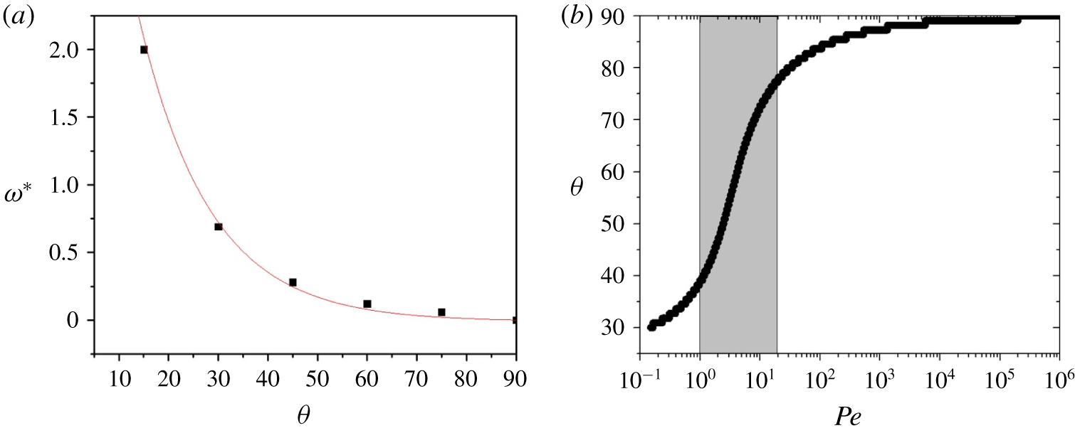
 $15^{\circ }$. We fit these trends to an exponential function using the equation
 $$\begin{eqnarray}w^{\ast }=6e^{-0.07\unicode[STIX]{x1D703}}-0.011,\end{eqnarray}$$
which is plotted in figure 5(a) and will be substituted into our theoretical model.
Increased path length values and applicable regime. (a) The  $w^{\ast }$ values from ANSYS simulation in black with exponential fit
 $w^{\ast }=6\text{e}^{-0.07\unicode[STIX]{x1D703}}-0.011$ in red. (b) Optimal capture angle
 $\unicode[STIX]{x1D703}$ at different Péclet numbers
 $Pe$ from (3.7). Shaded region indicates range for branches of moth antennae. Wind tunnel experiments operate at a higher
 $Pe$ than shown and therefore do not adhere to the proposed theory.

Although our experiments are performed at high Péclet number, it is more tractable to perform modelling for a low Péclet number regime. Classically, the efficiency  $\unicode[STIX]{x1D702}$ is dimensionless and not dependent upon the angle of orientation. Thus, the rate of particles captured by a cylinder perpendicular to the flow has been written (Palmer et al. Reference Palmer, Nepf, Pettersson and Ackerman2004; Espinosa-Gayosso et al. Reference Espinosa-Gayosso, Ghisalberti, Ivey and Jones2012) as
 $$\begin{eqnarray}\frac{\text{d}N}{\text{d}t}=\unicode[STIX]{x1D702}CUA,\end{eqnarray}$$
where  $C$ is the number of particles in the air per cubic metre and
 $U$ is the air velocity. The projected area
 $A$ of a cylinder may be written
 $A=Ld_{c}\sin \unicode[STIX]{x1D703}$ where
 $L$ and
 $d_{c}$ are the length and diameter of the cylinder, and
 $\unicode[STIX]{x1D703}$ is the angle into the flow. Equation (3.2) indicates the capture rate should be maximum if the fibre is perpendicular to the flow since that maximizes the projected area. Clearly, such a trend does not describe the angles observed. To reconcile this discrepancy, we introduce a new capture rate equation
 $$\begin{eqnarray}\frac{\text{d}N}{\text{d}t}=\unicode[STIX]{x1D6FC}\unicode[STIX]{x1D702}CUA,\end{eqnarray}$$
where we introduce a new dimensionless term  $\unicode[STIX]{x1D6FC}$ to account for the deflection of the streamlines that causes the flow to linger around the cylinder. We proceed by deriving an expression for
 $\unicode[STIX]{x1D6FC}$ by incorporating the added diffusive effects if the cylinder is angled and maintaining consistency with previous theory when predicting deposition on a perpendicular cylinder. The time
 $t$ the particle spends travelling around the cylinder is the ratio of the distance travelled
 $w^{\ast }d_{c}$ and the flow velocity
 $U$:
 $$\begin{eqnarray}t=\frac{w^{\ast }d_{c}}{U}.\end{eqnarray}$$
Since  $w^{\ast }$ increases as cylinders are tilted into the flow, so will the travel time
 $t$. This increase in time leads to an increased number of particles that reach the collector surface by diffusion. As a particle passes by the cylinder, it performs Brownian motion (Einstein Reference Einstein and Fürth1926). The distance
 $x$ a particle can travel by diffusion (Cussler Reference Cussler2009) may be written
 $$\begin{eqnarray}x=\sqrt{6Dt}.\end{eqnarray}$$
This distance  $x$ represents an incremental increase in the number of streamlines that will bring particles to impact on the cylinder. Without diffusion, the envelope remains the same. The dimensionless travel distance can be written by dividing
 $x$ by the cylinder diameter
 $d_{c}$; further combining (3.4) and (3.5), we write
 $\unicode[STIX]{x1D6FC}$ in terms of the distance
 $w^{\ast }:\unicode[STIX]{x1D6FC}=x/d_{c}+1=\sqrt{6D(w^{\ast }d_{c})/U}/d_{c}+1$. The equation can be further simplified using the Péclet number
 $Pe=Ud_{c}/D$ with the cylinder diameter as the characteristic length. Thus the equation for
 $\unicode[STIX]{x1D6FC}$ becomes
 $$\begin{eqnarray}\unicode[STIX]{x1D6FC}=\sqrt{\frac{6w^{\ast }}{Pe}}+1.\end{eqnarray}$$
Finally, combining equations (3.1), (3.3) and (3.6), the total rate of capture of particles may be written
 $$\begin{eqnarray}\frac{\text{d}N}{\text{d}t}=\left(\sqrt{\frac{36\text{e}^{-0.07\unicode[STIX]{x1D703}}-0.066}{Pe}}+1\right)\unicode[STIX]{x1D702}CULd_{c}\sin \unicode[STIX]{x1D703}.\end{eqnarray}$$
3.1 Model application
Our model is formulated in the diffusive regime, and does not show improved capture efficiency at high Péclet number. Keeping  $\unicode[STIX]{x1D702}CULd_{c}$ constant, we calculate deposition rates across angles
 $\unicode[STIX]{x1D703}$ and Péclet numbers from
 $10^{-1}$ to
 $10^{6}$, spanning both olfaction in moths and our wind tunnel experiments with drops. From each sweep, the maximum collection rate
 $\text{d}N/\text{d}t$ occurs at a different optimal angle
 $\unicode[STIX]{x1D703}$ depending on the particle diameter. As shown in figure 5(b), the optimal angle for capture is predicted to be at
 $90^{\circ }$ for high
 $Pe$ numbers but varies between
 $40^{\circ }$ and
 $75^{\circ }$ for the regime associated with moth olfaction with a branch diameter of
 $43\pm 14~\unicode[STIX]{x03BC}\text{m}$ and a diffusion coefficient of
 $2.5\times 10^{-6}~\text{m}^{2}~\text{s}^{-1}$. The disappearance of an optimal angle is consistent with the physics underlying our mathematical model. At high Péclet number, the incoming particles diffuse negligibly. Thus, there is no increase of the envelope of particles captured through the lingering effect.
As can be seen in the grey region of figure 5(b), the slope of the model line is greatest in the region corresponding to the Péclet number of moths. This sensitivity is simply due to physics, and it may have led to the large distribution of moth branch angles we observed. Of course, many other alternative hypotheses exist for this distribution. For example, the antennal branches are in all possible directions and angles, which suggests natural selection has favoured different sampling strategies in different species and environments, rather than having a single optimal angle relative to the flow. The branching angle could also have evolved to allow for better packing or due to developmental constraints. Additionally, the antennae of moths have been shown to have mechanosensory functions which could dictate that the branches make the most contact with the air possible (Sane et al. Reference Sane, Dieudonné, Willis and Daniel2007; Hinterwirth & Daniel Reference Hinterwirth and Daniel2010).
To make clear that our model cannot predict the optimal angles observed in our wind tunnel experiments, we show the predicted collection rate using the red line in figure 4(c). The value of  $\unicode[STIX]{x1D702}C$ was determined to be
 $2\times 10^{9}$ particles per
 $\text{m}^{3}$ by measuring the collection rate
 $\text{d}N/\text{d}t$ of the
 $90^{\circ }$ tests and substituting the known values into the classical (3.2). The red trend was obtained using (3.3) applied at Péclet numbers of
 $10^{9}$ with a velocity
 $U$ of
 $0.5~\text{m}~\text{s}^{-1}$, a collector length
 $L$ of
 $400~\unicode[STIX]{x03BC}\text{m}$ and a collector diameter
 $d$ of
 $135~\unicode[STIX]{x03BC}\text{m}$. Clearly the theoretical model derived for low Péclet number does not apply for higher Péclet number flow since diffusion is not the dominant method of collection.
4 Discussion
In this section, we discuss a few caveats in our modelling, biological measurements and wind tunnel experiments.
In our model, we consider only a single branch, thereby neglecting any interaction between branches. For the branch level of hierarchy, the Reynolds number is larger than one and the spacing is over  $20~\unicode[STIX]{x03BC}\text{m}$, so the Cheer and Koehl ‘leakiness’ model indicates a fully leaky system (Cheer & Koehl Reference Cheer and Koehl1987b). Therefore, Cheer and Koehl have used the Tomotika and Aoi model to describe the velocity profile around a single branch (Cheer & Koehl Reference Cheer and Koehl1987a). Our work utilizes computational tools unavailable at the time of Tomotika and Aoi but also treats each branch individually rather than as a part of a larger array. This also does not account for the sensilla protruding from the branches which could further slow the airflow and increase accumulation.
We assume the angles and lengths in dead and dried specimens to be closely approximated to those of re-hydrated individuals. In many moths, there is modest curvature of the branches. We speculate such curvature in the secondary axis of the antenna, as in figure 1(a), assures some portion of the antenna will be well situated for pheromone capture and detection.
As can be seen from the histograms in figure 1(e), there is a level of variation typical of complex biological systems. One such outlier is shown by the family Apatelodidae in black, which has a significantly smaller branch angle. This particular family of moths are colloquially called American silk moths. A similar type of silk moth has been shown to use their wings to fan the air over their antennae while stationary (Loudon & Koehl Reference Loudon and Koehl2000). Such a phenomenon could warrant future study to distinguish the different fluid mechanics while flapping in a stationary position and free flight. Other parameters such as wing flapping frequency, size and shape could also be important.
We recognize moths are complex insects with many competing constraints placed on their antennae. One constraint is the limitation of antenna size due to the increase in drag when flying. As the cross-sectional area of the antennae increases, the drag force will increase proportionally (Bishop & Hassan Reference Bishop and Hassan1964). Another consideration is evolutionary relationships among the moths studied, which is not a factor that we have considered. Additionally, the moths fly in various wind conditions and have different antenna sizes which corresponds to a range of Péclet and Reynolds numbers, as reported in table 1. The factor of 2 variation in Reynolds number across the moths sampled has a greater impact in this special regime as this indicates a factor of 2 range of inertial forces across the moth families studied. While extensive in scale, a full investigation of the observed variation could be carried out by conducting experiments directly recording the neurological signals from fresh plumose antennae from each family (Schneider, Price & Moore Reference Schneider, Price and Moore1998). If other parameters, such as overall antenna size and lure composition, could be regulated, each family of moths could also be placed in a  $y$-maze with varying concentrations to distinguish the sensing ability of each antenna structure similar to Krang et al. (Krång et al. Reference Krång, Knaden, Steck and Hansson2012).
We proceed with a few caveats regarding our experiments. In the wind tunnel experiments, all electrostatic interactions were ignored. The collector was made of nylon, which is generally neutrally or positively charged. The drops generated by the humidifier are created via a vibrating orifice aerosol generator which result in positively charged water droplets (Zilch et al. Reference Zilch, Maze, Smith, Ewing and Jarrold2008). The drops were kept at room temperature to avoid the increase in electrical potential with increased temperature (Magono & Takahashi Reference Magono and Takahashi1959). Therefore, unlike natural pollen capture (Bowker & Crenshaw Reference Bowker and Crenshaw2007), the interaction between the drops and collector should be mildly repellent without leading to an increased collection as the lingering time increases. The numerics approach did not involve particle transport and therefore did not need to include electrostatic effects. Similarly, the smoke was used only as a tracer for the velocity profile around a cylinder and as such had negligible electrostatic effect.
We made several attempts to conduct experiments at the scale of moth antennae, associated with low Péclet numbers. We created a 1 : 1 mimic of the moth antenna geometry using a NanoScribe three-dimensional printer (Spencer, Lavrik & Hu Reference Spencer, Lavrik and Hu2017), but were not able to measure the deposition of particles onto this antenna. We next used fluorescent nano-particles (Chatterjee, Gnanasammandhan & Zhang Reference Chatterjee, Gnanasammandhan and Zhang2010) which were injected into filtered air using a nebulizer (Greenspan et al. Reference Greenspan, Moss, Schleiffer and Eick1996). The air was passed through a drying chamber, differential mobility analyser (Chen et al. Reference Chen, Pui, Hummes, Fissan, Quant and Sem1998) and condensation particle counter (Kulmala et al. Reference Kulmala, Mordas, Petäjä, Grönholm, Aalto, Vehkamäki, Hienola, Herrmann, Sipilä and Riipinen2007) to determine the size distribution, shown in supplementary figure 2 with a peak size of approximately 200 nm. The fluorescent nano-particles were then captured on a small fibre angled into the flow. The fibre was rinsed in deionized water and the resulting solution was measured on a calibrated fluorescence meter. Unfortunately, the increase in fluorescence after each trial was not statistically larger than the inherent noise of the fluorescence meter’s output.
We next tried to use a cylinder (Palmer et al. Reference Palmer, Nepf, Pettersson and Ackerman2004) wrapped with pH paper to measure the deposition of ammonia vapour. As the number of hydroxide ions collected on the cylinder increases, so does the intensity of the pH paper colour change. Such colour change is recorded and calibrated (Craig et al. Reference Craig, Peterson, Nandy, Lei, Hossain, Camarena, Dodson, Cook, Dutcher and Ault2018) to obtain the number of ions collected. Unfortunately, the pH paper records orders of magnitude changes in concentration and therefore could not measure the predicted factor of two deposition among cylinders of different angle. The relationship between cylinder angle and pH change in the paper is shown in supplementary figure 3. Future workers might find these approaches useful when trying to perform deposition experiments at small Péclet numbers.
We attempted to expound upon the two-dimensional modelling methods of Waldrop et al. (Waldrop et al. Reference Waldrop, He and Khatri2018) into a three-dimensional model required for angled collection. However, the computational power available was insufficient to solve the three-dimensional model in COMSOL Multiphysics.
5 Conclusion
We began by studying the antenna branching angle of certain species of male moths that collect odour molecules at Péclet numbers of 1–20. The antenna branches have an average angle of  $52^{\circ }\pm 12^{\circ }$, which presents a sub-optimal surface area to the incoming flow. Inspired by the angles on the moth antennae, we conduct particle deposition and smoke visualization experiments with larger scale drops. Our wind tunnel experiments showed that angled cylinders at a Péclet number of
 $10^{9}$ can increase particle capture by 30 % with respect to a cylinder perpendicular to the flow. Our smoke visualizations and simulations show that angled cylinders cause streamlines to bend around cylinders, which extends their time at the cylinder surface. This lingering can cause greater deposition if the particles move to the cylinder by diffusion. Consequently, our mathematical model fails to explain the observed increased capture rate from our wind tunnel experiments at high Péclet number, where particles impact by inertia. However, our model does show that optimal capture angles exist for the Péclet number of moths, and provides one potential explanation for the prevalence of these angles in nature. We hope that the questions raised by our study will increase interest in the use of angled cylinders to capture particles.
6 Methods
6.1 Moth collection
Approximately 13 distinct species of moths were caught in the Nantahala mountain region in North Carolina. An additional 24 distinct species were obtained from various locations across North and Central America as indicated in supplementary content table 3. Moths are to be housed in the University of Connecticut Insect Collection.
6.2 Antenna imaging
One antenna was cut from its base and dry mounted onto aluminium wire with Loctite UV curing glue to allow for manipulation while imaging. A handheld UV light was then used to cure the glue and secure the antenna to the wire. The other end of the wire was inserted into a ball of modelling compound to keep the antenna from touching the microscope stage, but also to allow for easy rotation. Removing the antenna from the modelling compound resulted in accidental destruction of multiple antennae. Therefore, not all antennae used to measure  $\unicode[STIX]{x1D703}$ in figure 1(e) could be used to measure
 $\unicode[STIX]{x1D6FE}$ and vice versa.
Using an Olympus LEXT 3D Material Confocal Microscope with fixed laser wavelength of 405 nm and resolution of 120 nm results in a collapsed three-dimensional image with better resolution than standard light microscopy. An initial  $z$-stack was done with a low-powered laser for a small focal plane, to ensure angle measurements are accurate. Reflection of the laser was collected to determine the surface topography of the object being imaged. The same sliced
 $z$-stack was re-imaged using light microscopy using the points which were previously determined to be on the surface of the object. In this way a high-resolution two-dimensional image was created from a small three-dimensional object. A sample image using this technique can be found in figure 1(a). Analysis of antennae was done using a custom MATLAB code which determines the angle between the stalk and the branches on it. Two vectors are defined by user input (clicking points on the screen) to calculate the angle.
6.3 Antenna dimensions
All length measurements were completed using ImageJ image processing (Schneider, Rasband & Eliceiri Reference Schneider, Rasband and Eliceiri2012). The estimated surface area  $A_{s}$ was calculated according to
 $A_{s}=\unicode[STIX]{x03C0}(L_{st}d_{st}+N_{b}L_{b}d_{b}+N_{s}L_{s}d_{s})$ where
 $L_{st}$ is the length of one stalk,
 $d_{st}$ is the stalk diameter,
 $N_{b}$ is the number of branches,
 $L_{b}$ is the length of one branch,
 $d_{b}$ is the branch diameter,
 $N_{s}$ is the number of sensilla,
 $L_{s}$ is the length of one sensillum and
 $d_{s}$ is the sensilla diameter. The total number of branches
 $N^{b}$ and sensilla
 $N^{s}$ were not individually counted but rather estimated using the centre to centre spacing according to
 $N_{b}=L_{st}/S_{b}$ and
 $N_{s}=N_{b}(L_{b}/S_{s})$.
6.4 Simulation method
To investigate flow through the antenna branch, the antenna is simplified to a cylinder model. At the local Reynolds number  $Re=Ud_{c}/\unicode[STIX]{x1D708}=1$, where
 $U$ is the incoming air velocity and
 $\unicode[STIX]{x1D708}$ is the kinematic viscosity of air (property at 293 K and 1 atmosphere), we obtain laminar flow by solving the Navier–Stokes equations, using ANSYS Fluent incompressible solver and a laminar viscous model. Numerical solution methods include: SIMPLEC pressure–velocity coupling method, least squares cell based spatial discretization for the gradient, second-order spatial discretization for pressure, second-order upwind spatial discretization for momentum. The residual convergence criterion is approximately
 $10^{-6}$.
The simulations are conducted in a rectangular domain. The domain has dimensions  $20\times 20\times 20$ times the cylinder diameter, and the cylinder has a length of 16 times the cylinder diameter. This domain is discretized by a tetrahedral unstructured grid with a minimum grid dimension of 0.1 times the cylinder diameter. Mesh resolution is validated by an independence check. The surrounding fluid domain size is increased until the change in outer boundary size no longer affects the flow around the cylinder.
6.5 Wind tunnel experiment
An antenna branch mimic was created using a hydrophilic nylon fibre removed from a size 9 Pixter interdental brush with a length of 4 mm and diameter of 0.135 mm. A wind tunnel apparatus was constructed using a three-dimensionally printed collector and diffuser, drinking straws for the straightener, a clear PVC tube for the working section and a computer fan to pull the air through the tunnel. The air speed was kept at approximately  $0.5~\text{m}~\text{s}^{-1}$ to ensure the Reynolds number stayed at approximately 4.6 using the fibre diameter as the reference length. The fibre was placed in the test section of the wind tunnel at an angle with respect to the flow from
 $0^{\circ }{-}90^{\circ }$ in increments of
 $10^{\circ }$ per test. At the inlet of the wind tunnel, 5 micron in radius drops of dyed water were generated using a Crane model ultrasonic humidifier in a similar experimental set-up to Amador et al. (Reference Amador, Mao, DeMercurio, Montero, Clewis, Alexeev and Hu2015). The dyed water consisted of 6 mg Acridine Orange per ml of water.
The characterization of the drops’ size was done using an electrostatic classifier 3080, differential mobility analyser 3081 and a condensation particle counter 3785 by TSI Inc. The time per scan is 120 s, particle size from 7 to 300 nm, with 103 channels and a lognormal fit (Seinfeld Reference Seinfeld and Mucignat-Caretta2006).
After being subjected to the particle infused flow for one minute, the wind tunnel was turned off. The fibre was imaged with a dissection microscope at  $4\times$ magnification under UV light with the axis of the fibre perpendicular to the viewing angle. The fibre was then cleaned and allowed to dry before the experiment was repeated. Deposition area measurements were obtained using an image analysis MATLAB code which traces the fluorescent area on each fibre. Because the agglomerations are located along the central axis of the fibre, the effects of curvature in the area calculations were considered negligible. The percentage of the fibre surface area coated with fluorescence after the one minute trial was then divided by 60 to get the percentage
 $\unicode[STIX]{x1D705}$ covered per second. To convert to the rate of particles captured per second
 $\text{d}N/\text{d}t$, the percentage covered per second
 $\unicode[STIX]{x1D705}$ was multiplied by the ratio of the fibre’s surface area disregarding the end caps
 $\unicode[STIX]{x03C0}d_{c}L$ and divided by the cross-sectional area of one particle
 $\unicode[STIX]{x03C0}r_{p}^{2}$ according to the equation
 $\text{d}N/\text{d}t=\unicode[STIX]{x1D705}d_{c}L/r_{p}^{2}$ where
 $d_{c}$ is the fibre diameter,
 $L$ is the fibre length and
 $r_{p}$ is the peak drop radius. For example, when the fibre is held at
 $90^{\circ }$ into the flow for one minute there is 23 % of the fibre covered, leading to a
 $\unicode[STIX]{x1D705}$ of
 $23/60$. With a fibre diameter
 $d_{c}$ of
 $135~\unicode[STIX]{x03BC}\text{m}$, a fibre length
 $L$ of 3 mm and a drop radius
 $r_{p}$ of
 $5~\unicode[STIX]{x03BC}\text{m}$, the resulting capture rate is 6.2 thousand particles per second.
Acknowledgements
This material is based upon work supported by the National Science Foundation Graduate Research Fellowship and the National Science Foundation grant no. 1510884. For specimens and comments on early drafts of the manuscript, we thank D. Wagner at the University of Connecticut, R. Weber for particle size characterization, as well as M. Ballard, P. Yeh and M. Matherne for their early contributions.
Declaration of interests
The authors report no conflict of interest.
Supplementary material
Supplementary material is available at https://doi.org/10.1017/jfm.2019.927.