





1 Introduction
Fluid filled bodies showing longitudinal libration, that is, a sinusoidal modulation of the background rotation rate, are common in the astrophysical context but form also an interesting set-up for engineering applications. Of particular interest is the question what kind of mean flows can be driven by the libration and hence a number of recent studies have focused on this problem (Noir et al.
Reference Noir, Hemmerlin, Wicht, Baca and Aurnou2009, Reference Noir, Calkins, Lasbleis, Cantwell and Aurnou2010; Calkins et al.
Reference Calkins, Noir, Eldredge and Aurnou2010; Busse Reference Busse2011; Lopez & Marques Reference Lopez and Marques2011; Sauret et al.
Reference Sauret, Cébron, Le Bars and Le Dizès2012; Klein et al.
Reference Klein, Seelig, Kurgansky, Ghasemi, Borcia, Will, Schaller, Egbers and Harlander2014; Ghasemi et al.
Reference Ghasemi, Klein, Harlander, Kurgansky, Schaller and Will2016; Hoff, Harlander & Triana Reference Hoff, Harlander and Triana2016). Simply speaking, for a cylindrical cavity in the limit when the libration frequency is small in comparison with the rotation rate
 $\unicode[STIX]{x1D6FA}_{0}$
, but large in comparison with the inverse of the spin-up time, the mean flow is a retrograde solid body rotation (Busse Reference Busse2011). The reason for the mean flow is a nonlinear self-interaction of the laminar oscillating flow in the Ekman boundary layer (already described by Wang Reference Wang1970), neglecting the effects in the Stokes boundary layer parallel to the rotation axis which is usually considered to be less important. Similar results could be found for a spherical cavity (Busse Reference Busse2010).
From a physical and mathematical point of view, rotating axial boundary layers are less well studied than Ekman boundary layers since their analytical treatment is more complicated (Chemin et al. Reference Chemin, Desjardins, Gallagher and Grenier2006). In fact, also for the problem of a librating rotating cylinder they can become very important. Noir et al. (Reference Noir, Hemmerlin, Wicht, Baca and Aurnou2009) realized that for moderate libration amplitude in a weakly nonlinear flow regime Görtler vortices can form in the centrifugally unstable Stokes boundary layer. Just recently Ghasemi et al. (Reference Ghasemi, Klein, Harlander, Kurgansky, Schaller and Will2016) suggest that these vortices can transport angular momentum away from the near-wall region into the bulk, inducing a mean flow there. These authors showed that when the boundary layer becomes unstable the vortices drive a retrograde (prograde) mean flow close to the librating outer (inner) wall. This can be seen as an inverse cascade and the responsible mechanism can be characterized as angular momentum pumping from the boundary layer into the bulk by the small-scale Görtler vortices. The strength of the excited mean flow is of the same order as the mean flow induced by nonlinear effects in the oscillating Ekman boundary layer. The generation of Görtler vortices in the equatorial region of a spherical shell has been reported by Calkins et al. (Reference Calkins, Noir, Eldredge and Aurnou2010) and by Sauret, Cébron & Le Bars (Reference Sauret, Cébron and Le Bars2013). However, for this geometry it is not clear how much this instability of the boundary layer contributes to the mean flow.
For cylindrical geometries with the axis of symmetry aligned with the axis of rotation, all boundary layers are either horizontal or axial. For a sphere, however, the boundaries have all directions so that features of the Stokes and the Ekman boundary layers might likewise be present. When Ekman boundary layers become axial they degenerate into another type of boundary layer, a process called equatorial degeneracy. Hence, as pointed out by Chemin et al. (Reference Chemin, Desjardins, Gallagher and Grenier2006), for the spherical shell geometry, questions related to the formation of boundary layers are widely open. It is thus worth to look for simpler geometries that still cover certain aspects of the spherical shell geometry.
One example of such a simplification was introduced by Busse & Or (Reference Busse and Or1986). They used an annular geometry to study thermal convection in rotating systems motivated by planetary problems. To include the
 $\unicode[STIX]{x1D6FD}$
-effect (i.e. the effect of Earth’s curvature), the top and bottom end boundaries were conical such that the depth of the fluid in the direction of the axis of rotation varied with the distance from the axis. Another example for a simplified geometry is the one studied by Klein et al. (Reference Klein, Seelig, Kurgansky, Ghasemi, Borcia, Will, Schaller, Egbers and Harlander2014). These authors also used an annular geometry but the inner wall was a cone and not a straight cylinder to mimic curvature. (The cone resembles the local inclination of a spherical wall.) Klein et al. (Reference Klein, Seelig, Kurgansky, Ghasemi, Borcia, Will, Schaller, Egbers and Harlander2014) investigated the excitation of inertial waves by librating the outer cylinder together with the end plates or the inner cone. They found that the critical angle of the slope determines the frequency of the most efficient wave excitation. Similar experiments have been done for the spherical shell geometry (Koch et al.
Reference Koch, Harlander, Egbers and Hollerbach2013; Hoff et al.
Reference Hoff, Harlander and Triana2016). Note that since the main interest of the present study is the development of Görtler vortices, their interactions with the boundary layer and the bulk flow, approximations like the small-gap limit are not useful. By neglecting curvature in the small-gap limit the Görtler instability would be suppressed and we would exclude the kind of instability we want to study. Moreover, for many applications the gap width is large, for example for geophysically motivated problems like the dynamics of planetary fluid cores, the radius ratio is approximately
 $1/3$
. Compared to small-gap flows, the wide-gap situation is more challenging, however, it can be tackled by direct numerical simulation (DNS). On the other hand, the stable laminar structure of the Ekman–Stokes boundary layer (ESBL) can be studied without including curvature in the axial–radial section by formulating a simple sloping
 $f$
-plane model (see § 3.1 and also Salon & Armenio (Reference Salon and Armenio2011)).
In the present paper we reconsider the previous study by Ghasemi et al. (Reference Ghasemi, Klein, Harlander, Kurgansky, Schaller and Will2016) but use the same geometry as used by Klein et al. (Reference Klein, Seelig, Kurgansky, Ghasemi, Borcia, Will, Schaller, Egbers and Harlander2014), that is, replace the inner cylinder by a cone. In that geometry, the boundary layer along the sloping wall is neither a pure oscillating Ekman nor a pure rotating Stokes boundary layer but the properties of both boundary layers characterize the flow. This is similar to the spherical shell where the boundary layer along the inner sphere has any orientation with respect to the rotation axis and thus possesses, over the major part of the sphere, properties of the Ekman and Stokes boundary layers. One of our main results is that for cone angles above a critical value (i.e. weak slopes) the instability is suppressed and no Görtler vortices can form. The reason is that the Reynolds stress term formed by the axial and azimuthal flow component, not present for the geometry with an axial inner cylinder, becomes important. This term is a destructing agent that controls the terms that imply the angular momentum transport into the bulk and hence the mean flow. However, for large cone angles (i.e. weak slopes), a mean flow can be excited by nonlinear effects of the oscillating Ekman boundary layer as described by Busse (Reference Busse2010) and others.
The rest of this paper is organized as follows. In § 2 we briefly describe the mathematical formulation and the numerical model. A more complete description of the model can be found in Klein et al. (Reference Klein, Seelig, Kurgansky, Ghasemi, Borcia, Will, Schaller, Egbers and Harlander2014), Klein (Reference Klein2016). In § 3 we discuss the properties of the sloping boundary layer (denoted here as Ekman–Stokes boundary layer) with the aid of laminar boundary layer theory and DNS. We do this first for stable and then for unstable flow conditions. After that, we investigate the boundary layer instability in terms of the orientation of Görtler vortices as a function of the inclination angle of the conical inner wall. This is used to infer the mean flow generation mechanism in the case of an unstable boundary layer. Then, by computing the size of the different terms in a diagnostic Reynolds-averaged Navier–Stokes (RANS) equation, we clarify the process that suppresses the mean flow excitation for super-critical cone angles. Finally, in § 4 we summarize our results and give conclusions.
2 Method
2.1 The librating annulus configuration
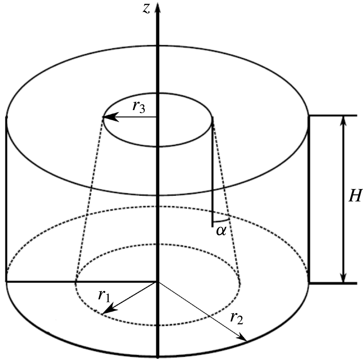
Schematic drawing of the annular configuration investigated. The inner wall is a truncated cone (frustum) with apex half-angle
 $\unicode[STIX]{x1D6FC}$
, which is likewise the inclination angle towards the symmetry axis. The set-up revolves around its symmetry axis
 $\boldsymbol{e}_{z}$
with constant mean angular velocity. Flows are excited by modulating the rotation frequency of the frustum (so-called longitudinal libration). In the present study
 $\unicode[STIX]{x1D6FC}$
is varied in small steps from
 $0^{\circ }$
to
 $18^{\circ }$
(see table 1 for details).
We study the flow of an incompressible, homogeneous, Newtonian fluid with the kinematic viscosity
 $\unicode[STIX]{x1D708}$
in various annular confinements possessing different frustum inclination angles
 $\unicode[STIX]{x1D6FC}$
. All configurations are comparable to that sketched in figure 1. Such cylindrical geometries have been studied in the past (e.g. Henderson & Aldridge Reference Henderson and Aldridge1992) and recently (Klein et al.
Reference Klein, Seelig, Kurgansky, Ghasemi, Borcia, Will, Schaller, Egbers and Harlander2014, e.g.). In the present work we use the same configuration and parameters as in Klein et al. (Reference Klein, Seelig, Kurgansky, Ghasemi, Borcia, Will, Schaller, Egbers and Harlander2014), though in contrast to these authors we do not compare numerical and experimental results. Nevertheless, the numerically extracted data form an ideal basis for future experiments to test the findings but also to extend them to cases with smaller Ekman numbers. It has been emphasized that annular confinements with inner truncated cones cover some essential aspects of a spherical shell geometry. These are, for example, sloping
 $f$
-plane effects (where
 $f$
is the Coriolis parameter) (e.g. Pedlosky Reference Pedlosky1987), critical latitudes and boundary layer eruptions. In the cylindrical configuration, the notorious complexity of a spherical set-up has been reduced by limiting our attention to a single inclination angle
 $\unicode[STIX]{x1D6FC}$
rather than the interval
 $0\leqslant |\unicode[STIX]{x1D6FC}|\leqslant \unicode[STIX]{x03C0}/2$
. The important consequence is that any breakdown of the Ekman layer has been removed on purpose from the dynamics while sloping
 $f$
-plane effects are maintained. Note, however, that it is possible to simulate precisely the breakdown condition by selecting the wall inclination and libration frequency appropriately (see Klein et al.
Reference Klein, Seelig, Kurgansky, Ghasemi, Borcia, Will, Schaller, Egbers and Harlander2014).
The annular confinement shown in figure 1 consists of a truncated cone (so-called frustum) on the inside with a maximum radius
 $r_{1}$
at the bottom (
 $z=0$
) and minimum radius
 $r_{3}(\unicode[STIX]{x1D6FC})\leqslant r_{1}$
at the top (
 $z=H$
), a straight cylinder of radius
 $r_{2}$
on the outside and rigid lids at the bottom and at the top. We consider variations of the inclination angle
 $\unicode[STIX]{x1D6FC}$
and keep all radii at the bottom (
 $z=0$
) fixed. The frustum radius
 $R(z;\unicode[STIX]{x1D6FC})$
and the annulus gap width
 $\unicode[STIX]{x0394}r(z;\unicode[STIX]{x1D6FC})$
depend on the height
 $H$
and the cone angle
 $\unicode[STIX]{x1D6FC}$
. They are given by
 $$\begin{eqnarray}\displaystyle R(z;\unicode[STIX]{x1D6FC})=r_{1}-z\tan \unicode[STIX]{x1D6FC}\quad \text{and}\quad \unicode[STIX]{x0394}r(z;\unicode[STIX]{x1D6FC})=r_{2}-R(z;\unicode[STIX]{x1D6FC}). & & \displaystyle\end{eqnarray}$$
One has
 $R=r_{1}$
at the bottom and
 $R=r_{3}=r_{1}-H\tan \unicode[STIX]{x1D6FC}$
at the top. The constraint
 $r_{3}>0$
limits the maximum cone angle that can be reached for a given radius-to-height ratio
 $r_{1}/H$
.
Seven different geometries (denoted
 $G1$
–
 $G7$
) have been investigated by varying the cone angle
 $\unicode[STIX]{x1D6FC}$
in the range
 $[0^{\circ },18^{\circ }]$
in steps of
 $3^{\circ }$
(see table 1). For
 $\unicode[STIX]{x1D6FC}=0^{\circ }$
(
 $G1$
) a standard Taylor–Couette configuration is realized in which a straight inner cylinder is coaxially aligned with the outer cylinder. For the present study we adopted a wide-gap configuration to allow for a wide range of accessible wall inclination angles. Using
 $r_{1}$
as length scale, the geometries investigated are characterized by the dimensionless values
 $r_{1}=1$
,
 $r_{2}=1.4$
and
 $H=1.5$
. For the case of
 $\unicode[STIX]{x1D6FC}=0^{\circ }$
, this corresponds also to the often-used radius ratio
 $r_{1}/r_{2}\approx 0.72$
(e.g. Czarny & Lueptow Reference Czarny and Lueptow2007; Paoletti & Lathrop Reference Paoletti and Lathrop2011; Avila Reference Avila2012; Ostilla-Mónico et al.
Reference Ostilla-Mónico, van der Poel, Verzicco, Grossmann and Lohse2014; Nordsiek et al.
Reference Nordsiek, Huisman, van der Veen, Sun, Lohse and Lathrop2015). The aspect ratio considered here is
 $\unicode[STIX]{x1D6E4}=H/(r_{2}-r_{1})=3.75$
, which is rather small but necessary to accommodate a broad range of inclination angles. In addition, the small aspect ratio helps to make three-dimensional (3-D) DNS feasible.
Details of the configurations
 $G1$
–
 $G7$
investigated by varying the cone angle
 $\unicode[STIX]{x1D6FC}$
. Corresponding values of the effective Coriolis parameter
 $f_{\ast }$
(as multiple of the mean rotation rate) and the time scale ratio
 $\unicode[STIX]{x1D6FE}$
are given. The boundary layer thickness
 $\unicode[STIX]{x1D6FF}$
equals to
 $\unicode[STIX]{x1D6FF}_{-}$
for
 $G2$
–
 $G7$
(ESBL), but
 $\unicode[STIX]{x1D6FF}_{S}$
for
 $G1$
(SBL).
 $N_{r}$
,
 $N_{z}$
,
 $N_{\unicode[STIX]{x1D703}}$
denote the number of grid points used in the radial, axial and azimuthal directions. The high-resolution cases are printed in bold. The minimum and maximum grid spacing
 $\unicode[STIX]{x0394}r_{min}$
and
 $\unicode[STIX]{x0394}r_{max}$
is given for the radial direction. The grid spacing along the sloping wall is almost equidistant with
 $\unicode[STIX]{x0394}_{z}\approx 3.5\times 10^{-3}$
. The boundary layer thickness
 $\unicode[STIX]{x1D6FF}$
is approximately resolved for the geometries
 $G1$
and
 $G2$
with nine grid cells, and for the other geometries with more than ten grid cells.

Initially, we assume the whole system to be in uniform rotation (angular velocity
 $\unicode[STIX]{x1D6FA}_{0}\boldsymbol{e}_{z}$
) around its axis of symmetry. Flows relative to this state of rigid body rotation are excited by longitudinal libration of the inner boundary. That is, the rotation rate of the inclined inner wall is subject to sinusoidal modulations of the form
 $$\begin{eqnarray}\displaystyle \unicode[STIX]{x1D6FA}(t)=\unicode[STIX]{x1D6FA}_{0}[1+\unicode[STIX]{x1D700}\sin (\unicode[STIX]{x1D714}t)] & & \displaystyle\end{eqnarray}$$
in which
 $\unicode[STIX]{x1D700}$
is the (dimensionless) libration amplitude and
 $\unicode[STIX]{x1D714}$
is the libration frequency. The libration amplitude gives rise to a local perturbation velocity
 $\unicode[STIX]{x1D700}\unicode[STIX]{x1D6FA}_{0}R(z;\unicode[STIX]{x1D6FC})$
, which is of the order
 $\unicode[STIX]{x1D700}\unicode[STIX]{x1D6FA}_{0}r_{1}$
for a small cone angle and an aspect ratio of order one. The cone angle does not notably affect the velocity scale, but will affect the local Coriolis (i.e.
 $f$
-plane effect) which will be discussed further in § 3.1 below.
2.2 Governing equations
We are interested in small-amplitude flows relative to the background rigid body rotation
 $\unicode[STIX]{x1D6FA}_{0}$
. A perturbation is prescribed by longitudinal libration of the frustum. The perturbation propagates away from the wall due to viscous diffusion. At finite distance from the wall the perturbation velocity will then be subject to the Coriolis force and nonlinearity so that instabilities may develop. The equations of motion describing this flow are given by the incompressible Navier–Stokes equations in the co-rotating frame of reference,
 $$\begin{eqnarray}\displaystyle & \displaystyle \frac{\unicode[STIX]{x2202}\boldsymbol{u}}{\unicode[STIX]{x2202}t}+Ro(\boldsymbol{u}\boldsymbol{\cdot }\unicode[STIX]{x1D735})\boldsymbol{u}+2\boldsymbol{e}_{z}\times \boldsymbol{u}=-\unicode[STIX]{x1D735}\unicode[STIX]{x1D719}-E\unicode[STIX]{x1D735}\times (\unicode[STIX]{x1D735}\times \boldsymbol{u}), & \displaystyle\end{eqnarray}$$
 $$\begin{eqnarray}\displaystyle & \displaystyle \unicode[STIX]{x1D735}\boldsymbol{\cdot }\boldsymbol{u}=0, & \displaystyle\end{eqnarray}$$
where
 $\boldsymbol{u}$
is the velocity,
 $\unicode[STIX]{x1D719}$
is the fluctuating kinematic pressure,
 $t$
is the time,
 $\unicode[STIX]{x1D735}$
is the nabla operator,
 $Ro$
is the Rossby number and
 $E$
is the Ekman number. The rotational form of the viscous diffusion term is used to highlight the importance of the vorticity
 $\unicode[STIX]{x1D735}\times \boldsymbol{u}$
for three-dimensional flows.
Equations (2.3) and (2.4) were made dimensionless by taking the maximum radius of the librating wall as length scale (
 $L=r_{1}$
), the wall libration as velocity scale (
 $U=\unicode[STIX]{x1D700}\unicode[STIX]{x1D6FA}_{0}r_{1}$
) and the mean rotation rate as inverse time scale (
 $T=\unicode[STIX]{x1D6FA}_{0}^{-1}$
). The acceleration terms are normalized with
 $\unicode[STIX]{x1D700}\unicode[STIX]{x1D6FA}_{0}^{2}r_{1}$
. This yields two dimensionless control parameters in (2.3): the Rossby number
 $Ro$
and the Ekman number
 $E$
given by
 $$\begin{eqnarray}\displaystyle Ro=\frac{U}{r_{1}\unicode[STIX]{x1D6FA}_{0}}=\unicode[STIX]{x1D700}\quad \text{and}\quad E=\frac{\unicode[STIX]{x1D708}}{\unicode[STIX]{x1D6FA}_{0}r_{1}^{2}}. & & \displaystyle\end{eqnarray}$$
The Rossby number measures the strength of the nonlinear momentum advection relative to the Coriolis force and is in the present scaling equal to the libration amplitude
 $\unicode[STIX]{x1D700}$
. The Ekman number measures the strength of viscous forces relative to the Coriolis force. Both are measures for the integral scale of the flow so that the bulk Reynolds number estimated for system-scale motions is given by
 $Re=Ro/E$
.
We seek solutions to the governing (2.3) and (2.4) in terms of the velocity field
 $\boldsymbol{u}(\boldsymbol{x},t)$
subject to the no-slip boundary condition at the domain boundary. In the co-rotating frame of reference (rotating with
 $\unicode[STIX]{x1D6FA}_{0}$
) and with respect to cylindrical coordinates, the velocity boundary conditions complementing the dimensionless equations of motion are given by
 $$\begin{eqnarray}\displaystyle u_{r}=u_{z}=0\quad \text{and}\quad u_{\unicode[STIX]{x1D703}}=\left\{\begin{array}{@{}ll@{}}r\sin (\unicode[STIX]{x1D714}t) & \text{at }r=R(z;\unicode[STIX]{x1D6FC}),\\ 0 & \text{otherwise},\end{array}\right. & & \displaystyle\end{eqnarray}$$
where
 $R(z;\unicode[STIX]{x1D6FC})$
is given by (2.1). The first expression for the radial velocity
 $u_{r}$
and the axial velocity
 $u_{z}$
reflects the impermeability of the wall and the absence of any wall-deforming motion.
It is worth noting that the present scaling of (2.3) and (2.4) is adequate for numerical solutions in rotation-dominated flow regimes which obey
 $Ro\lesssim 1$
since all forces will be of the order of one or smaller. The Rossby number, or the libration amplitude
 $\unicode[STIX]{x1D700}$
for that matter, directly sets the strength of the nonlinearity. However, the balance of forces will depend not only on the time scale
 $\unicode[STIX]{x1D6FA}_{0}^{-1}$
of the Coriolis force, but also on the time scale
 $\unicode[STIX]{x1D714}^{-1}$
imposed by libration, which does not yet appear in the present scaling. Moreover, also the spatial gradients and the curvature of the velocity field need to be considered which would demand more knowledge of the flow driven by libration. We will therefore come back to the scaling problem in § 3.2 when the Ekman–Stokes boundary layer and the DNS solution is addressed in more detail.
2.3 Description of the numerical solver
In the following we give an overview of the history and the relevant features of the numerical solver HYBRID-NEW used for the present study. HYBRID-NEW solves numerically the incompressible Navier–Stokes equations (2.3) and (2.4) in planar or axial geometries using a finite differencing method on a structured grid. The implementation of HYBRID-NEW dates back to the early 1990s, when Choi and colleagues simulated the flow over riblets in planar geometry (Choi, Moin & Kim Reference Choi, Moin and Kim1992, Reference Choi, Moin and Kim1993). This numerical solver was then further developed in the late 1990s by Kaltenbach and colleagues to study planar diffuser flows (Lund & Kaltenbach Reference Lund and Kaltenbach1995; Kaltenbach et al. Reference Kaltenbach, Fatica, Mittal, Lund and Moin1999). Kaltenbach and Hauschild introduced the axial geometry in 2004. Building on this axial formulation HYBRID-NEW has been modified further just recently to simulate rotating flows in rotating annular confinements with wall libration. In particular, the flow induced by wall libration has been investigated with a focus on inertial waves and boundary layer dynamics for which very good agreement between the numerical results and laboratory measurements has been obtained (Klein et al. Reference Klein, Seelig, Kurgansky, Ghasemi, Borcia, Will, Schaller, Egbers and Harlander2014; Klein Reference Klein2016). Moreover, the accuracy of the numerical solver was validated by Ghasemi (Reference Ghasemi2017) and Ghasemi et al. (Reference Ghasemi, Klein, Harlander, Kurgansky, Schaller and Will2016) comparing numerical results obtained with HYBRID-NEW against two relevant reference configurations. The first is turbulent Taylor–Couette flow with reference data of Bilson & Bremhorst (Reference Bilson and Bremhorst2007), the second concerns the flow induced by a librating cylinder with reference data of Sauret et al. (Reference Sauret, Cébron, Le Bars and Le Dizès2012). Both of these test cases exhibit virtually perfect agreement.
To aid conservation properties, the conservative form of the governing (2.3) and (2.4) is solved with respect to a terrain-following, locally orthogonal coordinate system using contravariant volume fluxes
 $q^{i}$
(
 $i=1,2,3$
) as model variables. The transformed set of equations is rather lengthy and not given here (details can be found in the PhD thesis of Klein Reference Klein2016). The volume fluxes
 $q^{i}$
are interpolated to the mass points (grid cell centres) and, for this study, mapped to the cylindrical velocity components
 $(u_{z},u_{r},u_{\unicode[STIX]{x1D703}})$
where
 $z$
denotes the axial,
 $r$
the radial and
 $\unicode[STIX]{x1D703}$
the azimuthal coordinate. The cylindrical velocity components forms the basis for visualization and further analysis.
For the wall-bounded directions (radial–axial plane) second-order finite differences are used to aid efficiency. The volume flux components
 $q^{1}$
and
 $q^{2}$
are staggered on the Arakawa C-grid with respect to the transformed coordinates. This implies that no additional regularization of the libration boundary conditions is needed. For the azimuthal (spanwise) direction periodicity is exploited by utilizing a collocation method in conjunction with the Fourier spectral derivative and
 $2/3$
de-aliasing (Orszag Reference Orszag1971). The azimuthal volume flux component
 $q^{3}$
is collocated with the fluctuating pressure
 $\unicode[STIX]{x1D719}$
at the grid cell mass points, whereas the volume flux components
 $q^{1}$
and
 $q^{2}$
are located on the grid cell faces. This arrangement constrains interpolations to axial–radial sections.
The time integration scheme implemented in HYBRID-NEW is semi-implicit and similar to the one described by Orlandi (Reference Orlandi2000). Here, however, only the wall-normal viscous terms are treated implicitly using a factored (second-order) Crank–Nicolson scheme. Nonlinear advection, Coriolis force, pressure gradient force, azimuthal viscous terms and viscous cross-terms (resulting from the coordinate transformation), as well as the boundary conditions are treated explicitly with a conventional third-order Runge–Kutta scheme.
The solution of the Poisson equation for the fluctuating pressure
 $\unicode[STIX]{x1D719}$
is woven into the time-marching scheme to keep the flow solenoidal at any discrete time level. This is accomplished by the fractional-step algorithm described by Kim & Moin (Reference Kim and Moin1985). In this algorithm, the fluctuating pressure
 $\unicode[STIX]{x1D719}$
is computed at mass points by inverting the discretized Laplacian with the pressure pinned to zero at one point in the domain (usually at an edge). Homogeneous Neumann boundary conditions (
 $\boldsymbol{n}\boldsymbol{\cdot }\unicode[STIX]{x1D735}\unicode[STIX]{x1D719}=0$
; surface normal
 $\boldsymbol{n}$
) are prescribed at the domain boundaries even for the librating wall. This is permissible because there is no flow across the wall and because
 $\unicode[STIX]{x1D719}$
is never computed at the wall nor used as diagnostic quantity. The 3-D Poisson equation is then solved by a hybrid approach. A Fourier transformation method is applied in the azimuthal (spanwise) direction. This is followed by 2-D direct sparse matrix inversions for the set of azimuthal wavenumber contribution. These inversions are done with the
 $LU$
-decomposition provided by the LAPACK library (Anderson et al.
Reference Anderson, Bai, Bischof, Blackford, Demmel, Dongarra, Du Croz, Greenbaum, Hammarling, McKenney and Sorensen1999). The costly factorization into the lower (
 $L$
) and upper (
 $U$
) part is done at maximum once during a simulation for each of the azimuthal wavenumbers. The factorization is invoked together with the first matrix inversion when the residual of the velocity divergence for the considered wavenumber is above the estimated discretization error. This strategy improves notably the numerical efficiency of the solver for intermittent flow problems.
It is worth noting that in accord with Morinishi et al. (Reference Morinishi, Lund, Vasilyev and Moin1998) the numerical scheme used conserves mass, momentum and kinetic energy. This is a direct consequence of the contravariant volume flux formulation with specification of locally orthogonal grids. The algebraic grid generator used has been designed carefully to produce numerical grids which obey the discrete form of the geometric conservation law (see Thompson, Warsi & Mastin (Reference Thompson, Warsi and Mastin1985) for the theoretical background and Klein (Reference Klein2016) for the application to HYBRID-NEW).
2.4 Resolution requirements and the selection of control parameter values
The key problem for 3-D DNS is to resolve a turbulent flow down to Kolmogorov scale but also the viscous sublayer at the wall. In the case of wall libration with relatively small libration amplitudes (low Rossby numbers) the resolution of the near-wall viscous layer (here the ESBL) is the more challenging task. We aimed to resolve the laminar boundary layer thickness
 $\unicode[STIX]{x1D6FF}$
with at least ten grid boxes (
 $N_{\unicode[STIX]{x1D6FF}}\geqslant 10$
). One can estimate
 $\unicode[STIX]{x1D6FF}$
by assuming a finite wall inclination
 $\unicode[STIX]{x1D6FC}$
so that the local dimensionless Coriolis parameter is
 $f_{\ast }=2\sin \unicode[STIX]{x1D6FC}\sim 1$
. Likewise, the dimensionless libration frequency
 $\unicode[STIX]{x1D714}\sim 1$
can be taken as comparable with the mean rotation rate
 $\unicode[STIX]{x1D6FA}_{0}$
. This yields a dimensionless boundary layer thickness (normalized with
 $L=r_{1}$
) proportional to the Ekman number, i.e.
 $\unicode[STIX]{x1D6FF}\sim E^{1/2}$
(compare with Greenspan Reference Greenspan1969; Kerswell Reference Kerswell1995). The theoretical boundary layer thickness
 $\unicode[STIX]{x1D6FF}$
is derived in § 3.1 accounting for the dependencies on
 $f_{\ast }$
and
 $\unicode[STIX]{x1D714}$
. This improved estimate has been used to compute the values listed in table 1.
When the libration amplitude reaches a critical value it has been observed that the near-wall flow becomes intermittently unstable in the centrifugally unstable retrograde (prograde) libration phase
 $\unicode[STIX]{x1D714}t\in [\unicode[STIX]{x03C0},2\unicode[STIX]{x03C0}]$
(
 $\unicode[STIX]{x1D714}t\in [0,\unicode[STIX]{x03C0}]$
) in the case of outer (inner) cylinder libration (see Sauret et al.
Reference Sauret, Cébron, Le Bars and Le Dizès2012; Ghasemi et al.
Reference Ghasemi, Klein, Harlander, Kurgansky, Schaller and Will2016). This instability gives rise to Görtler vortices and a turbulent region on top of the laminar boundary layer. So, also the spatio-temporal evolution of this instability needs to be resolved in a DNS.
The near-wall resolution requirements are partly weakened by employing a
 $\tanh$
-based grid stretching in the wall-normal directions. However, it needs to be emphasized that the bulk flow will contain inertial waves. These weaves originate constantly and primarily from the edges of the geometry adjacent to a librating wall (e.g. Klein et al.
Reference Klein, Seelig, Kurgansky, Ghasemi, Borcia, Will, Schaller, Egbers and Harlander2014) but they are also emitted spontaneously by Görtler vortices developing in the unstable boundary layer flow (e.g. Sauret et al.
Reference Sauret, Cébron and Le Bars2013). Inertial waves are propagate as oblique shear layers through the entire flow domain. This means that even under laminar flow conditions one needs to resolve these internal shear layers in the bulk of fluid. Internal shear layers related to inertial waves (IW) are known to have a width of the order of
 $\unicode[STIX]{x1D6FF}_{IW}\sim E^{1/3}$
(e.g. Kerswell Reference Kerswell1995; Koch et al.
Reference Koch, Harlander, Egbers and Hollerbach2013) and need to be resolved with a sufficient number of grid cells. This constrains the grid spacing in the bulk of fluid.
For the present study the (dimensionless) libration frequency of the frustum has been kept constant at
 $\unicode[STIX]{x1D714}=1$
. This means that the time scale of libration is similar to the time scale of the Coriolis force, and that the selected libration frequency falls right into the middle of the inertial wave interval
 $0<\unicode[STIX]{x1D714}_{IW}<2$
. Inertial waves redistribute kinetic energy within the flow domain, but can lead to energy accumulation in standing wave patterns in the case of resonance. ‘Classical’ eigenmode resonances are relevant for the cylindrical gap (geometry
 $G1$
; see also Borcia, Ghasemi & Harlander Reference Borcia, Ghasemi and Harlander2014) and similar to those in the full cylinder (e.g. Greenspan Reference Greenspan1969; Lopez & Marques Reference Lopez and Marques2011). The corresponding flow structures are smooth and not much of concern for spatial resolution requirements. Another mechanism for resonance, however, is given by wave attractors, which are exhibited by geometries with inclined (e.g. Maas & Lam Reference Maas and Lam1995; Hazewinkel, Maas & Dalziel Reference Hazewinkel, Maas and Dalziel2008; Jouve & Ogilvie Reference Jouve and Ogilvie2014) or conical walls (geometries
 $G2$
–
 $G7$
; see also Klein et al.
Reference Klein, Seelig, Kurgansky, Ghasemi, Borcia, Will, Schaller, Egbers and Harlander2014). These structures are the result of geometric focusing of inertial waves due to reflections at oblique wall segments, here given by the inner (frustum) wall. This has two consequences. One is that wave energy is focused towards a unique limit cycle (orbit) after a couple of recurrences to the inclined wall. This orbit is called a wave attractor and has a few distinct reflection points located along the confinement wall. Another is the reduction of the wavelength and, hence, an increase of the shear so that a balance between energy concentration and viscous dissipation develops on the smallest scales (see Hazewinkel et al.
Reference Hazewinkel, Maas and Dalziel2008). Therefore, presence of a wave attractor yields considerably higher resolution requirements compared to a (low-order) eigenmode.
In the present paper, we intend to study the Görtler instability of the boundary layer flow with minimal feedback from the bulk flow. We therefore ensured that no wave attractor or eigenmode exists at the selected forcing frequency
 $(\unicode[STIX]{x1D714}=1)$
for the geometries
 $G1$
–
 $G7$
. This was done in a previous study with the aid of geometric ray tracing (see Borcia & Harlander Reference Borcia and Harlander2012).
There are two more constraints for the DNS of the present flow configuration. The first concerns the time needed to converge the simulations to a statistically stationary state which is rather long because of the intermittent behaviour. The second concerns the averaging, which has to be performed over several libration periods (see § 2.5) to gather sufficient statistics. With the computational facilities available long time 3-D DNS could be performed for an Ekman number of
 $E=4\times 10^{-5}$
using a minimum grid spacing of
 $|\unicode[STIX]{x0394}x_{i}^{wall}|\simeq 10^{-3}$
near the wall and a four times higher grid spacing
 $|\unicode[STIX]{x0394}x_{i}^{bulk}|\simeq 4\times 10^{-3}$
in the bulk (see also table 1).
High-resolution 3-D DNS have been performed only for the geometries
 $G2$
and
 $G6$
using
 $N_{\unicode[STIX]{x1D703}}=257$
azimuthal grid points. All other geometries have been simulated with a coarser azimuthal resolution of
 $N_{\unicode[STIX]{x1D703}}=161$
(see table 1). This was done to reduce computational cost, but comes at the price that the azimuthal structure of the near-wall instability might not be sufficiently resolved (e.g. by comparing with the results of Lopez & Marques Reference Lopez and Marques2011). So, what is the (azimuthal) resolution requirement? This question was addressed by Ghasemi (Reference Ghasemi2017, chap. 2) investigating a classical Taylor–Couette (TC) flow with the HYBRID-NEW solver. It turns out that for TC flow the dominating error is due to azimuthal truncation. Comparing for example the Reynolds stress
 $\langle u_{r}^{\prime }u_{\unicode[STIX]{x1D703}}^{\prime }\rangle$
obtained with HYBRID-NEW with those from Bilson & Bremhorst (Reference Bilson and Bremhorst2007) revealed that the high-resolution (
 $N_{\unicode[STIX]{x1D703}}=257$
) results differ from the reference by less than
 $1\,\%$
. Truncating the azimuthal resolution at
 $N_{\unicode[STIX]{x1D703}}=129$
grid points leads to a relative error of approximately
 $10\,\%$
in the mean velocity profile and artificially reduced turbulent stresses. With the aid of these TC flow results we concluded that a coarse azimuthal resolution of
 $N_{\unicode[STIX]{x1D703}}=161$
grid points can be used to simulate the unstable boundary layer over the frustum with an error definitely below
 $10\,\%$
(and most likely even below
 $5\,\%$
).
Altogether, the numerical simulations to be discussed below were performed for the constant Ekman number
 $E=4\times 10^{-5}$
and two different libration amplitudes (Rossby numbers)
 $\unicode[STIX]{x1D700}=0.2$
and
 $0.8$
. For
 $\unicode[STIX]{x1D700}=0.2$
, the boundary layer over the frustum is stable during the whole libration period, whereas for
 $\unicode[STIX]{x1D700}=0.8$
the boundary layer is intermittently unstable by exceeding a critical libration amplitude (Sauret et al.
Reference Sauret, Cébron, Le Bars and Le Dizès2012).
2.5 Remarks on the post-processing of the numerical data
Post-processing of the numerical data was carried out on the grounds of the cylindrical velocity components
 $(u_{r},u_{z},u_{\unicode[STIX]{x1D703}})$
, where
 $(r,z,\unicode[STIX]{x1D703})$
denote the radial, axial and azimuthal directions, respectively. These velocities were obtained as primary model output after interpolation of the volume fluxes to grid cell centres and rotation of the basis vectors.
The statistical analysis of the flow excited was carried out only for the statistically stationary state, which was identified by monitoring the convergence of the total kinetic energy averaged over a libration period of duration
 $2\unicode[STIX]{x03C0}/\unicode[STIX]{x1D714}$
. Once the statistically stationary state had been reached, ensemble (phase) averages, a long-time average and spatial averages were computed. Ensemble averages
 $\overline{\unicode[STIX]{x1D713}}$
for a selected property field
 $\unicode[STIX]{x1D713}$
were computed for different libration phases
 $\unicode[STIX]{x1D711}=(\unicode[STIX]{x1D714}t\,\text{mod}\,2\unicode[STIX]{x03C0})=\text{const}$
. The long-time average
 $\widetilde{\unicode[STIX]{x1D713}}$
was computed over several integer libration periods
 $\unicode[STIX]{x1D714}t=2\unicode[STIX]{x03C0}M$
with
 $M\gtrsim 10$
and usually combined with an azimuthal and/or an axial average. While the azimuthal average
 $\langle \unicode[STIX]{x1D713}\rangle _{\unicode[STIX]{x1D703}}$
was computed straightforwardly, the axial average
 $\langle \unicode[STIX]{x1D713}\rangle _{z}$
encompasses only a fraction of the annulus height (
 $z\in [0.3,1.2]$
of the available range
 $[0,1.5]$
) to exclude effects from the Ekman boundary layer over the lids. This can be justified for the mean azimuthal bulk flow, which is typically a swirl flow with its symmetry axis aligned with the axis of mean rotation.
Within the boundary layer over the frustum we expect a largely wall-tangential flow, which has an azimuthal component induced by libration and induced secondary flow in the radial–axial section parallel to the frustum wall. Hence, all velocity components of the cylindrical system are in general non-zero over the conical inner boundary. The secondary parallel contribution results from the local transformation
 $$\begin{eqnarray}\displaystyle u_{\Vert }=u_{z}\cos \unicode[STIX]{x1D6FC}-u_{r}\sin \unicode[STIX]{x1D6FC}. & & \displaystyle\end{eqnarray}$$
The local velocity solution thus gives rise to two contributions to the wall shear stress, the azimuthal component
 $\unicode[STIX]{x1D70F}_{\unicode[STIX]{x1D703}}$
and the wall-parallel contribution in an axial–radial section of the domain. Therefore, the dimensionless wall shear stress over the librating frustum is given by the two components
 $$\begin{eqnarray}\displaystyle \unicode[STIX]{x1D70F}_{\unicode[STIX]{x1D703}}=E\left|\frac{\unicode[STIX]{x2202}u_{\unicode[STIX]{x1D703}}}{\unicode[STIX]{x2202}n}\right|\quad \text{and}\quad \unicode[STIX]{x1D70F}_{\Vert }=E\left|\frac{\unicode[STIX]{x2202}u_{\Vert }}{\unicode[STIX]{x2202}n}\right|, & & \displaystyle\end{eqnarray}$$
where
 $\unicode[STIX]{x2202}/\unicode[STIX]{x2202}n$
denotes the wall-normal derivative with the surface normal
 $\boldsymbol{n}=\boldsymbol{e}_{z}\cos \unicode[STIX]{x1D6FC}-\boldsymbol{e}_{r}\sin \unicode[STIX]{x1D6FC}$
. The wall-normal derivative is straightforward to compute in the numerical solver due to terrain-following locally orthogonal grid lines. Note that the wall shear stress is also subjected to ensemble averaging and azimuthal–axial averaging as described above, where the ‘axial average’ simply encompasses all grid cells at the wall in the specified
 $z$
-range. Note also that the bar indicating ensemble averaging is omitted in (2.8).
The secondary velocity
 $u_{\Vert }$
in the boundary layer yields an axial and radial displacement of fluid along the frustum wall. In applications it is almost never possible to resolve the near-wall spatial structure. It is therefore helpful to compute a boundary layer average of that induced secondary flow. This yields a time-dependent mass flux
 $Q(t)$
confined in the boundary layer realized at the librating conical inner boundary. The mass flux is obtained by integrating through the viscous sublayer, that is,
 $$\begin{eqnarray}\displaystyle Q\approx \int _{R}^{R+2\unicode[STIX]{x1D6FF}}\langle u_{\Vert }\rangle _{\unicode[STIX]{x1D703}z}\,\text{d}r, & & \displaystyle\end{eqnarray}$$
where
 $R$
is the local curvature radius of the wall as given by (2.1). The integrand is subject to spatial averaging, where the subscript
 $z$
means averaging along the almost axial wall. Similar to (2.8), the bar which would indicate ensemble averaging is omitted. Note that the boundary layer thickness
 $\unicode[STIX]{x1D6FF}$
is much smaller than the local wall radius
 $R$
so that curvature can be neglected. Also the wall inclination is small so that a radial integration can be performed approximately instead of a true wall-normal integration.
It is worth to mention that the wall-normal integration in (2.9) extends over twice the (non-dimensional) laminar boundary layer thickness (
 $2\unicode[STIX]{x1D6FF}$
) implying a non-dimensional curvature radius
 $R$
of order unity. The laminar boundary layer thickness can usually be estimated for various flow problems by considering an infinite planar wall. For the libration-induced flow over a curved wall it has been found empirically that the planar approximation can describe the flow sufficiently well up to a distance of
 $2$
–
 $3\unicode[STIX]{x1D6FF}$
(see Lopez & Marques Reference Lopez and Marques2011; Klein Reference Klein2016, but also figure 3 and the related discussion in § 3.2 below). This near-wall flow remains almost unaffected by the bulk flow, just a small effect might be due to inertial waves (Klein et al.
Reference Klein, Seelig, Kurgansky, Ghasemi, Borcia, Will, Schaller, Egbers and Harlander2014). Here we use this empirical integration length
 $2\unicode[STIX]{x1D6FF}$
to compute statistics of the viscously dominated near-wall region of the ESBL.
3 Results
The stationary rotating flow over a rigid boundary at a finite angle relative to the axis of rotation is known to form an Ekman boundary layer (EBL) in which the velocity field above the interface is characterized by the Ekman spiral (see e.g. Ekman Reference Ekman1905; Greenspan Reference Greenspan1969). In case the flow above the wall or the wall itself is oscillating (librating), it has been shown that the stationary theory can be extended to incorporate weak time dependencies. Assuming that the flow remains laminar and stable, the so-called rotary or oscillating Ekman boundary layer develops over the interface. Then the Coriolis force dominates the wall-normal flow structure of the boundary layer once momentum transfer has occurred between the wall and the fluid due to viscous diffusion (e.g. Thorade Reference Thorade1928; Prandle Reference Prandle1982; Busse Reference Busse2011). In the annular configuration investigated here (figure 1) this situation would correspond to a flow driven by a librating top and/or bottom lid.
The other limiting scenario corresponds to the librating outer cylinder or the librating straight inner cylinder (geometry
 $G1$
, see table 1). In the vicinity of the wall viscous diffusion is still driving the flow. The Coriolis force, however, can take no effect in the flow organization since the rotation axis has no wall-normal (radial) component. Therefore, the flow over an axially oriented wall is governed by viscous forces. This setting is similar to Stokes’ second problem (e.g. Batchelor Reference Batchelor1967, pp. 353–355) and thus gives rise to a Stokes boundary layer (SBL).
Libration of the frustum wall yields complications since the wall is neither perpendicular nor parallel to the rotation axis (geometries
 $G2$
–
 $G7$
in table 1). For shallow inclination angles or comparably high libration frequencies the boundary layer is neither an EBL nor a SBL. Instead, the boundary layer over the librating frustum presumably exhibits properties of both, the EBL and the SBL. We will refer to that type of boundary layer as Ekman–Stokes boundary layer (ESBL) from here on. First, we will focus on a justification of this terminology by applying laminar boundary layer theory to the flow over the librating frustum. Second, we will discuss the boundary layer flow in a fully nonlinear DNS and how it is subjected to a Görtler-like instability similar to the SBL over an axially oriented wall in libration. Finally, we will investigate the mean flow driven by the unstable ESBL in comparison to the stable boundary layer flow.
3.1 Analysis of the laminar ESBL
The laminar boundary layer flow over the librating frustum is realized for small libration amplitudes, that is, we may consider the linearized Navier–Stokes equations (2.3) by letting
 $Ro\rightarrow 0$
. The problem of a libration-induced boundary layer flow along the slope has only been rarely considered in the literature (most recently by Swart et al.
Reference Swart, Manders, Harlander and Maas2010). We therefore include a laminar boundary layer analysis for the frustum in the following. This material comes for a large part from Klein (Reference Klein2016).
Libration of the frustum induces wall-parallel shear of alternating sign. The laminar boundary layer flow is therefore expected to vary only in wall-normal direction for a snapshot at a given time instance. This suggests to decompose the vector of the wall rotation rate into a wall-parallel and a wall-normal component, namely
 $\boldsymbol{e}_{z}=\boldsymbol{e}_{\bot }\cos \unicode[STIX]{x1D6FC}+\boldsymbol{e}_{\Vert }\sin \unicode[STIX]{x1D6FC}$
. Inserting this into the Coriolis acceleration term in (2.3) and using rigidity of the wall permit to cancel out the geostrophic balance. Hence only the unbalanced wall-parallel projection of the Coriolis force affects the flow evolution near the wall. This is known as the
 $f$
-plane approximation (e.g. Pedlosky Reference Pedlosky1987). For the frustum with a wall inclination
 $\unicode[STIX]{x1D6FC}$
(taken with respect to the rotation axis), the strength of the effective Coriolis force is proportional to the dimensionless effective Coriolis parameter
 $$\begin{eqnarray}\displaystyle f_{\ast }\equiv f\sin \unicode[STIX]{x1D6FC}\quad \text{with }f=2 & & \displaystyle\end{eqnarray}$$
relative to the mean rotation rate
 $\unicode[STIX]{x1D6FA}_{0}$
. In analogy to the sphere, this yields
 $f_{\ast }\in [-2,2]$
such that
 $f_{\ast }=2$
applies to Earth’s North Pole,
 $f_{\ast }=-2$
applies to the South Pole and
 $f_{\ast }=0$
applies at the equator or the inner cylinder in geometry
 $G1$
. Here,
 $f_{\ast }$
is constant for the entire frustum of the selected geometry but increases with the apex half-angle
 $\unicode[STIX]{x1D6FC}$
for the geometries
 $G1$
–
 $G7$
(see table 2). We use an asterisk
 $(\ast )$
to distinguish the local value
 $f_{\ast }$
from the maximum possible value
 $f=2$
and retain
 $f$
to avoid confusion with a numerical factor
 $2$
in the laminar solution presented below. To simplify the equations, but without loss of generality, we assume
 $f_{\ast }\geqslant 0$
from here on.
Simulated maximum values and ratios of the spatially averaged wall shear stress components
 $\unicode[STIX]{x1D70F}_{\unicode[STIX]{x1D703}}$
and
 $\unicode[STIX]{x1D70F}_{\Vert }$
obtained for intermittently unstable and stable flow conditions. The subscripts
 $+$
and
 $-$
refer to the prograde and retrograde libration half-phases, respectively. The maximum values were divided by
 $\unicode[STIX]{x1D700}$
and multiplied with
 $10^{3}$
. The values for the unstable ESBL correspond to figure 7. The deflection angle
 $\unicode[STIX]{x1D6FD}$
of the Görtler vortices was measured in an axial–azimuthal section for unstable flow conditions; the stress angle
 $\unicode[STIX]{x1D6FD}_{\unicode[STIX]{x1D70F}}$
is given for both stable and unstable conditions.

In order to simplify the analytical treatment, we consider a tangential plane with a local coordinate origin at some radius
 $R$
on the frustum wall. A local Cartesian treatment is permissible since the frustum radius is much larger than the boundary layer thickness of the ESBL (
 $R\gg \unicode[STIX]{x1D6FF}$
), but requires some care to incorporate curvature effects as we shall see shortly. Let the local Cartesian axes be oriented such that
 $x^{\prime }$
is the local azimuthal (zonal) coordinate,
 $z^{\prime }$
is the local wall-normal coordinate and
 $y^{\prime }$
is the second wall-tangential coordinate (lying in a radial–axial section). The local velocity components are then given by
 $u^{\prime }$
,
 $w^{\prime }$
and
 $v^{\prime }$
corresponding to the local azimuthal, wall-normal and wall-tangential component. This ensures that the local axes are right-handed and that for
 $\unicode[STIX]{x1D6FC}=0^{\circ }$
the velocities correspond to
 $u^{\prime }=u_{\unicode[STIX]{x1D703}}$
,
 $w^{\prime }=u_{r}$
and
 $v^{\prime }=u_{z}$
.
The most general property of the frustum (or spherical wall) libration is the generation of positive and negative vorticity. This suggests to use the vorticity-divergence form of the
 $f$
-plane equations as starting point, that is,
 $$\begin{eqnarray}\displaystyle \frac{\unicode[STIX]{x2202}\unicode[STIX]{x1D701}}{\unicode[STIX]{x2202}t}+f_{\ast }\unicode[STIX]{x1D6E5}=E\frac{\unicode[STIX]{x2202}^{2}\unicode[STIX]{x1D701}}{\unicode[STIX]{x2202}z^{\prime 2}},\quad \frac{\unicode[STIX]{x2202}\unicode[STIX]{x1D6E5}}{\unicode[STIX]{x2202}t}-f_{\ast }\unicode[STIX]{x1D701}=E\frac{\unicode[STIX]{x2202}^{2}\unicode[STIX]{x1D6E5}}{\unicode[STIX]{x2202}z^{\prime 2}}, & & \displaystyle\end{eqnarray}$$
where
 $\unicode[STIX]{x1D701}=\unicode[STIX]{x2202}v^{\prime }/\unicode[STIX]{x2202}x^{\prime }-\unicode[STIX]{x2202}u^{\prime }/\unicode[STIX]{x2202}y^{\prime }$
is the wall-normal vorticity and
 $\unicode[STIX]{x1D6E5}=\unicode[STIX]{x2202}u^{\prime }/\unicode[STIX]{x2202}x^{\prime }+\unicode[STIX]{x2202}v^{\prime }/\unicode[STIX]{x2202}y^{\prime }$
is the divergence formed by the wall-tangential velocity components. Both
 $\unicode[STIX]{x1D701}$
and
 $\unicode[STIX]{x1D6E5}$
can be simplified further for an axisymmetric flow since
 $\unicode[STIX]{x2202}(\cdot )/\unicode[STIX]{x2202}x^{\prime }=0$
. Note that the unbalanced pressure forces cancel exactly in the equation for
 $\unicode[STIX]{x1D701}$
, whereas in the equation for
 $\unicode[STIX]{x1D6E5}$
the pressure gradient terms have been dropped by taking advantage of the boundary layer approximation (i.e. the wall-normal gradients are much larger than the wall-tangential gradients).
The boundary conditions for a single librating wall are given by
 $$\begin{eqnarray}\displaystyle \left.\begin{array}{@{}ccl@{}}\displaystyle u^{\prime }=\frac{Rf}{2}\sin (\unicode[STIX]{x1D714}t), & v^{\prime }=w^{\prime }=0 & \text{at }z^{\prime }=0,\\ \unicode[STIX]{x1D701}=f_{\ast }\sin (\unicode[STIX]{x1D714}t), & \unicode[STIX]{x1D6E5}=0 & \text{at }z^{\prime }=0,\\ u^{\prime },v^{\prime },w^{\prime }\rightarrow 0, & \unicode[STIX]{x1D701},\unicode[STIX]{x1D6E5}\rightarrow 0 & \text{at }z^{\prime }\rightarrow +\infty .\end{array}\right\} & & \displaystyle\end{eqnarray}$$
Equations (3.2) subject to the boundary conditions (3.3) have the solution
 $$\begin{eqnarray}\displaystyle \unicode[STIX]{x1D701}(z^{\prime },t) & = & \displaystyle \frac{f_{\ast }}{2}\sin (\unicode[STIX]{x1D714}t)\left[\exp \left(-\frac{z^{\prime }}{\unicode[STIX]{x1D6FF}_{-}}\right)\cos \left(\frac{z^{\prime }}{\unicode[STIX]{x1D6FF}_{-}}\right)+\exp \left(-\frac{z^{\prime }}{\unicode[STIX]{x1D6FF}_{+}}\right)\cos \left(\frac{z^{\prime }}{\unicode[STIX]{x1D6FF}_{+}}\right)\right]\nonumber\\ \displaystyle & & \displaystyle +\,\frac{f_{\ast }}{2}\cos (\unicode[STIX]{x1D714}t)\left[\unicode[STIX]{x1D70E}\exp \left(-\frac{z^{\prime }}{\unicode[STIX]{x1D6FF}_{-}}\right)\sin \left(\frac{z^{\prime }}{\unicode[STIX]{x1D6FF}_{-}}\right)-\exp \left(-\frac{z^{\prime }}{\unicode[STIX]{x1D6FF}_{+}}\right)\sin \left(\frac{z^{\prime }}{\unicode[STIX]{x1D6FF}_{+}}\right)\right],\quad\end{eqnarray}$$
 $$\begin{eqnarray}\displaystyle \unicode[STIX]{x0394}(z^{\prime },t) & = & \displaystyle \frac{f_{\ast }}{2}\sin (\unicode[STIX]{x1D714}t)\left[\unicode[STIX]{x1D70E}\exp \left(-\frac{z^{\prime }}{\unicode[STIX]{x1D6FF}_{-}}\right)\sin \left(\frac{z^{\prime }}{\unicode[STIX]{x1D6FF}_{-}}\right)+\exp \left(-\frac{z^{\prime }}{\unicode[STIX]{x1D6FF}_{+}}\right)\sin \left(\frac{z^{\prime }}{\unicode[STIX]{x1D6FF}_{+}}\right)\right]\nonumber\\ \displaystyle & & \displaystyle -\,\frac{f_{\ast }}{2}\cos (\unicode[STIX]{x1D714}t)\left[\exp \left(-\frac{z^{\prime }}{\unicode[STIX]{x1D6FF}_{-}}\right)\cos \left(\frac{z^{\prime }}{\unicode[STIX]{x1D6FF}_{-}}\right)-\exp \left(-\frac{z^{\prime }}{\unicode[STIX]{x1D6FF}_{+}}\right)\cos \left(\frac{z^{\prime }}{\unicode[STIX]{x1D6FF}_{+}}\right)\right],\end{eqnarray}$$
in which the following parameters were defined,
 $$\begin{eqnarray}\displaystyle \unicode[STIX]{x1D70E}\equiv \text{sgn}(f_{\ast }-\unicode[STIX]{x1D714})\quad \text{and}\quad \unicode[STIX]{x1D6FF}_{\pm }\equiv \sqrt{\frac{2E}{|f_{\ast }\pm \unicode[STIX]{x1D714}|}}. & & \displaystyle\end{eqnarray}$$
The sign
 $\unicode[STIX]{x1D70E}$
is positive
 $(+1)$
for libration frequencies
 $\unicode[STIX]{x1D714}<f_{\ast }$
, whereas it is negative
 $(-1)$
for libration frequencies
 $\unicode[STIX]{x1D714}>f_{\ast }$
. The vorticity-divergence solution reveals that there are two competing boundary layer thicknesses
 $\unicode[STIX]{x1D6FF}_{+}$
and
 $\unicode[STIX]{x1D6FF}_{-}$
which define the ESBL. We will discuss the boundary layer structure shortly in more detail after we have computed the velocity profiles.
The wall-normal velocity profile
 $w^{\prime }(z^{\prime },t)$
follows from a wall-normal integration of the continuity equation
 $\unicode[STIX]{x2202}w^{\prime }/\unicode[STIX]{x2202}z^{\prime }+\unicode[STIX]{x1D6E5}=0$
. This shows that the wall-normal outflow
 $w^{\prime }$
is induced by the wall-tangential divergence
 $\unicode[STIX]{x1D6E5}$
which is a result of libration, viscous diffusion and Coriolis force. The wall-tangential velocity profiles
 $u^{\prime }(z^{\prime },t)$
and
 $v^{\prime }(z^{\prime },t)$
of the librating frustum are obtained by integrating
 $\unicode[STIX]{x1D701}$
and
 $\unicode[STIX]{x1D6E5}$
along the frustum wall (along
 $y^{\prime }$
). A consistent wall velocity is obtained by letting
 $u^{\prime }\propto Rf/2$
, which crosses zero at the apex of the cone that describes the frustum, and yields
 $y^{\prime }=-R/\sin \unicode[STIX]{x1D6FC}$
. The integration along
 $y^{\prime }$
must also account for the azimuthal curvature of the frustum. This effect can be accounted for in a laminar boundary layer flow by considering the circulation around the frustum. Doing so simply yields the additional factor
 $1/2$
in the otherwise planar treatment of the local dynamics. The local 1-D velocity solution of the ESBL at the librating frustum is thus given by
 $$\begin{eqnarray}\displaystyle u^{\prime }(z^{\prime },t)=\frac{R}{2\sin \unicode[STIX]{x1D6FC}}\unicode[STIX]{x1D701}(z^{\prime },t),\quad v^{\prime }(z^{\prime },t)=-\frac{R}{2\sin \unicode[STIX]{x1D6FC}}\unicode[STIX]{x0394}(z^{\prime },t),\quad w^{\prime }(z^{\prime },t)=-\int _{0}^{z^{\prime }}\unicode[STIX]{x0394}(\unicode[STIX]{x1D709},t)\,\text{d}\unicode[STIX]{x1D709}. & & \displaystyle \nonumber\\ \displaystyle & & \displaystyle\end{eqnarray}$$
By expanding (3.7) we can finally obtain the time-dependent velocity profiles of the laminar ESBL. These are given by
 $$\begin{eqnarray}\displaystyle u^{\prime }(z^{\prime },t) & = & \displaystyle \frac{R}{2}\sin (\unicode[STIX]{x1D714}t)\left[\exp \left(-\frac{z^{\prime }}{\unicode[STIX]{x1D6FF}_{-}}\right)\cos \left(\frac{z^{\prime }}{\unicode[STIX]{x1D6FF}_{-}}\right)+\exp \left(-\frac{z^{\prime }}{\unicode[STIX]{x1D6FF}_{+}}\right)\cos \left(\frac{z^{\prime }}{\unicode[STIX]{x1D6FF}_{+}}\right)\right]\nonumber\\ \displaystyle & & \displaystyle +\,\frac{R}{2}\cos (\unicode[STIX]{x1D714}t)\left[\unicode[STIX]{x1D70E}\exp \left(-\frac{z^{\prime }}{\unicode[STIX]{x1D6FF}_{-}}\right)\sin \left(\frac{z^{\prime }}{\unicode[STIX]{x1D6FF}_{-}}\right)-\exp \left(-\frac{z^{\prime }}{\unicode[STIX]{x1D6FF}_{+}}\right)\sin \left(\frac{z^{\prime }}{\unicode[STIX]{x1D6FF}_{+}}\right)\right],\quad\end{eqnarray}$$
 $$\begin{eqnarray}\displaystyle v^{\prime }(z^{\prime },t) & = & \displaystyle \frac{R}{2}\sin (\unicode[STIX]{x1D714}t)\left[-\unicode[STIX]{x1D70E}\exp \left(-\frac{z^{\prime }}{\unicode[STIX]{x1D6FF}_{-}}\right)\sin \left(\frac{z^{\prime }}{\unicode[STIX]{x1D6FF}_{-}}\right)-\exp \left(-\frac{z^{\prime }}{\unicode[STIX]{x1D6FF}_{+}}\right)\sin \left(\frac{z^{\prime }}{\unicode[STIX]{x1D6FF}_{+}}\right)\right]\nonumber\\ \displaystyle & & \displaystyle +\,\frac{R}{2}\cos (\unicode[STIX]{x1D714}t)\left[\exp \left(-\frac{z^{\prime }}{\unicode[STIX]{x1D6FF}_{-}}\right)\cos \left(\frac{z^{\prime }}{\unicode[STIX]{x1D6FF}_{-}}\right)-\exp \left(-\frac{z^{\prime }}{\unicode[STIX]{x1D6FF}_{+}}\right)\cos \left(\frac{z^{\prime }}{\unicode[STIX]{x1D6FF}_{+}}\right)\right],\end{eqnarray}$$
 $$\begin{eqnarray}\displaystyle w^{\prime }(z^{\prime },t) & = & \displaystyle -\frac{f_{\ast }}{2f}\sin (\unicode[STIX]{x1D714}t)[\unicode[STIX]{x1D70E}\unicode[STIX]{x1D6FF}_{-}(1+2I_{sin}(z^{\prime }/\unicode[STIX]{x1D6FF}_{-}))+\unicode[STIX]{x1D6FF}_{+}(1+2I_{sin}(z^{\prime }/\unicode[STIX]{x1D6FF}_{+}))]\nonumber\\ \displaystyle & & \displaystyle +\,\frac{f_{\ast }}{2f}\cos (\unicode[STIX]{x1D714}t)[\unicode[STIX]{x1D6FF}_{-}(1+2I_{cos}(z^{\prime }/\unicode[STIX]{x1D6FF}_{-}))-\unicode[STIX]{x1D6FF}_{+}(1+2I_{cos}(z^{\prime }/\unicode[STIX]{x1D6FF}_{+}))],\end{eqnarray}$$
where we have used the following shorthand for some integrals
 $$\begin{eqnarray}\displaystyle I_{sin}(\unicode[STIX]{x1D709})=-\frac{\text{e}^{-\unicode[STIX]{x1D709}}}{2}(\cos \unicode[STIX]{x1D709}+\sin \unicode[STIX]{x1D709})\quad \text{and}\quad I_{cos}(\unicode[STIX]{x1D709})=-\frac{\text{e}^{-\unicode[STIX]{x1D709}}}{2}(\cos \unicode[STIX]{x1D709}-\sin \unicode[STIX]{x1D709}). & & \displaystyle\end{eqnarray}$$
Equations (3.8)–(3.10) constitute the 1-D laminar boundary layer solution of the time-dependent
 $f$
-plane equations valid locally for a given radial position
 $R$
on the librating frustum. All velocities have been scaled with the libration amplitude
 $\unicode[STIX]{x1D700}$
. For the solution presented it is instructive to consider the limiting cases of very low and high libration frequencies discussed in the following.
For very low libration frequencies,
 $\unicode[STIX]{x1D714}\ll f_{\ast }$
, one has
 $\unicode[STIX]{x1D70E}=1$
and
 $\unicode[STIX]{x1D6FF}_{\pm }\rightarrow \unicode[STIX]{x1D6FF}_{E}=\sqrt{2E/f_{\ast }}$
, which is the thickness of the classical Ekman boundary layer. All terms in the second lines of equations (3.8)–(3.10) vanish, which results in a quasi-steady Ekman layer that oscillates in phase with the wall libration. In addition, this Ekman layer has non-zero wall-normal velocity
 $w^{\prime }$
(Ekman pumping/suction) due to non-zero vorticity of the boundary condition (e.g. Greenspan Reference Greenspan1969; Busse et al.
Reference Busse, Dormy, Simitev and Soward2007). With increasing
 $\unicode[STIX]{x1D714}$
, the difference between
 $\unicode[STIX]{x1D6FF}_{-}$
and
 $\unicode[STIX]{x1D6FF}_{+}$
increases and leads to a larger phase lag, which reaches its constant maximum value for
 $\unicode[STIX]{x1D714}\geqslant f_{\ast }$
.
For very high libration frequencies,
 $\unicode[STIX]{x1D714}\gg f_{\ast }$
, one has
 $\unicode[STIX]{x1D70E}=-1$
and
 $\unicode[STIX]{x1D6FF}_{\pm }\rightarrow \unicode[STIX]{x1D6FF}_{S}=\sqrt{2E/\unicode[STIX]{x1D714}}$
, which is the thickness of the classical Stokes boundary layer as discussed by Sauret et al. (Reference Sauret, Cébron, Le Bars and Le Dizès2012). In this case, the right-hand sides of (3.9) and (3.10) vanish and there is only an azimuthal velocity
 $u^{\prime }$
in the boundary layer. The fluid near the frustum is dragged along with the wall due to viscosity, but the time scale of libration is too short for significant momentum diffusion to occur before the wall velocity reverses sign. With decreasing libration frequency, momentum diffusion can affect fluid further away from the wall so that the Coriolis force becomes notable at some point, which finally giving rise to non-zero
 $v^{\prime }$
and
 $w^{\prime }$
components once
 $\unicode[STIX]{x1D6FF}_{-}$
and
 $\unicode[STIX]{x1D6FF}_{+}$
differ notably as
 $\unicode[STIX]{x1D714}\rightarrow f_{\ast }$
.
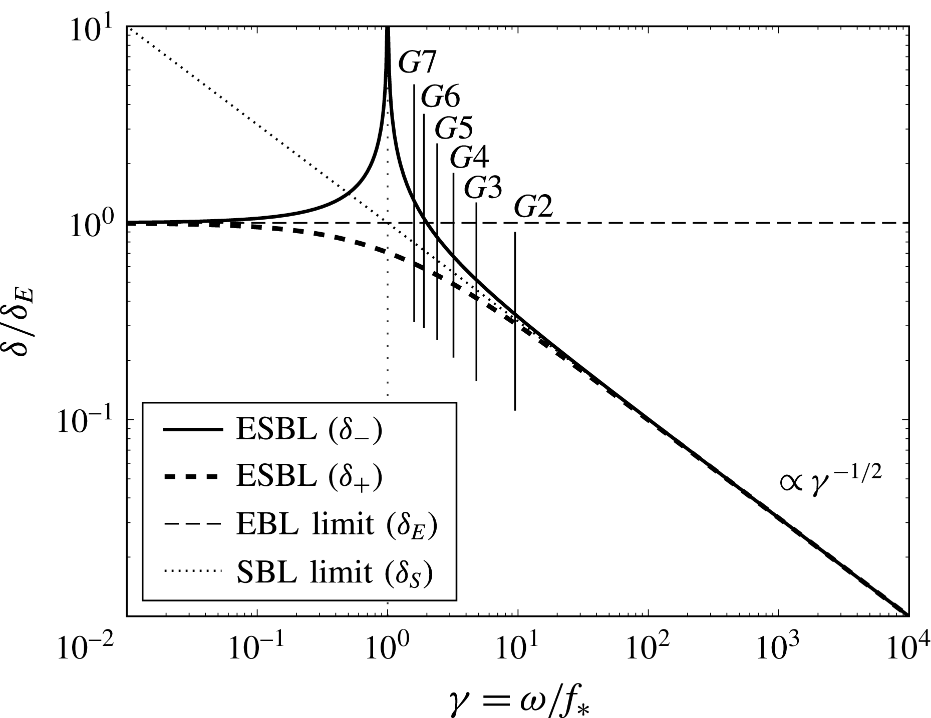
Similarity curve of the ESBL in terms of the theoretical boundary layer thicknesses
 $\unicode[STIX]{x1D6FF}$
as a function of the time scale ratio
 $\unicode[STIX]{x1D6FE}$
. All boundary layer thicknesses have been normalized by the steady EBL thickness
 $\unicode[STIX]{x1D6FF}_{E}$
. The ESBL thickness
 $\unicode[STIX]{x1D6FF}_{-}$
erupts at
 $\unicode[STIX]{x1D6FE}=1$
(solid line), whereas the ESBL thickness
 $\unicode[STIX]{x1D6FF}_{+}$
remains finite (thick dashes). The limiting cases are the steady EBL for
 $\unicode[STIX]{x1D6FE}\ll 1$
(thin dashes) and the SBL for
 $\unicode[STIX]{x1D6FE}\gg 1$
(dotted). Note that the geometries investigated (
 $G2$
–
 $G7$
) are located to the right of the boundary layer eruption.
At intermediate frequencies (
 $\unicode[STIX]{x1D714}$
close to
 $f_{\ast }$
) the ESBL is not so easily described. Figure 2 therefore shows how the ESBL structure changes with
 $\unicode[STIX]{x1D714}$
or
 $f_{\ast }$
when varied over orders of magnitude. More precisely, the normalized boundary layer thicknesses
 $\unicode[STIX]{x1D6FF}_{\pm }/\unicode[STIX]{x1D6FF}_{E}$
is shown as function of the normalized libration frequency
 $\unicode[STIX]{x1D6FE}=\unicode[STIX]{x1D714}/f_{\ast }$
. Due to this scaling, the two graphs shown describe every possible ESBL. The asymptotic behaviour for
 $\unicode[STIX]{x1D6FE}\ll 1$
(EBL) and
 $\unicode[STIX]{x1D6FE}\gg 1$
(SBL) can be observed by means of
 $\unicode[STIX]{x1D6FF}_{\pm }$
converging to a constant value (EBL) or an inclined line (SBL). Only for
 $\unicode[STIX]{x1D714}$
close to
 $f_{\ast }$
(
 $\unicode[STIX]{x1D6FE}\sim O(1)$
) there is a notable difference between
 $\unicode[STIX]{x1D6FF}_{+}$
and
 $\unicode[STIX]{x1D6FF}_{-}$
, and
 $\unicode[STIX]{x1D6FF}_{-}$
diverges at
 $\unicode[STIX]{x1D714}=f_{\ast }$
(
 $\unicode[STIX]{x1D6FE}=1$
). The configurations
 $G2$
–
 $G7$
studied below fulfil
 $\unicode[STIX]{x1D6FE}>1$
and are given by vertical lines. (
 $G1$
is not shown since it has a straight wall with a pure SBL.)
Let us come back to the velocity solution given by (3.8)–(3.10). It is worth noting that the wall-normal velocity
 $w^{\prime }$
does not depend on the frustum radius
 $R$
, but on the local wall-normal vorticity (say
 $f_{\ast }$
) in contrast to the wall-tangential velocities
 $u^{\prime }$
and
 $v^{\prime }$
. The Ekman pumping/suction associated with the induced velocity
 $w^{\prime }$
is maximal for a wall perpendicular to the rotation axis (EBL case
 $|f_{\ast }|=f$
) and reaches zero for an axial wall (SBL case
 $f_{\ast }=0$
). Equations (3.8)–(3.10) show that
 $w^{\prime }$
becomes negligibly small compared to
 $u^{\prime }$
and
 $v^{\prime }$
in case of a very large curvature radius (
 $R\gg 1$
). That is, the kinetic energy density at the wall (
 $u^{\prime 2}\propto R^{2}f^{2}$
) increases with the radius, but the vorticity remains constant (
 $\unicode[STIX]{x1D701}^{\prime }\propto f_{\ast }$
). So, for
 $R\gg 1$
, the solution developed above approaches the planar ESBL studied by Salon & Armenio (Reference Salon and Armenio2011), who considered a pressure-driven (tidally forced) flow on the
 $f$
-plane. This suggests that the boundary layer over the librating frustum is always an ESBL, but it depends on the local wall curvature how strong the Ekman pumping/suction is in comparison to the wall-tangential flow trapped in the boundary layer.
ESBL profiles over the librating frustum at two different libration phases
 $\unicode[STIX]{x1D711}=0$
and
 $\unicode[STIX]{x03C0}/2$
for the geometry
 $G3$
. The analytical solution is compared to the DNS for a wall inclination of
 $\unicode[STIX]{x1D6FC}=6^{\circ }$
towards the axial direction and the libration amplitude
 $\unicode[STIX]{x1D700}=0.2$
(Rossby number
 $Ro=0.2$
) in the stable regime. The origin of the wall-normal coordinate
 $z^{\prime }=0$
corresponds to the point
 $(r,z)\approx (0.905,1.0)$
and all velocity components have been rescaled with the local frustum radius
 $R\approx 0.905$
. The Ekman layer thicknesses
 $\unicode[STIX]{x1D6FF}_{-}$
is given by a dotted vertical line for orientation. The temporal variability is indicated by grey shading between the envelope of the 1-D analytical solutions.

Now that we have the analytical expressions for the laminar velocity profiles we can move on by computing the wall shear stress and the Ekman flux in analogy to (2.8) and (2.9) used for the DNS. This provides further insight into the properties of the ESBL and will proof useful in the analysis of the stable and unstable ESBL addressed later.
The wall shear stress components due to the analytical velocity profiles read
 $$\begin{eqnarray}\displaystyle & \displaystyle \unicode[STIX]{x1D70F}_{\unicode[STIX]{x1D703}}\simeq E\frac{\unicode[STIX]{x2202}u^{\prime }}{\unicode[STIX]{x2202}z^{\prime }}=E\left(-\frac{R}{2}\frac{\unicode[STIX]{x1D6FF}_{-}+\unicode[STIX]{x1D6FF}_{+}}{\unicode[STIX]{x1D6FF}_{-}\unicode[STIX]{x1D6FF}_{+}}\sin (\unicode[STIX]{x1D714}t)-\frac{R}{2}\frac{\unicode[STIX]{x1D6FF}_{-}-\unicode[STIX]{x1D70E}\unicode[STIX]{x1D6FF}_{+}}{\unicode[STIX]{x1D6FF}_{-}\unicode[STIX]{x1D6FF}_{+}}\cos (\unicode[STIX]{x1D714}t)\right), & \displaystyle\end{eqnarray}$$
 $$\begin{eqnarray}\displaystyle & \displaystyle \unicode[STIX]{x1D70F}_{\Vert }\simeq E\frac{\unicode[STIX]{x2202}v^{\prime }}{\unicode[STIX]{x2202}z^{\prime }}=E\left(-\frac{R}{2}\frac{\unicode[STIX]{x1D6FF}_{-}+\unicode[STIX]{x1D70E}\unicode[STIX]{x1D6FF}_{+}}{\unicode[STIX]{x1D6FF}_{-}\unicode[STIX]{x1D6FF}_{+}}\sin (\unicode[STIX]{x1D714}t)+\frac{R}{2}\frac{\unicode[STIX]{x1D6FF}_{-}-\unicode[STIX]{x1D6FF}_{+}}{\unicode[STIX]{x1D6FF}_{-}\unicode[STIX]{x1D6FF}_{+}}\cos (\unicode[STIX]{x1D714}t)\right), & \displaystyle\end{eqnarray}$$
where the boundary layer thicknesses
 $\unicode[STIX]{x1D6FF}_{\pm }$
and the sign
 $\unicode[STIX]{x1D70E}$
have been defined in (3.6).
The Ekman flux is an oscillating mass flux confined to the ESBL. This flux has an azimuthal and a wall-parallel component. The azimuthal component is due to the Stokes property (i.e. momentum diffusion), whereas the wall-parallel component is due to the Ekman property (i.e. Coriolis force). Here, we want to focus on the Ekman property by looking into the wall-parallel component
 $Q$
. Over the frustum,
 $Q$
has radial and axial contributions. Computing
 $Q$
in analogy to (2.9) but here for the analytical velocity profiles yields
 $$\begin{eqnarray}\displaystyle Q=-\frac{\unicode[STIX]{x1D6FF}_{-}+\unicode[STIX]{x1D70E}\unicode[STIX]{x1D6FF}_{+}}{4\unicode[STIX]{x1D70E}}\sin (\unicode[STIX]{x1D714}t)+\frac{\unicode[STIX]{x1D6FF}_{-}-\unicode[STIX]{x1D6FF}_{+}}{4}\cos (\unicode[STIX]{x1D714}t)=A\sin (\unicode[STIX]{x1D714}t+\unicode[STIX]{x1D712}), & & \displaystyle\end{eqnarray}$$
where the amplitude
 $A$
and the phase shift
 $\unicode[STIX]{x1D712}$
are given by
 $$\begin{eqnarray}\displaystyle A=\sqrt{\frac{E}{2}}\sqrt{\frac{f_{\ast }}{f_{\ast }^{2}-\unicode[STIX]{x1D714}^{2}}},\quad \tan \unicode[STIX]{x1D712}=-\frac{\sqrt{f_{\ast }+\unicode[STIX]{x1D714}}-\sqrt{f_{\ast }-\unicode[STIX]{x1D714}}}{\sqrt{f_{\ast }+\unicode[STIX]{x1D714}}+\sqrt{f_{\ast }-\unicode[STIX]{x1D714}}}\quad \text{for }\unicode[STIX]{x1D714}<f_{\ast }, & & \displaystyle\end{eqnarray}$$
 $$\begin{eqnarray}\displaystyle A=\sqrt{\frac{E}{2}}\sqrt{\frac{\unicode[STIX]{x1D714}-\sqrt{\unicode[STIX]{x1D714}^{2}-f_{\ast }^{2}}}{\unicode[STIX]{x1D714}^{2}-f_{\ast }^{2}}},\quad \tan \unicode[STIX]{x1D712}=1\quad \Rightarrow \quad \unicode[STIX]{x1D712}=\unicode[STIX]{x03C0}/4\quad \text{for }\unicode[STIX]{x1D714}>f_{\ast },\quad & & \displaystyle\end{eqnarray}$$
where we assume positive values for
 $f_{\ast }$
and
 $\unicode[STIX]{x1D714}$
. The geometries
 $G2$
–
 $G7$
correspond to the second case where the phase shift is fixed but the amplitude of the induced mass flux depends on the forcing frequency (
 $\unicode[STIX]{x1D714}$
) and the wall inclination (
 $f_{\ast }$
). There are two interesting properties specific to the ESBL: (i) the fixed phase shift (3.16) is a result of the Ekman property by means of a fixed intrinsic time scale
 $f_{\ast }^{-1}$
of the Coriolis force, and (ii) the mass flux amplitude tends to zero for
 $\unicode[STIX]{x1D714}\gg f_{\ast }$
but ‘erupts’ for
 $\unicode[STIX]{x1D714}\rightarrow f_{\ast }$
(Klein et al.
Reference Klein, Seelig, Kurgansky, Ghasemi, Borcia, Will, Schaller, Egbers and Harlander2014). It turns out that small (large) libration frequencies in comparison to the effective Coriolis parameter emphasize the Ekman (Stokes) property of the ESBL. So, in order to have a significant Ekman property in the ESBL, we consider a regime with
 $\unicode[STIX]{x1D714}$
and
 $f_{\ast }$
not too far apart from each other.
3.2 Comparison of the local numerical and analytical ESBL solutions
The DNS requires a finite libration amplitude, which means finite Rossby number and, thus, per se weakly nonlinear conditions. Nevertheless, as long as the flow remains stable, a fair comparison between weakly nonlinear DNS and the linear theory can be performed in the vicinity of the wall. For the case shown in figure 3 a Rossby number of
 $Ro=0.2$
and an Ekman number of
 $E=3\times 10^{-5}$
has been selected such that the flow remained axisymmetric and stable over the frustum. The simulations were conducted as described in § 2. For better comparison with the
 $f$
-plane solution, the velocities
 $(u_{\unicode[STIX]{x1D703}},u_{r},u_{z})$
were transformed to a local reference frame such that
 $(u^{\prime },v^{\prime },w^{\prime })$
denote the local azimuthal, axial (wall parallel in a radial–axial slice), and wall-normal velocity components. Wall-normal velocity profiles (coordinate
 $z^{\prime }$
) have been recorded over a selected location on the frustum.
Figure 3 shows various local wall-normal velocity profiles
 $(u^{\prime },v^{\prime },w^{\prime })$
over the librating frustum comparing the 1-D ESBL solution to the 3-D DNS for the two libration phases
 $\unicode[STIX]{x1D711}=0$
and
 $\unicode[STIX]{x03C0}/2$
. The inclination of the frustum wall is
 $\unicode[STIX]{x1D6FC}=6^{\circ }$
(geometry
 $G3$
), but the flow is representative for all geometries
 $G2$
–
 $G7$
with an inner frustum. Any of the velocity components has been normalized with the local libration velocity
 $Rf/2$
. The temporal variability of the flow is illustrated by a shading of the area between the minimum and maximum values of the 1-D solution.
It is quite remarkable how well the 1-D theory captures the stable 3-D DNS near the wall. The agreement between 1-D theory and DNS is virtually perfect for the wall-tangential components
 $u^{\prime }$
and
 $v^{\prime }$
in figure 3(a,b) up to the five theoretical boundary layer thicknesses (
 $z^{\prime }\leqslant 5\unicode[STIX]{x1D6FF}_{-}$
) shown. By contrast, the wall-normal velocity profile
 $w^{\prime }$
in figure 3(c) deviates notably from the DNS, but especially for
 $z^{\prime }>2\unicode[STIX]{x1D6FF}_{-}$
. This can be explained by curvature and geometry effects. On the one hand, we accounted for curvature only by formulating the boundary conditions on the
 $f$
-plane and then continued with a Cartesian formulation. On the other hand, the 1-D solution does not account for adverse pressure gradients, mean bulk flow (e.g. Sauret et al.
Reference Sauret, Cébron, Le Bars and Le Dizès2012), oscillatory bulk flow due to inertial waves (e.g. Klein et al.
Reference Klein, Seelig, Kurgansky, Ghasemi, Borcia, Will, Schaller, Egbers and Harlander2014) or secondary circulations due to the lids (e.g. Wang Reference Wang1970; Hollerbach & Fournier Reference Hollerbach, Fournier, Bonanno, Rüdiger and Rosner2004). These additional flows are likely to modify the boundary layer structure, in particular the wall-tangential divergence, and are thus likely to have an effect on the wall-normal velocity profile. In any case, the wall-normal velocity is very small compared to the wall-tangential velocity components (
 $u^{\prime }:v^{\prime }:w^{\prime }\approx 1:10^{-1}:10^{-4}$
) and deviations might be less critical.
Note that the larger one (
 $\unicode[STIX]{x1D6FF}_{-}$
) of the two theoretical boundary layer thicknesses
 $\unicode[STIX]{x1D6FF}_{\pm }$
is taken as the overall thickness of the ESBL. This boundary layer thickness is resolved roughly by the distance between the markers shown in figure 3, hence, the mesh size near the wall resolves
 $\unicode[STIX]{x1D6FF}_{-}$
with
 $N_{\unicode[STIX]{x1D6FF}}\approx 4$
grid boxes. This is just good enough to capture the boundary layer structure given the ratio of
 $\unicode[STIX]{x1D6FF}_{-}/\unicode[STIX]{x1D6FF}_{+}\lesssim 1.6$
for the geometries
 $G2$
–
 $G7$
investigated. It is worth to point out that the level of agreement between DNS and the 1-D theory is comparable to the reference results by Lopez & Marques (Reference Lopez and Marques2011) and Salon & Armenio (Reference Salon and Armenio2011), which indicates that the near-wall dynamics is sufficiently resolved in the present DNS and that the 1-D theory is acceptable for the near-wall laminar flow.
In order to study further the effects of nonlinearity, let us come back to the scaling of the governing equations. We can now make use of the laminar boundary layer structure to yield appropriate length scales by means of
 $\unicode[STIX]{x1D6FF}_{\pm }$
(3.6) as well as the well-known boundary layer thicknesses
 $\unicode[STIX]{x1D6FF}_{S}$
of the Stokes layer (e.g. Batchelor Reference Batchelor1967, pp. 353–355) and the thickness
 $\unicode[STIX]{x1D6FF}_{E}$
of the Ekman layer over an inclined wall. Wall libration of the frustum suggests to use the libration frequency to obtain a time scale
 $\unicode[STIX]{x1D714}^{-1}$
and to keep the velocity scale
 $U=\unicode[STIX]{x1D700}\unicode[STIX]{x1D6FA}_{0}r_{1}$
, but to express spatial gradients more carefully with an appropriate length scale. A term-by-term analysis of the momentum balance yields
 $$\begin{eqnarray}\displaystyle \left.\begin{array}{@{}c@{}}\displaystyle \left|\frac{\unicode[STIX]{x2202}\boldsymbol{u}}{\unicode[STIX]{x2202}t}\right|\sim \unicode[STIX]{x1D714},\quad |2\boldsymbol{e}_{z}\times \boldsymbol{u}|\sim f_{\ast },\quad |E\unicode[STIX]{x1D735}\times (\unicode[STIX]{x1D735}\times \boldsymbol{u})|\sim \frac{E}{\unicode[STIX]{x1D6FF}^{2}},\\ \displaystyle |Ro(\boldsymbol{u}\boldsymbol{\cdot }\unicode[STIX]{x1D735})\boldsymbol{u}|\sim \frac{Ro}{\unicode[STIX]{x1D6FF}},\quad |\unicode[STIX]{x1D735}\unicode[STIX]{x1D719}|\sim \frac{Ro}{\unicode[STIX]{x1D6FF}},\end{array}\right\} & & \displaystyle\end{eqnarray}$$
where each term was normalized by
 $\unicode[STIX]{x1D700}^{-1}U^{2}=\unicode[STIX]{x1D700}\unicode[STIX]{x1D6FA}_{0}^{2}r_{1}^{2}$
. Hence,
 $\unicode[STIX]{x1D714}$
and
 $f_{\ast }$
are taken dimensionless relative to the mean rotation rate
 $\unicode[STIX]{x1D6FA}_{0}$
, and the length scale
 $\unicode[STIX]{x1D6FF}$
is dimensionless due to division by the maximum frustum radius
 $r_{1}$
. The balance of forces governs the type of the boundary layer. The viscous term is of the order of
 $E/\unicode[STIX]{x1D6FF}_{S}^{2}=\unicode[STIX]{x1D714}$
for the SBL (
 $\unicode[STIX]{x1D6FF}_{S}=\sqrt{2E/\unicode[STIX]{x1D714}}$
), whereas it is of the order of
 $E/\unicode[STIX]{x1D6FF}_{E}^{2}=f_{\ast }$
for the EBL (
 $\unicode[STIX]{x1D6FF}_{E}=\sqrt{2E/f_{\ast }}$
) and of the order of
 $E/\unicode[STIX]{x1D6FF}_{\pm }^{2}=|\unicode[STIX]{x1D714}\pm f_{\ast }|$
for the ESBL.
For low Rossby numbers and moderate Ekman numbers (not too small boundary layer thickness) equation (3.17) reveals that the local acceleration prescribed by the wall libration and the Coriolis acceleration imposes two time scales. In analogy to Noir et al. (Reference Noir, Calkins, Lasbleis, Cantwell and Aurnou2010), we define the parameter
 $$\begin{eqnarray}\displaystyle \unicode[STIX]{x1D6FE}\equiv \frac{\unicode[STIX]{x1D714}}{f_{\ast }}, & & \displaystyle\end{eqnarray}$$
which expresses the strength of the librational acceleration relative to the (local) Coriolis acceleration in terms of a time scale ratio. Three different flow regimes of the ESBL can be distinguished with the aid of
 $\unicode[STIX]{x1D6FE}$
. These are given by (i)
 $\unicode[STIX]{x1D6FE}\ll 1$
, the rotation-dominated regime with the EBL limit; (ii)
 $\unicode[STIX]{x1D6FE}\sim 1$
, the intermediate or librational–rotational regime with a ‘true’ ESBL; and (iii)
 $\unicode[STIX]{x1D6FE}\gg 1$
, the libration-dominated or viscous regime with the SBL limit. These regimes have been discussed above for the laminar ESBL in terms of
 $\unicode[STIX]{x1D714}$
and
 $f_{\ast }$
instead of
 $\unicode[STIX]{x1D6FE}$
(see pp. 13, below equation (3.11)).
It is illustrative to express the boundary layer thicknesses
 $\unicode[STIX]{x1D6FF}_{\pm }$
in terms of the time scale ratio
 $\unicode[STIX]{x1D6FE}$
to yield
 $$\begin{eqnarray}\displaystyle \unicode[STIX]{x1D6FF}_{\pm }(\unicode[STIX]{x1D6FE})=\frac{\unicode[STIX]{x1D6FF}_{E}}{\sqrt{1\pm \unicode[STIX]{x1D6FE}}}, & & \displaystyle\end{eqnarray}$$
where
 $\unicode[STIX]{x1D6FF}_{E}=\sqrt{2E/f_{\ast }}$
denotes the thickness of the steady EBL over the inclined (frustum) wall. The functional dependency
 $\unicode[STIX]{x1D6FF}_{\pm }(\unicode[STIX]{x1D6FE})$
is shown in figure 2, in which one can distinguish the three flow regimes mentioned. Regime (ii) is located in the central part covering a
 $\unicode[STIX]{x1D6FE}$
-interval of approximately three orders of magnitude centred at
 $\unicode[STIX]{x1D6FE}=1$
. In this regime the two boundary layer thicknesses
 $\unicode[STIX]{x1D6FF}_{\pm }$
are notably different from each other indicating strong competition between the libration and Coriolis time scales. In the limits, regime (i) is approached on the left side for
 $\unicode[STIX]{x1D6FE}<5\times 10^{-2}$
, whereas regime (iii) is approached on the right side for
 $\unicode[STIX]{x1D6FE}>5\times 10^{1}$
. These regimes exhibit a collapse of the two ESBL thicknesses to either the Ekman boundary layer in regime (i) or the Stokes layer in regime (iii). The values of
 $\unicode[STIX]{x1D6FE}$
and
 $\unicode[STIX]{x1D6FF}_{\pm }$
corresponding to geometries
 $G2$
–
 $G7$
are given for orientation and found exclusively to the right of the boundary layer eruption
 $\unicode[STIX]{x1D6FE}=1$
(see table 2 for the exact values). For the geometry
 $G2$
with
 $\unicode[STIX]{x1D6FE}\approx 10$
, still the librational forcing gives the main contribution to the boundary layer dynamics, thus it is categorized as the regime (iii). Increasing
 $\unicode[STIX]{x1D6FC}$
,
 $\unicode[STIX]{x1D6FE}$
gradually decreases and thus the effect of the rotation on the flow dynamics increases in such a way that for the geometry
 $G7$
with
 $\unicode[STIX]{x1D6FE}\approx 1.5$
both rotation and libration give almost the same contribution to the boundary layer dynamics.
The parameter
 $\unicode[STIX]{x1D6FE}$
allows us to estimate fairly easily which of the forces dominates the boundary layer dynamics and, thus, to infer which boundary layer structure is present. This can be relevant for applications, like librating planets or moons, which exhibit all possible wall inclinations thanks to their spherical symmetry, and thus one is left with determining their libration frequency (e.g. Comstock & Bills Reference Comstock and Bills2003). It is worth mentioning that the values of
 $\unicode[STIX]{x1D6FE}$
in table 2 can also be recovered using the maximum ratio of the wall shear stress components as will be discussed in § 3.5 (see table 2,
 $|\unicode[STIX]{x1D70F}_{\unicode[STIX]{x1D703}}|_{+}^{max}/|\unicode[STIX]{x1D70F}_{\Vert }|_{+}^{max}$
).
Until now we have considered only the stable laminar ESBL and used 1-D theory to obtain the axisymmetric near-wall velocity solution over a curved and inclined (conical) wall. In practical applications, however, one is more frequently confronted with (locally) unstable or turbulent flows, which lack specific symmetries. In the following, we will therefore put the focus on nonlinearity, instability and curvature effects by studying the unstable ESBL with DNS for a large libration amplitude (
 $\unicode[STIX]{x1D700}=0.8$
) but moderate Ekman number (
 $E=4\times 10^{-5}$
). We will discuss further the instability mechanism and how it affects the mean flow excited by comparing DNS for the unstable flow regime to those of the stable flow regime.
3.3 Görtler instability of the ESBL
In order to steer the discussion in the direction of the unstable flow conditions, let us begin with a brief review of the laminar flow and the instability mechanism at work in the case of a librating coaxial inner cylinder (geometry
 $G1$
). In this case the induced flow is notably curved, but when the cylinder radius is large compared to the boundary layer thickness, it is well known that an SBL is established over the librating wall and curvature is barely notable for the laminar flow (e.g. Sauret et al.
Reference Sauret, Cébron, Le Bars and Le Dizès2012). The SBL is basically a damped wave, which follows the boundary oscillation and thus yields a strong velocity shear in the vicinity of the librating wall. The absence of the Ekman property is reflected in
 $\unicode[STIX]{x1D6FE}$
tending to infinity, which means that librational forcing and molecular momentum diffusion dominate the flow dynamics exclusively. Non-zero radial and axial velocity components in the DNS are the result of secondary flows that may be due to geometry, nonlinearity and lid effects under stable conditions (e.g. Wang Reference Wang1970; Busse Reference Busse2011) or due to instability (e.g. Noir et al.
Reference Noir, Hemmerlin, Wicht, Baca and Aurnou2009; Sauret et al.
Reference Sauret, Cébron, Le Bars and Le Dizès2012). Focusing on the instability mechanism, it is worth pointing out that the SBL over the librating inner cylinder becomes centrifugally unstable once the libration amplitude exceeds a critical value. This means that curvature effects are vital for the instability. The instability is intermittent and confined to the vicinity of the librating wall. It was reported that structures very much alike Görtler vortices develop. These vortices accelerate the flow locally due to nonlinear advection, which results in a local enhancement of the Coriolis force and leads to a rapid propagation of the Görtler vortices into the fluid bulk (Ghasemi et al.
Reference Ghasemi, Klein, Harlander, Kurgansky, Schaller and Will2016).
The aim of the following paragraphs is to clarify how much of the instability mechanism of the SBL remains in an ESBL. We tackle this question by varying the wall slope of the inner cylinder (frustum).
Contour plots of the instantaneous azimuthal
 $u_{\unicode[STIX]{x1D703}}$
(a–d) and radial velocity component
 $u_{r}$
(e,f) visualizing the Görtler instability of the ESBL for intermittently unstable flows driven by frustum libration with libration amplitude
 $\unicode[STIX]{x1D700}=0.8$
and frequency
 $\unicode[STIX]{x1D714}=1$
using an Ekman number of
 $E=4\times 10^{-5}$
. Panels (a,b,e) on the left correspond to the geometry
 $G2$
, panels (c,d,f) on the right correspond to the geometry
 $G6$
. The contours are shown in axial–radial (a–d) and wall-parallel–azimuthal sections (e,f) of the annular domain. The latter case, the wall-parallel surface is extracted at about
 $2\unicode[STIX]{x1D6FF}_{-}$
. The contours have been recorded at the end of the prograde libration half-period when the instability is fully developed: libration phase
 $\unicode[STIX]{x1D711}=7\unicode[STIX]{x03C0}/8$
(a,c,e,f), and
 $\unicode[STIX]{x1D711}=\unicode[STIX]{x03C0}$
(b,d).

For the selected Ekman number
 $E=\unicode[STIX]{x1D708}/(\unicode[STIX]{x1D6FA}_{0}r_{1}^{2})=4\times 10^{-5}$
all the geometries
 $G1$
–
 $G7$
were found to be unstable for a dimensionless libration amplitude of
 $\unicode[STIX]{x1D700}=0.8$
, and remained stable for
 $\unicode[STIX]{x1D700}=0.2$
. In that respect the ESBL studied here behaves very similar to the SBL investigated by Sauret et al. (Reference Sauret, Cébron, Le Bars and Le Dizès2012) and Ghasemi et al. (Reference Ghasemi, Klein, Harlander, Kurgansky, Schaller and Will2016), i.e. the ESBL becomes centrifugally unstable in the prograde half-phase of a libration cycle. The DNS results shown in figure 4 reveal the generation of Görtler vortices over the librating frustum. A few representative examples of the developed instability are given, whose details and consequences will be discussed further in the following.
Figure 4 shows various contour plots of instantaneous velocity components in different sections of the annular domain. Figure 4(a–d) shows
 $u_{\unicode[STIX]{x1D703}}$
in axial–radial slices for two different configurations
 $G2$
(a,b) and
 $G6$
(c,d), and for two different libration phases
 $\unicode[STIX]{x1D711}=7\unicode[STIX]{x03C0}/8$
and
 $\unicode[STIX]{x03C0}$
at the end of the prograde libration half-period. Figure 4(e,f) shows a wall-parallel–azimuthal section of
 $u_{r}$
for the libration phase
 $\unicode[STIX]{x1D711}=7\unicode[STIX]{x03C0}/8$
at the end of the prograde libration cycle. Geometry
 $G2$
exhibits a small effective Coriolis parameter
 $f_{\ast }$
and represents the transitional regime (iii) where the viscous diffusion is much larger than the Coriolis force (
 $\unicode[STIX]{x1D6FE}\sim O(10)$
). Geometry
 $G6$
exhibits the second largest value of
 $f_{\ast }$
investigated and has
 $\unicode[STIX]{x1D6FE}\sim O(1)$
.
Mushroom-like structures in the axial–radial plane and azimuthally elongated structures along the wall are clearly visible in figures 4(a–d) and 4(e,f), respectively. The later have been obtained by taking a wall-parallel–azimuthal section approximately
 $2\unicode[STIX]{x1D6FF}_{-}$
above the frustum. Streaks of positive
 $u_{r}$
are surrounded by those of negative
 $u_{r}$
which suggests that the propagation of the Görtler vortices out of the ESBL (and into the bulk) is compensated by a local flow entrainment into the ESBL. The close visual correspondence of the elongated vortices in the ESBL and the Görtler vortices observed in an SBL (see Lopez & Marques Reference Lopez and Marques2011; Sauret et al.
Reference Sauret, Cébron, Le Bars and Le Dizès2012; Ghasemi et al.
Reference Ghasemi, Klein, Harlander, Kurgansky, Schaller and Will2016) suggest that the structures in the unstable ESBL are also Görtler vortices. The time sequence of events during the instability development favour this interpretation. Assuming that the Stokes property of the ESBL is the cause of the instability, the analysis of Ghasemi et al. (Reference Ghasemi, Klein, Harlander, Kurgansky, Schaller and Will2016) for a pure SBL can be applied straightforwardly to the ESBL: First, the Görtler vortices are generated by a centrifugal instability mechanism after the frustum started to decelerate. Second, the Görtler vortices propagate radially into the fluid bulk by forming mushroom-like structures that decay as time progresses. The axial–radial sections in figures 4(a,b) and 4(c,d), respectively, reveal the temporal evolution of the Görtler vortices in the ESBL.
An interesting feature of the Görtler vortices in the ESBL is their tilt with respect to the azimuthal coordinate. This tilt is apparent in figure 4(f) and can be quantified by defining a deflection angle
 $\unicode[STIX]{x1D6FD}$
. One could argue that the Coriolis force induces the tilt of the Görtler vortices so that
 $\unicode[STIX]{x1D6FD}$
might not depend on
 $\unicode[STIX]{x1D6FC}$
but rather on the time scale ratio
 $\unicode[STIX]{x1D6FE}=\unicode[STIX]{x1D714}/f_{\ast }$
. The values of
 $\unicode[STIX]{x1D6FC}$
,
 $\unicode[STIX]{x1D6FE}$
and
 $\unicode[STIX]{x1D6FD}$
for the geometries
 $G1$
–
 $G7$
are given in table 2.
Schematic drawing of the laminar boundary layer flow in terms of the boundary layer mass flux
 $\boldsymbol{Q}$
in the unstable phase where Görtler vortices develop (a,b), and the stress angle
 $\unicode[STIX]{x1D6FD}_{\unicode[STIX]{x1D70F}}$
normalized by the vortex deflection angle
 $\unicode[STIX]{x1D6FD}$
as function of the wall inclination angle
 $\unicode[STIX]{x1D6FC}$
(c). Stress angles of the stable and unstable flow have been normalized using
 $\unicode[STIX]{x1D6FD}$
from the
 $\unicode[STIX]{x1D700}=0.8$
case. The streamlines are aligned with the azimuthal coordinate for the inner cylinder (a), but oblique over the frustum (b). The tilt of the streamlines over the frustum tends to increase the effective curvature radius of the local flow (
 $r^{\prime \prime }>r^{\prime }$
for locally comparable wall radii).
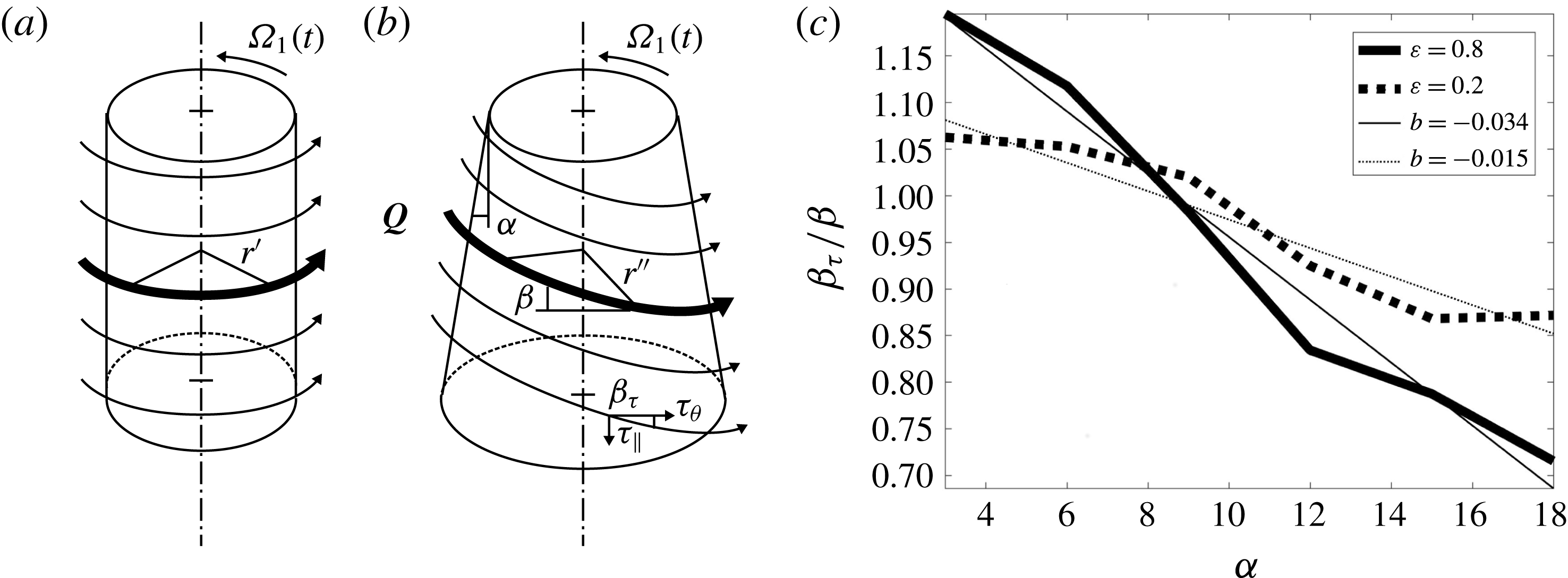
The tilt of the Görtler vortices can be related to the direction of the flow within the boundary layer, that is, the direction of the wall shear stress that will be discussed in detail in § 3.5. Figure 5(a,b) shows a sketch of the flow along the inner cylinder (a) and the inner frustum (b) during the unstable phase of the libration cycle. The flow is not just azimuthal in the case of the frustum like for the pure Stokes boundary layer and neither just down slope like for the pure Ekman flux. The sum of both effects leads to a spiral-shaped downward flow and the Görtler vortices will be mainly oriented parallel to this flow. This can be analysed quantitatively by comparing the deflection angle
 $\unicode[STIX]{x1D6FD}$
to the components of the wall shear stress components
 $\tan \unicode[STIX]{x1D6FD}_{\unicode[STIX]{x1D70F}}=|\unicode[STIX]{x1D70F}_{\Vert }|_{+}^{max}/|\unicode[STIX]{x1D70F}_{\unicode[STIX]{x1D703}}|_{+}^{max}$
(see table 2). Figure 5(c) shows the normalized stress angle
 $\unicode[STIX]{x1D6FD}_{\unicode[STIX]{x1D70F}}/\unicode[STIX]{x1D6FD}$
as a function of the wall slope
 $\unicode[STIX]{x1D6FC}$
. This normalization is arbitrary for
 $\unicode[STIX]{x1D700}=0.2$
since there are no Görtler vortices for this case. Under these stable conditions,
 $\unicode[STIX]{x1D6FD}_{\unicode[STIX]{x1D70F}}/\unicode[STIX]{x1D6FD}$
can be interpreted as the tilt angle that could be expected if the flow would be unstable for
 $\unicode[STIX]{x1D700}=0.2$
. As can be seen in figure 5(c), for both stable and unstable conditions, with increasing cone angle
 $\unicode[STIX]{x1D6FC}$
the stress angle
 $\unicode[STIX]{x1D6FD}_{\unicode[STIX]{x1D70F}}$
becomes slightly smaller than the Görtler vortex deflection angle
 $\unicode[STIX]{x1D6FD}$
but the dependency is rather weak. Linear regression
 $\unicode[STIX]{x1D6FD}_{\unicode[STIX]{x1D70F}}/\unicode[STIX]{x1D6FD}=b\unicode[STIX]{x1D6FC}+c$
yields a slope of
 $b=-0.034$
for
 $\unicode[STIX]{x1D700}=0.8$
and
 $b=-0.015$
for
 $\unicode[STIX]{x1D700}=0.2$
, respectively. This has an interesting consequence. The effective curvature radius
 $r^{\prime \prime }$
increases with
 $\unicode[STIX]{x1D6FC}$
as sketched in figure 5(b) so that a critical value of
 $\unicode[STIX]{x1D6FC}$
can be expected above which the Görtler instability will vanish. We will see later that the Görtler instability is the main driver for a bulk mean flow, which means we can expect that for large cone angle
 $\unicode[STIX]{x1D6FC}$
this mean flow will be significantly reduced.
Finally we give the power scaling of the deflection angle
 $\unicode[STIX]{x1D6FD}$
with respect to
 $\unicode[STIX]{x1D6FC}$
and
 $\unicode[STIX]{x1D6FE}=\unicode[STIX]{x1D714}/(2\unicode[STIX]{x1D6FA}_{0}\sin \unicode[STIX]{x1D6FC})$
. For the values listed in table 2 we find
 $$\begin{eqnarray}\displaystyle \unicode[STIX]{x1D6FD}(\unicode[STIX]{x1D6FC})\approx 1.48\unicode[STIX]{x1D6FC}^{0.89}\quad \text{and}\quad \unicode[STIX]{x1D6FD}(\unicode[STIX]{x1D6FE})\approx 29.4\unicode[STIX]{x1D6FE}^{-0.89}, & & \displaystyle\end{eqnarray}$$
which yields a close-to-linear dependency of the deflection angle on any of the librating wall’s inclination parameters. This is because the values of
 $\unicode[STIX]{x1D6FC}$
are small (
 $\unicode[STIX]{x1D6FC}\leqslant 18^{\circ }$
), so that a dependency on
 $\sin \unicode[STIX]{x1D6FC}$
is not notable because of the uncertainty in
 $\unicode[STIX]{x1D6FD}$
. The almost linear dependencies confirm that the cause of the Görtler vortex deflection is the Ekman flux
 $Q$
along the inner cone, which is given by (3.14) and (3.16) for the stable boundary layer here.
In order to clarify what determines the deflection of the Görtler instability, the near-wall flow structure has to be addressed more carefully. The laminar ESBL discussed in the previous section provides the environment in which the instability develops. We will therefore discuss the relevance of the Ekman flux and the wall shear stress in the following two sections.
3.4 Ekman flux of the ESBL under stable and unstable flow conditions
The axial displacement of the Görtler vortices can be related to the oscillating Ekman flux by considering the time scales of the instability and the forcing. The Görtler vortices develop only during a fraction of the prograde libration cycle, that is, between libration phase
 $\unicode[STIX]{x1D711}=\unicode[STIX]{x03C0}/2$
and
 $\unicode[STIX]{x03C0}$
. In the remaining
 $3/4$
of a libration period the Görtler vortices merely decay while propagating towards the fluid bulk. This suggests that the Ekman flux properties are only important in the fraction of the libration period during which the Görtler vortices develop.
To assess this further, we assume that the Ekman flux
 $Q$
is dominated by linear dynamics with a laminar near-wall flow, which is described by the analytical solution given by (3.14) and (3.16). For the geometries studied here we have to select the case with constant phase shift (
 $\unicode[STIX]{x1D712}=\unicode[STIX]{x03C0}/4$
). The amplitude is positive (
 $A>0$
) so that the Ekman flux becomes negative,
 $$\begin{eqnarray}\displaystyle Q=A\sin (\unicode[STIX]{x1D711}+\unicode[STIX]{x1D712})<0\quad \text{for }3\unicode[STIX]{x03C0}/4<\unicode[STIX]{x1D711}<7\unicode[STIX]{x03C0}/4. & & \displaystyle\end{eqnarray}$$
Remember that the local axes used for the analytical computation is oriented such that
 $Q>0$
corresponds to axially upward flow. Consequently, the Görtler vortices start to develop at
 $\unicode[STIX]{x1D711}=\unicode[STIX]{x03C0}/2$
in the ESBL with some upward directed Ekman flux, which decreases gradually while the Görtler vortices intensify. (This is supported also by the DNS results in figure 6 to be discussed shortly.) From there on, the Görtler vortices are immersed in a downward directed Ekman flux until they have decayed or left the Ekman flux influence region of the ESBL.
The evolution of the wall-parallel Ekman flux
 $Q$
over one libration period for statistically stationary flow conditions is shown in figure 6 for all the geometries investigated. Figure 6(a) shows the DNS results for the stable ESBL excited by wall libration with the dimensionless amplitude
 $\unicode[STIX]{x1D700}=0.2$
, whereas figure 6(b) shows those for the intermittently unstable ESBL excited with
 $\unicode[STIX]{x1D700}=0.8$
. The dimensionless libration frequency
 $\unicode[STIX]{x1D714}=1$
and the Ekman number
 $E=4\times 10^{-5}$
were kept constant.
The simulated Ekman fluxes
 $Q$
in the stable ESBLs shown in figure 6(a) are sinusoidal in time as expected from the analytical analysis. All time series pass through the same zero crossings at
 $\unicode[STIX]{x1D711}\approx 5\unicode[STIX]{x03C0}/8$
and
 $13\unicode[STIX]{x03C0}/8$
and the local extrema can be found half-way in between. This is interesting, since the phase shift is larger in comparison to the analytical solution given by (3.14) and (3.16). The origin of the remaining phase shift is not clear yet but potentially related to an interaction of the ESBL with the excited bulk flow. (We will discuss the mean bulk flow further in § 3.6.) For the rest, the Ekman flux of the stable ESBL agrees with the analytical solution, in particular with respect to the increase in amplitude together with cone angle due to an increase of the effective Coriolis force.
Evolution of the spatially averaged wall-parallel mass flux
 $Q$
(Ekman flux) scaled with the dimensionless libration amplitude
 $\unicode[STIX]{x1D700}$
for statistically stationary flow conditions.
 $Q$
is a property of the ESBL driven up and down the librating frustum during one libration cycle. DNS results are shown for stable flow conditions excited with
 $\unicode[STIX]{x1D700}=0.2$
(a) and intermittently unstable flow conditions excited with
 $\unicode[STIX]{x1D700}=0.8$
(b). Time series are shown for all geometries
 $G1$
–
 $G7$
and exhibit an increase of
 $Q/\unicode[STIX]{x1D700}$
with the cone angle
 $\unicode[STIX]{x1D6FC}$
of the frustum. The grey region indicates the time interval of the development of the Görtler instability.

The simulated Ekman fluxes
 $Q$
in the intermittently unstable ESBL shown in figure 6(b) are neither sinusoidal nor symmetric even though the sinusoidal forcing is still dominating the time series. For this unstable flow regime, the negative part of the time series of
 $Q$
between
 $\unicode[STIX]{x1D711}=5\unicode[STIX]{x03C0}/8$
and
 $13\unicode[STIX]{x03C0}/8$
is notably modified, which can be attributed to the development of Görtler vortices for libration phases
 $\unicode[STIX]{x1D711}\geqslant \unicode[STIX]{x03C0}/2$
. However, once the Görtler vortices have decayed the laminar solution starts to dominate again for
 $\unicode[STIX]{x1D711}\gtrsim 7\unicode[STIX]{x03C0}/4$
. Consequently, the positive part of the time series of
 $Q$
is comparable to the stable regime (compare with figure 6
a).
The Ekman flux is affected more by the Görtler vortices when the cone angle
 $\unicode[STIX]{x1D6FC}$
and the effective Coriolis parameter
 $f_{\ast }$
are small and the time scale ratio
 $\unicode[STIX]{x1D6FE}$
is large. In the case of geometry
 $G2$
in figure 6(a,b), for example, the minimum value of
 $Q$
reached at
 $\unicode[STIX]{x1D711}\approx 9\unicode[STIX]{x03C0}/8$
in the stable regime is about eight times larger in magnitude than the corresponding value of
 $Q$
in the intermittently unstable flow regime. With increasing
 $\unicode[STIX]{x1D6FC}$
or
 $f_{\ast }$
(decreasing
 $\unicode[STIX]{x1D6FE}$
) the negative values of
 $Q$
in the unstable flow regime are much closer to the values obtained in the stable flow regime. For the geometry
 $G7$
in figure 6(a,b), for example, the minimum value of
 $Q$
reached at
 $\unicode[STIX]{x1D711}\approx 9\unicode[STIX]{x03C0}/8$
in the stable flow regime is only approximately
 $1.16$
times larger in magnitude than the corresponding value in the unstable flow regime. Altogether, the Coriolis force (as property of the ESBL) appears to have a stabilizing effect on the boundary layer flow. We therefore conjecture that there is a critical cone angle
 $\unicode[STIX]{x1D6FC}_{c}$
(wall slope) above (below) which the Görtler instability ceases to exist for given values of the similarity parameters
 $\unicode[STIX]{x1D6FE}$
and
 $E$
of the laminar ESBL. The proof of this conjecture is beyond the scope of the present study but would be worth addressing elsewhere.
With close with noting that the development of the Görtler vortices causes near-wall mixing of angular momentum. The negative part of the time series of
 $Q$
is notably flattened (figure 6
b), which indicates that the structure of the ESBL is partly destroyed, but only temporarily. Therefore, not only the Görtler vortices are affected by the Ekman flux, but also the Ekman flux is modified by the Görtler vortices.
3.5 Wall shear stress components under stable and unstable flow conditions
For the geometry
 $G2$
with cone angle
 $\unicode[STIX]{x1D6FC}=3^{\circ }$
and effective dimensionless Coriolis parameter
 $f_{\ast }\approx 0.1$
it follows that the time scale ratio is
 $\unicode[STIX]{x1D6FE}\approx 10$
. Thus, according to the classification above, librational forcing dominates the boundary layer flow and the boundary layer is almost a Stokes layer. With
 $\unicode[STIX]{x1D6FC}$
increasing from
 $G2$
to
 $G7$
,
 $\unicode[STIX]{x1D6FE}$
decreases gradually to about
 $1.6$
so that the Coriolis force influences more and more the boundary layer dynamics. This change in quality is exhibited not only by the boundary layer thickness (see figure 2) but also by the wall shear stress, which is very sensitive to the flow structure above the wall. The wall shear stress components
 $\unicode[STIX]{x1D70F}_{\unicode[STIX]{x1D703}}$
and
 $\unicode[STIX]{x1D70F}_{\Vert }$
(as defined by (2.8)) contain information about the ESBL and can therefore be used to characterize the boundary layer in addition to or as an alternative to the time scale ratio
 $\unicode[STIX]{x1D6FE}$
. The stable ESBL excited with the dimensionless libration amplitude
 $\unicode[STIX]{x1D700}=0.2$
is accurately described by the analytical solution (see (3.8)–(3.10) figure 3) so that we focus on the unstable ESBL in the following paragraphs.
Evolution of the azimuthal wall shear stress component
 $\unicode[STIX]{x1D70F}_{\unicode[STIX]{x1D703}}$
(a) and the almost axial along-wall component
 $\unicode[STIX]{x1D70F}_{\Vert }$
(b) during a libration cycle in the case of statistically stationary flow conditions in the intermittently unstable flow regime (dimensionless libration amplitude
 $\unicode[STIX]{x1D700}=0.8$
). Time series are shown for various geometries (
 $G1$
–
 $G7$
) with different wall inclinations (cone angles
 $\unicode[STIX]{x1D6FC}=0^{\circ }$
–
 $16^{\circ }$
). The Ekman number and dimensionless libration frequency were fixed at
 $E=4\times 10^{-5}$
and
 $\unicode[STIX]{x1D714}=1$
, respectively. The grey region indicates the time interval of the developing Görtler instability.
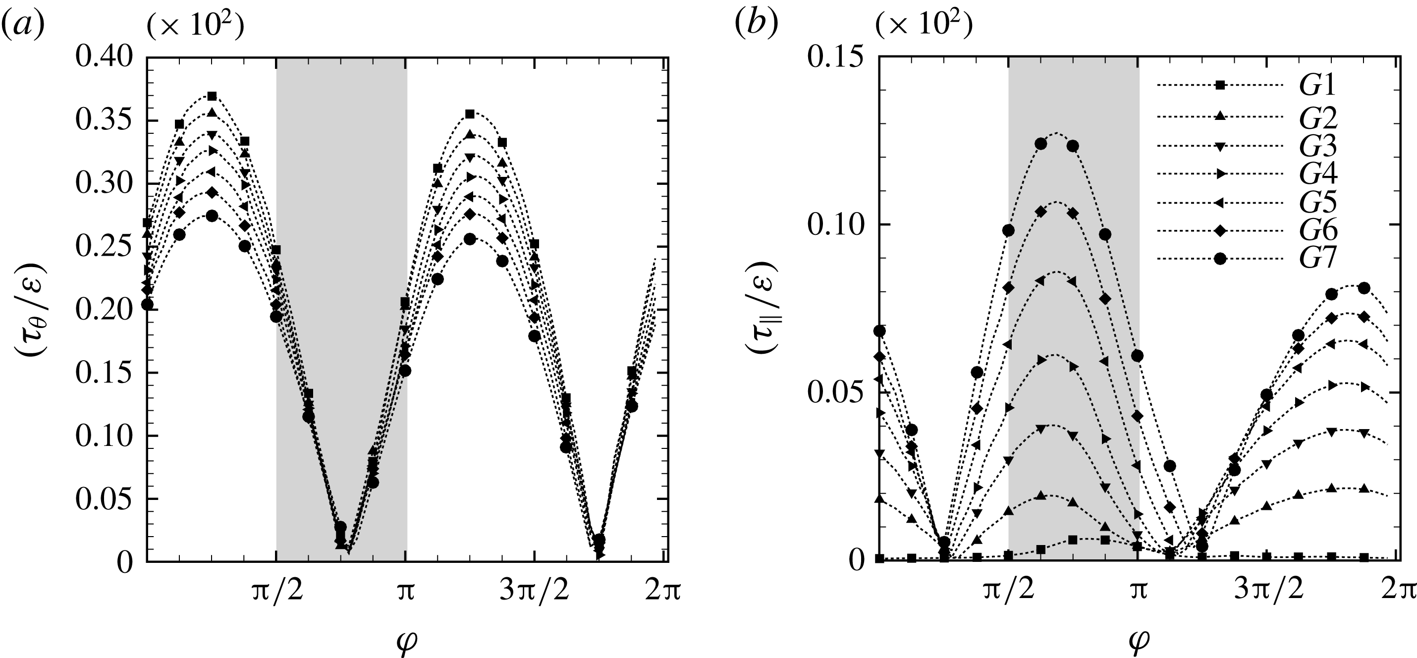
Figure 7 shows various simulated time series of the scaled wall shear stress components
 $\unicode[STIX]{x1D70F}_{\unicode[STIX]{x1D703}}/\unicode[STIX]{x1D700}$
and
 $\unicode[STIX]{x1D70F}_{\Vert }/\unicode[STIX]{x1D700}$
covering a complete libration period for the flow in the statistically stationary state under intermittently unstable flow conditions (
 $\unicode[STIX]{x1D700}=0.8$
). Each profile corresponds to one of the geometries
 $G1$
–
 $G7$
. The wall shear stress is scaled with
 $\unicode[STIX]{x1D700}$
in analogy to the 1-D boundary layer solution given by (3.12) and (3.13). For all geometries investigated, the boundary layer over the inner librating wall becomes unstable in the prograde half-phase of libration just after the wall libration has passed its maximum amplitude at
 $\unicode[STIX]{x1D711}=\unicode[STIX]{x03C0}/2$
, which is precisely the onset of the wall deceleration.
The azimuthal component of the wall shear stress
 $\unicode[STIX]{x1D70F}_{\unicode[STIX]{x1D703}}$
is shown in figure 7(a) and reaches its maximum value at
 $\unicode[STIX]{x1D711}\approx \unicode[STIX]{x03C0}/4$
during the prograde half-phase of libration. The amplitude decreases with increasing cone angle
 $\unicode[STIX]{x1D6FC}$
from
 $G1$
to
 $G7$
due to stronger Coriolis force effects. The time series of
 $\unicode[STIX]{x1D70F}_{\unicode[STIX]{x1D703}}$
are almost symmetric in the prograde and retrograde libration half-phases. This indicates that the Görtler instability has only a weak effect along the azimuth, which is therefore the direction with merely linear dynamics.
The axial component of the wall shear stress
 $\unicode[STIX]{x1D70F}_{\Vert }$
is shown in figure 7(b) and reaches its maximum value at
 $\unicode[STIX]{x1D711}\approx 3\unicode[STIX]{x03C0}/4$
, which is also in the prograde half-phase of libration but phase shifted by
 $\unicode[STIX]{x0394}\unicode[STIX]{x1D719}=\unicode[STIX]{x03C0}/2$
with respect to
 $\unicode[STIX]{x1D70F}_{\unicode[STIX]{x1D703}}$
. The maximum value increases with the cone angle
 $\unicode[STIX]{x1D6FC}$
or the wall-parallel component of the Coriolis force, respectively. This suggests that the straight cylinder case
 $G1$
has
 $\unicode[STIX]{x1D70F}_{\Vert }\neq 0$
only because the developing Görtler instability (compare with Sauret et al.
Reference Sauret, Cébron, Le Bars and Le Dizès2012; Ghasemi et al.
Reference Ghasemi, Klein, Harlander, Kurgansky, Schaller and Will2016) since the SBL lacks a boundary layer mass flux in the axial direction. The time series of
 $\unicode[STIX]{x1D70F}_{\Vert }$
are not symmetric with respect to the prograde and retrograde libration half-periods in contrast to
 $\unicode[STIX]{x1D70F}_{\unicode[STIX]{x1D703}}$
. This indicates a strong effect of the Görtler instability (i.e. nonlinear dynamics) in the along-wall direction. In fact, the Görtler vortices yield the largest gradients (shear) approximately in axial direction (see figure 4
e,f).
It is worth to note that the magnitudes of
 $\unicode[STIX]{x1D70F}_{\unicode[STIX]{x1D703}}$
and
 $\unicode[STIX]{x1D70F}_{\Vert }$
are comparable in the DNS results. Moreover, the phase shifts of
 $\unicode[STIX]{x03C0}/4$
and
 $3\unicode[STIX]{x03C0}/4$
to the libration exhibited by
 $\unicode[STIX]{x1D70F}_{\unicode[STIX]{x1D703}}$
and
 $\unicode[STIX]{x1D70F}_{\Vert }$
, respectively, are present in the DNS results and the 1-D laminar boundary layer solution, ((3.12) and (3.13), case with
 $\unicode[STIX]{x1D714}>f_{\ast }$
and
 $\unicode[STIX]{x1D70E}=-1$
). This suggests that there is a trace of both the linear and nonlinear dynamics. The azimuthal flow is dominated by the viscous linear dynamics due to the forcing, whereas the axially directed flow is dominated by the nonlinear dynamics of the Görtler vortices.
Furthermore, note that the evolution of the wall shear stress components for stable flow conditions is perfectly sinusoidal and qualitatively similar to the Ekman flux shown in figure 6(a). The time series are therefore not shown here, but the corresponding values of the wall shear stress components are given in table 2. It is quite interesting that the ratio of the wall shear stress components
 $|\unicode[STIX]{x1D70F}_{\unicode[STIX]{x1D703}}|_{+}^{max}/|\unicode[STIX]{x1D70F}_{\Vert }|_{+}^{max}$
during prograde libration is comparable for the stable and intermittently unstable ESBL (see table 2). This ratio apparently scales with
 $\unicode[STIX]{x1D6FE}$
so that its maximum value may be used for the flow regime identification of the ESBL as an alternative to
 $\unicode[STIX]{x1D6FE}$
. The ratio
 $|\unicode[STIX]{x1D70F}_{\Vert }|_{+}^{max}/|\unicode[STIX]{x1D70F}_{\Vert }|_{-}^{max}$
reflects the asymmetry of the Ekman fluxes observed in the prograde and retrograde libration half-periods. For the stable ESBL, this ratio shows an asymmetry of approximately
 $15\,\%$
. For the intermittently unstable ESBL, the asymmetry increases with increasing cone angle
 $\unicode[STIX]{x1D6FC}$
so that it is approximately
 $65\,\%$
for the geometry
 $G7$
.
The maximum axial wall shear stress
 $|\unicode[STIX]{x1D70F}_{\Vert }|_{+}^{max}$
is notably different for the stable and unstable flow conditions (see table 2). It exhibits an approximately linear dependency on the effective Coriolis parameter
 $f_{\ast }$
corresponding to an approximately inverse proportionality to
 $\unicode[STIX]{x1D6FE}$
(provided the libration frequency is constant), that is,
 $$\begin{eqnarray}\displaystyle |\unicode[STIX]{x1D70F}_{\Vert }|_{+}^{max}\approx \left\{\begin{array}{@{}l@{}}0.0028\unicode[STIX]{x1D6FE}^{-0.90}\quad \text{for }\unicode[STIX]{x1D700}=0.2,\\ 0.0034\unicode[STIX]{x1D6FE}^{-1.02}\quad \text{for }\unicode[STIX]{x1D700}=0.8.\end{array}\right. & & \displaystyle\end{eqnarray}$$
A similar analysis for the maximum azimuthal wall shear stress
 $|\unicode[STIX]{x1D70F}_{\unicode[STIX]{x1D703}}|_{+}^{max}$
(see table 2) reveals only a weak dependency on
 $\unicode[STIX]{x1D6FE}$
, namely
 $|\unicode[STIX]{x1D70F}_{\unicode[STIX]{x1D703}}|_{+}^{max}\approx 0.27\unicode[STIX]{x1D6FE}^{0.13}$
, for both the intermittently unstable (
 $\unicode[STIX]{x1D700}=0.8$
) and stable (
 $\unicode[STIX]{x1D700}=0.2$
) ESBLs. From geometry
 $G2$
to
 $G7$
,
 $|\unicode[STIX]{x1D70F}_{\unicode[STIX]{x1D703}}|_{+}^{max}$
changes by almost
 $20\,\%$
. But at the same time also the mean frustum radius
 $r_{m}=(r_{1}+r_{3})/2$
changes from
 $r_{m}=1$
(
 $G1$
) to
 $r_{m}=0.8$
(
 $G7$
) which is precisely a
 $20\,\%$
difference. This suggests that the variation of
 $|\unicode[STIX]{x1D70F}_{\unicode[STIX]{x1D703}}|_{+}^{max}$
is merely due to geometry and a result of the change of the wall velocity due to smaller mean frustum radius at larger cone angle
 $\unicode[STIX]{x1D6FC}$
.
So, what will be the net effect of the intermittently unstable ESBL flow? We address this question in the following by investigating the generation of azimuthal mean flows by distinguishing the stable and unstable ESBL.
3.6 Mean flow generation due to Görtler vortices in the unstable ESBL
In this section we focus on the generation mechanism of the mean flow in the case of an intermittently unstable ESBL (excited with the dimensionless libration amplitude
 $\unicode[STIX]{x1D700}=0.8$
). We do not discuss in detail the mean flow generation mechanism in the case of a stable ESBL (
 $\unicode[STIX]{x1D700}=0.2$
), but we will describe important properties of this mean flow for comparison.
Figure 8 shows radial profiles of the scaled time-mean azimuthal velocity
 $\langle \widetilde{u}_{\unicode[STIX]{x1D703}}\rangle _{\unicode[STIX]{x1D703}}/\unicode[STIX]{x1D700}^{2}$
(see § 2.5 for the definition of the mean) for the geometry
 $G2$
in the libration-dominated regime (iii) and
 $G6$
in the intermediate rotation-libration regime (ii), respectively. The mean flow is either due to a stable (figure 8
a,b) or unstable (figure 8
c,d) boundary layer flow. The corresponding radial profiles of the azimuthal mean velocity extracted at the axial position
 $z=1.2$
are shown in figure 8(e,f). In the following, we describe first the mean flow due to a stable ESBL and afterwards that due to the unstable ESBL.
Azimuthal mean flow
 $\langle \widetilde{u}_{\unicode[STIX]{x1D703}}\rangle _{\unicode[STIX]{x1D703}}/\unicode[STIX]{x1D700}^{2}$
for the stable (a,b) and intermittently unstable (c,d) ESBLs for the geometries
 $G2$
(a,c) and
 $G6$
(b,d). Radial profile of
 $\langle \widetilde{u}_{\unicode[STIX]{x1D703}}\rangle _{z\unicode[STIX]{x1D703}}/\unicode[STIX]{x1D700}^{2}$
at axial height
 $z=1.2$
for all the geometries from
 $G1$
to
 $G7$
for the stable (e) and intermittently unstable (f) ESBLs.

In the case of the stable ESBL (figure 8
a,b), both geometries
 $G2$
and
 $G6$
exhibit a prograde jet-like structure in the azimuthal mean velocity field. This jet originates from the bottom corner, extends to the top lid and aligns then with the rotation axis. For the geometry
 $G2$
, the cone angle is small (
 $\unicode[STIX]{x1D6FC}=3^{\circ }$
) so that the prograde jet remains attached to the frustum. This is different for the geometry
 $G6$
, where the wall is more oblique (
 $\unicode[STIX]{x1D6FC}=15^{\circ }$
) and the prograde jet has notably detached from the frustum at heights
 $z\geqslant 0.4$
. In addition, one can also see a retrograde mean flow between the frustum and the prograde jet. The radial profiles shown in figure 8(e) reveal that the position of the maximum of the prograde jet is quite stable and located at radial position
 $r=1.02$
for the geometries
 $G2$
–
 $G7$
investigated. Geometry
 $G1$
is somewhat different as it exhibits a SBL over the inner wall and only a weak prograde jet close to the inner cylinder (see also Ghasemi et al.
Reference Ghasemi, Klein, Harlander, Kurgansky, Schaller and Will2016, figure 3).
The prograde jet shown in figure 8(e) exhibits a dependency on the wall inclination in addition to the compensated
 $\unicode[STIX]{x1D700}^{2}$
-dependency. The magnitude of the jet increases with the cone angle
 $\unicode[STIX]{x1D6FC}$
or the local Coriolis parameter
 $f_{\ast }$
, respectively. The maximum jet velocity
 $\langle \widetilde{u}_{\unicode[STIX]{x1D703}}\rangle _{\unicode[STIX]{x1D703}}^{max}/\unicode[STIX]{x1D700}^{2}$
is located at
 $z=1.2$
and
 $r=1.02$
and exhibits an almost linear dependency on
 $f_{\ast }$
. A least-squares fit of the data gives
 $$\begin{eqnarray}\displaystyle \langle \widetilde{u}_{\unicode[STIX]{x1D703}}\rangle _{\unicode[STIX]{x1D703}}^{max}/\unicode[STIX]{x1D700}^{2}=0.23f_{\ast }^{1.14}. & & \displaystyle\end{eqnarray}$$
It is interesting that the structure of the prograde jet shown in figure 8(e) is reminiscent of the Stewartson layer in a librating spherical shell geometry, in which it is caused by the boundary layer ‘eruption’ at the equator (see e.g. Sauret & Le Dizès Reference Sauret and Le Dizès2013). For the present geometry, however, the origin of this ‘Stewartson layer’ is not yet fully clear. It seems that the divergence of the wall-tangential Ekman flux near the corners adjacent to librating parts of the wall (here in particular the bottom inner corner) is crucial. This hypothesis is supported by the localized boundary layer eruption of the corner flow suggested by Klein et al. (Reference Klein, Seelig, Kurgansky, Ghasemi, Borcia, Will, Schaller, Egbers and Harlander2014).
It is also worth noting that the retrograde mean flow is absent for the geometries
 $G1$
and
 $G2$
(see figure 8
e). The generation mechanism for this retrograde flow is completely unclear at present. We conjecture that it is due to the recurrence of low frequency inertial waves to the frustum. These waves propagate mainly in axial direction so that they can get focused towards the upper inner corner provided their frequency is low enough or the cone angle of the frustum large enough (for details see Borcia & Harlander Reference Borcia and Harlander2012; Klein et al.
Reference Klein, Seelig, Kurgansky, Ghasemi, Borcia, Will, Schaller, Egbers and Harlander2014). This scenario yields strong localization of wave energy and momentum in the vicinity of the upper inner corner so that the ‘trapped’ waves can interact nonlinearly with each other and/or the ESBL. The retrograde mean flow follows from mixing of background angular momentum (e.g. Maas Reference Maas2001).
In the case of the intermittently unstable ESBL, the prograde azimuthal mean flow tends to cover a larger radial fraction of the domain (figure 8
c,d) in comparison to the stable ESBL (figure 8
a,b). This is even better visible in figure 8(f), where the radial profiles of the compensated azimuthal mean velocity
 $\langle \widetilde{u}_{\unicode[STIX]{x1D703}}\rangle _{\unicode[STIX]{x1D703}}/\unicode[STIX]{x1D700}^{2}$
are shown. One can see that the prograde mean flow is typically composed of two peaks for the geometries
 $G2$
to
 $G5$
which suggests presence of two different generation mechanisms. The first local maximum is located closer to the librating frustum and the second further away towards the bulk. The first is larger than the second for the geometry
 $G2$
, while it becomes smaller than the second for
 $G3$
–
 $G5$
, and disappears for the geometries
 $G6$
and
 $G7$
. The first maximum decreases with increasing cone angle
 $\unicode[STIX]{x1D6FC}$
or local Coriolis parameter
 $f_{\ast }$
, respectively.
It is worth noting that the mean flow magnitude in the case of an unstable ESBL approaches
 $\langle \widetilde{u}_{\unicode[STIX]{x1D703}}\rangle _{\unicode[STIX]{x1D703}}^{max}/\unicode[STIX]{x1D700}^{2}\approx 0.09$
whereas it keeps increasing in the case of the stable ESBL (see lines for
 $G2$
–
 $G7$
in figure 8
e,f). The results in figure 8(f) reveal that the approximately linear dependency
 $\langle \widetilde{u}_{\unicode[STIX]{x1D703}}\rangle _{\unicode[STIX]{x1D703}}^{max}/\unicode[STIX]{x1D700}^{2}\propto f_{\ast }$
according to (3.23) is not valid for the unstable ESBL.
Geometry
 $G1$
yields an interesting limit by exhibiting only a single-peaked jet (first maximum). This suggests dominance of one generation mechanism. The maximum value
 $\langle \widetilde{u}_{\unicode[STIX]{x1D703}}\rangle _{\unicode[STIX]{x1D703}}^{max}/\unicode[STIX]{x1D700}^{2}$
is located in the vicinity of the frustum wall and exhibits a jump of more than an order of magnitude when the ESBL changes from stable to unstable flow conditions. It is the result of the generation of Görtler vortices in the unstable SBL (Ghasemi et al.
Reference Ghasemi, Klein, Harlander, Kurgansky, Schaller and Will2016) and this behaviour is still visible in the geometry
 $G2$
. So, what happens for the geometries
 $G3$
–
 $G7$
?
For larger wall inclination angles
 $\unicode[STIX]{x1D6FC}$
(measured relative to the axis), not only does the ESBL becomes thicker (see table 1) but also the deflection angle
 $\unicode[STIX]{x1D6FD}$
of the Görtler vortices increases (see figure 4 and table 2). This suggests that, with increasing
 $\unicode[STIX]{x1D6FC}$
or
 $f_{\ast }$
, the Görtler vortices travel further within the ESBL and decay partly there. This leaves less momentum and kinetic energy for the mean flow driven in the bulk (Ghasemi et al.
Reference Ghasemi, Klein, Harlander, Kurgansky, Schaller and Will2016).
The intensity of the Görtler vortices is not only reduced due to inertial (upscale energy transfer to the mean flow) and viscous losses, but also due to the cylindrical geometry. As discussed at the end of the § 3.5, the mean radius of the frustum decreases with increasing
 $\unicode[STIX]{x1D6FC}$
and so does the resultant prograde mean flow due to weaker background angular momentum near the librating frustum wall. Consequently, for a fixed axial position
 $z$
well above the bottom lid, the contribution of the Görtler vortices to the generation of the prograde mean flow becomes smaller from
 $G1$
to
 $G7$
due to an increase of
 $\unicode[STIX]{x1D6FC}$
(see figure 8
f). In the geometry
 $G6$
(figure 8
d), for example, the dominating source for the mean flow is due to Görtler vortices close to the bottom inner corner (edge) and the prograde jet seems to originate from there precisely. Interestingly, the radial profiles of the azimuthal mean flow shown in figure 8(f) indicate that the bulk part of the prograde jet (
 $r\geqslant 0.9$
) is virtually the same in the two geometries
 $G6$
and
 $G7$
. This can be understood as follows. On the one hand, the deflection angle
 $\unicode[STIX]{x1D6FD}$
of the Görtler vortices increases from
 $G6$
to
 $G7$
which causes the vortices to travel further within the ESBL and along the frustum. Viscous losses dominate there so that the vortices contribute less to the generation of the prograde jet outside the ESBL. On the other hand, the Ekman flux of the ESBL increases from
 $G6$
to
 $G7$
(see figure 6) which yields a more intense source for the prograde jet near the bottom inner corner. This is backed by the empirical finding that the mean flow magnitude scales almost linearly with the Coriolis parameter
 $f_{\ast }$
(see (3.23)). This suggests that Görtler vortices contribute less to the prograde mean flow generation with increasing cone angle
 $\unicode[STIX]{x1D6FC}$
, but this is compensated by a larger amplitude of the Ekman flux in the libration-induced ESBL flow.
Altogether, the discussion of the previous paragraphs suggests that the first (inner) mean flow maximum (figure 8(f),
 $G2$
–
 $G5$
) represents the contribution of the Görtler vortices, whereas the second (outer) maximum is due to the Ekman flux and the corner flow in the bottom inner corner. The source for the mean flow in the geometry
 $G2$
is therefore mainly due to Görtler vortices since the boundary layer flow is dominated by libration and viscosity (Stokes property of the ESBL). In the geometries
 $G6$
and
 $G7$
, the main source for the mean flow is the corner flow since the ESBL flow is strongly affected by rotation effects (Ekman property). The prograde jet in the geometries
 $G3$
to
 $G5$
is due to an intermediate situation where both the Görtler vortices and the Ekman flux (plus corner flow) have notable contributions. Note that the Ekman flux is also affected by the Görtler vortices, but this is merely restricted to the unstable phase of libration so that the Ekman flux does not fully vanish (figure 6). The perturbation of the Ekman flux, however, is relatively larger for smaller wall inclinations
 $\unicode[STIX]{x1D6FC}$
(measured relative to the axis).
3.7 RANS analysis of the prograde mean flow
In this section we consider in more detail the prograde mean jet flow and focus on the case of an unstable ESBL. The flow behaviour is studied in the statistically stationary state for which we inspect the Reynolds-averaged Navier–Stokes (RANS) equations by means of a combination of long time and spatial averaging of the DNS solution. We follow mainly the strategy used by Ghasemi et al. (Reference Ghasemi, Klein, Harlander, Kurgansky, Schaller and Will2016). That is, we still use the RANS equations in cylindrical coordinates and apply them here to the rotating flow in an annular confinement without axial–radial mirror symmetry. The motivation for a cylindrical reference system is given by the simulated azimuthal mean flow, which has a columnar spatial structure aligned with the axis of rotation (see figure 8). Furthermore, the RANS equations have substantially less terms in the cylindrical basis than in the generalized curvilinear one we used for the numerical solver (as described in § 2.3) and this simplifies our analysis.
Axial and radial Reynolds stress terms
 $\langle \widetilde{u_{z}^{\prime }u_{\unicode[STIX]{x1D703}}^{\prime }}\rangle _{z\unicode[STIX]{x1D703}}/(\unicode[STIX]{x1D700}^{2}f_{\ast })$
(a) and
 $\langle \widetilde{u_{r}^{\prime }u_{\unicode[STIX]{x1D703}}^{\prime }}\rangle _{z\unicode[STIX]{x1D703}}/(\unicode[STIX]{x1D700}^{2}f_{\ast })$
(b), respectively. A stable
 $(\unicode[STIX]{x1D700}=0.2)$
and an intermittently unstable ESBL
 $(\unicode[STIX]{x1D700}=0.8)$
are considered for the geometries
 $G2$
,
 $G4$
and
 $G6$
.
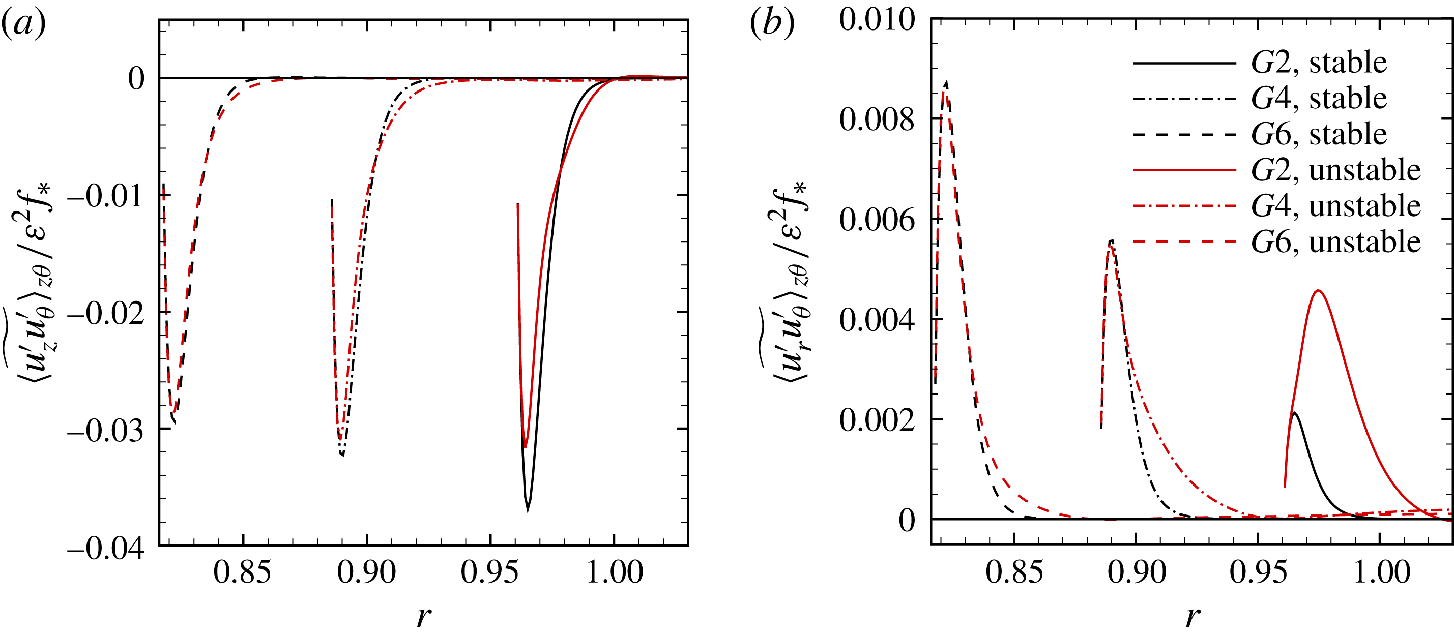
In the statistically stationary state, the azimuthal mean flow is axisymmetric and has reached a balance in the averaged sense. This implies that the terms with the time derivative and those with azimuthal derivatives vanish. The azimuthal (
 $\unicode[STIX]{x1D703}$
) component of the RANS equations in the cylindrical co-rotating frame of reference thus reads
 $$\begin{eqnarray}\displaystyle & & \displaystyle \frac{\langle \widetilde{u}_{\unicode[STIX]{x1D703}}\rangle _{z\unicode[STIX]{x1D703}}\langle \widetilde{u}_{r}\rangle _{z\unicode[STIX]{x1D703}}}{r}+f\langle \widetilde{u}_{r}\rangle _{z\unicode[STIX]{x1D703}}+\langle \widetilde{u}_{r}\rangle _{z\unicode[STIX]{x1D703}}\unicode[STIX]{x2202}_{r}\langle \widetilde{u}_{\unicode[STIX]{x1D703}}\rangle _{z\unicode[STIX]{x1D703}}\approx E\left(\unicode[STIX]{x2202}_{r}^{2}\langle \widetilde{u}_{\unicode[STIX]{x1D703}}\rangle _{z\unicode[STIX]{x1D703}}+\frac{\unicode[STIX]{x2202}_{r}\langle \widetilde{u}_{\unicode[STIX]{x1D703}}\rangle _{z\unicode[STIX]{x1D703}}}{r}-\frac{\langle \widetilde{u}_{\unicode[STIX]{x1D703}}\rangle _{z\unicode[STIX]{x1D703}}}{r^{2}}\right)\nonumber\\ \displaystyle & & \displaystyle \quad -\,\unicode[STIX]{x2202}_{z}\langle \widetilde{u_{z}^{\prime }u_{\unicode[STIX]{x1D703}}^{\prime }}\rangle _{z\unicode[STIX]{x1D703}}-\unicode[STIX]{x2202}_{r}\langle \widetilde{u_{r}^{\prime }u_{\unicode[STIX]{x1D703}}^{\prime }}\rangle _{z\unicode[STIX]{x1D703}}-2\frac{\langle \widetilde{u_{r}^{\prime }u_{\unicode[STIX]{x1D703}}^{\prime }}\rangle _{z\unicode[STIX]{x1D703}}}{r}.\end{eqnarray}$$
There are two remaining Reynolds stress terms in (3.24). One is
 $\langle \widetilde{u_{r}^{\prime }u_{\unicode[STIX]{x1D703}}^{\prime }}\rangle _{z\unicode[STIX]{x1D703}}$
, the other one is
 $\langle \widetilde{u_{z}^{\prime }u_{\unicode[STIX]{x1D703}}^{\prime }}\rangle _{z\unicode[STIX]{x1D703}}$
. Inspecting this equation for the geometry
 $G1$
, for which the boundary layer is a SBL, numerical results reveal that the radial turbulent transport is much larger than the axial one
 $(\langle \widetilde{u_{r}^{\prime }u_{\unicode[STIX]{x1D703}}^{\prime }}\rangle _{z\unicode[STIX]{x1D703}}\gg \langle \widetilde{u_{z}^{\prime }u_{\unicode[STIX]{x1D703}}^{\prime }}\rangle _{z\unicode[STIX]{x1D703}})$
. This case is investigated in detail by Ghasemi et al. (Reference Ghasemi, Klein, Harlander, Kurgansky, Schaller and Will2016, § D), who suggested neglecting the axial transport term.
Present numerical results for cases with the inner cylinder wall tilted with respect to the rotation axis (geometries
 $G2$
–
 $G7$
), however, exhibit a different behaviour, suggesting that the axial Reynolds stress term
 $\langle \widetilde{u_{z}^{\prime }u_{\unicode[STIX]{x1D703}}^{\prime }}\rangle _{z\unicode[STIX]{x1D703}}$
cannot be neglected in comparison to the radial one
 $\langle \widetilde{u_{r}^{\prime }u_{\unicode[STIX]{x1D703}}^{\prime }}\rangle _{z\unicode[STIX]{x1D703}}$
. In these geometries, there is an ESBL over the frustum which causes
 $u_{\unicode[STIX]{x1D703}}^{\prime }$
to be coupled to
 $u_{z}^{\prime }$
in the vicinity of the wall (Ekman property of the ESBL). This results in a larger correlation
 $\langle \widetilde{u_{z}^{\prime }u_{\unicode[STIX]{x1D703}}^{\prime }}\rangle _{z\unicode[STIX]{x1D703}}$
.
Figure 9 shows radial profiles of
 $\langle \widetilde{u_{r}^{\prime }u_{\unicode[STIX]{x1D703}}^{\prime }}\rangle _{z\unicode[STIX]{x1D703}}$
and
 $\langle \widetilde{u_{z}^{\prime }u_{\unicode[STIX]{x1D703}}^{\prime }}\rangle _{z\unicode[STIX]{x1D703}}$
for the stable and unstable ESBLs for the geometries
 $G2$
,
 $G4$
and
 $G6$
and for different
 $\unicode[STIX]{x1D6FC}$
or
 $f_{\ast }$
. As previously, the simulations are done for two different libration amplitudes
 $\unicode[STIX]{x1D700}$
. Assuming that each velocity fluctuation scales with
 $\unicode[STIX]{x1D700}$
and making use of the fact that the Ekman flux depends on
 $f_{\ast }$
, the Reynolds stress terms are scaled with
 $\unicode[STIX]{x1D700}^{2}f_{\ast }$
. (This compensates approximately the empirical mean flow scaling given in (3.23).)
In figure 9(a) one can see that the radial profiles of
 $\langle \widetilde{u_{z}^{\prime }u_{\unicode[STIX]{x1D703}}^{\prime }}\rangle _{z\unicode[STIX]{x1D703}}/(\unicode[STIX]{x1D700}^{2}f_{\ast })$
for the intermittently unstable ESBL approach those of the stable ESBL with increasing
 $f_{\ast }$
(geometries
 $G2$
–
 $G6$
from right to left). For the geometry
 $G2$
, the librational forcing governs the ESBL dynamics (regime (iii)) and there is only a weak Ekman flux. By contrast, there is a considerable Ekman flux parallel to the frustum for the geometries
 $G4$
and
 $G6$
(compare with figure 6). In the cylindrical coordinates, the Ekman flux parallel to the frustum has always components in both the radial and axial directions, although with different magnitude. As
 $f_{\ast }$
increases, the Ekman flux increases, causes
 $u_{z}^{\prime }$
to be increased and results in a larger correlation
 $\langle \widetilde{u_{z}^{\prime }u_{\unicode[STIX]{x1D703}}^{\prime }}\rangle _{z\unicode[STIX]{x1D703}}$
(
 $\langle \widetilde{u_{z}^{\prime }u_{\unicode[STIX]{x1D703}}^{\prime }}\rangle _{z\unicode[STIX]{x1D703}}^{min}=-0.0024$
for
 $G2$
, but
 $-0.010$
for
 $G6$
). In figure 9(b) and for the geometry
 $G2$
(regime (iii)) one can see that
 $\langle \widetilde{u_{r}^{\prime }u_{\unicode[STIX]{x1D703}}^{\prime }}\rangle _{z\unicode[STIX]{x1D703}}/(\unicode[STIX]{x1D700}^{2}f_{\ast })$
is larger for the unstable ESBL compared to the stable ESBL. As
 $f_{\ast }$
increases (
 $G2$
–
 $G6$
, from right to left), the radial profile of the radial Reynolds stress term of the unstable ESBL approaches that of the stable ESBL. For the geometry
 $G6$
(regime (ii)) those profiles almost coincide again.
Note that the radial profiles shown in figure 9(a,b) are notably different for the stable and unstable ESBL. This is most notable for the geometry
 $G2$
with weakest
 $f_{\ast }$
. As we saw already in figure 6(b), the Ekman flux is weak and therefore substantially perturbed by the Görtler vortices. This seems to explain also the differences seen in the Reynolds stresses. Following Ghasemi et al. (Reference Ghasemi, Klein, Harlander, Kurgansky, Schaller and Will2016, §§ C and D), the Görtler vortices generate a mean flow due to the radial gradient of
 $\langle \widetilde{u_{r}^{\prime }u_{\unicode[STIX]{x1D703}}^{\prime }}\rangle _{z\unicode[STIX]{x1D703}}$
outside of the boundary layer in the case of an inner straight cylinder (geometry
 $G1$
). In the geometry
 $G2$
the situation does not change much implying that the Görtler vortices have a considerable influence on the mean flow in the vicinity of the ESBL. However, as
 $f_{\ast }$
increases, the ESBL becomes thicker and the vortices need to travel further within the boundary layer (see § 3.6). In the geometry
 $G6$
, this effect seems responsible for a smaller contribution of the Görtler vortices to the term
 $\langle \widetilde{u_{r}^{\prime }u_{\unicode[STIX]{x1D703}}^{\prime }}\rangle _{z\unicode[STIX]{x1D703}}$
outside the boundary layer and, consequently, causes the mean flow to be diminished.
Note further that in the case of the stable ESBL there are no Görtler vortices. Nevertheless, there is considerable overlap of the profiles corresponding to the geometry
 $G6$
shown in figure 9(b). We attribute this contribution to the mean flow to the Ekman flux through the corner flow at the bottom which is now responsible for generating
 $\langle \widetilde{u_{r}^{\prime }u_{\unicode[STIX]{x1D703}}^{\prime }}\rangle _{z\unicode[STIX]{x1D703}}$
.
On the basis of numerical data we performed a scale analysis with the cylindrical RANS equation (3.24). We kept only those terms larger than a threshold of
 $5\,\%$
of the largest term. In addition, the
 $1/r$
-terms where neglected in favour of the radial derivatives because we are facing an azimuthal jet and this jet is relatively thin compared to the annular gap (this is analogous to Ghasemi et al.
Reference Ghasemi, Klein, Harlander, Kurgansky, Schaller and Will2016, §§ D and E). So, with these simplifications in (3.24) we obtain the empirical balance
 $$\begin{eqnarray}\displaystyle \underbrace{\unicode[STIX]{x2202}_{r}\langle \widetilde{u_{r}^{\prime }u_{\unicode[STIX]{x1D703}}^{\prime }}\rangle _{z\unicode[STIX]{x1D703}}}_{RT}+\underbrace{\unicode[STIX]{x2202}_{z}\langle \widetilde{u_{z}^{\prime }u_{\unicode[STIX]{x1D703}}^{\prime }}\rangle _{z\unicode[STIX]{x1D703}}}_{AT}+\underbrace{f\langle \widetilde{u}_{r}\rangle _{z\unicode[STIX]{x1D703}}}_{LA}\approx \underbrace{E\unicode[STIX]{x2202}_{r}^{2}\langle \widetilde{u}_{\unicode[STIX]{x1D703}}\rangle _{z\unicode[STIX]{x1D703}}}_{D}, & & \displaystyle\end{eqnarray}$$
where
 $RT$
is the radial turbulent transport,
 $AT$
is the axial turbulent transport,
 $LA$
is the local Coriolis force affecting the azimuthal balance and
 $D$
is the viscous diffusion. Equation (3.25) is an approximate balance for which the validity has been proven numerically as will be discussed shortly. In view of this, it is not surprising to see in figure 8(a–d) that the radial derivative dominates the viscous terms and that the Coriolis force has a notable contribution only due to the azimuthal mean flow. Note that the turbulent axial transport term
 $AT$
was not present in the diagnostic RANS equation for the straight annulus (geometry
 $G1$
; see Ghasemi et al.
Reference Ghasemi, Klein, Harlander, Kurgansky, Schaller and Will2016). We therefore conjecture that
 $AT$
is also related to the Ekman property of the ESBL which manifests itself otherwise mainly by driving the Ekman flux up and down the frustum wall.
Radial profiles of the terms contributing to the approximate balance (3.25) for the geometries
 $G2$
in regime (iii) (a) and
 $G6$
in regime (ii) (b) for the intermittently unstable ESBL. The contributions shown are the turbulent axial and radial transport terms (
 $AT$
and
 $RT$
), the Coriolis force (
 $LA$
), the viscous diffusion (
 $D$
) and the balance as the difference of the right- minus left-hand side (
 $R-L$
). The ESBL thickness
 $\unicode[STIX]{x1D6FF}$
is given for orientation and corresponds to the laminar value
 $\unicode[STIX]{x1D6FF}_{-}$
according to equation (3.6).
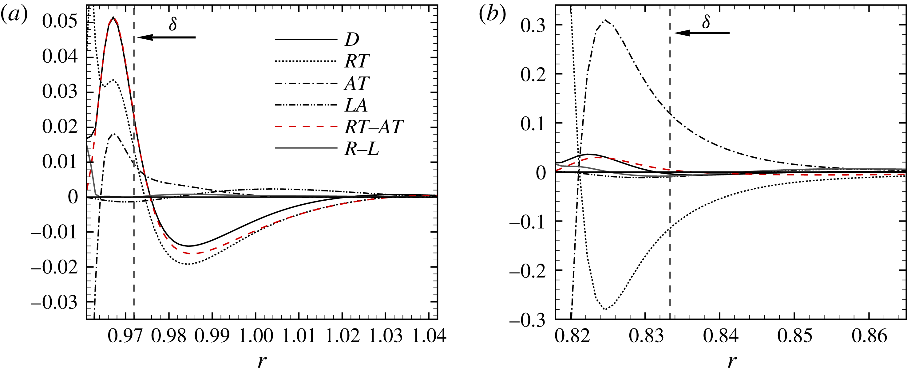
Figure 10 shows the radial profiles of the different terms given in (3.25) for the case of an unstable ESBL in the geometries
 $G2$
and
 $G6$
corresponding to the flow regimes (iii) and (ii), respectively. In figure 10(a), one can see that
 $RT$
is almost balanced by
 $D$
for the geometry
 $G2$
. As we discussed at the beginning of this section, the situation for the geometry
 $G2$
is very close to the geometry
 $G1$
and the term
 $AT$
is generally weak since it is related to the Ekman flux, which is weak here, too. This is in agreement with the previous discussion of figure 8 where we concluded that, for the geometry
 $G2$
, the prograde mean flow for the unstable ESBL is mainly due to the Görtler vortices. For the geometry
 $G6$
the magnitudes of
 $RT$
and
 $AT$
are very similar outside of the ESBL, but both terms have opposite signs and their magnitude is much larger than that of
 $D$
. Therefore, one can argue that in (3.25)
 $RT$
takes the role of a generating agent, whereas
 $AT$
takes that of a destructing agent for the prograde mean flow. This argument is supported also by figure 8, in which we saw that the prograde azimuthal mean flow is actually missing over the largest part of the frustum for the geometry
 $G6$
. Instead, only a prograde jet was originating from the bottom corner.
Note that the positive sign of the mean flow driven by an unstable ESBL can also be understood with the aid of (3.25). The negative sign of
 $RT$
outside of the boundary layer implies generation of a positive (prograde) mean flow. This is fully analogous to Ghasemi et al. (Reference Ghasemi, Klein, Harlander, Kurgansky, Schaller and Will2016, § D).
4 Summary and conclusion
In this paper we have used direct numerical simulations (DNS) to study an intermittently unstable boundary layer flow over a conical wall (frustum). The frustum forms the inner wall of an annular confinement, which is filled with an incompressible Newtonian fluid of kinematic viscosity
 $\unicode[STIX]{x1D708}$
, and we consider the whole set-up to rotate uniformly with mean angular velocity
 $\unicode[STIX]{x1D6FA}_{0}$
. The annular configuration studied models the near equator and mid-latitudes of planetary-scale flows, which means that results obtained are generally relevant for geophysical applications, like core and mantle flows, but also for the ocean or even the atmosphere. Flows have been excited by longitudinal libration i.e. by a sinusoidal modulation of the rotation rate of the inner wall. The libration frequency was kept fixed at
 $\unicode[STIX]{x1D714}=\unicode[STIX]{x1D6FA}_{0}$
but two different values of the libration amplitude
 $\unicode[STIX]{x1D700}\unicode[STIX]{x1D6FA}_{0}$
have been investigated. These yield stable (
 $\unicode[STIX]{x1D700}=0.2$
) and intermittently unstable (
 $\unicode[STIX]{x1D700}=0.8$
) flow conditions for the selected Ekman number
 $E=\unicode[STIX]{x1D708}/(\unicode[STIX]{x1D6FA}_{0}r_{1}^{2})=4\times 10^{-5}$
with
 $r_{1}$
the maximum frustum radius.
An important aspect of the present work concerns the dependency of the stable and unstable flow on the wall inclination angle
 $\unicode[STIX]{x1D6FC}$
measured relative to the rotation axis. Guided by the notion that the flow remains stable for small libration amplitudes, we used laminar boundary layer theory to obtain analytical expressions for the velocity field. The wall inclination enters through the local Coriolis parameter
 $f_{\ast }=2\unicode[STIX]{x1D6FA}_{0}\sin \unicode[STIX]{x1D6FC}$
, which means that the solution presented may potentially be useful also for spherical geometry for which
 $f_{\ast }$
is not constant but varies with latitude. Our analytical analysis accounts schematically for wall curvature by adopting the vorticity-divergence form so that the radial dependency of the wall velocity can be accounted for in the vorticity boundary condition in an otherwise Cartesian treatment.
The boundary layer solution yields the presence of an Ekman–Stokes boundary layer (ESBL), which is characterized by an along wall (axial–radial) velocity representing an oscillating oblique mass flux along the frustum wall (Ekman property), and an oscillatory azimuthal velocity representing a kind of damped wave which follows the wall libration (Stokes property). The key similarity parameter of the ESBL is the time scale ratio
 $\unicode[STIX]{x1D6FE}=\unicode[STIX]{x1D714}/f_{\ast }$
. According to
 $\unicode[STIX]{x1D6FE}$
, three different flow regimes have been identified: (i) rotation dominated (
 $\unicode[STIX]{x1D6FE}\ll 1$
), (ii) rotation–libration dominated (
 $\unicode[STIX]{x1D6FE}\sim 1$
) and (iii) libration dominated (
 $\unicode[STIX]{x1D6FE}\gg 1$
). The flow regimes (ii) and (iii) have been studied in this work by variation of the local Coriolis parameter
 $f_{\ast }$
through the wall inclination
 $\unicode[STIX]{x1D6FC}$
. The configuration in which the inner wall is parallel to the rotation axis (
 $\unicode[STIX]{x1D6FC}=0$
) comprises an extreme situation in which a pure Stokes boundary layer (SBL) is established over the librating wall. As the inclination angle increases, the Ekman property of the ESBL becomes more important until, finally, rotation dominates the boundary layer dynamics (
 $\unicode[STIX]{x1D6FE}\ll 1$
). A comparison of our 1-D boundary layer solution to stable 3-D DNS results far away from the lids exhibits very good agreement with respect to instantaneous velocities. This suggests the presence of an ESBL in the DNS results. The wall-normal velocity component is driven by the vortical boundary condition and compares less well. We attribute this to wall curvature and other geometrical effects (like end plates). However, the magnitude of the wall-normal velocity over the librating wall is
 $3$
–
 $4$
orders of magnitude smaller than the wall-tangential velocities of the ESBL. Interestingly, the wall-tangential velocities turn out comparable to the solution given by Salon & Armenio (Reference Salon and Armenio2011), who considered a tidally driven flow in the first place. Their solution is the limiting case of our solution for a very large wall curvature radius.
With an understanding of the laminar ESBL properties we moved on to gain a better understanding of the intermittently unstable flow. The intermittency is imposed here by wall libration, which yields alternating Rayleigh-stable and Rayleigh-unstable conditions near the wall. The ESBL turns centrifugally unstable when the wall starts to decelerate (
 $\unicode[STIX]{x1D714}t=\unicode[STIX]{x03C0}/2$
), but libration amplitudes have to be large-enough to let the instability grow before the flow stabilizes again near the wall. For the SBL over a straight cylinder it is the induced azimuthal flow plus curvature which yield the Görtler-type instability (Sauret et al.
Reference Sauret, Cébron, Le Bars and Le Dizès2012; Ghasemi et al.
Reference Ghasemi, Klein, Harlander, Kurgansky, Schaller and Will2016). Results presented suggest that this argumentation can be carried over to the ESBL, especially when the wall inclination is weak.
Indeed, the presented DNS results exhibit a qualitative similarity of the ESBL instability to that of the SBL, say a formation of elongated Görtler vortices near the wall. However, these vortices are tilted compared to the azimuthal coordinate in the ESBL over the frustum, whereas they are azimuthally aligned in the SBL over a straight cylinder. We suggest that the instability develops in locally close-to-laminar flow conditions and use the laminar boundary layer theory to study the flow at the libration phase when the instability develops. It turns out that the ESBL exhibits an oblique mass flux along the frustum wall (Ekman flux) due to the Coriolis force, which is absent in the SBL. Consequently, it is this oblique flow over the frustum wall at onset of instability which causes the tilt of the Görtler vortices. This simply shows how the Ekman property of the ESBL influences the Stokes property of the ESBL. In turn, the Ekman flux in the retrograde phase is also affected by the development of the vortices which is more visible for smaller inclination angles (figure 9).
The latter explanation regarding the origin of the tilt of the Görtler vortices is supported by the stress angle
 $\unicode[STIX]{x1D6FD}_{\unicode[STIX]{x1D70F}}$
, which measures the direction of the wall shear stress relative to the azimuthal coordinate. The wall shear stress depends strongly on the mass flux in the boundary layer. Both quantities are therefore coupled. Furthermore, the ratio of the wall shear stress components
 $|\unicode[STIX]{x1D70F}_{\unicode[STIX]{x1D703}}|_{+}^{max}/|\unicode[STIX]{x1D70F}_{\Vert }|_{+}^{max}$
was found to scale almost linearly with
 $\unicode[STIX]{x1D6FE}$
. This implies that it can be used as a substitute for the
 $\unicode[STIX]{x1D6FE}$
parameter for identification of the flow regime which can be useful for applications. Coming back to the stress angle, it turns out that
 $\unicode[STIX]{x1D6FD}_{\unicode[STIX]{x1D70F}}$
follows roughly the tilt
 $\unicode[STIX]{x1D6FD}$
of the Görtler vortices which means there is only a weak dependency on the wall inclination
 $\unicode[STIX]{x1D6FC}$
itself since
 $\unicode[STIX]{x1D6FD}_{\unicode[STIX]{x1D70F}}/\unicode[STIX]{x1D6FD}\approx 1$
. We conclude that the laminar boundary layer dynamics is crucial for an understanding of the unstable ESBL and the developing Görtler instability. Here it is the linear dynamics (Coriolis force and Ekman flux) in combination with wall curvature (centrifugal instability) that is responsible for the deflection of the Görtler vortices over the librating frustum.
Note further that the effective curvature radius for the laminar boundary layer flow increases with the wall inclination angle
 $\unicode[STIX]{x1D6FC}$
. This is revealed also by a non-zero stress angle at the most unstable libration phase. We conjecture that there is a critical inclination angle
 $\unicode[STIX]{x1D6FC}_{c}$
for the Görtler instability to occur for a selected wall curvature radius, libration frequency, libration amplitude and Ekman number, but this has to be addressed in a future study.
An interesting feature of the bulk flow in the case of the stable ESBL is to be seen in a prograde azimuthal jet, which is coaxially aligned with the rotation axis and present over the librating inner wall. More precisely, the prograde jet originates from the bottom corner and extends up to the top lid. The prograde jet seems to be a reminiscent of the Stewartson layer in a librating spherical shell and has a linear dependency on
 $\unicode[STIX]{x1D700}^{2}f_{\ast }$
. For the intermittently unstable ESBL, the development of the Görtler vortices not only affects the ESBL but also the fluid bulk. An additional prograde mean flow is generated in the bulk which we attribute to the angular momentum transport induced by the Görtler vortices. This mean flow, however, does not exhibit the scaling
 $\unicode[STIX]{x1D700}^{2}f_{\ast }$
of the stable ESBL (see figure 8
f).
We investigated the scaling of the mean flow related to the Görtler vortices by varying the wall inclination. Increasing the inclination angle towards the axial direction led to a reduction of the magnitude of the prograde mean flow. In other words, the mean flow magnitude decreased with the tilt of the Görtler vortices. Furthermore, for a small wall inclination (geometry
 $G2$
in regime (iii)), we saw approximately an order of magnitude jump in the prograde mean flow amplitude when the ESBL was changed from stable to unstable flow conditions. Increasing the wall inclination towards geometry
 $G7$
in regime (ii) leads to a larger tilt of the Görtler vortices and some thickening of the ESBL. The thickening of the ESBL implies that the Görtler vortices travel further within the boundary layer and decay there before reaching the bulk. Consequently, as
 $\unicode[STIX]{x1D6FC}$
increases from
 $3^{\circ }$
(geometry
 $G2$
) to
 $18^{\circ }$
(geometry
 $G7$
), the magnitude of the prograde azimuthal mean flow related to the Görtler vortices decreases until it has almost vanished in geometry
 $G7$
.
In order to clarify the mean flow generation mechanism due to Görtler vortices over an inclined wall we investigated the azimuthal component of the Reynolds-averaged Navier–Stokes (RANS) equations. We derived at the balance (3.25). In contrast to the diagnostic RANS equation for the straight annulus (Ghasemi et al.
Reference Ghasemi, Klein, Harlander, Kurgansky, Schaller and Will2016), which contains only the generating radial transport
 $RT=\unicode[STIX]{x2202}_{r}\langle \widetilde{u_{r}^{\prime }u_{\unicode[STIX]{x1D703}}^{\prime }}\rangle _{z\unicode[STIX]{x1D703}}$
, we found an additional axial transport term
 $AT=\unicode[STIX]{x2202}_{z}\langle \widetilde{u_{z}^{\prime }u_{\unicode[STIX]{x1D703}}^{\prime }}\rangle _{z\unicode[STIX]{x1D703}}$
, which acts as a destructive agent.
 $AT$
is related to the oblique boundary layer mass flux along the frustum wall (Ekman property of the ESBL) and is not relevant for the SBL over a librating straight cylinder. For the geometry
 $G2$
in which the librational forcing dominates the ESBL dynamics (regime (iii)),
 $RT$
is substantially larger than
 $AT$
outside the ESBL. However, with increasing wall inclination
 $\unicode[STIX]{x1D6FC}$
, the effect of rotation becomes more and more important, and for the geometry
 $G6$
(
 $\unicode[STIX]{x1D6FC}=15^{\circ }$
) the generating agent
 $RT$
is almost entirely balanced by the destructive agent
 $AT$
, preventing the generation of a prograde mean flow. To summarize, the generation mechanism of the azimuthal mean flow by the Görtler vortices in the straight wall annulus (geometry
 $G1$
) was realized by Ghasemi et al. (Reference Ghasemi, Klein, Harlander, Kurgansky, Schaller and Will2016) as the pumping of angular momentum from the boundary layer to the fluid bulk. Here we found that the Ekman property of the ESBL weakens this pumping.
We close by noting that the mean flow generation over an inclined wall discussed above might also be of relevance for the mean flow generation in spherical geometries. There, however, the inclination angle changes with latitude. Our analysis hence shows how the unstable SBL of the equatorial region of a librating spherical shell transits to an ESBL in mid-latitudes and to an eventually stable Ekman layer in the polar regions. The development of the Görtler vortices around the equatorial region of a sphere is known since the early experimental work by Aldridge (Reference Aldridge1967) and the recent experimental and numerical work by Noir et al. (Reference Noir, Hemmerlin, Wicht, Baca and Aurnou2009). The results discussed in the present work propose the generation of an azimuthal mean flow by the Görtler vortices, in addition to the excitation due to interactions within the laminar boundary layer reported by Sauret & Le Dizès (Reference Sauret and Le Dizès2013). Obviously, the equatorial boundary layer does not only erupt for low libration frequencies, it is also prone for Görtler instability due to the SBL property. Our findings demonstrate that strong mean flows and jets cannot only persist in turbulent flows but can even become particularly strong due to turbulence. This result can help to understand long-lived jets in planets and moons by means that the intermittent instability of the ESBL provides an interesting mechanism for maintaining an azimuthal jet under unstable flow conditions. These conditions can be established by libration (as modelled here), but can also be the result of a tidally driven flow that constitutes a similar mathematical problem (Salon & Armenio Reference Salon and Armenio2011). The mean flow driven by the developing Görtler instability of the ESBL is relevant because it is large scale, has constant sign and is of second order (
 $O(\unicode[STIX]{x1D700}^{2})$
, see Ghasemi et al.
Reference Ghasemi, Klein, Harlander, Kurgansky, Schaller and Will2016), which is comparable to the mean flow driven by the nonlinearity of the Ekman layer (Wang Reference Wang1970; Busse Reference Busse2010, Reference Busse2011). Compared to the DNS presented using an Ekman number of
 $4\times 10^{-5}$
, in geophysical flows, shear-related instabilities like the discussed Görtler instability can be expected to become more important due to larger shear resulting from very small Ekman numbers (
 $E\lesssim 10^{-9}$
).
Acknowledgements
The authors wish to thank Michael V. Kurgansky (Russian Academy of Sciences, Moscow, Russian Federation) for providing fruitful comments on the early version of the paper. A.G. thanks the Graduate Research School (GRS) of the Brandenburg University of Technology (BTU) Cottbus-Senftenberg for partially supporting the work. Part of the work was carried out at the Hans Ertel Centre for Weather Research, which is the German research network of Universities, Research Institutes and the German Weather Service (DWD) funded by the Federal Ministry of Transport and Digital Infrastructure (BMVI). U.H. acknowledges financial support from the German Research Foundation (DFG) in the frame of the MS-GWaves project ‘Spontaneous imbalance’ (HA 2932/8-1).
Supplementary material
We would like to mention that processed data (like mean flow profiles) are available on the institutional https://www.b-tu.de/fg-meteorologie/projekte/projekte/laufende-projekte/qbo#c84358 of the Dept. of Environmental Meteorology of the BTU Cottbus-Senftenberg. The numerical solver can be made available on request. It is planned to evaluate our theoretical results with corresponding laboratory measurements in a future study.



