1 Introduction
Vortices are coherent structures in a fluid flow, and much of basic fluid dynamics research is focused on understanding their dynamics, interaction, creation and destruction. By our intuitive understanding, it might not be difficult to identify a strong vortex in a flow. It is, however, harder to locate its boundaries and to explain how it was created. To answer these questions, we need a precise mathematical definition of a vortex. There are many different vortex criteria available in the literature (see Zhang et al. (Reference Zhang, Liu, Xian and Du2018) for a review) and new ideas are continuously being proposed (e.g. Haller et al.
Reference Haller, Hadjighasem, Farazmand and Huhn2016; Zhong et al.
Reference Zhong, Chen, Chen and Li2017). Each of these criteria identifies different structures as vortices, and as yet there is no generally accepted definition of a vortex. In the present paper, we identify vortices based on the widely used
 $Q$
-criterion (Hunt, Wray & Moin Reference Hunt, Wray and Moin1988). The
 $Q$
-criterion locates regions in a flow where the rotation dominates the strain. Like a variety of other Galilean-invariant vortex criteria, it is based on a decomposition of the velocity gradient tensor,
 $\unicode[STIX]{x1D735}\boldsymbol{u}$
. In its general form,
 $Q$
is defined as the following measure of stretching relative to rotation,
 $$\begin{eqnarray}Q={\textstyle \frac{1}{2}}(\Vert \unicode[STIX]{x1D734}\Vert ^{2}-\Vert \unicode[STIX]{x1D64E}\Vert ^{2}),\end{eqnarray}$$
where
 $\unicode[STIX]{x1D64E}={\textstyle \frac{1}{2}}(\unicode[STIX]{x1D735}\boldsymbol{u}+\unicode[STIX]{x1D735}\boldsymbol{u}^{\text{T}})$
is the symmetric strain-rate tensor,
 $\unicode[STIX]{x1D734}={\textstyle \frac{1}{2}}(\unicode[STIX]{x1D735}\boldsymbol{u}-\unicode[STIX]{x1D735}\boldsymbol{u}^{\text{T}})$
is the skew-symmetric vorticity tensor and
 $\Vert \unicode[STIX]{x1D653}\Vert =\sqrt{\text{tr}(\unicode[STIX]{x1D653}\unicode[STIX]{x1D653}^{\text{T}})}$
. The criterion defines a vortex as a region with positive
 $Q$
-value. In a two-dimensional setting the
 $Q$
-criterion is equivalent to other frequently used vortex criteria such as the
 $\unicode[STIX]{x1D6E5}$
-criterion, the
 $\unicode[STIX]{x1D706}_{2}$
-criterion (Jeong & Hussain Reference Jeong and Hussain1995) and the
 $\unicode[STIX]{x1D706}_{ci}$
-criterion (Zhou et al.
Reference Zhou, Adrian, Balachandar and Kendall1999). All of these simplify to the determinant of the velocity gradient being positive, i.e.
 $$\begin{eqnarray}Q(x,y)=\det (\unicode[STIX]{x1D735}\boldsymbol{u}(x,y))>0.\end{eqnarray}$$
In practice, it is common to choose a non-zero threshold to identify the vortex boundaries. The threshold is ideally chosen such that strong vortices are captured while small spurious vortices (e.g. those arising as artefacts in data from numerical simulations) are ignored. Unfortunately, it is very difficult, if not impossible, to determine a suitable threshold value a priori because the optimal threshold value tends to be problem-dependent (see Chakraborty, Balachandar & Adrian Reference Chakraborty, Balachandar and Adrian2005; Chen et al.
Reference Chen, Zhong, Qi and Wang2015). In this paper we therefore consider the
 $Q$
-criterion with zero threshold as defined in (1.2).
Having established a criterion that identifies vortices in a precise mathematical way, we employ bifurcation theory to analyse the conditions under which vortices are created, destroyed, merge or split. This is done by considering
 $Q$
as a function of time
 $t$
, which we treat as the primary bifurcation parameter. The main result of our studies is a detailed analysis of the creation, destruction or merging of vortices in terms of changes in the topology of the level set
 $Q=0$
. Previous topological studies of bifurcations of structures in flows have focused on critical points for either the velocity (see e.g. Brøns Reference Brøns2007; Balci et al.
Reference Balci, Andersen, Thompson and Brøns2015) or the vorticity (Brøns & Bisgaard Reference Brøns and Bisgaard2006; Heil et al.
Reference Heil, Rosso, Hazel and Brøns2017). Here we are concerned with bifurcations of curves rather than critical points, and a different mathematical approach is needed. The overall strategy is, however, the same: a bifurcation is characterized by a number of degeneracy conditions which state that certain combinations of derivatives of
 $Q$
must be zero. These are combined with non-degeneracy conditions, which are inequalities ensuring that certain higher-order derivatives are non-zero. The degeneracy conditions are equations that make it possible to locate a bifurcation point. To be able to determine where in space and time a certain bifurcation occurs, three degeneracy conditions are needed. The non-degeneracy conditions ensure a certain regularity of the
 $Q$
function allowing us to employ the implicit function theorem to determine the properties of the level curve
 $Q=0$
close to the bifurcation point. The bifurcations obtained in this way are denoted codimension-one bifurcations. If an additional parameter, such as the Reynolds number
 $Re$
, is varied, one of the non-degeneracy conditions may be violated at a given value of that parameter. Subject to further non-degeneracy conditions, a two-parameter bifurcation diagram can be established, and the bifurcation is then said to have codimension two. Adding more parameters, this procedure can then be repeated, but the number of possible bifurcations and the complexity of the bifurcation diagrams increase rapidly with the codimension.
In the present paper we obtain a complete list of codimension-one bifurcations. There are four types: pinching and punching bifurcations occur away from boundaries, while wall-pinching and wall-punching are bifurcations of vortices attached to a no-slip wall.
To illustrate how our theory can be used, we apply it to the classical fluid mechanics problem of boundary layer eruption. In this problem a large vortex is convected close to a no-slip wall. This vortex induces vorticity in the boundary layer which may, or may not, erupt and form secondary vortices. This process has previously been studied by Doligalski & Walker (Reference Doligalski and Walker1984), Obabko & Cassel (Reference Obabko and Cassel2002), Kudela & Malecha (Reference Kudela and Malecha2009) and Andersen (Reference Andersen2013) among others. We consider the early stages of boundary layer eruption at moderate
 $Re$
. By tracking the flow structures for fixed
 $Re$
, we show that our approach allows a rigorous description of the creation of vortices as a series of bifurcations of the zero contours of
 $Q$
. The bifurcations are generally of codimension one, but a single codimension-two point is found. The corresponding value of
 $Re$
marks a change in the topology of the vortex pattern, and in an appendix we provide a detailed analysis of this case.
2 Bifurcations of
 $Q=0$
curves away from boundaries

We start by considering a region of fluid which is not in the vicinity of any boundary. Our goal is to characterize the conditions under which we see topological changes in the local structure of the zero contour curves of
 $Q$
. As a starting point we consider a non-critical point on the zero contour curve, i.e. a point
 $(x^{\ast },y^{\ast },t^{\ast })$
, where
 $$\begin{eqnarray}Q(x^{\ast },y^{\ast },t^{\ast })=0\end{eqnarray}$$
and
 $$\begin{eqnarray}\unicode[STIX]{x2202}_{x}Q(x^{\ast },y^{\ast },t^{\ast })\neq 0\quad \text{or}\quad \unicode[STIX]{x2202}_{y}Q(x^{\ast },y^{\ast },t^{\ast })\neq 0.\end{eqnarray}$$
In the case where
 $\unicode[STIX]{x2202}_{x}Q(x^{\ast },y^{\ast },t^{\ast })$
is non-zero, it follows from the implicit function theorem that there exist a unique local function
 $X(y,t)=x$
satisfying
 $X(y^{\ast },t^{\ast })=x^{\ast }$
and
 $Q(X(y,t),y,t)=0$
. The uniqueness of
 $X$
implies that we only have a single zero contour curve close to
 $(x^{\ast },y^{\ast })$
at time
 $t=t^{\ast }$
. Furthermore, the continuity of
 $X$
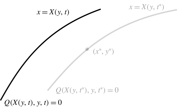
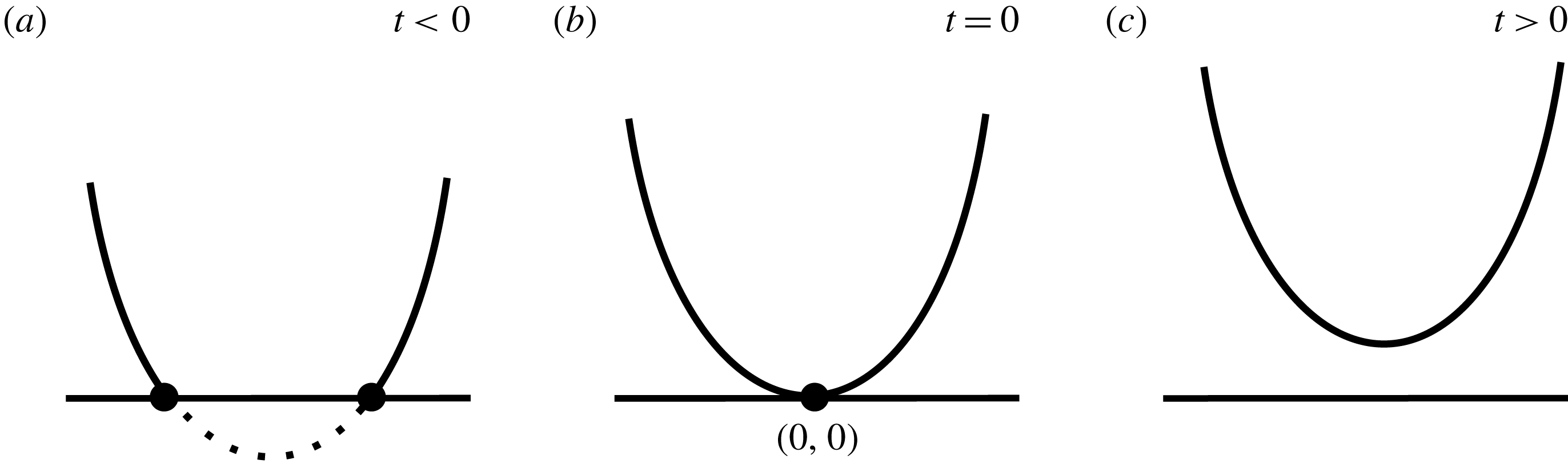
guarantees that the zero contour curve will not change its topological structure for any sufficiently small changes in time, as illustrated in figure 1. We therefore conclude that
 $(x^{\ast },y^{\ast })$
cannot be a bifurcation point at time
 $t^{\ast }$
. If we consider the case where
 $\unicode[STIX]{x2202}_{x}Q(x^{\ast },y^{\ast },t^{\ast })=0$
, we can give a completely similar argument based on the fact that
 $\unicode[STIX]{x2202}_{y}Q(x^{\ast },y^{\ast },t^{\ast })$
is non-zero. This implies that we must look for critical points of
 $Q$
to identify any possible bifurcation points on the zero contour curve.
Illustration of how a small change in time away from
 $t^{\ast }$
affects the topological structure of the contour curve,
 $Q=0$
, close to a non-critical point
 $(x^{\ast },y^{\ast })$
. Since the topological structure is unchanged,
 $(x^{\ast },y^{\ast })$
is not a bifurcation point.

For simplicity, we choose a coordinate system such that the critical point is located at
 $(x,y)=(0,0)$
at time
 $t=0$
and we use subscript
 $0$
to denote any function evaluation at
 $(x,y,t)=(0,0,0)$
. Based on the discussion above, bifurcation points must fulfil
 $$\begin{eqnarray}Q_{0}=0,\quad \unicode[STIX]{x2202}_{x}Q_{0}=0,\quad \unicode[STIX]{x2202}_{y}Q_{0}=0.\end{eqnarray}$$
If the Hessian matrix is non-singular at
 $(x,y,t)=(0,0,0)$
, it can be used to classify the type of critical point. Hence we take as the first non-degeneracy condition
 $$\begin{eqnarray}H_{0}^{Q}=\left(\begin{array}{@{}cc@{}}\unicode[STIX]{x2202}_{xx}Q_{0} & \unicode[STIX]{x2202}_{xy}Q_{0}\\ \unicode[STIX]{x2202}_{xy}Q_{0} & \unicode[STIX]{x2202}_{yy}Q_{0}\end{array}\right)\text{ is non-singular}.\end{eqnarray}$$
As the second non-degeneracy condition we assume
 $$\begin{eqnarray}\unicode[STIX]{x2202}_{t}Q_{0}\neq 0,\end{eqnarray}$$
which will be needed to apply the implicit function theorem later in the analysis.
Based on the above assumptions, we will now show that a bifurcation occurs at
 $(x,y,t)=(0,0,0)$
. Applying that
 $Q_{0}=0$
and
 $\unicode[STIX]{x2202}_{t}Q_{0}\neq 0$
, it follows from the implicit function theorem that there exists a unique local function
 $T(x,y)=t$
satisfying that
 $T_{0}=T(0,0)=0$
and
 $Q(x,y,T(x,y))=0$
. The equation
 $t=T(x,y)$
, for a given
 $t$
, will therefore determine the zero contour curve of
 $Q$
at that time. In order to characterize the topological structure of the contour curves, we need some properties of the function
 $T$
. By implicit differentiation of
 $Q$
, we obtain that
 $$\begin{eqnarray}\unicode[STIX]{x2202}_{x}T_{0}=-{\displaystyle \frac{\unicode[STIX]{x2202}_{x}Q_{0}}{\unicode[STIX]{x2202}_{t}Q_{0}}}=0,\quad \unicode[STIX]{x2202}_{y}T_{0}=-{\displaystyle \frac{\unicode[STIX]{x2202}_{y}Q_{0}}{\unicode[STIX]{x2202}_{t}Q_{0}}}=0\end{eqnarray}$$
and the Hessian
 $$\begin{eqnarray}H_{0}^{T}=\left(\begin{array}{@{}cc@{}}\unicode[STIX]{x2202}_{xx}T_{0} & \unicode[STIX]{x2202}_{xy}T_{0}\\ \unicode[STIX]{x2202}_{xy}T_{0} & \unicode[STIX]{x2202}_{yy}T_{0}\end{array}\right)=-{\displaystyle \frac{1}{\unicode[STIX]{x2202}_{t}Q_{0}}}H_{0}^{Q}.\end{eqnarray}$$
Equation (2.6) shows that
 $(x,y)=(0,0)$
is a critical point for
 $T$
. Since
 $\unicode[STIX]{x2202}_{t}Q_{0}$
is non-zero and
 $H_{0}^{Q}$
is non-singular, it follows from (2.7) that
 $H_{0}^{T}$
is also non-singular and the critical point is therefore a saddle point, a local maximum or a local minimum. With these conditions, we can apply the Morse lemma (Wiggins Reference Wiggins2003) on
 $T$
and conclude that in a neighbourhood of the critical point there exists a (possibly nonlinear) coordinate change,
 $\hat{x}=\hat{x}(x,y)$
,
 ${\hat{y}}={\hat{y}}(x,y)$
, such that
 $$\begin{eqnarray}\hat{x}(0,0)=0,\quad {\hat{y}}(0,0)=0\end{eqnarray}$$
and
 $$\begin{eqnarray}\displaystyle & \displaystyle T(\hat{x},{\hat{y}})=\hat{x}^{2}+{\hat{y}}^{2}\quad \text{if }H_{0}^{T}\text{ is positive definite,} & \displaystyle\end{eqnarray}$$
 $$\begin{eqnarray}\displaystyle & \displaystyle T(\hat{x},{\hat{y}})=-\hat{x}^{2}-{\hat{y}}^{2}\quad \text{if }H_{0}^{T}\text{ is negative definite,} & \displaystyle\end{eqnarray}$$
 $$\begin{eqnarray}\displaystyle & \displaystyle T(\hat{x},{\hat{y}})=\hat{x}^{2}-{\hat{y}}^{2}\quad \text{if }H_{0}^{T}\text{ is indefinite.} & \displaystyle\end{eqnarray}$$
 $T$
. We now consider these cases in separate sections.
2.1
$H_{0}^{Q}$
definite: punching bifurcation

Illustration of the local changes in structure of the
 $Q=0$
contour curve during a punching bifurcation. The figure shows the forward version where
 $\text{sign}(\unicode[STIX]{x2202}_{t}Q_{0})\neq \text{sign}(\text{tr}(H_{0}^{Q}))$
. At the bifurcation value
 $t=0$
,
 $(0,0)$
is the only point where
 $Q=0$
.

First we consider the case where
 $H_{0}^{Q}$
is positive or negative definite. We see from (2.7) that
 $H_{0}^{T}$
is definite as well. In order to determine if
 $H_{0}^{T}$
is positive or negative definite, we consider the sign of the trace of
 $H_{0}^{T}$
,
 $$\begin{eqnarray}\text{sign}(\text{tr}(H_{0}^{T}))=-\text{sign}(\unicode[STIX]{x2202}_{t}Q_{0})\,\text{sign}(\text{tr}(H_{0}^{Q})).\end{eqnarray}$$
In the case where
 $\text{sign}(\unicode[STIX]{x2202}_{t}Q_{0})\neq \text{sign}(\text{tr}(H_{0}^{Q}))$
,
 $H_{0}^{T}$
is positive definite and it follows from (2.9a
) that in a neighbourhood of
 $(0,0)$
there exists a coordinate system
 $(\hat{x},{\hat{y}})$
where the zero contour curve of
 $Q$
is given by
 $$\begin{eqnarray}T(\hat{x},{\hat{y}})=\hat{x}^{2}+{\hat{y}}^{2}=t.\end{eqnarray}$$
For
 $t<0$
, the right-hand side of (2.11) is negative. In this case there cannot be any point
 $(\hat{x},{\hat{y}})$
close to
 $(0,0)$
which is part of the zero contour curve of
 $Q$
. This situation is illustrated in figure 2(a). For
 $t=0$
the only possible solution to this equation is
 $(\hat{x},{\hat{y}})=(0,0)$
. In the original coordinates this solution corresponds to the critical point. The zero contour curve of
 $Q$
at
 $t=0$
is therefore only a single point as illustrated in figure 2(b). On the other hand, if
 $t>0$
, the right-hand side of (2.11) is positive and the solution curve is a circle with radius
 $\sqrt{t}$
. If
 $t$
is chosen sufficiently close to
 $0$
, we ensure that the circle is contained in the neighbourhood where
 $T$
is defined. In this case the zero contour curve of
 $Q$
is topologically equivalent to the illustration in figure 2(c). We will denote this kind of local changes in the structure a punching bifurcation of the contour curve, since the graph of
 $Q$
punches through the level
 $Q=0$
at the bifurcation point. From a physical point of view, a punching bifurcation corresponds to a vortex being created at the bifurcation point. We notice, however, that the result does not tell us anything about the sign of
 $Q$
inside the zero contour. A punching bifurcation could therefore also correspond to the creation of a ‘hole’ inside a vortex region. It is easy to see that the two different scenarios are distinguished by the sign of
 $\unicode[STIX]{x2202}_{t}Q_{0}$
.
If we instead consider the case where
 $\text{sign}(\unicode[STIX]{x2202}_{t}Q_{0})=\text{sign}(\text{tr}(H_{0}^{Q}))$
, then
 $H_{0}^{T}$
is negative definite and there exists a coordinate system
 $(\hat{x},{\hat{y}})$
where the zero contour curve of
 $Q$
is given as
 $$\begin{eqnarray}T(\hat{x},{\hat{y}})=-\hat{x}^{2}-{\hat{y}}^{2}=t,\end{eqnarray}$$
or equivalently
 $$\begin{eqnarray}-T(\hat{x},{\hat{y}})=\hat{x}^{2}+{\hat{y}}^{2}=-t.\end{eqnarray}$$
We notice that this equation is similar to (2.11) except for the sign of
 $t$
. The change of sign gives us the time-reversed dynamics. By an analysis completely similar to the one above, a punching bifurcation happens at the critical point but in this case the bifurcation happens ‘backwards’, meaning that a vortex disappears at the bifurcation point.
It is worth noting that the above analysis is done in the
 $(\hat{x},{\hat{y}})$
coordinate system. In the original coordinates the topology is the same but the vortex would instead approximately be an ellipse. The shape and orientation of this ellipse can be determined by the eigenvalues and eigenvectors of
 $H_{0}^{Q}$
.
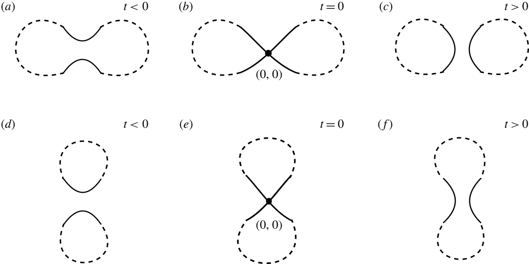
Illustration of the local changes in structure of the
 $Q=0$
contour curves during a pinching bifurcation. The solid lines illustrate the topology in a neighbourhood of the bifurcation point
 $(0,0)$
. The dashed lines in panels (a–c) show an example of a possible global structure for the case where the bifurcation results in the splitting of a single vortex into two; panels (d–f) illustrate the case when two vortices merge.

2.2
$H_{0}^{Q}$
indefinite: pinching bifurcation

Now we consider the case where
 $H_{0}^{Q}$
is indefinite. Then
 $H_{0}^{T}$
is also indefinite according to (2.7). It follows from (2.9c
) that in a neighbourhood of
 $(0,0)$
there exists a coordinate system
 $(\hat{x},{\hat{y}})$
where the zero contour curve of
 $Q$
is given by
 $$\begin{eqnarray}T(\hat{x},{\hat{y}})=\hat{x}^{2}-{\hat{y}}^{2}=t.\end{eqnarray}$$
For
 $t<0$
, the solution to this equation is a hyperbola with the
 ${\hat{y}}$
-axis as the principal axis; the zero contour curve of
 $Q$
is illustrated in figure 3(a). At
 $t=0$
the solution is the pair of straight lines given by
 ${\hat{y}}=\hat{x}$
and
 ${\hat{y}}=-\hat{x}$
which intersect at
 $(0,0)$
as shown in figure 3(b). If
 $t>0$
, the solution curve is a hyperbola with the
 $\hat{x}$
-axis as the principal axis; see figure 3(c) for a sketch of the zero contour curve of
 $Q$
. We will denote this kind of local change in structure as a pinching bifurcation of the
 $Q=0$
curve. The dashed lines in figure 3(a–c) illustrate how the pinching bifurcation can represent a vortex splitting into two. If the local level curves are connected globally up/down rather than left/right, the bifurcation represents the merging of two vortices, as shown in figure 3(d–f).
3 Bifurcations of
$Q=0$
curves at a no-slip boundary

In this section we consider a region of a fluid where a stationary no-slip boundary is present. We aim to describe the conditions under which the zero contours of
 $Q$
occur and how they erupt from that boundary. For simplicity we consider a boundary which coincides with the
 $x$
-axis. The theory can easily be generalized to any boundary described by a smooth curve. We choose the coordinate system such that fluid is present in the region where
 $y>0$
. The imposed no-slip conditions are then given by
 $$\begin{eqnarray}\left.\begin{array}{@{}c@{}}u(x,0,t)=\unicode[STIX]{x2202}_{y}\unicode[STIX]{x1D713}(x,0,t)=0,\\ v(x,0,t)=-\unicode[STIX]{x2202}_{x}\unicode[STIX]{x1D713}(x,0,t)=0,\end{array}\right\}\end{eqnarray}$$
where
 $\unicode[STIX]{x1D713}$
is the streamfunction. We notice that the velocities do not change along the boundary and all the higher-order derivatives in the
 $x$
-direction are therefore equal to zero,
 $$\begin{eqnarray}\unicode[STIX]{x2202}_{xx}\unicode[STIX]{x1D713}(x,0,t)=\unicode[STIX]{x2202}_{xxx}\unicode[STIX]{x1D713}(x,0,t)=\unicode[STIX]{x2202}_{xxxx}\unicode[STIX]{x1D713}(x,0,t)=\cdots =0\end{eqnarray}$$
and
 $$\begin{eqnarray}\unicode[STIX]{x2202}_{xy}\unicode[STIX]{x1D713}(x,0,t)=\unicode[STIX]{x2202}_{xxy}\unicode[STIX]{x1D713}(x,0,t)=\unicode[STIX]{x2202}_{xxxy}\unicode[STIX]{x1D713}(x,0,t)=\cdots =0.\end{eqnarray}$$
Since the
 $Q$
-value is defined as the determinant of the velocity gradient, it can be expressed in terms of the streamfunction as
 $$\begin{eqnarray}Q(x,y,t)=\unicode[STIX]{x2202}_{yy}\unicode[STIX]{x1D713}(x,y,t)\unicode[STIX]{x2202}_{xx}\unicode[STIX]{x1D713}(x,y,t)-\unicode[STIX]{x2202}_{xy}\unicode[STIX]{x1D713}(x,y,t)^{2}.\end{eqnarray}$$
From this expression it is clear that
 $Q(x,0,t)\equiv 0$
, implying that any point on a no-slip boundary will be part of the zero contour curve for
 $Q$
at any time
 $t$
. By differentiating (3.4) and exploiting that the higher-order derivatives in (3.2) and (3.3) are zero, we find that
 $$\begin{eqnarray}\unicode[STIX]{x2202}_{x}Q(x,0,t)=0\quad \text{and}\quad \unicode[STIX]{x2202}_{y}Q(x,0,t)=0,\end{eqnarray}$$
and
 $$\begin{eqnarray}\det (H^{Q}(x,0,t))=\unicode[STIX]{x2202}_{xx}Q(x,0,t)\unicode[STIX]{x2202}_{yy}Q(x,0,t)-\unicode[STIX]{x2202}_{xy}Q(x,0,t)^{2}=0.\end{eqnarray}$$
Thus, for any time
 $t$
, every point on a no-slip boundary is a critical point for
 $Q$
lying on the zero contour curve. Since the second derivative test is inconclusive according to (3.6), we need to perform a higher-order derivative test in order to locate possible bifurcation points. By Taylor’s theorem with integral remainder, we have for any fixed
 $x$
and any fixed
 $t$
,
 $$\begin{eqnarray}\displaystyle Q(x,y,t) & = & \displaystyle Q(x,0,t)+\unicode[STIX]{x2202}_{y}Q(x,0,t)y+\widetilde{Q}(x,y,t)y^{2}\nonumber\\ \displaystyle & = & \displaystyle \widetilde{Q}(x,y,t)y^{2},\end{eqnarray}$$
where
 $\widetilde{Q}$
is the continuous function defined as
 $$\begin{eqnarray}\widetilde{Q}(x,y,t)=\int _{0}^{1}\unicode[STIX]{x2202}_{yy}Q(x,y(1-s),t)s\,\text{d}s.\end{eqnarray}$$
From (3.7) we notice that
 $Q=0$
if
 $y=0$
or if
 $\widetilde{Q}=0$
. We can therefore determine the non-boundary part of the line where
 $Q=0$
by finding the zero contour curve of
 $\widetilde{Q}$
. Furthermore, we see that the sign of
 $Q$
is determined by the sign of
 $\widetilde{Q}$
for
 $y\neq 0$
. A region with positive
 $\widetilde{Q}$
-value is therefore classified as a vortex region. Hence, we will focus on the characteristics of
 $\widetilde{Q}$
instead of
 $Q$
. We are especially interested in finding the zeros of
 $\widetilde{Q}$
and it is therefore natural to ask under which physical conditions
 $\widetilde{Q}$
actually has zeros on the boundary. Since
 $$\begin{eqnarray}\unicode[STIX]{x1D714}(x,0,t)=-\unicode[STIX]{x1D6FB}^{2}\unicode[STIX]{x1D713}(x,0,t)=-\unicode[STIX]{x2202}_{yy}\unicode[STIX]{x1D713}(x,0,t),\end{eqnarray}$$
it follows from (3.8) and (3.4) that
 $$\begin{eqnarray}\displaystyle \widetilde{Q}(x,0,t) & = & \displaystyle {\textstyle \frac{1}{2}}\unicode[STIX]{x2202}_{yy}Q(x,0,t)\nonumber\\ \displaystyle & = & \displaystyle {\textstyle \frac{1}{2}}\unicode[STIX]{x2202}_{yy}\unicode[STIX]{x1D713}(x,0,t)\unicode[STIX]{x2202}_{xxyy}\unicode[STIX]{x1D713}(x,0,t)-\unicode[STIX]{x2202}_{xyy}\unicode[STIX]{x1D713}(x,0,t)^{2}\nonumber\\ \displaystyle & = & \displaystyle {\textstyle \frac{1}{2}}\unicode[STIX]{x1D714}(x,0,t)\unicode[STIX]{x2202}_{xx}\unicode[STIX]{x1D714}(x,0,t)-\unicode[STIX]{x2202}_{x}\unicode[STIX]{x1D714}(x,0,t)^{2}.\end{eqnarray}$$
This shows that
 $\widetilde{Q}$
on the boundary depends only on the vorticity and its derivatives along the boundary. Hence, bifurcations of
 $Q=0$
at the wall can be expressed in terms of the vorticity. There is no similar connection between
 $Q$
and
 $\unicode[STIX]{x1D714}$
away from the boundary. In the rest of this section we consider zero points of
 $\widetilde{Q}$
on the boundary and prove under which conditions these correspond to bifurcation points of the zero contour curves of
 $Q$
. For simplicity we choose a coordinate system such that zero points are located at
 $(x,y)=(0,0)$
at time
 $t=0$
and, as before, we use the subscript
 $0$
to denote any function evaluation at
 $(x,y,t)=(0,0,0)$
. First we consider a point on the no-slip boundary satisfying
 $$\begin{eqnarray}\displaystyle & \displaystyle \widetilde{Q}_{0}=0, & \displaystyle\end{eqnarray}$$
 $$\begin{eqnarray}\displaystyle & \displaystyle \unicode[STIX]{x2202}_{x}\widetilde{Q}_{0}\neq 0. & \displaystyle\end{eqnarray}$$
By the implicit function theorem it then follows that there exists a unique local function
 $X(y,t)=x$
satisfying
 $X(0,0)=0$
and
 $\widetilde{Q}(X(y,t),y,t)=0$
. The continuity of
 $X$
implies that, for any fixed
 $t$
sufficiently close to
 $t=0$
, there is a unique curve
 $x=X(y,t)$
, which intersects the boundary at
 $(x,y)=(X(0,t),0)$
. Since
 $\widetilde{Q}=0$
along this curve, it follows that for any
 $t$
sufficiently close to
 $t=0$
the zero contour curve of
 $\widetilde{Q}$
has a unique intersection with the boundary in a neighbourhood of
 $(x,y)=(0,0)$
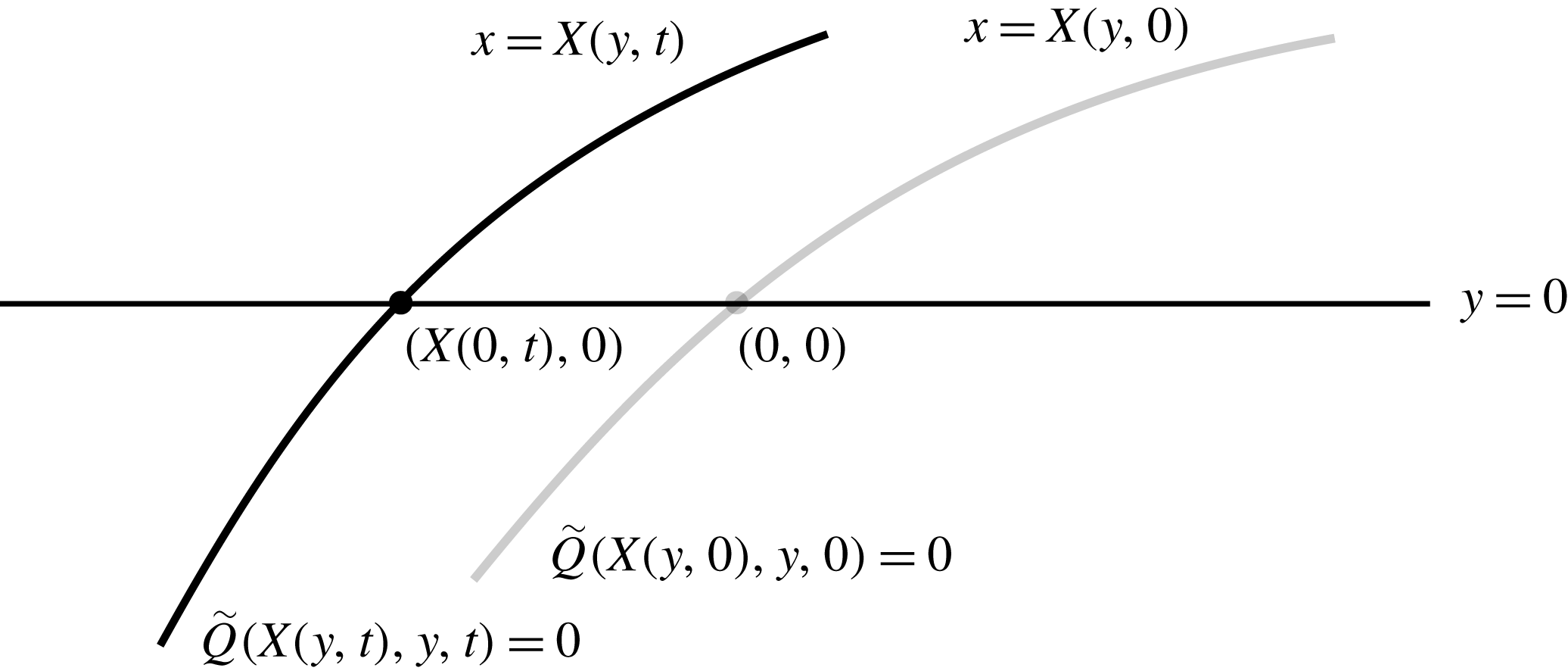
. Figure 4 illustrates how the zero contour of
 $\widetilde{Q}$
will maintain its intersection with the boundary for sufficiently small changes in time. To identify possible bifurcation points, we must therefore consider a boundary point
 $(x,y)=(0,0)$
satisfying that
 $$\begin{eqnarray}\widetilde{Q}_{0}=0,\quad \unicode[STIX]{x2202}_{x}\widetilde{Q}_{0}=0.\end{eqnarray}$$
To characterize bifurcations of codimension one, we assume that
 $\widetilde{Q}$
satisfies the simplest non-degeneracy conditions
 $$\begin{eqnarray}\unicode[STIX]{x2202}_{y}\widetilde{Q}_{0}\neq 0,\quad \unicode[STIX]{x2202}_{xx}\widetilde{Q}_{0}\neq 0\quad \text{and}\quad \unicode[STIX]{x2202}_{t}\widetilde{Q}_{0}\neq 0.\end{eqnarray}$$
At such a point it follows from the implicit function theorem that there exists a unique local function
 $Y(x,t)=y$
such that
 $Y_{0}=Y(0,0)=0$
and
 $\widetilde{Q}(x,Y(x,t),t)=0$
. This implies that for any fixed
 $t$
sufficiently close to
 $t=0$
, the zero contour curve of
 $\widetilde{Q}$
is given by the unique curve
 $y=Y(x,t)$
. By implicitly differentiating
 $\widetilde{Q}$
, we obtain that
 $$\begin{eqnarray}\unicode[STIX]{x2202}_{x}Y_{0}=-{\displaystyle \frac{\unicode[STIX]{x2202}_{x}\widetilde{Q}_{0}}{\unicode[STIX]{x2202}_{y}\widetilde{Q}_{0}}}=0\end{eqnarray}$$
and
 $$\begin{eqnarray}\unicode[STIX]{x2202}_{t}Y_{0}=-{\displaystyle \frac{\unicode[STIX]{x2202}_{t}\widetilde{Q}_{0}}{\unicode[STIX]{x2202}_{y}\widetilde{Q}_{0}}}\neq 0,\quad \unicode[STIX]{x2202}_{xx}Y_{0}=-{\displaystyle \frac{\unicode[STIX]{x2202}_{xx}\widetilde{Q}_{0}}{\unicode[STIX]{x2202}_{y}\widetilde{Q}_{0}}}\neq 0.\end{eqnarray}$$
Equations (3.15) and (3.16) show that the local behaviour of
 $Y$
around
 $(x,t)=(0,0)$
will now depend on the sign of the terms
 $\unicode[STIX]{x2202}_{y}\widetilde{Q}_{0}$
,
 $\unicode[STIX]{x2202}_{xx}\widetilde{Q}_{0}$
and
 $\unicode[STIX]{x2202}_{t}\widetilde{Q}_{0}$
. In the two sections below we consider the case where
 $\unicode[STIX]{x2202}_{xx}\widetilde{Q}_{0}$
and
 $\unicode[STIX]{x2202}_{y}\widetilde{Q}_{0}$
have the same sign and the case where their signs are different. As we will see, these cases result in two different types of bifurcations.
Illustration of how a small change in time affects the topological structure of the contour curve,
 $\widetilde{Q}=0$
, close to a non-critical boundary point
 $(0,0)$
. Since the topological structure is unchanged,
 $(0,0)$
is not a bifurcation point.

3.1 Wall-punching bifurcation
We first consider the case where
 $$\begin{eqnarray}\text{sign}(\unicode[STIX]{x2202}_{xx}\widetilde{Q}_{0})=\text{sign}(\unicode[STIX]{x2202}_{y}\widetilde{Q}_{0}).\end{eqnarray}$$
Furthermore, we assume that
 $\unicode[STIX]{x2202}_{t}\widetilde{Q}_{0}$
has the opposite sign to
 $\unicode[STIX]{x2202}_{xx}\widetilde{Q}_{0}$
and
 $\unicode[STIX]{x2202}_{y}\widetilde{Q}_{0}$
. Then
 $\unicode[STIX]{x2202}_{xx}Y_{0}<0$
and there is an interval around
 $x=0$
where
 $Y(x,0)$
is a strictly concave function with maximum value in
 $x=0$
. The corresponding zero contour curve of
 $Q$
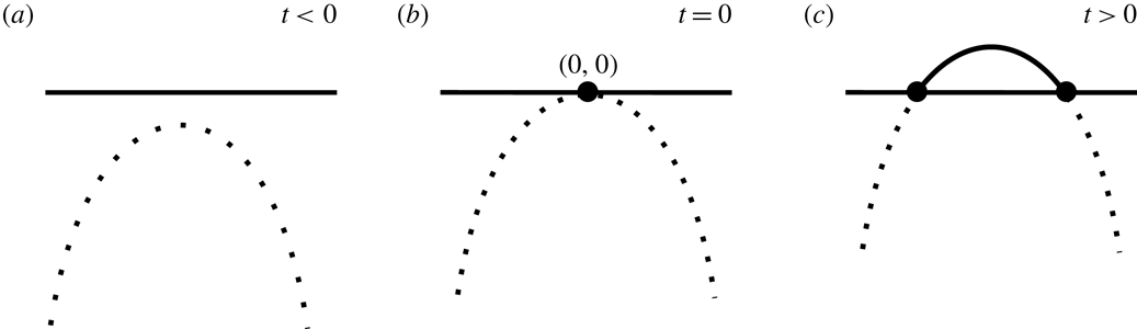
is illustrated in figure 5(b). To investigate what happens to the curve for
 $t\neq 0$
, we apply the implicit function theorem yet again. By the conditions in (3.15) and (3.16) there exists a unique function
 $T(x)=t$
, such that
 $T_{0}=T(0)=0$
and
 $Y(x,T(x))=0$
for any
 $x$
sufficiently close to
 $0$
. By implicit differentiation of
 $Y$
, we obtain that
 $$\begin{eqnarray}\unicode[STIX]{x2202}_{x}T_{0}=-{\displaystyle \frac{\unicode[STIX]{x2202}_{x}Y_{0}}{\unicode[STIX]{x2202}_{t}Y_{0}}}=0\quad \text{and}\quad \unicode[STIX]{x2202}_{xx}T_{0}=-{\displaystyle \frac{\unicode[STIX]{x2202}_{xx}Y_{0}}{\unicode[STIX]{x2202}_{t}Y_{0}}}>0.\end{eqnarray}$$
Illustration of the local changes in structure under a wall-punching bifurcation. The figure illustrates the forward version where
 $\text{sign}(\unicode[STIX]{x2202}_{t}\widetilde{Q}_{0})\neq \text{sign}(\unicode[STIX]{x2202}_{y}\widetilde{Q}_{0})$
. The solid lines are the visible zero contour curves of
 $Q$
, while the dotted lines are outside the region containing the fluid.

These conditions imply that
 $T$
is a strictly convex function with minimum value at
 $x=0$
. Hence, there are no solutions to the equation
 $T(x)=t$
if
 $t<0$
and two solutions if
 $t>0$
. Since
 $T$
is a unique function we conclude that, in a neighbourhood of
 $x=0$
,
 $Y$
has no zero points for
 $t<0$
and two zero points for
 $t>0$
. These two scenarios are illustrated in figure 5(a,c). The structural change we observe corresponds to the zero contour of
 $\widetilde{Q}$
breaking through the boundary at the bifurcation point
 $(x,y,t)=(0,0,0)$
. We denote this kind of structural change as a wall-punching bifurcation. From a physical point of view, a wall-punching bifurcation corresponds to a vortex being created attached to the wall. If we instead consider the situation where
 $$\begin{eqnarray}\text{sign}(\unicode[STIX]{x2202}_{xx}\widetilde{Q}_{0})=\text{sign}(\unicode[STIX]{x2202}_{y}\widetilde{Q}_{0})=\text{sign}(\unicode[STIX]{x2202}_{t}\widetilde{Q}_{0}),\end{eqnarray}$$
an entirely similar argument shows that the wall-punching bifurcation will occur backwards and describes the case where a vortex disappears through the boundary.
3.2 Wall-pinching bifurcation
So far we have only considered the case where (3.17) is satisfied. If we instead consider the case where
 $$\begin{eqnarray}\text{sign}(\unicode[STIX]{x2202}_{xx}\widetilde{Q}_{0})\neq \text{sign}(\unicode[STIX]{x2202}_{y}\widetilde{Q}_{0}),\end{eqnarray}$$
then
 $Y(x,0)$
is strictly convex. From arguments similar to the above, it is easy to prove that, if
 $\text{sign}(\unicode[STIX]{x2202}_{t}\widetilde{Q}_{0})\neq \text{sign}(\unicode[STIX]{x2202}_{y}\widetilde{Q}_{0})$
, the zero contour curve will intersect the wall in two points for
 $t<0$
and will pinch off the wall for
 $t>0$
, as shown in figure 6. For
 $\text{sign}(\unicode[STIX]{x2202}_{t}\widetilde{Q}_{0})=\text{sign}(\unicode[STIX]{x2202}_{y}\widetilde{Q}_{0})$
the reverse change occurs. We denote this type of structural change as a wall-pinching bifurcation. From a physical point of view, a wall-pinching bifurcation corresponds to a vortex detaching from or attaching to the wall.
4 Degeneracies and codimension-two bifurcations
In the previous sections we have provided a complete analysis of all possible bifurcations of codimension one, i.e. bifurcations that occur at a specific value of the bifurcation parameter, which we chose to be time. Each of the four bifurcations occurs under a specific set of degeneracy conditions (equalities) and non-degeneracy conditions (inequalities). The non-degeneracy conditions may, of course, turn out to be violated. To determine the conditions under which this occurs, we turn the relevant non-degeneracy condition into an additional degeneracy condition by insisting on its violation. This imposition then provides an additional equation that allows us to determine particular values of some additional parameter (e.g. the Reynolds number) at which this degeneracy occurs. Such points are known as codimension-two points because they require two parameters (here time and the Reynolds number) to take on particular values for the degenerate behaviour to occur.
For the bifurcations away from boundaries, the non-degeneracy conditions (2.4) and (2.5) require that the Hessian of
 $Q$
is non-singular and that
 $\unicode[STIX]{x2202}_{t}Q_{0}\neq 0$
, respectively. In appendix A we analyse the case where the second non-degeneracy condition is broken, such that the degeneracy conditions are
 $$\begin{eqnarray}Q_{0}=\unicode[STIX]{x2202}_{x}Q_{0}=\unicode[STIX]{x2202}_{y}Q_{0}=\unicode[STIX]{x2202}_{t}Q_{0}=0.\end{eqnarray}$$
The first non-degeneracy condition is kept, and other conditions will be imposed to allow the use of the implicit function theorem. We choose this case as it appears in the application we study below. The analysis shows that close to the codimension-two point
 $(t_{0},Re_{0})$
there is a bifurcation curve in the
 $(t,Re)$
parameter plane given by
 $$\begin{eqnarray}Re=Re_{0}+C(t-t_{0})^{2}+O(t^{3}),\end{eqnarray}$$
where
 $C$
is a constant. If
 $C>0$
, and
 $Re$
is slightly larger than
 $Re_{0}$
, there are punching bifurcations when the bifurcation curve is crossed, i.e. when
 $t=t_{0}\pm \sqrt{(Re-Re_{0})}/\sqrt{C}+O(Re-Re_{0})$
. The first crossing is the creation of a vortex by a punching bifurcation; the latter is the destruction of a vortex by a backward punching bifurcation. If
 $Re<Re_{0}$
, the bifurcation curve is not crossed, and no bifurcations occur near
 $t_{0}$
.
Illustration of the local changes in structure under a wall-pinching bifurcation. The figure illustrates the forward version where
 $\text{sign}(\unicode[STIX]{x2202}_{t}\widetilde{Q}_{0})\neq \text{sign}(\unicode[STIX]{x2202}_{y}\widetilde{Q}_{0})$
. The solid lines are the visible zero contour curves of
 $Q$
, while the dotted line is outside the region containing the fluid.

5 Application to boundary layer eruption
5.1 Problem set-up
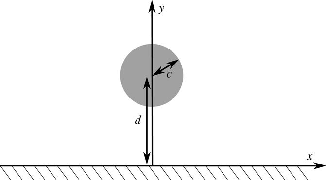
As a case study we consider a vortex convected close to a no-slip wall. Such a vortex induces a viscous response from the boundary layer close to the wall. The vorticity in the boundary layer may organize itself into new vortex structures that erupt from the surface. This phenomenon is known as boundary layer eruption (Kudela & Malecha Reference Kudela and Malecha2009), unsteady separation (Williams Reference Williams1977) or bursting (Robinson Reference Robinson1991). To give a mathematical formulation of the phenomenon, we choose a coordinate system fixed to the no-slip wall as shown in figure 7. The initial configuration is a Gaussian vortex with characteristic length
 $c$
and negative vorticity
 $-\unicode[STIX]{x1D714}_{0}$
at the vortex centre. The Gaussian vortex is placed at distance
 $d$
from the wall and an image vortex with opposite vorticity is placed below the wall. Owing to symmetry the velocity field satisfies the non-penetration condition on the wall. A boundary layer is created when, at
 $t=0$
, we impose the no-slip condition. We non-dimensionalize our problem by choosing the reference length
 $L=d$
and the reference velocity
 $U={\textstyle \frac{1}{2}}\unicode[STIX]{x1D714}_{0}c$
. For our choice of non-dimensionalization, the Reynolds number is given by
 $$\begin{eqnarray}Re=\frac{LU}{\unicode[STIX]{x1D708}}=\frac{\unicode[STIX]{x1D714}_{0}dc}{2\unicode[STIX]{x1D708}},\end{eqnarray}$$
where
 $\unicode[STIX]{x1D708}$
is the kinematic viscosity of the fluid. We specify the initial vortex by the dimensionless parameter
 $a$
that represents the ratio between the size of the initial vortex and the distance to the wall, i.e.
 $a=c/d$
. In order to be consistent with earlier studies by Kudela & Malecha (Reference Kudela and Malecha2009) and Andersen (Reference Andersen2013), we have chosen the parameter value
 $a=0.3$
. We note that our choice of non-dimensionalization gives us a Reynolds number that is a scaled version of the Reynolds number,
 $\widehat{Re}$
, used by Kudela & Malecha (Reference Kudela and Malecha2009) and Andersen (Reference Andersen2013). The scaling is
 $Re={\textstyle \frac{1}{2}}\unicode[STIX]{x1D6FA}_{0}a\widehat{Re}$
, with
 $\unicode[STIX]{x1D6FA}_{0}=1.25$
.
Initial configuration of the boundary layer eruption problem. A Gaussian vortex is placed at a distance
 $d$
from the no-slip wall; and
 $c$
is the characteristic length for the Gaussian distribution.

5.2 Numerical method
We performed our numerical simulations using the open-source finite element library oomph-lib (Heil & Hazel Reference Heil and Hazel2006), discretizing the Navier–Stokes equations with LBB-stable quadrilateral Taylor–Hood (Q2Q1) elements and employing a BDF2 scheme for the time integration. The vortex–wall interaction results in a net advection of the initial vortex in the negative
 $x$
-direction. To avoid the need for a large computational domain, we performed the computations in a domain that moves steadily with the initial velocity of the advecting vortex. This allowed us to restrict the computational domain to the region
 $x\in [-3.63,3.63]$
and
 $y\in [0,5.13]$
. The computations were started from an initial velocity field given by the Gaussian vortex and its mirror image below the
 $y$
-axis. During a short initial period we only enforced the non-penetration condition and then imposed the no-slip condition on the wall to initiate the formation of the boundary layer. On the remaining boundaries we imposed the velocity associated with the initial vortex (corrected for the moving frame of reference). To resolve the boundary layer, we decomposed the mesh into two regions: within a thin layer close to the wall we decreased the distance between the mesh points exponentially towards the wall; a uniform mesh spacing was used in the rest of the domain. The
 $Q$
-field and its derivatives were computed using the oomph-lib (Heil & Hazel Reference Heil and Hazel2006) derivative recovery techniques to obtain smooth approximations of the required derivatives (see Heil et al. (Reference Heil, Rosso, Hazel and Brøns2017) for details). To confirm that our results were fully converged, we recomputed selected cases on refined meshes and with smaller time steps.
5.3 Numerical results
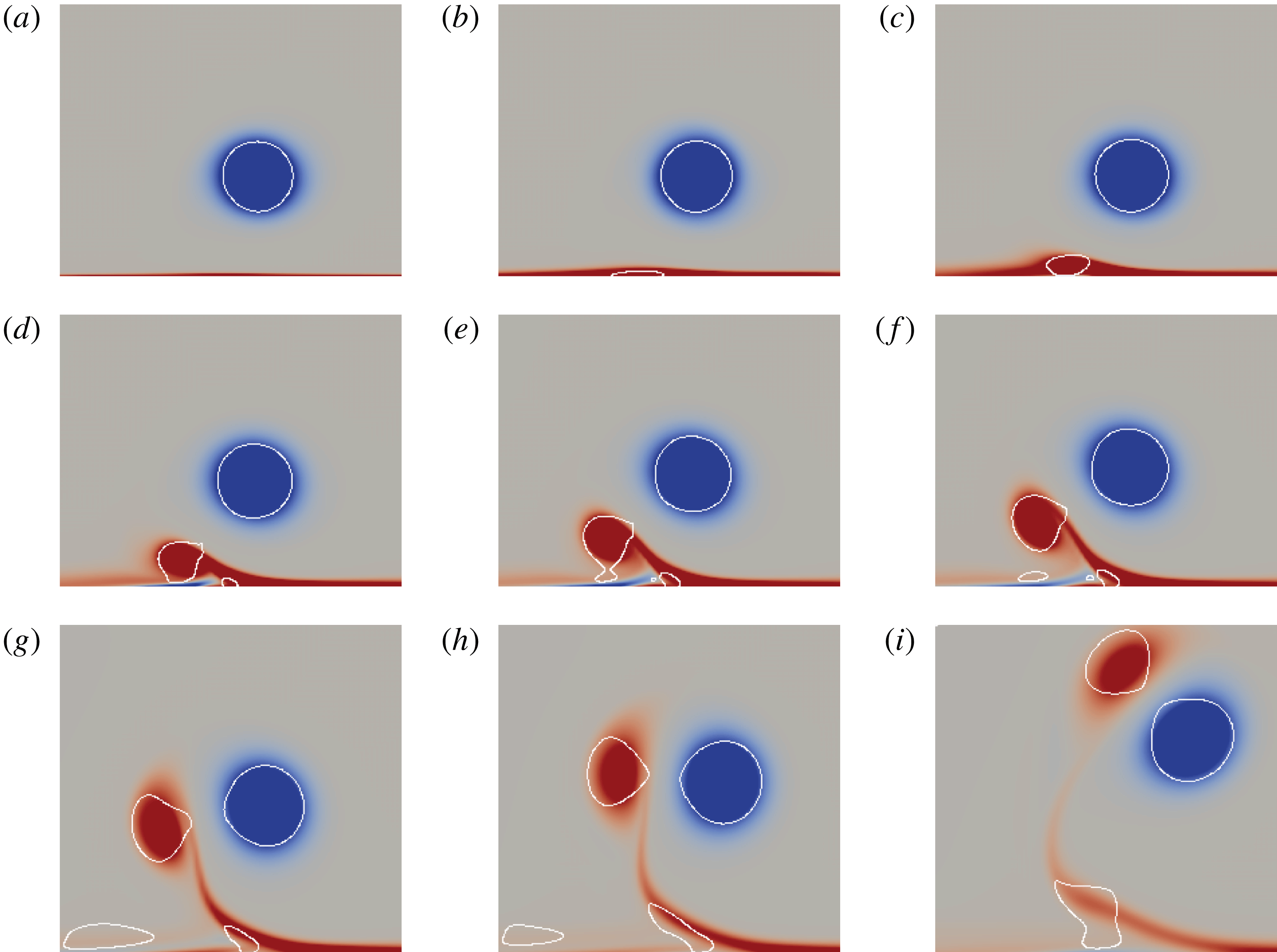
Numerical results for
 $Re=2063$
at the following time steps: (a)
 $t=11$
, (b)
 $t=48$
, (c)
 $t=117$
, (d)
 $t=197$
, (e)
 $t=256$
, (f)
 $t=293$
, (g)
 $t=395$
, (h)
 $t=464$
and (i)
 $t=597$
. Each panel shows a zoom in on the region close to the initial vortex, where
 $x\in [-2,1.5]$
. The vorticity contours with values from
 $-0.3$
to
 $0.3$
are coloured in blue and red. Regions with positive
 $Q$
-value are encircled by white lines, which correspond to the zero contour curves of
 $Q$
.

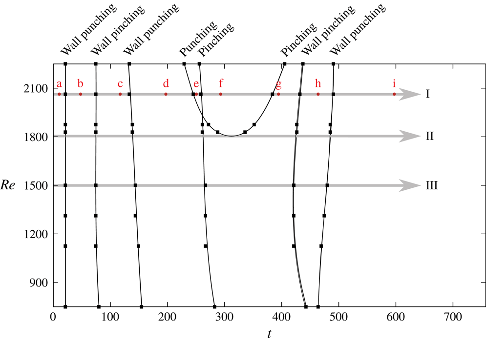
Bifurcation diagram of the eruption process. The red dots marked with a letter correspond to the plots shown in figure 8. The black squares, connected by solid lines, mark the bifurcation points observed in the simulations. The grey arrows indicate in which sequence the bifurcations are encountered in a flow with a given Reynolds number.

We simulated the early stages of boundary layer eruption at moderate Reynolds numbers in the range between
 $Re=750$
and
 $Re=2250$
. Figure 8 shows snapshots from a simulation with
 $Re=2063$
. The zero contour curves of
 $Q$
are drawn on top of the vorticity field to provide a basis for comparison. Each of the nine panels represents a topological vortex structure observed in the simulation. In figure 8(a) the initial vortex is the only region with positive
 $Q$
-value. At this early stage the shape of the vortex is very close to a perfect circle. This is consistent with a result by Elsas & Moriconi (Reference Elsas and Moriconi2017), who showed that a Gaussian vortex will have a positive
 $Q$
-value in a circular region with radius
 $r\approx c/0.89$
. For a Gaussian vortex, the radius grows like
 $\sqrt{t}$
, which is identical to the initial growth rate we found for a vortex generated in a punching bifurcation (see § 2).
The overall changes in the vortex structure in figure 8 can be described as eight separate bifurcations of the zero contour curves. In the time span between panels (a) and (b) we see an example of a wall-punching bifurcation that causes a new vortex to form in the boundary layer. In figure 8(c) this new vortex has detached from the wall as the result of a wall-pinching bifurcation. After another wall-punching bifurcation, a second vortex is formed in the boundary layer, as shown in panel (d). In the time span between figure 8(d) and (e) a punching bifurcation takes place and a small vortex develops in the part of the boundary layer with negative vorticity. Between figure 8(e) and (f) we observe a pinching bifurcation where the largest vortex splits into two vortices. In the last three steps, two vortices disappear as a result of two punching bifurcations and the vortex at the wall detaches via a wall-pinching bifurcation. The structure shown in figure 8(i) then persists for the rest of the simulated time span, implying that, at this Reynolds number, two long-lasting vortices emerge from the boundary layer. In the course of their formation, several transitional vortex structures appear and our theory is able give a complete description of the topological changes in the flow field as a series of bifurcations in the
 $Q$
-contours.
To illustrate how the formation of the vortices depends on the Reynolds number, we construct a bifurcation diagram of the eruption process (see figure 9). The black squares in the diagram mark the times at which the various bifurcations are observed in the simulations. The thick grey lines trace out the temporal evolution at fixed Reynolds numbers. Line I corresponds to the case just discussed (
 $Re=2063$
), with the circular symbols indicating the times at which the snapshots in figure 8 were taken. We have connected bifurcation points of the same type by solid lines to indicate that we expect a similar evolution in between the simulations presented in the diagram.
However, the U-shaped curve tracing out the punching bifurcation is an exception. The bifurcation points on this curve do not satisfy the same non-degeneracy conditions. The squares on the left branch of the curve mark a forward punching bifurcation where
 $\unicode[STIX]{x2202}_{t}Q_{0}>0$
and the squares on the right branch mark a backward punching bifurcation where
 $\unicode[STIX]{x2202}_{t}Q_{0}<0$
. This change of sign of
 $\unicode[STIX]{x2202}_{t}Q$
indicates the existence of a codimension-two point
 $(t_{0},Re_{0})$
where
 $\unicode[STIX]{x2202}_{t}Q_{0}=0$
. According to (4.2) the bifurcation curve close to such a point is approximately parabolic. Making a least-squares fit to a parabola of the four nearest data points yields the expression
 $$\begin{eqnarray}Re=1817+0.0458(t-312)^{2},\end{eqnarray}$$
from which we get the estimate of the codimension-two point
 $(t_{0},Re_{0})=(312,1817)$
.
It is important to notice that we have estimated the codimension-two point without actually solving the equations (4.1) that characterize it. The simulation results are interpreted within the framework of the bifurcation theory we have developed, and are consistent with the codimension-two case we have analysed.
In summary, over the range of Reynolds numbers considered in the bifurcation diagram, the final outcome of the evolution is the same: two vortices emerge from the erupting boundary layer and the time at which the various bifurcations occur only changes very little with
 $Re$
. The only exception is the codimension-two phenomenon at
 $Re=1817$
(line II in figure 9) that separates the parameter space into two regions with distinct evolution of the topology of the vortices. For
 $Re>1817$
, exemplified by line I in figure 9, a small vortex appears and disappears again close to the wall. As
 $Re$
is decreased, its lifetime diminishes and for
 $Re<1817$
, exemplified by line III, the vortex does not appear at all.
6 Discussion
Using the
 $Q$
-criterion we have formulated a theory describing the evolution of vortices in two-dimensional incompressible flow. The theory is complete in the sense that it identifies all possible codimension-one bifurcations of the
 $Q=0$
contour curves. Our theory provides a systematic approach to describing topological changes associated with the creation/destruction and the merging/splitting of vortices. The possible types of bifurcations serve as templates that facilitate the construction of a bifurcation diagram. Despite the fact that the mathematical analysis is technical the results are easy to apply. A vortex bifurcation event occurs when
 $Q=\unicode[STIX]{x2202}_{x}Q=\unicode[STIX]{x2202}_{y}Q=0$
and the type of event depends only on higher-order derivatives of
 $Q$
. At a no-slip wall
 $y=0$
the corresponding conditions are
 $\widetilde{Q}=\unicode[STIX]{x2202}_{x}\widetilde{Q}=0$
, where
 $\widetilde{Q}=Q/y^{2}$
. The degeneracy and non-degeneracy conditions required to locate and identify each type of bifurcation can therefore be computed directly from derivatives of the velocity field.
Numerical simulations of boundary layer eruption at moderate Reynolds numbers showed that all four types of codimension-one bifurcations occur in that flow. We also observed the occurrence of a codimension-two bifurcation at
 $Re=1817$
. It arises via the coalescence of two codimension-one bifurcations that are associated with the creation/destruction of a particular vortex. This vortex does not develop for smaller Reynolds numbers but has an increasing lifespan as the Reynolds number increases above 1817. We were able to infer the existence of the codimension-two point and showed how to determine its location using only knowledge about the
 $Q=0$
contour, i.e. without requiring derivatives of
 $Q$
. This may be the most important message of the present paper: bifurcation theory provides a list of possible vortex bifurcation events. Observations of changes in the topology of the
 $Q=0$
contour in specific computational or experimental data can be matched with a bifurcation event which is mathematically well understood, leading to an interpretation of the data which rests on a solid theoretical basis.
If the Reynolds number is increased beyond the range considered in our case study, additional codimension-two points are likely to arise. If that is the case, it would be useful to give a complete analysis of all codimension-two cases, as outlined in § 4. Another important extension would be to generalize the theory to three-dimensional flows. In this case the zero contours of
 $Q$
are surfaces in three dimensions. Much of our analysis will carry over, using the three-dimensional version of the Morse lemma. In particular, a vortex bifurcation event will occur when
 $Q=\unicode[STIX]{x2202}_{x}Q=\unicode[STIX]{x2202}_{y}Q=\unicode[STIX]{x2202}_{z}Q=0$
.
Finally, we note that the bifurcations in the topology of the
 $Q=0$
curves are much simpler than those found by Balci et al. (Reference Balci, Andersen, Thompson and Brøns2015) in the topology of the instantaneous streamlines. When studying the boundary layer eruption process using the latter approach, a bifurcation diagram of codimension three was needed to describe the eruption process completely. We therefore believe that the concepts proposed in the present paper will be helpful for interpreting and classifying vortex interactions in a large range of flows obtained either numerically or experimentally.
Appendix A. Analysis of a particular codimension-two bifurcation
In this appendix we analyse the codimension-two bifurcation that arises when a forward and a reverse punching bifurcation coalesce at a particular value of the Reynolds number, leading to the violation of the non-degeneracy condition
 $\unicode[STIX]{x2202}_{t}Q_{0}\neq 0$
.
To identify the time and Reynolds number at which this scenario arises, we introduce a second parameter,
 $r$
, representing the deviation of the Reynolds number from the value at which the codimension-two bifurcation occurs. We then choose a coordinate system such that a bifurcation point is located at
 $(x,y,t,r)=(0,0,0,0)$
and, as before, we use subscript
 $0$
to denote evaluation at the bifurcation point. We consider a bifurcation point that is characterized by the following set of degeneracy conditions:
 $$\begin{eqnarray}Q_{0}=0,\quad \unicode[STIX]{x2202}_{x}Q_{0}=0,\quad \unicode[STIX]{x2202}_{y}Q_{0}=0,\quad \unicode[STIX]{x2202}_{t}Q_{0}=0.\end{eqnarray}$$
The first three of these are simply the conditions (2.3) required for the occurrence of a punching bifurcation. The final condition ensures that the first of the two non-degeneracy conditions, equation (2.5), is violated.
We now augment these conditions by the following non-degeneracy conditions:
 $$\begin{eqnarray}\unicode[STIX]{x2202}_{r}Q_{0}>0,\quad \unicode[STIX]{x2202}_{tt}Q_{0}<0\end{eqnarray}$$
and
 $$\begin{eqnarray}H_{0}^{Q}=\left(\begin{array}{@{}ccc@{}}\unicode[STIX]{x2202}_{xx}Q_{0} & \unicode[STIX]{x2202}_{xy}Q_{0} & \unicode[STIX]{x2202}_{xt}Q_{0}\\ \unicode[STIX]{x2202}_{xy}Q_{0} & \unicode[STIX]{x2202}_{yy}Q_{0} & \unicode[STIX]{x2202}_{yt}Q_{0}\\ \unicode[STIX]{x2202}_{xt}Q_{0} & \unicode[STIX]{x2202}_{yt}Q_{0} & \unicode[STIX]{x2202}_{tt}Q_{0}\\ \end{array}\right)\text{ is negative definite}.\end{eqnarray}$$
Using these conditions we will now show that there is a bifurcation curve
 $r(t)=Ct^{2}+O(t^{3})$
, where
 $C$
is a positive constant, which separates the
 $(t,r)$
parameter space into two regions, one where a vortex is present and one where there is none. Thus, for a small fixed
 $r>0$
, a vortex is created in a punching bifurcation at
 $t\approx -\sqrt{r/C}$
. The vortex disappears again in a reverse punching bifurcation at
 $t\approx \sqrt{r/C}$
– exactly as seen in figure 9.
We start by observing that, since
 $Q_{0}=0$
and
 $\unicode[STIX]{x2202}_{r}Q_{0}\neq 0$
, it follows from the implicit function theorem that there exists a unique local function
 $R(x,y,t)=r$
satisfying that
 $R_{0}=0$
and
 $Q(x,y,t,R(x,y,t))=0$
. By implicit differentiation of
 $Q$
, we obtain that
 $$\begin{eqnarray}\unicode[STIX]{x2202}_{x}R_{0}=-{\displaystyle \frac{\unicode[STIX]{x2202}_{x}Q_{0}}{\unicode[STIX]{x2202}_{r}Q_{0}}}=0,\quad \unicode[STIX]{x2202}_{y}R_{0}=-{\displaystyle \frac{\unicode[STIX]{x2202}_{y}Q_{0}}{\unicode[STIX]{x2202}_{r}Q_{0}}}=0,\quad \unicode[STIX]{x2202}_{t}R_{0}=-{\displaystyle \frac{\unicode[STIX]{x2202}_{t}Q_{0}}{\unicode[STIX]{x2202}_{r}Q_{0}}}=0,\end{eqnarray}$$
and the Hessian
 $$\begin{eqnarray}H_{0}^{R}=\left(\begin{array}{@{}ccc@{}}\unicode[STIX]{x2202}_{xx}R_{0} & \unicode[STIX]{x2202}_{xy}R_{0} & \unicode[STIX]{x2202}_{xt}R_{0}\\ \unicode[STIX]{x2202}_{xy}R_{0} & \unicode[STIX]{x2202}_{yy}R_{0} & \unicode[STIX]{x2202}_{yt}R_{0}\\ \unicode[STIX]{x2202}_{xt}R_{0} & \unicode[STIX]{x2202}_{yt}R_{0} & \unicode[STIX]{x2202}_{tt}R_{0}\\ \end{array}\right)=-{\displaystyle \frac{1}{\unicode[STIX]{x2202}_{r}Q_{0}}}H_{0}^{Q}.\end{eqnarray}$$
Since
 $\unicode[STIX]{x2202}_{r}Q_{0}>0$
and
 $H_{0}^{Q}$
is negative definite, it follows from (A 5) that
 $H_{0}^{R}$
is positive definite. Hence, it follows by Sylvester’s criterion that the upper left
 $2\times 2$
corner of
 $H_{0}^{R}$
is also positive definite. The conditions in (A 4) and (A 5), therefore, allow us to apply the implicit function theorem, this time on the gradient of
 $R$
. Hence, we conclude that there exist unique local functions
 $X(t)=x$
and
 $Y(t)=y$
satisfying that
 $X_{0}=0$
,
 $Y_{0}=0$
and
 $$\begin{eqnarray}\left(\begin{array}{@{}c@{}}\unicode[STIX]{x2202}_{x}R(X(t),Y(t),t)\\ \unicode[STIX]{x2202}_{y}R(X(t),Y(t),t)\end{array}\right)=\mathbf{0}.\end{eqnarray}$$
The generalized version of the Morse lemma depending on parameters (Hörmander Reference Hörmander2007) implies that in a neighbourhood of the critical point
 $(x,y)=(0,0)$
there exists a (possibly nonlinear) coordinate change,
 $\hat{x}=\hat{x}(x,y)$
,
 ${\hat{y}}={\hat{y}}(x,y)$
, such that
 $$\begin{eqnarray}\hat{x}(0,0)=0,\quad {\hat{y}}(0,0)=0\end{eqnarray}$$
and
 $$\begin{eqnarray}R(\hat{x},{\hat{y}},t)=R(X(t),Y(t),t)+\hat{x}^{2}+{\hat{y}}^{2}.\end{eqnarray}$$
In the new coordinate system the zero contour curve of
 $Q$
is therefore given by the equation
 $$\begin{eqnarray}\hat{x}^{2}+{\hat{y}}^{2}=r-R(X(t),Y(t),t).\end{eqnarray}$$
The right-hand side of (A 9) determines whether or not there exist any points, sufficiently close to
 $(\hat{x},{\hat{y}})=(0,0)$
, which are part of the zero contour curve of
 $Q$
. The curve
 $r(t)=R(X(t),Y(t),t)$
therefore separates the parameter space into two regions: one where a vortex region is present, and one where it is not. We find
 $$\begin{eqnarray}\displaystyle \left.\begin{array}{@{}c@{}}r^{\prime }(t)=\unicode[STIX]{x1D735}R(X(t),X(t),t)\boldsymbol{\cdot }\boldsymbol{x}^{\prime }(t),\\ r^{\prime \prime }(t)=\boldsymbol{x}^{\prime }(t)^{\text{T}}\boldsymbol{\cdot }H^{R}(X(t),Y(t),t)\boldsymbol{\cdot }\boldsymbol{x}^{\prime }(t)+\unicode[STIX]{x1D735}R(X(t),Y(t),t)\boldsymbol{\cdot }\boldsymbol{x}^{\prime \prime }(t),\end{array}\right\} & & \displaystyle\end{eqnarray}$$
where
 $$\begin{eqnarray}\boldsymbol{x}(t)=\left(\begin{array}{@{}c@{}}X(t)\\ Y(t)\\ t\end{array}\right)\!.\end{eqnarray}$$
By (A 4) and (A 5) it follows that
 $\unicode[STIX]{x1D735}R_{0}=\mathbf{0}$
and
 $H_{0}^{R}$
is positive definite. Since
 $\boldsymbol{x}^{\prime }(t)$
is non-zero for all
 $t$
, it follows that
 $$\begin{eqnarray}\displaystyle \left.\begin{array}{@{}c@{}}r^{\prime }(0)=0,\\ r^{\prime \prime }(0)=\boldsymbol{x}^{\prime }(0)^{\text{T}}\boldsymbol{\cdot }H_{0}^{R}\boldsymbol{\cdot }\boldsymbol{x}^{\prime }(0)>0.\end{array}\right\} & & \displaystyle\end{eqnarray}$$
By Taylor expansion of
 $r$
at
 $t=0$
we get the desired result
 $$\begin{eqnarray}r(t)=Ct^{2}+O(t^{3}),\end{eqnarray}$$
where
 $C={\textstyle \frac{1}{2}}\boldsymbol{x}^{\prime }(0)^{\text{T}}\boldsymbol{\cdot }H_{0}^{R}\boldsymbol{\cdot }\boldsymbol{x}^{\prime }(0)>0$
.
We have proved that in a neighbourhood of a codimension-two point the curve
 $r(t)=Ct^{2}+O(t^{3})$
is a bifurcation curve. The non-degeneracy condition
 $\unicode[STIX]{x2202}_{tt}Q_{0}<0$
and the continuity of
 $\unicode[STIX]{x2202}_{t}Q$
imply that
 $\unicode[STIX]{x2202}_{t}Q$
is positive on the left branch of the curve and negative on the right branch. The only point on the curve satisfying the conditions in (A 1) is therefore the bifurcation point at
 $(x,y,t,r)=(0,0,0,0)$
and all other points on the curve must be bifurcation points with codimension one.
By Sylvester’s criterion the upper left
 $2\times 2$
corner of
 $H_{0}^{Q}$
is negative definite when
 $H_{0}^{Q}$
is negative definite. By continuity, it therefore follows for all other points on the bifurcation curve that
 $$\begin{eqnarray}Q=0,\quad \unicode[STIX]{x2202}_{x}Q=0,\quad \unicode[STIX]{x2202}_{y}Q=0,\quad \unicode[STIX]{x2202}_{t}Q\neq 0\end{eqnarray}$$
and
 $$\begin{eqnarray}\left(\begin{array}{@{}cc@{}}\unicode[STIX]{x2202}_{xx}Q & \unicode[STIX]{x2202}_{xy}Q\\ \unicode[STIX]{x2202}_{xy}Q & \unicode[STIX]{x2202}_{yy}Q\end{array}\right)\text{is negative definite}.\end{eqnarray}$$
These conditions are identical to the conditions in § 2, implying that a punching bifurcation occurs forward on the left-hand side of the bifurcation curve, where
 $\unicode[STIX]{x2202}_{t}Q$
is positive. In contrast,
 $\unicode[STIX]{x2202}_{t}Q$
is negative on the right-hand side of the curve, and here a punching bifurcation occurs backward at any point. This is completely consistent with the behaviour observed in figure 9.