

1. Introduction
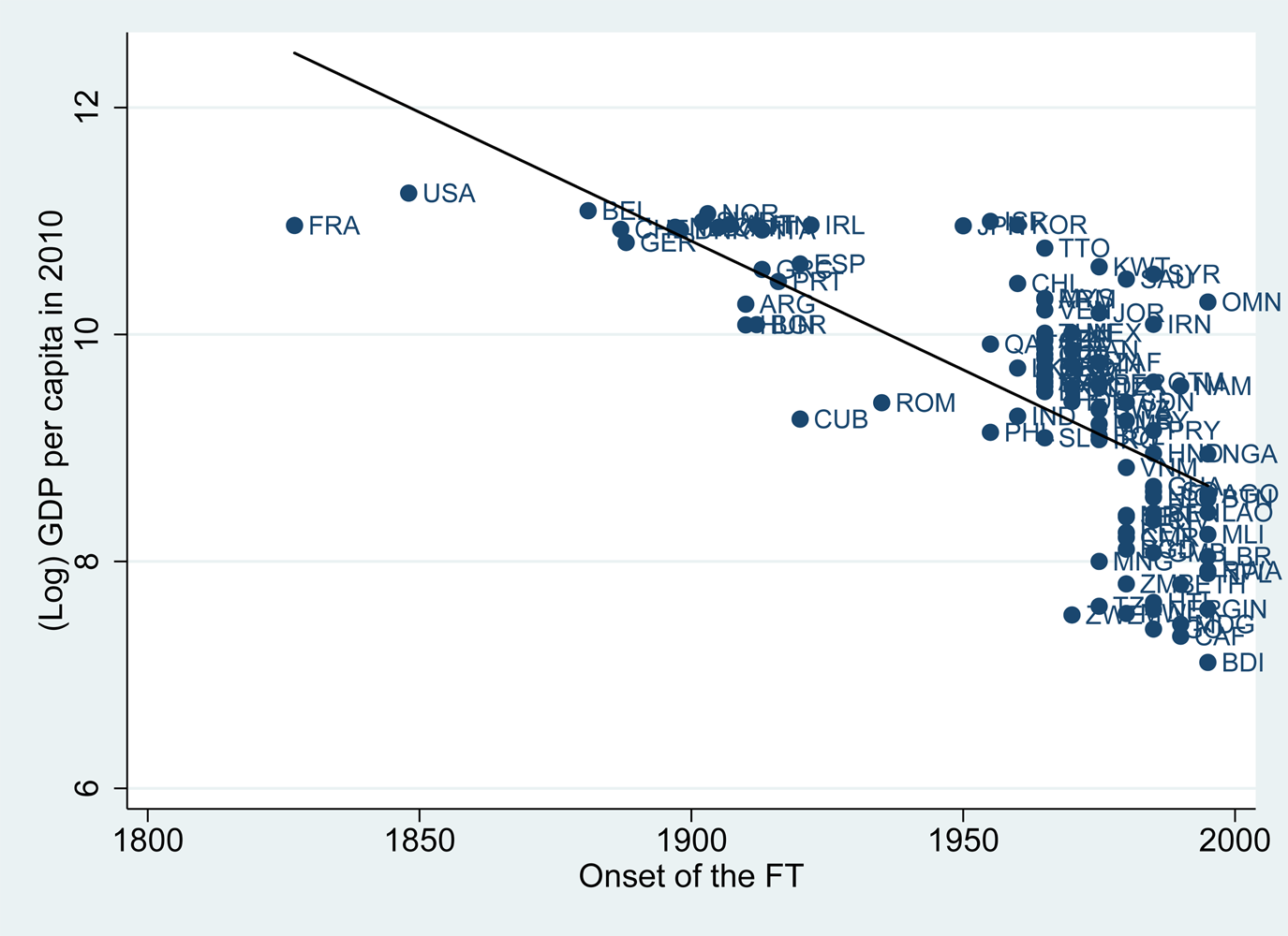
There is now strong consensus among economists that countries that experienced an early demographic transition have better economic outcomes than those that have had a delayed transition, or have not yet completed it, see Galor (Reference Galor2012), Daalgard and Strulik (Reference Daalgard and Strulik2013). The fall in mortality and especially fertility rates during a demographic transition allows parents to invest more heavily in the “quality” of children, and this translates, at the macro level, into a larger stock of human capital and economic growth in the long run. For example, Figure 1, from Basso and Cuberes (Reference Basso and Cuberes2017), illustrates this by showing a negative correlation between per worker output in 2010 and the year at which a country experienced the onset of the fertility transition.
Onset of the fertility transition (FT) and GDP per worker in 2010.

Studying the determinants of the demographic transition seems key to understanding contemporaneous cross-country differences in economic performance. One feature about most accounts of the demographic transition is that they ignore potential externalities. For instance, it is often assumed that mortality rates, if modeled at all, are exogenous. If, instead, they depend negatively on the aggregate stock of human capital in the economy, it is natural to assume that parents do not internalize the effect of their human capital investment decisions on the aggregate mortality rate. Additionally, if there exists some degree of increasing returns to population, it is unlikely that parents take into account the positive effect of increasing their fertility on the economy. As we will show, introducing these externalities has significant effects on the predictions of theories of demographic transitions, and this paper examines the fertility and human capital investment differentials between the equilibrium solution and the ${\rm {\cal A}}$ -efficient solution.Footnote 1 Identifying these gaps would help empirical investigations of institutions and/or cultural traditions that help or hinder a group from coordinating a better outcome. Along these lines, Spolaore and Wacziarg (Reference Spolaore and Wacziarg2014) argue that a country's culture is a key determinant of its fertility rate. Moreover, since institutions and culture are known to be very persistent over time, see Acemoglu et al. (Reference Acemoglu, Johnson and Robinson2001, Reference Acemoglu, Ticchi and Vindigni2011), and Voigtländer and Voth (Reference Voigtländer and Voth2012), studying them and how they affected fertility rates and education choices in pre-industrial time would be a valuable research agenda.
In this paper we consider an overlapping generation framework in which parents care about their own consumption, the expected number of surviving children, as well as a precautionary motive for children and the income of the typical surviving child. We present a theoretical model that characterizes the equilibrium and ${\rm {\cal A}}$ -efficient fertility rate and investment per children. With zero mortality risk, the existence of an agglomeration economy arising from specialization implies that the competitive equilibrium results in too few children and too much human capital investment per child. With higher ${\rm {\cal A}}$
 -efficient fertility, human capital investment will be lower in the ${\rm {\cal A}}$
 -efficient allocation, than the equilibrium allocation. Thus it is possible that future generations of adults will be worse off in the ${\rm {\cal A}}$
 -efficient allocation compared with the population alive in the same generation under the equilibrium allocation. Unlike Golosov et al. (Reference Golosov, Jones and Tertilt2007) and Pérez-Nievas et al. (Reference Pérez-Nievas, Conde-Ruiz and Giménez2019), fertility is not sequential, as all children are born at the same time. Thus comparing welfare of children reduces to comparing the utility of the typical child as an adult in any allocation. Thus whether or not future generations are potentially worse off depends on the income growth rate. If the income growth rate in the ${\rm {\cal A}}$
 -efficient allocation exceeds the income growth rate in the equilibrium allocation, then all future generations are better off under the ${\rm {\cal A}}$
 -efficient allocation. However if the income growth rate in the ${\rm {\cal A}}$
 -efficient allocation is below the income growth rate in the equilibrium allocation, eventually future generations in the equilibrium allocation will be better off than those same generations under the ${\rm {\cal A}}$
 -efficient allocation.Footnote 2
With high-mortality risk the ${\rm {\cal A}}$ -efficient planner, which we define in Section 3, chooses lower fertility and higher human capital investment than the equilibrium solution. This leads to an earlier decline in mortality risk and an earlier fertility decline in the ${\rm {\cal A}}$
 -efficient solution in contrast to the equilibrium solution. The mechanism through which this gap is generated is a strong decrease in the precautionary demand for children as a response to the fall in mortality. These results still hold if one includes coordination costs of specialization. The only difference is that in this case, human capital accumulates faster along the ${\rm {\cal A}}$
 -efficient transition to the balanced growth path.
It is not our view that this paper serves as a substitute for any of the previous demographic transition theories. Instead our point is to illustrate an interesting feature of an ${\rm {\cal A}}$ -efficient solution with multiple externalities. If average human capital lowers mortality, then the ${\rm {\cal A}}$
 -efficient solution will have more rapid human capital accumulation early compared with the equilibrium solution. If in addition there are increasing returns to specialization, and hence increasing returns to population, limited by a human capital coordination technology, then under zero mortality there is a transitional dynamic phase in which ${\rm {\cal A}}$
 -efficient fertility is lower than equilibrium fertility. This phase is characterized by incredibly fast economic growth, and possibly declining population. Our view is that the model presented here is a complement to previous theories.
The paper is organized as follows. The next section presents a summary of the related literature. The theoretical model is developed in Section 3. We analyze both the equilibrium problem and an efficient problem, each with mortality risk. We present comparative statics on the balanced growth path for each equilibrium and efficient problem. Further, we present time series differences between the equilibrium and efficient solutions. Section 4 concludes the paper.
2. Related literature
Our paper relates to three different strands of the literature. The first one is the study of welfare properties associated with fertility and human capital decisions. The concept of an optimal population growth rate and level has long been discussed by Dasgupta (Reference Dasgupta1969), Samuelson (Reference Samuelson1975), Razin and Ben-Zion (Reference Razin and Ben-Zion1975), Nerlove et al. (Reference Nerlove, Razin and Sadka1982, Reference Nerlove, Razin and Sadka1987), Gigliotti (Reference Gigliotti1983), Willis (Reference Willis, Johnson and Lee1987), Zimmermann (Reference Zimmermann1989), and, more recently, Golosov et al. (Reference Golosov, Jones and Tertilt2007). These papers often discuss how to apply the concept of Pareto optimality to questions related to population, acknowledging the possibility that an increase in population by one person may increase the welfare of this individual, even if it decreases the welfare of all the existing population, see Eckstein and Wolpin (Reference Eckstein and Wolpin1985). In our bench mark model with zero mortality, parents maximize a utility function that depends on own consumption, the number of children, and on their children's income. We show that this equilibrium is inefficient because parents do not internalize the positive effect that a larger population and stock of human capital have on next generation's income.
The literature uses different concepts of efficiency, making comparisons difficult. While discussing all these interpretations of efficiency is out of the scope of this paper, we proceed to discuss some prominent definitions of efficiency to illustrate our point. For example, in Dasgupta (Reference Dasgupta1969), efficient fertility means that the sequence of fertility choices solves a Benthamite social welfare maximization problem.Footnote 3 This implies that there exist many efficient allocations, each of them identified by the discount factor appearing in the social welfare function. In Samuelson (Reference Samuelson1975) and Eckstein and Wolpin (Reference Eckstein and Wolpin1985), the efficient fertility corresponds to the allocation that maximizes the utility of a representative agent among all the possible steady states. In contrast, Razin and Ben Zion (Reference Razin and Ben-Zion1975) define optimal fertility as the sequence of fertility choices that maximizes the utility of the dynasty head.
Our concept of efficient fertility follows the recent literature spurred by Golosov et al. (Reference Golosov, Jones and Tertilt2007) who introduce the concept of ${\rm {\cal A}}$ -efficiency. The notion of ${\rm {\cal A}}$
 -efficiency arises from applying the Pareto criterion to those currently alive, i.e., the existing adults. Therefore ${\rm {\cal A}}$
 -dominance only considers the utility of adults in the current period. An allocation ${\rm {\cal Z}}$
 is ${\rm {\cal A}}$
 -efficient if there does not exist an alternative allocation $ {\rm {{\cal Z}}^{\prime}}$
 that makes all current agents alive in both ${\rm {\cal Z}}$
 and ${\rm {{\cal Z}}^{\prime}}$
 better off without making any of these agents worse off. Following this criterion, in our model a symmetric allocation is referred to as ${\rm {\cal A}}$
 -efficient if, at each point in time, it maximizes the utility of those adult agents alive in that period.Footnote 4 As stated above, given the wide range of efficiency definitions used in the literature, it is difficult to compare the pros and cons of using a particular one. However one clear advantage of the ${\rm {\cal A}}$
 -efficiency concept is that, as shown in Schoonbroodt and Tertilt (Reference Schoonbroodt and Tertilt2014) and Conde-Ruiz et al. (Reference Conde-Ruiz, Giménez and Pérez-Nievas2010), the set of symmetric ${\rm {\cal A}}$
 -efficient allocations is much smaller than the class of Benthamite or Millian optima proposed in the literature.Footnote 5
Second, our assumption of increasing returns to population is in line with other research that highlights the role played by high population or population density in the takeoff from a Malthusian economy to sustained growth. For example, Boucekkine et al (Reference Boucekkine, de la Croix and Peeters2007, Reference Boucekkine, de la Croix, Peeters, Prskawetz, Bloom and Lutz2008) argue that the adoption of new technologies in England during the period 1530–1860 was largely facilitated by a high density of educated population. An important difference between these papers and ours is that, in our case, increasing returns to population only matter in the balanced growth path, where we show that a benevolent social planner would choose a higher fertility rate than the competitive equilibrium.
Finally, our paper contributes to the theoretical literature on the demographic transition. Most of the existing papers focus on the triggers of the fertility transition, see Becker (Reference Becker1960); Becker and Lewis (Reference Becker and Lewis1973); Galor and Weil (Reference Galor and Weil1999, Reference Galor and Weil2000); Galor and Moav (Reference Galor and Moav2002), Lagerlöf (Reference Lagerlöf2003).Footnote 6 Our paper explains both the mortality and fertility transitions in a unified framework as in Sah (Reference Sah1991), Fernández-Villaverde (Reference Fernández-Villaverde2001), Kalemli-Ozcan (Reference Kalemli-Ozcan2002), Boldrin and Jones (Reference Boldrin and Jones2002) and Doepke (Reference Doepke2005). In our model the rise in average human capital is what eventually lowers mortality, and the nonlinearity of this relationship produces a rapid mortality decline and subsequently a rapid decline in precautionary fertility by parents.Footnote 7 Our precautionary demand for fertility is similar to Kalemli-Ozcan (Reference Kalemli-Ozcan2002, Reference Kalemli-Ozcan2003), Tamura (Reference Tamura2006), Tamura et al. (Reference Tamura, Simon and Murphy2016) and Tamura and Simon (Reference Tamura and Simon2017).
Another important paper that endogenously links the fall in mortality rates and demographic transitions is Jones (Reference Jones2001). In his model, the occasional generation of new ideas in a Malthusian economy translates into a larger population size. This larger population in turn produces more ideas and this raises consumption per capita, reducing mortality rates and hence triggers a demographic transition. In his model, as in ours, it is the case that, had agents taken into account the positive effects of a larger population, the industrial revolution (and the demographic transition) would have taken place much earlier. However, Jones does not solve for the optimal problem explicitly.
3. Theoretical benchmark
3.1 The baseline model
In this section we construct the micro-foundations for the total factor productivity, TFP, in final goods production. Consider an economy populated by P t workers.Footnote 8 There is a single consumption good which is produced using the human capital of N t workers, where 1 ≤ N t < P t. These N t workers use the following reduced form for the aggregate output:Footnote 9

where Y t is the output at period t and h it is the human capital provided by agent i at period t. The parameter ω >1 represents the degree of increasing returns to population at the aggregate level, arising from specialization returns as in Rosen (Reference Rosen1982) and Tamura (Reference Tamura1992, Reference Tamura2002, Reference Tamura2006). Note that there are diminishing returns to individual human capital since ω is larger than one. However, there is constant returns to the entire distribution of human capital. Within the production coalition, workers are paid the marginal product of their human capital; w jt is the wage per unit of human capital for worker of type j. All workers of type j have the same human capital given by $\bar{h}_{jt}$ . Let y jt be a typical worker j's earnings. Then:

where the last equality arises because in the equilibrium that we assumed $\bar{h}_{jt} = h_{jt}$ , for any j and t. It is evident that earnings of all N t members of the production coalition exactly exhaust output:

This formulation is convenient because it allows us to have increasing returns but also firms that behave competitively, in a similar spirit as in Romer (Reference Romer1986). There are two restrictions on the number of workers in a production coalition. First, it cannot fall below 1, which represents autarky. Second, the number of workers cannot exceed either a size determined by coordination costs, $\lsqb {\sigma {\bar{h}}_t} \rsqb ^\lambda$ where $\bar{h}_t$
 is the average human capital in the production coalition, or a fixed proportion, 0 < ξ ≤ 1, of the total population. Thus we assume:

Thus, while market specialization can increase, that is a rising number of distinct workers cooperating to produce the single consumption good, it can never exceed the population of the world economy. What determines the scope of specialization? Since the number of workers in the production coalition is determined by the average human capital $\bar{h}_t$ , or the population of the world economy, ξP t, there is an external effect of human capital and population. During autarkic production, human capital accumulation does not affect the number of workers within a production coalition. Therefore, absent any other external effects of human capital, there would be no difference in the human capital accumulation of workers in equilibrium versus workers in an efficient allocation. Once production moves out of autarky, N t > 1, there are two long run possibilities. First, the coordination costs may not bind and market coalition is given by N t = ξP t and grows at the rate of population growth. The second possibility is that coordination costs always bind, and $N_t = \lsqb {\sigma {\bar{h}}_t} \rsqb ^\lambda$
 . In this case the market grows at the constant rate equal to the human capital growth rate raised to the λ power, which implies that this is also the rate of growth of the population in the efficient solution. We present more results on the long run balanced growth path in the numerical solutions section.
Returning to production, under symmetry output is given by:

or, in per capita terms

TFP is endogenously determined by the degree of specialization, $Z_t = N_t^{\omega -1}$ . In an equilibrium solution, individuals do not take into account the positive external benefit their human capital accumulation or their fertility provides for future specialization gains. Furthermore, they do not take into account that their human capital is complementary to other workers, nor that their human capital investments for their children have effects on wages of all other workers in that generation. Hence they treat the time path of TFP, Z t, as exogenous technological progress.Footnote 10
3.1.1 Equilibrium model
The economy is populated by individuals who live for two periods, and a family consists of a parent and his children. In the first period individuals receive the education provided by their parent. In the second period they form their own household, work, choose their fertility, and rear and educate their children.
Parents care about their own consumption, c, their expected number of surviving children, x(1 − δ), and the income, y, of their typical child. In addition, with mortality risk, parents are assumed to have a precautionary demand for children.Footnote 11 A parent receives no utility from leisure, so a parent only works or spends time rearing and educating children. Thus the typical generation t parent i maximizes:Footnote 12

The typical t period parent's budget constraint is

where θ > 0 is the unavoidable time cost of child rearing, and τ it is time spent teaching each child. Human capital next period depends on the investment time per child τ it i.e.,

where μ > 0 and A > 1 are efficiency parameters.Footnote 13 We assume that the cumulative mortality of young adults is a declining function of the average human capital of their generation:Footnote 14

where $\bar{h}_{it + 1}$ is the average human capital of adult generation t + 1 and ψ 1 and ψ 2 are positive parameters. Hence whether a child born of a t generation parent, and hence a t + 1 generation adult, survives is an increasing function of the average human capital of their generation.Footnote 15
In the competitive equilibrium we have price taking behavior. Individuals are paid the marginal product of their human capital. The typical parent takes the wage per unit of human capital as given, and does not assume that his/her investment decisions have any effect on this wage, nor on the wage of any other worker. Furthermore the parent does not assume that their education provided to their children affects their child's wage.Footnote 16 Given that the production technology has constant returns to scale in the distribution of human capital in the economy, paying each worker their marginal product exactly exhausts output, which is evident from summing over all worker types in (2). Focusing only on the choice variables of a parent, the equilibrium problem for parent i in generation t can be written as:Footnote 17

The first order conditions with respect to fertility and human capital investment produce the following expressions.


Observe that the first order condition for human capital investment in the equilibrium model is independent of mortality; the only way in which mortality risk affects human capital investment is indirectly through the fertility choice. Because of the non-convexity in the budget constraint induced by the quality–quantity interaction of (x it, τ it), we solve this problem using a grid on human capital investment rates given by:Footnote 18

Then for each value of τ s and imposing the homogeneity of the parents, we compute the mortality rate for these young adults using (8). We use (10) to solve for the fertility choice for each τ s on the grid.Footnote 19 If we define m = δ/(2(1 − δ)), then it is easy to show that (∂x/∂m) > 0. So in a world with mortality risk, for any choice of human capital investment, fertility is higher than in a world with no mortality risk. After solving for the fertility choice as a function of the investment rate, we verify that (11) holds. We discard those solutions that do not satisfy this equilibrium first order condition.Footnote 20 From this reduced set of investment and fertility candidate pairs, the utility maximizing choice is selected.
3.1.2 Equilibrium solution: zero mortality
Here we solve for the stationary zero mortality equilibrium solution. Using (10) it is easy to show that the fraction of resources spent on the next generation is constant and equal to 1 − α. Combining the results in (10) and (11), we find the equilibrium stationary fertility and investment time:


In order to have a meaningful equilibrium we impose:

Intuitively, an increase in β—i.e., if parents care more about their children's income—reduces fertility and increases the investment in children's human capital. Similarly, a higher θ reduces fertility and increases investment per child since the fixed cost of rearing a child is now higher. Finally, an increase in μ also increases investment in children's human capital, since the return to this investment is now higher.Footnote 21
3.1.3 ${\rm {\cal A}}$ -Efficient model

In the ${\rm {\cal A}}$ -efficient model, we consider the case in which a social planner internalizes the positive externality of population growth on TFP growth, as well as the positive externality of human capital investment on the next generation wages and next generation mortality risk. It is better to think of the planner's problem as actually an infinite sequence of separate planners.Footnote 22 In a given period, the planning problem maximizes the summation of the welfare of adults. The planner chooses the consumption for all adults in the coalition, their fertility, and their human capital investment in each child, but does not choose the number of grandchildren, nor the investment of human capital in the grandchildren. However, the planner does internalize the external effects of current fertility on the population next period and production, and also the effects of human capital of the next generation on the production coalition size and hence wages of that generation. The planner also considers the effect of human capital investment on the mortality risk facing the children, although the planner does not internalize the effect of the investment on the cost of human capital accumulation for the current parent's grandchildren.Footnote 23 For convenience, and without loss of generality, we focus on the efficient solution in which all parents are treated equally. Thus in our analysis of the efficient solution, we are using the notion of ${\rm {\cal A}}$
 -efficiency of Golosov et al. (Reference Golosov, Jones and Tertilt2007): an allocation of (c t, x t, h t+1) is ${\rm {\cal A}}$
 -efficient if there does not exist another allocation $\lpar {c_t^{\prime}, x_t^{\prime}, h_{t + 1}^{\prime}} \rpar$
 that makes any subset of the adult population better off without making any adult worse off.Footnote 24
Here we solve the planner's problem, and we only examine the case with identical individuals. We focus on the equal weight solution, and hence the representative parent. There are several regions that must be solved in order to characterize the efficient path. In the earliest days, human capital will be sufficiently low that no specialization occurs, and hence autarky is the method of production. Human capital accumulation may affect the mortality of the young adult, but not determine the scale of the production coalition. In the final stage, either the coordination technology will determine the size of the production coalition, or it will be determined by the fixed proportion of the total population, determined in (4). Since all individuals are identical, the earnings of a typical worker are given by:


The planner's problem can be written as:Footnote 25

The first order conditions for fertility and human capital investment are:


If human capital of the child does not affect his or her mortality rate, that is h t+1 is below the critical threshold, and if ∂N t+1/∂x t = 0 and ∂N t+1/∂h t+1 = 0, then the two first order conditions of the social planner are identical to the first order conditions in the equilibrium solution. Thus for the earliest part of history, there is no difference in the path of human capital taken in the equilibrium solution and the efficient solution.
Now consider the range where children's human capital reduces their mortality, ∂δ/∂τ t < 0. We further assume that the market size could be larger than autarky in the children's adulthood, i.e., N t+1 >1. We use the same solution algorithm to solve for the ${\rm {\cal A}}$ -efficient choice of fertility and human capital investment as we used in solving for the equilibrium choices. We use the same grid on possible investment rates, τ t and the implied young adult mortality rate as in our equilibrium solution, see (12) and (8). For each value of τ s, the first order condition for ${\rm {\cal A}}$
 -efficient fertility is given by (15). If the production coalition is determined by the evolution of population, then the first order condition for fertility can be written as:

For any given investment rate τ s, this is a quadratic function in x s. Appendix B contains the exact form and the solution under this regime.
For each (τ s, x s) pair, we compute the utility of the representative parent, and the potential ${\rm {\cal A}}$ -efficient solution is the maximizing pair. Unlike in the equilibrium solution, we do not constrain the choice of investment other than its feasibility. Implicitly the investment rate either satisfies (16) if interior, or is a corner solution. In either case, it is generally not equal to the equilibrium choice as (11) and (16) are not identical.
If the production coalition is determined by the coordination technology, i.e., 1 < N t+1 = [σh t+1]λ < ξP t+1, then the first order condition for fertility can be written as:

For this case, Appendix C presents the quadratic form that fertility solves for any choice of τ s. The solution, under the assumption that the production coalition is determined by the coordination technology, is the (x s,τ s) that maximizes the utility of the representative parent.
We take the two candidate solutions from above, population is the determining coalition size, or if the coordination technology is the coalition size, and whichever regime maximizes the utility of the typical parent is the ${\rm {\cal A}}$ -efficient solution.
For both the equilibrium solution and the ${\rm {\cal A}}$ -efficient solution, we produce the time series on population, fertility, mortality, human capital, coalition size, and real per capita output. The evolution is given by:


where r refers to either equilibrium or ${\rm {\cal A}}$-efficient solutions.
3.1.4 ${\rm {\cal A}}$-Efficient model: zero mortality

In this section we characterize the zero mortality ${\rm {\cal A}}$ -efficient solution. There are three possibilities, one of which we ignore for simple reasons. These solutions depend on the long run growth rate of the production coalition. One possibility is that the coalition grows at the stationary rate of fertility, x, and that the coordination costs are never binding: ξP t+1 = ξP tx = N tx = N t+1 <[σAh tτ μ]λ = [σh t+1]λ. A second possibility is that the coordination costs are always binding, and fertility is equal to the growth rate of the coalition arising from declining coordination costs: x = [Aτ μ]λ, N t+1 < ξP tx. Finally, the third case is that the coordination costs determine the coalition size, and fertility exceeds the growth rate of the coalition: x > [Aτ μ]λ, N t+1 < ξP tx. We disregard this third possibility as the fertility rate is below the rate of the equilibrium fertility in the scenario with zero mortality.Footnote 26
In the first case, the ${\rm {\cal A}}$ -efficient solution is characterized by the following first order conditions:


Solving these equations for the ${\rm {\cal A}}$ -efficient solutions for fertility and investment produces:


It is clear that an increase in ω − 1 induces a higher fertility rate since the positive external effect of population on output per capita and wages is now higher. The corresponding level of investment per child decreases as ω − 1 increases. Utilizing (13) and (14), it is also easy to show that x eff > x eq and τ eff < τ eq.
In the second case, the solution requires that fertility be equal to the growth rate of the production coalition arising from the coordination costs. Thus we have:

The ${\rm {\cal A}}$ -efficient problem facing the planner becomes:

The first order condition for the optimal human capital investment rate is:

We solve for both possible solutions (production coalition grows at the rate of fertility, and the production coalition is given by the coordination technology), and compare the utility attained by the representative household under each solution. The ${\rm {\cal A}}$ -efficient solution arises from the maximum of these two possibilities. In our solutions, with small agglomeration returns to specialization, ω between 1.01 and 1.20, the first solution is optimal. In all other numerical solutions, the ${\rm {\cal A}}$
 -efficient solution corresponds to the second case, with human capital investment, τ, given by (21).
Table 1 contains the values of the parameters used for the numerical solutions. We used (13) and (14), and assumed stationary equilibrium fertility of x eq = 1.000000001 and τ eq = 0.375. The stationary equilibrium fertility is one of near stationary population. We chose this as the current rich countries are all below replacement fertility today, but we forecast that stationary population is more likely. Second, assuming that a period is 40 years, the equilibrium schooling is given by 40τ eq = 15, i.e., we assume that stationary equilibrium fertility is slightly less than college graduation. This is consistent with the 15 years of schooling of the 2010 generation in Denmark, Finland, Iceland, New Zealand, and the United States using the data from Tamura et al. (Reference Tamura, Dwyer, Devereux and Baier2019). In addition our choices of α, β, θ, and μ are designed to produce the following equilibrium balanced growth path outcomes: annual discount rate of β .025 = 0.9767, biological maximum fertility of (1/θ) = 11.4, and long run annualized per capita income growth of 1.7%, or a doubling of living standards every generation.
Parameter values

3.1.5 Comparing both setups under zero mortality
Here we present the stationary solutions for both the equilibrium solution and the ${\rm {\cal A}}$ -efficient solution. While analytical solutions are available for the equilibrium solution and the first case in the ${\rm {\cal A}}$
 -efficient solution, the typical ${\rm {\cal A}}$
 -efficient solution is not analytical. Thus to facilitate the comparison between the equilibrium model and ${\rm {\cal A}}$
 -efficient model solutions, we present the stationary outcomes graphically. In the following figures, we present the stationary annualized income growth rates, fertility, and schooling as functions of the coordination cost parameter, λ, and the agglomeration returns to specialization, ω.
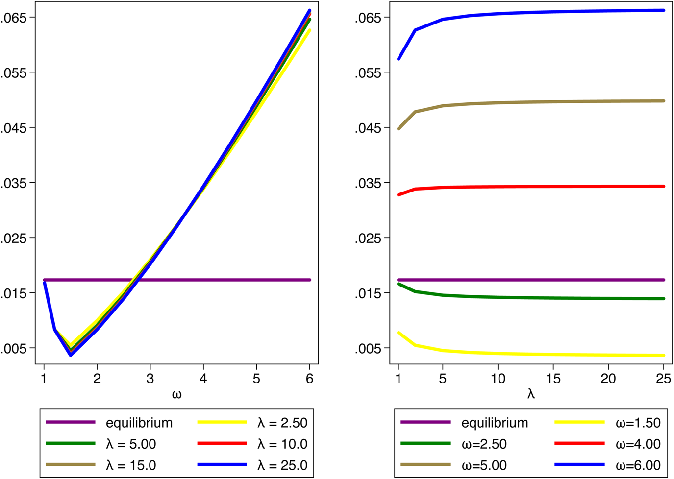
In Figure 2 we present two panels; the left side shows the stationary annualized income growth rate as a function of ω, and the right side shows the stationary annualized income growth rate as a function of λ. Observe that for fixed λ, the ${\rm {\cal A}}$ -efficient income growth rate is non-monotonic in ω; it first falls until ω = 1.5, and then increases for higher values. Similarly, for fixed ω, the A-efficient income growth rate is monotonic in λ, but the relationship changes sign. For our ${\rm {\cal A}}$
 -efficient model solutions and ω < 3.5, ${\rm {\cal A}}$
 -efficient income growth is a decreasing function of λ. However, for higher values of ω, ${\rm {\cal A}}$
 -efficient income growth is monotonically increasing in λ. Notice that the equilibrium income growth rate exceeds the ${\rm {\cal A}}$
 -efficient income growth rate for all values of λ and ω < 2.75. For higher agglomeration returns to specialization, the ${\rm {\cal A}}$
 -efficient income growth rate exceeds the equilibrium income growth rate. As mentioned above, when the per capita income growth rate in the ${\rm {\cal A}}$
 -efficient allocation exceeds the per capita income growth rate in the equilibrium allocation, and all future generations have higher utility than their equilibrium counterparts.
Stationary equilibrium and ${\rm {\cal A}}$ -efficient annualized per capita income growth rates.

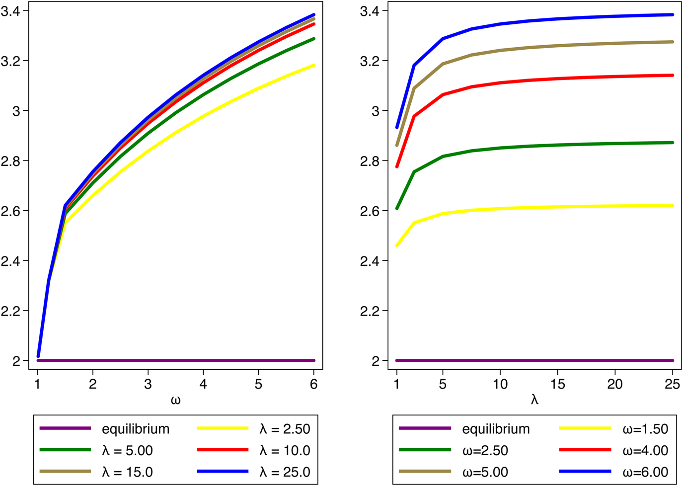
Figure 3 presents the stationary equilibrium fertility, and stationary ${\rm {\cal A}}$ -efficient fertility for varying values for λ and ω. Stationary equilibrium fertility is independent of both ω and λ, because parents only get utility from children, and do not internalize the external benefit of population on earnings. For all values of these two parameters, stationary ${\rm {\cal A}}$
 -efficient fertility is higher than stationary equilibrium fertility. This is not a surprise, since at zero mortality, the equilibrium return to children comes only from the direct utility of having children, whereas for the ${\rm {\cal A}}$
 -efficient solution, it internalizes the externality on the next generation's earnings. Unlike the growth rate results, stationary ${\rm {\cal A}}$
 -efficient fertility is increasing in both λ and ω. In both cases, higher values of λ and ω increase the positive external benefit of population on earnings, and hence leads the ${\rm {\cal A}}$
 -efficient planner to increase stationary fertility.
Stationary equilibrium and ${\rm {\cal A}}$ -efficient fertility.

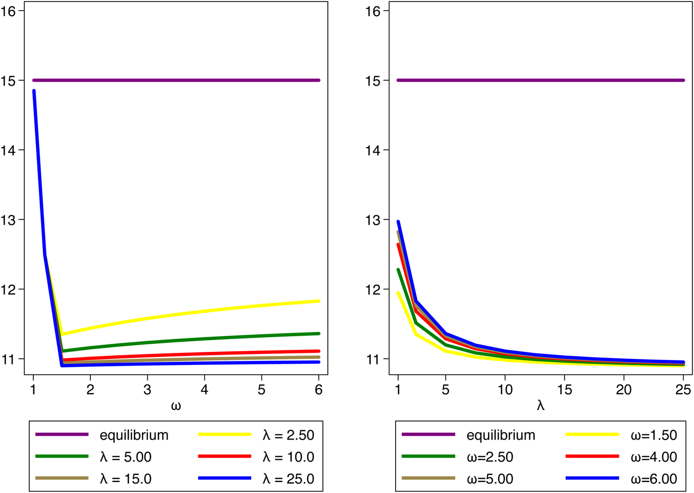
Figure 4 presents the stationary equilibrium schooling and stationary ${\rm {\cal A}}$ -efficient schooling for varying values for λ and ω. As with fertility, the stationary equilibrium schooling is independent of both ω and λ. Unlike its fertility counterpart, stationary ${\rm {\cal A}}$
 -efficient schooling is not monotonically related to ω. For all values of λ, as the agglomeration return to specialization increases from slightly bigger than 1, to around 1.5, stationary ${\rm {\cal A}}$
 -efficient schooling declines. Nevertheless, once it reaches its minimum value, stationary ${\rm {\cal A}}$
 -efficient schooling is increasing in ω. For all values of λ between 1 and 25, stationary ${\rm {\cal A}}$
 -efficient schooling is increasing in ω for ω > 1.5. On the other hand, for all values of ω, stationary ${\rm {\cal A}}$
 -efficient schooling is monotonically decreasing in λ. The stationary ${\rm {\cal A}}$
 -efficient schooling comparative statics mirror the stationary ${\rm {\cal A}}$
 -efficient income growth comparative statics.
Stationary equilibrium and ${\rm {\cal A}}$ -efficient schooling.

3.1.6 Numerical solutions including non-zero mortality
In this section we present numerical solutions to compare and contrast the equilibrium time series with the ${\rm {\cal A}}$ -efficient time series. One interesting feature displayed is the interplay between human capital growth and growth of the production coalition. If the long run coalition is bounded by the coordination cost, that is 1 < N t = [σh t]λ < ξP t, then even with high gains from specialization, a large ω, fertility in the ${\rm {\cal A}}$
 -efficient solution will not be given by (21), but rather x eff = [Aτ μ]λ. If the long run coalition is bounded by the maximum fraction of the population, 1 < N t = ξP t < [σh t]λ, then fertility in the efficient solution will be given by (21).
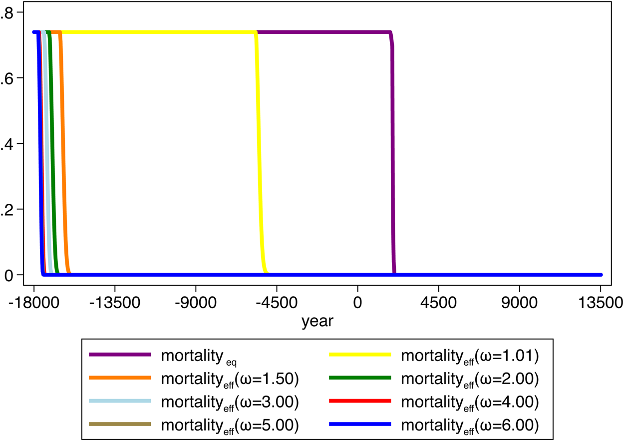
We calibrate the equilibrium model to produce a demographic transition starting in 1800 and terminating in 2080.Footnote 27 For all values of λ and ω, the equilibrium time series on human capital is identical, which implies that the mortality time series is also identical to all λ and ω. Thus the time series on mortality and fertility are independent of λ and ω.Footnote 28 In all figures the equilibrium case assumes ω = 1.01 and λ = 2.5. By contrast, for all values of ω, the ${\rm {\cal A}}$ -efficient solution has an earlier acceleration in growth, and a much earlier decline in mortality. The time series of mortality is presented in Figure 5. In the slowest case, ω = 1.01, the mortality decline begins in 5,680 BC, and is completed in 3,800 BC. However, for the next slowest case, both ω = 1.20 and ω = 1.50, the mortality decline begins in 16,560 BC and is completed in 15,360 BC. For ω = 2.00, the mortality decline begins in 17,160 BC and is completed in 16,160 BC. For ω = 6.00, the mortality decline begins in 17,760 BC and is complete in 17,360 BC. So as the returns to agglomeration from specialization increase from 1.01 to 6.00, the mortality decline begins 12,000 years earlier. It also becomes more rapid, dropping from 1880 years in length to 400 years in length. Higher ω increases the return to specialization and population. The ${\rm {\cal A}}$
 -efficient planner internalizes this by accelerating human capital accumulation to lower the coordinating costs of specialization. By accelerating human capital accumulation, the production coalition grows and additionally mortality can decline more rapidly. In all cases the ${\rm {\cal A}}$
 -efficient mortality declines occur and end before the equilibrium mortality decline. The onset is at worst only 7500 years earlier, and in the extreme case almost 20,000 years earlier.
Equilibrium and ${\rm {\cal A}}$ -efficient mortality.

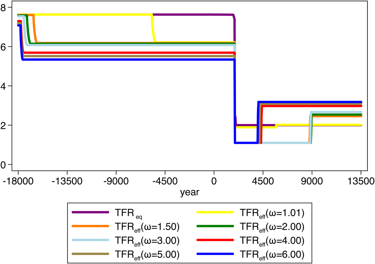
Figure 6 shows the time series of total fertility rates. We produced total fertility rates by multiplying fertility in the model solutions by 2. The equilibrium time series path of total fertility reproduces the long classical-Malthusian world, interrupted by a brief and rapid fertility transition, and followed by a stationary total fertility rate of near zero population growth. This equilibrium fertility time series is identical across all values of ω. In all cases presented of ${\rm {\cal A}}$ -efficient fertility, fertility actually is below the equilibrium fertility during the high-mortality regime, and even through the fertility transition in the equilibrium time series. With lower fertility comes the more rapid human capital accumulation as the planner internalizes the benefit of human capital accumulation in reducing young adult mortality. With the earlier onset of the ${\rm {\cal A}}$
 -efficient mortality decline, the ${\rm {\cal A}}$
 -efficient fertility declines to a new stationary value that also looks classical. About the time of the equilibrium fertility transition there is another large decline in the ${\rm {\cal A}}$
 -efficient fertility. This period corresponds to an ${\rm {\cal A}}$
 -efficient transition dynamic phase. Because world population is so much larger than the ${\rm {\cal A}}$
 -efficient production coalition, this period is marked by an extremely high rate of human capital investment and actual population decline. This period is also characterized by rapid growth in the size of the production coalition (much more rapid than stationary ${\rm {\cal A}}$
 -efficient fertility) and extremely high-transitional dynamic income growth rates. Finally, once human capital is sufficiently large that the production coalition is determined by ζP t, then the stationary ${\rm {\cal A}}$
 -efficient fertility and human capital investment period are observed. In this phase, the ${\rm {\cal A}}$
 -efficient fertility exceeds the equilibrium fertility for all values of ω.
Equilibrium and ${\rm {\cal A}}$ -efficient total fertility rates.

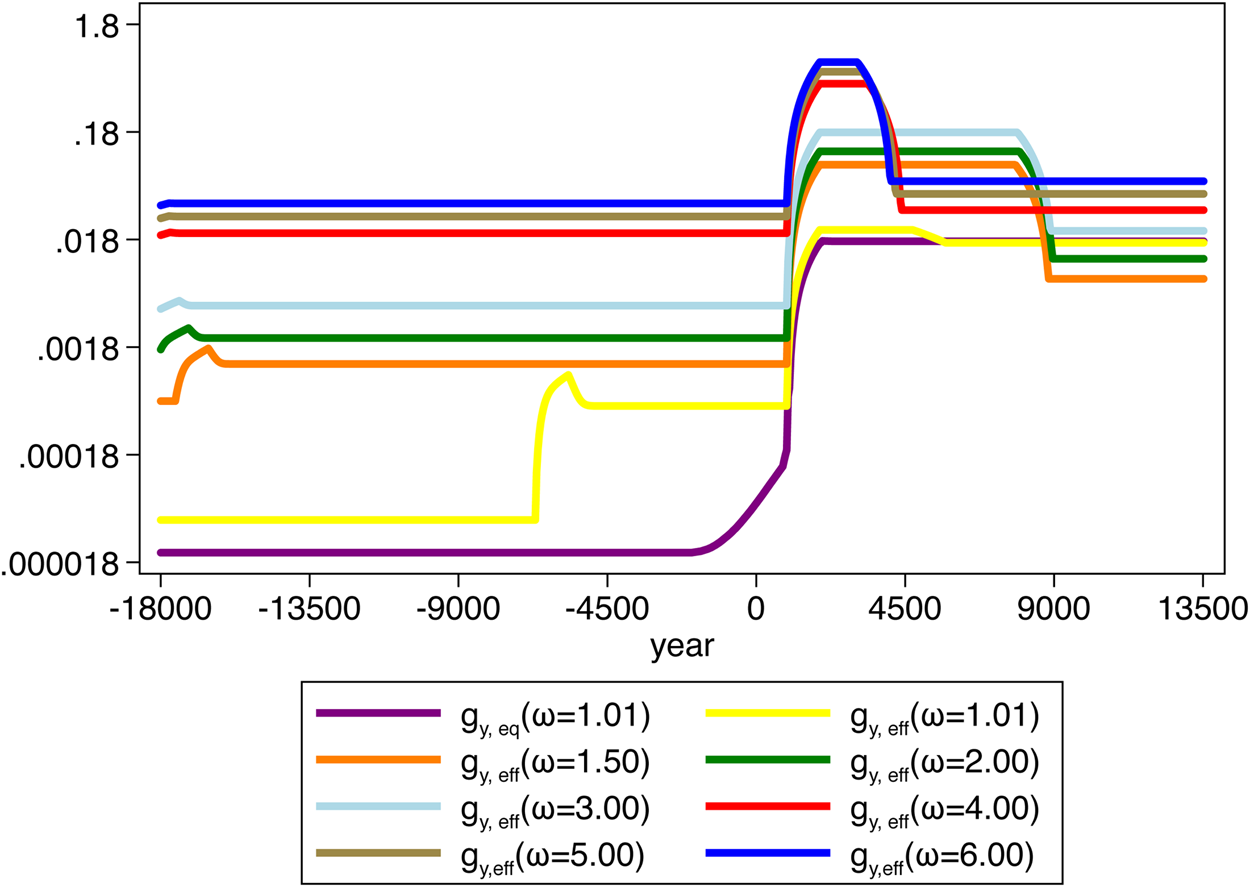
Transition dynamics produce extremely high ${\rm {\cal A}}$ -efficient per capita income growth rates. In order to keep things in scale, we constructed annualized growth rates over 1000 years.Footnote 29 Thus each observation is given by:

where t represents adults in generation t, and each period is 40 years. Figure 7 shows the time series of the per capita income growth rates for the equilibrium solution and the ${\rm {\cal A}}$ -efficient solutions. As mentioned above, during the transition dynamic phase of the ${\rm {\cal A}}$
 -efficient solution, human capital growth is above the stationary value and the growth rate of the production coalition is much greater than fertility. We plotted the growth rates on the log scale in order to show the differences in growth rates for the different values of ω more clearly.Footnote 30
Equilibrium and ${\rm {\cal A}}$ -efficient growth rates of per capita income.

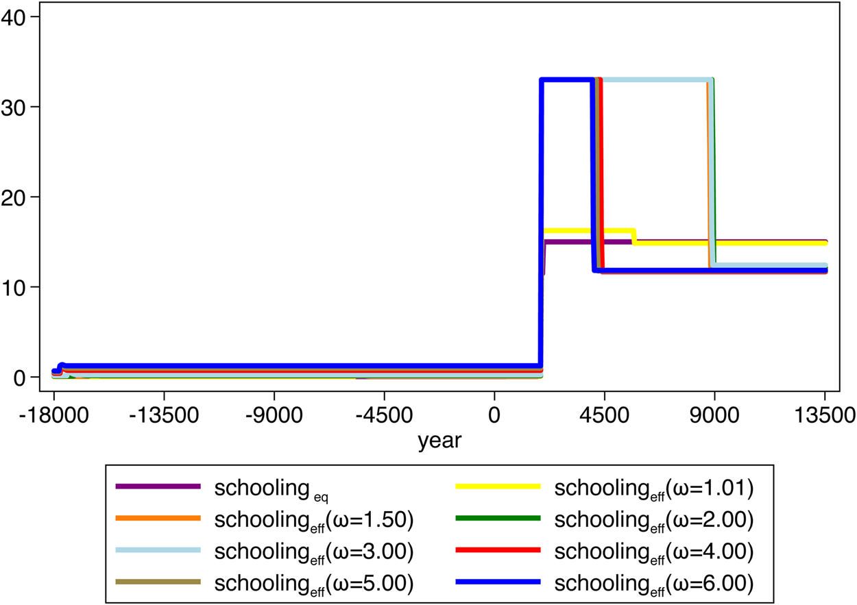
During the demographic transition, the ${\rm {\cal A}}$ -efficient investment in human capital is much larger than the stationary value. Schooling is given by 40τ, and during the transition dynamic phase, the ${\rm {\cal A}}$
 -efficient schooling is at a boundary, that is to say, the planner chooses schooling just slightly below 40(1 − θ). In our solution this is roughly 33 years. This is presented in Figure 8.
Equilibrium and efficient schooling.

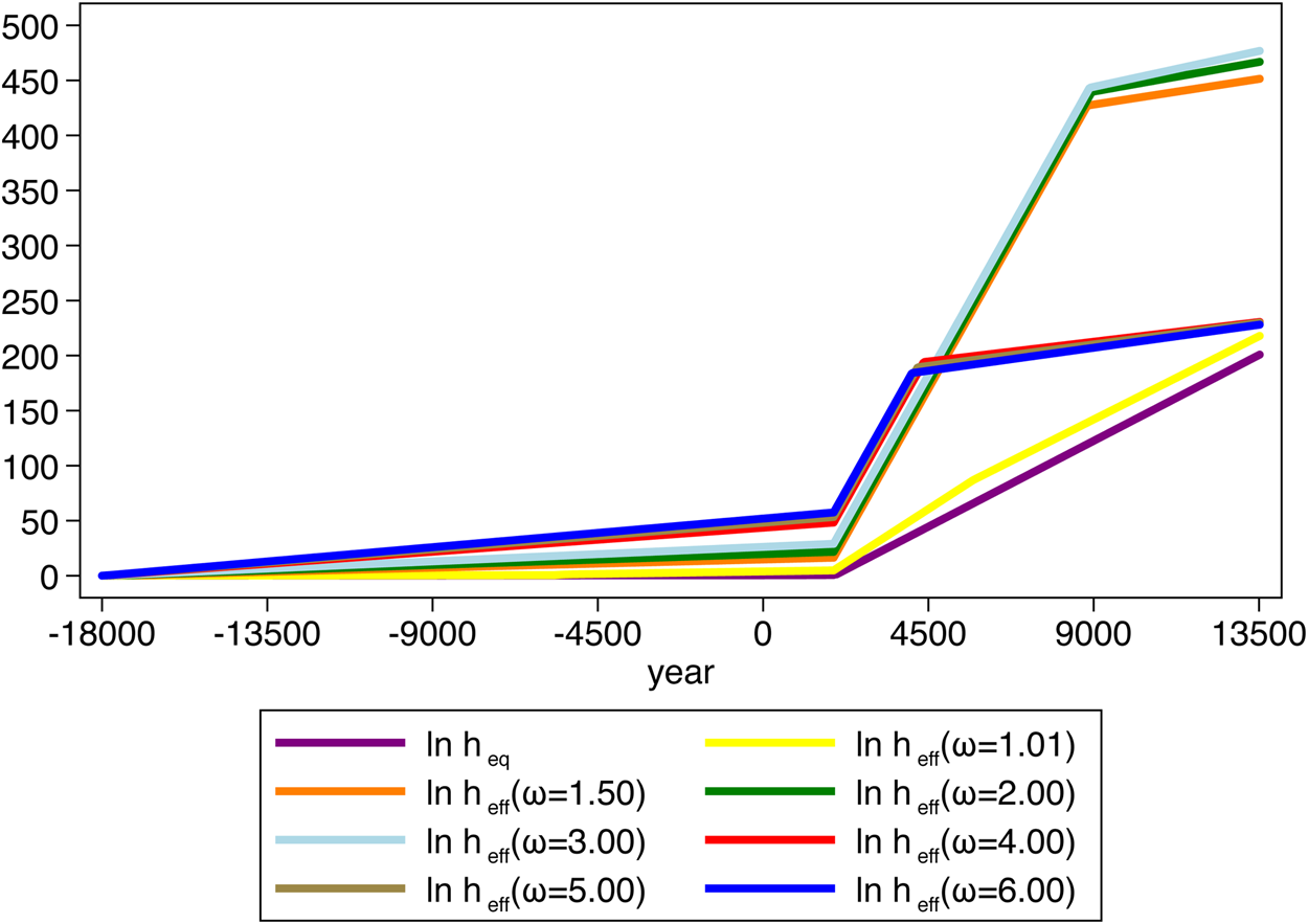
Figure 9 shows the time series for log human capital. It is apparent that the demographic transition has accelerated human capital investment in the ${\rm {\cal A}}$ -efficient solution before falling to a lower balanced growth path value.
Equilibrium and ${\rm {\cal A}}$ -efficient log human capital.

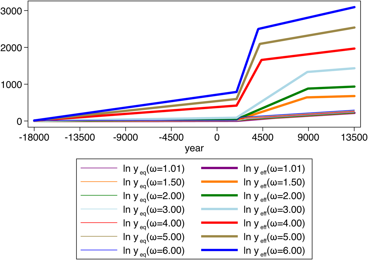
Figure 10 presents the time series of the log per capita output for the equilibrium solution and the ${\rm {\cal A}}$ -efficient solutions. Reflecting the previous results on the growth rate of per capita output, the graph shows the acceleration in per capita income growth during the transition dynamics.
Equilibrium and ${\rm {\cal A}}$ -efficient log per capita output.

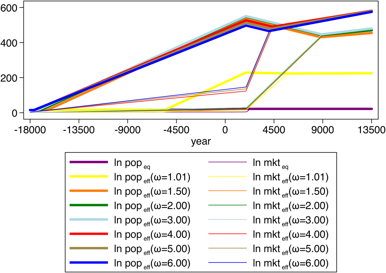
Finally, Figure 11 presents the time series of log population for the equilibrium solution and the equilibrium log production coalition, as well as the log ${\rm {\cal A}}$ -efficient populations and log ${\rm {\cal A}}$
 -efficient production coalitions. The thick lines are the log population curves; one for the equilibrium case, and the others for different ω ${\rm {\cal A}}$
 -efficient time series. In all cases the thinner lines of the same color as the thick lines represent the corresponding log production coalition sizes. We observe that in the transition dynamic phase of the ${\rm {\cal A}}$
 -efficient solutions, log populations are declining, while the log production coalition sizes are growing more rapidly than stationary fertility.
Equilibrium and ${\rm {\cal A}}$ -efficient log population and log production coalition.

4. Conclusion
We develop a model in which the aggregate production function exhibits increasing returns to population. Moreover, individuals have a precautionary demand for children when young adult mortality risk is non-zero. These two assumptions result in an equilibrium fertility rate that is sub-optimal and too much investment in human capital per child in equilibrium in the long run. We characterize the gap between equilibrium and ${\rm {\cal A}}$ -efficient fertility and investment in human capital, with and without mortality of young adults. When we add young adult mortality to the model we find that the ${\rm {\cal A}}$
 -efficient solution of the model involves accumulating human capital rapidly to eliminate mortality quickly. Our numerical solutions indicate that the ${\rm {\cal A}}$
 -efficient solution produces zero mortality as much as 20,000 years before it occurs in the equilibrium solution. This leads to an early intermediate fertility transition, although ${\rm {\cal A}}$
 -efficient fertility in the long run increases again above the equilibrium level to take advantage of the increasing returns in population. The model presented here provides a unified framework to understand fertility and mortality in a dynamic context, and allows us to establish a clear comparison between the equilibrium and ${\rm {\cal A}}$
 -efficient paths of the two variables. The comparison can guide future empirical investigations of the causes and effects of demographic transitions experienced by different countries in the world.
Acknowledgements
We thank the editor and two anonymous referees, Michal Jerzmanowski, Kevin Tsui, and seminar participants at University of Barcelona, University of Vigo, GREQAM (Marseille), and the 2013 Warwick Summer School for useful comments. All remaining errors are ours.
Appendix A
In this appendix we present the quadratic equation that determines equilibrium fertility for each potential choice of equilibrium human capital investment choice, τ st. The fertility choice, x st, for a given investment rate, τ s, solves the following quadratic equation:

Thus for each potential equilibrium human capital investment choice, τ st, there is a unique equilibrium fertility choice. To choose among all possible pairs, (x st, τ st), we require that they also solve (12). That is a parent chooses fertility and investment without taking into account the external effect of either on production specialization and mortality. Comparing the candidate (x st, τ st) pairs, the equilibrium choice is one that maximizes the parent's utility, imposing the equilibrium conditions on mortality δ st and technology.
Appendix B

If the production coalition is a constant fraction of the population, and hence the growth of the production coalition is given by the growth rate of population, the solution is given by:

For the candidate pairs(x st, τ st), the optimal choice in this regime maximizes the utility of the typical parent.
Appendix C

In the case where the production coalition growth is determined by the coordination technology, for each investment rate τ it, the first order condition of fertility is a quadratic form given by:

The solution is the (τ s, x s) pair that maximizes utility.