1. Introduction
The literature makes clear that income takes a permanent drop after an involuntary job displacement, but it has not been clear what happens to long run wealth in the USA.Footnote 1 The level of wealth is an important backdrop for nearly every choice made by a household. Therefore, understanding this topic is at the heart of several issues in economics and beyond. Households may respond to a drop in income by decreasing consumption and/or decreasing their wealth. For example, a permanent drop in income by the highest earner for a household may be met with a change in consumption behavior which would result in small impacts for wealth. The opposite could occur where a drop in income may lead to a depletion of wealth if the household is unable to change its consumption patterns. This article helps provide clarity on this by documenting the effect that displacement has on long run wealth and consumption.
Involuntary job displacement leads to decreases in relative wealth with no signs of recovery. Upon first displacement, wealth including home equity is 14% lower than workers with similar characteristics from the Panel Study of Income Dynamics (PSID).Footnote 2 This wealth is still 18% lower when it has been at least 12 years since the event. The fall in wealth excluding home equity is similar with the initial fall being 16% and the lasting effect at 23%. These results are robust to different specifications and transformations. This article also examines the various components of wealth and finds that no one component is driving the wealth results.
Consumption has a much smaller relative fall after involuntary job displacement. Specifically, households consume 2% less upon displacement and 4% less 12 years later. However, these differences are not statistically significant at the 5% level. The lack of a significant fall in consumption also holds for food consumption which is different than previous research on the topic and is explored in this article.
A general life cycle model does not match this behavior. The model from Carroll (Reference Carroll2012) calibrated to US data suggests that workers should have a large initial drop in wealth but that there should also be recovery. The recovery exists in the model even though the parameters are estimated to successfully reproduce a lasting income drop like that found in the PSID. The model has a drop in consumption and while this occurs in the data, the difference is in the magnitudes. An extension of the life cycle model to include habit formation with last period’s consumption in the utility function improves the fit with the data. While the differences in magnitudes for consumption remain, this extension has nearly the same long run implications on wealth. This allows for the examination of wealth at the time of death providing insight on what to expect from bequests.
These results are an important contribution to the literature since it documents the long run impact that involuntary job displacement has on wealth, consumption, and income for a representative sample in the USA. The empirical results are also put in direct context of theoretical expectations. These are contributions because the research done in this area examines short-term impacts due to data limitations in the early data. Additionally, the literature on these topics either involves data from different countries or is based on data that is not representative of the USA.
The results of this article fill a gap in the literature and indicate that the typical experience for average-aged workers in the USA is worse than previous studies that used different data. For example, Basten et al. (Reference Basten, Fagereng and Telle2016) show that workers who experienced mass layoffs in Norway deplete 11–12% of their wealth in the 2–4 years after the event. Earlier work for the USA involves the Health and Retirement Study (HRS) of workers aged 50–61 and their spouses. Stevens and Moulton (Reference Stevens and Moulton2013) use the HRS to show that these workers who experience job displacement experience wealth losses of 8–13% seven or more years after the event. Ozturk and Gallo (Reference Ozturk and Gallo2013) is a working paper that also uses the HRS to show that displaced workers that are at least 51 years old experience an 8% reduction in wealth compared to similar workers without this type of job loss.Footnote 3 This work also complements Gruber (Reference Gruber2001) and Dickens et al. (Reference Dickens, Triest and Sederberg2017) who use the Survey of Income and Program Participation (SIPP) to examine wealth that is available to unemployed workers and how this has changed over the decades.
The consumption findings in this article build off Stephens Jr (Reference Stephens2001) by going beyond food consumption which was that paper’s focus. In 1999, the PSID made a major change to its data collection on consumption. The data now goes beyond food to include 70% of all consumption items from the Consumer Expenditure Survey as noted in Blundell et al. (Reference Blundell, Pistaferri and Saporta-Eksten2016). Whereas Stephens Jr (Reference Stephens2001) finds that displacement leads to a 9.75% decrease in food consumption, the findings in this article using the new data suggest smaller decreases in the range of 3–4%.
The next section describes the PSID data that is used for this project before examining the estimation strategy and those results. The following section is the theoretical model with details on the simulation, the model’s results, alternative calibration strategies, and followed with a conclusion.
2. PSID data
This study involves 5169 heads of households from the nationally representative sample designed by the Survey Research Center for the PSID (2020). Each head in this study has reported information on wealth to the PSID at least twice.
The numbers of heads are somewhat smaller than typical PSID studies because the PSID only collected wealth information in 1984, 1989, 1994, and every 2 years starting in 1999 through 2017. Additionally, this article follows Stephens Jr (Reference Stephens2001) and Cagetti (Reference Cagetti2003) in limiting the sample to heads with a partner that is typically present. If a divorce takes place, the rest of the observations for that head are removed from this study.Footnote 4 To understand the effect of displacement for workers in their prime working years, this article also limits the data to heads of the households aged 25– 60 years old for the majority of the article.Footnote 5
The wealth variables are key dependent variables in this study. They vary between wealth with home equity, wealth without the equity, home equity alone, and the other components of wealth. Debt is the total debt calculated by the PSID and this is available in every year noted above. In later waves, the PSID details that this debt is made up of credit card debt, student loan debt, medical debt, legal bills, debt related to business or farming, debt from real estate other than the main home, family loans along with any other type of debt that the family may have. The wealth variables account for the debt just mentioned along with the net value of a business or farm, the sum of checking and savings accounts, the net value of real estate, the value of stocks, the net value of vehicles, and the value of a host of assets such as bonds, life insurance, trusts, estates, collections, private annuities, and individual retirement accounts (IRAs). Additionally, wealth for the household includes the money in all pensions and/or employer-based retirement plans. The individual components of wealth are available in every year noted above except for IRAs being individually unavailable in 1984, 1989, and 1994. However, the PSID collects the value of “other assets” in every year that wealth is collected.
The last dependent variable is total consumption which is also made up of several components. For this article, consumption is based on household expenditures on child care, education, food, health care, housing, and transportation. Following Blundell et al. (Reference Blundell, Pistaferri and Saporta-Eksten2016), missing components are counted as zeros before aggregation. All six consumption components are available in each wave of the PSID starting in 1999–2017.Footnote 6
Income is an important independent variable and like the previous variables, it is made up of several components. These components include the labor part of farm income, the labor part of business income, wages from main jobs, the labor part of market gardening income, the labor part of roomers and boarders income, income from professional practices or trade, bonuses, overtime, commissions, tips, wages from extra jobs along with other job-related income. This variable is available for the head of the household and partner in every wave of the PSID (annually 1968–1999 and every 2 years 1999–2017).
Perhaps the most important independent variable for this project is involuntary displacement. Workers are involuntarily displaced if their job loss occurred because the company folded, changed hands, went out of business, or moved out of town. Additionally, a worker is involuntarily displaced if their job loss occurred due to being laid off or fired. This definition of displacement is commonly used with the PSID. For example, Stevens (Reference Stevens1997), which is the most cited work that uses the PSID to study displaced workers, uses this definition. Krolikowski (Reference Krolikowski2018), which at the time of this writing is the most recent published paper that studies displaced workers in the PSID, uses this definition. Following this literature, if a worker switched jobs before 1968, they are not part of this study since it is unknown as to why this job change occurred.
The timing of the displacement is based on a few items. Heads of households for the sample in this article can be displaced in any year from 1968 to 2017. Workers are asked if they are currently employed in every wave of the PSID. Workers are then asked if they missed work in the previous year due to unemployment. If the worker is not currently employed and they lost their job due to the reasons above and they were not unemployed in the previous year, they are counted as involuntarily displaced for the year of the interview. If the same conditions hold but they were unemployed in the previous year, they are counted as involuntarily displaced for the year before the interview. If a worker is employed but has had an employer switch due to the reasons explained above, they are counted as having been displaced in the year that the switch occurred.Footnote 7 Finally, this timing is checked using duration of unemployment compared to the date of the interview with the PSID.
2.1 PSID summary statistics
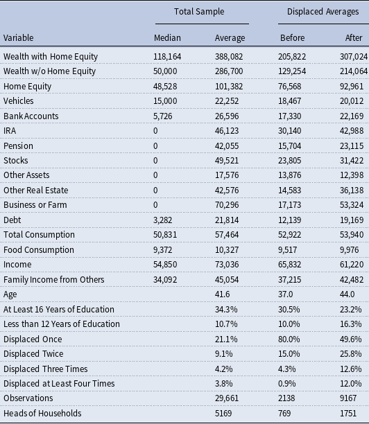
Summary statistics for these variables and others of importance are available in Table 1. These values have been adjusted with CPI-U-RS using 2017 as the base year and these values include zeros along with potentially negative values. Medians and averages are displayed for the total sample. These values for overall wealth (Wealth with Home Equity) are in line with that found in Pfeffer et al. (Reference Pfeffer, Schoeni, Kennickell and Andreski2016) that compare the PSID and the 2007 Survey of Consumer Finances. The wealth median is also in line with the more recent Survey of Consumer Finances of 2017 from Bricker et al. (Reference Bricker, Dettling, Henriques, Hsu, Jacobs, Moore, Pack, Sabelhaus, Thompson and Windle2017). However, the average is lower here and generally in the PSID as discussed in Pfeffer et al. (Reference Pfeffer, Schoeni, Kennickell and Andreski2016). Note that the averages for the components of wealth do not add up due to the missing information on IRAs noted above. Finally, the total consumption to wealth ratio aligns with Blundell et al. (Reference Blundell, Pistaferri and Saporta-Eksten2016).Footnote 8
PSID summary statistics

All the values here have been adjusted to 2017 values. Values for “Displaced” include all the observations before the event in the first column and all the observations after in the next column. See more details on the sample and these variables in Section 2 with a discussion of this table in Section 2.1.
Overall, the sample includes 1751 heads of households who have been displaced at least once along with 3418 heads that have never been displaced. This ratio of displaced workers to those that have never been displaced is similar to that of a recent published paper on displaced workers using the PSID, Krolikowski (Reference Krolikowski2018). The displaced sample has averages for before and after displacement.Footnote 9 These averages, whether they be before or after displacement, are lower than the averages in the total sample for every category listed. However, the sample of workers before displacement are younger than the total sample. Therefore, the differences between the total sample and the displaced workers before the event are not as large as the numbers suggest. The workers after displacement have more wealth than they had before since they are now much older. Looking through a few more of the notable variables show what is perhaps a surprise: debt levels for the displaced are lower although this could point to credit constraints. All types of consumption are also smaller although the gap between the total averages and the displaced averages in consumption is not as large as the gaps in wealth. Finally, education levels for heads of displaced households are different compared to the total sample with displaced workers generally having less education.Footnote 10
These summary statistics also shed light on how households are accumulating wealth. The median household has $118,164 worth of wealth with roughly half of that wealth being home equity. In fact, when calculated separately, the median home equity to wealth ratio is 0.47 with 0.57 as the average value. The median values are zero for most of the wealth components. Therefore, it seems that the households in this sample have their wealth scattered throughout different avenues. This makes it difficult to answer the question of how households end up with less wealth after displacement.
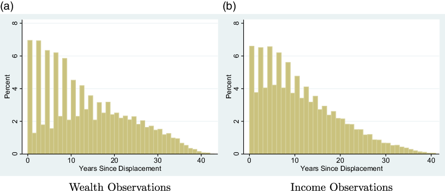
Time since displacement is also an important variable for this article but the new biennial format of the PSID makes estimating some of these years imprecise. Figure 1 provides the positive distribution on time since displacement conditional on being in this article’s samples; the width of each bar represents one year since displacement. The figure indicates that the odd values are much less common than the even values, but this is a much bigger problem for the wealth observations in Figure 1a compared to the income observations in Figure 1b. For example, in Figure 1a, 7% of the displaced wealth observations are from 2 years after displacement and 6% are from 4 years after displacement while 1% are from 1 year after displacement and 2% from 3 years after displacement. Due to the small sample size on the odd years, care must be taken when examining these as is discussed in the next section.
Observations since displacement.
These figures plot the percent density of positive time since displacement for observations from the displaced heads that are part of the wealth sample for this paper. The width of each bar represents one year since displacement. Figure 1a demonstrates the distribution of positive time since displacement for the wealth observations while Figure 1b demonstrates this for the income observations.

3. Estimation using the PSID
This article builds off the event study from Jacobson et al. (Reference Jacobson, LaLonde and Sullivan1993) and insights from Stevens (Reference Stevens1997) to compare displaced workers with their counterparts who have not been displaced below in equation (1). All the workers help determine the coefficients on the controls in an attempt to isolate the effect of displacement. Huckfeldt et al. (Reference Huckfeldt2018), Jolly (Reference Jolly2015) and Krolikowski (Reference Krolikowski2018) are recent publications that examine displaced workers with an estimation strategy similar to this. The dependent variable,
 $w_{i,t}$
, reported by an individual head of household i, takes on different values for income, wealth, wealth components, consumption, and food consumption leading to several estimations.
 \begin{equation} w_{i,t}= \sum_{m}\beta_{m}{D1}_{i,m} + \gamma_1 D2_{i} + \gamma_2 D3_{i} + \gamma_3 D4_{i} + \Theta \textbf{X}_{i,t} + \Phi\textbf{I}_{CD|HSD} + \zeta_i + y_{t} + \textbf{S} + \epsilon_{i,t}\end{equation}
Time since first displacement is indicated with a time-varying vector,
 $D1_{i,m}$
, that takes two different forms. Several studies such as Jacobson et al. (Reference Jacobson, LaLonde and Sullivan1993) and Stevens (Reference Stevens1997) find that income begins to drop before displacement and therefore this article controls for those differences up to 4 years before the event. Due to the issues mentioned earlier, time since displacement is grouped into 2-year time intervals. Specifically, the time since that displacement is estimated for m = –4 or –3, –2 or –1, 0 or 1,…, 18 or 19 and 20 plus years. For ease in reporting, an alternative for this vector groups the time since displacement into larger intervals with m = –4 or –3, –2 or –1, 0 or 1, 2 or 3, 4 to 11, and 12 plus years.
Additional displacements are estimated with time-varying indicator functions
 $D2_{i}$
,
 $D3_{i}$
, and
 $D4_{i}$
. Stevens (Reference Stevens1997) emphasizes that multiple displacements are essential for understanding the effects of displacement and therefore this article includes these controls.
 $D2_{i}$
is one if the head of the household, i, was displaced at least twice but it would be zero up until that second displacement. The same idea holds for
 $D3_{i}$
and
 $D4_{i}$
which control for being displaced at least three times and at least four times respectively.
Income along with spousal income is included in the time-varying vector (
 $\textbf{X}_{i,t}$
) because this allows the reader to see if potential differences are extraordinary. Including these income variables introduces a bias in terms of understanding the overall effect due to an involuntary displacement. However, without these controls, the changes to relative wealth and relative consumption may be due to income alone since the literature has established that income falls after displacement.Footnote 11
Additional time-varying characteristics for the heads of households (
 $\textbf{X}_{i,t}$
) includes variables for age, age squared, and age cubed along with an indicator for being currently separated from the partner, the number of children in the household, and several dummy variables representing various types of pensions or employer-based retirement plans the head or spouse may have.Footnote 12 The age terms are interacted with whether the worker has at least 16 years of education or has less than 12 years of education in (
 $\textbf{I}_{CD|HSD}$
) because income patterns vary on education and the summary statistics in Section 2.1 indicate differences in education levels for displaced workers. Therefore, the results compare the dependant variable for the displaced head to other heads of similar education. Controls are included for the quantity of household members since this affects the levels of consumption and wealth. Types of pensions and/or retirement plans can also affect wealth accumulation which explains their dummy variable controls.
Finally, all estimations include three different types of fixed effects. Individual fixed effects for the head of the household (
 $\zeta_i$
) are included in an attempt to control their idiosyncracies. Fixed effects for the state of residence (
 $\textbf{S}$
) are included to help control for local conditions, like housing values, that vary across the USA.Footnote 13 Annual fixed effects (
 $y_t$
) help with changing values of wealth due to their respective markets. These fixed effects are also useful for controlling any systematic differences in the PSID that are unknown to the author.
3.1 Empirical results from the PSID
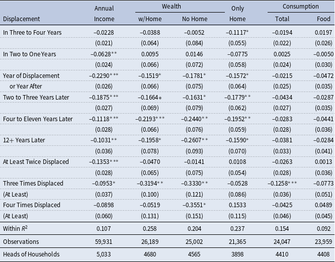
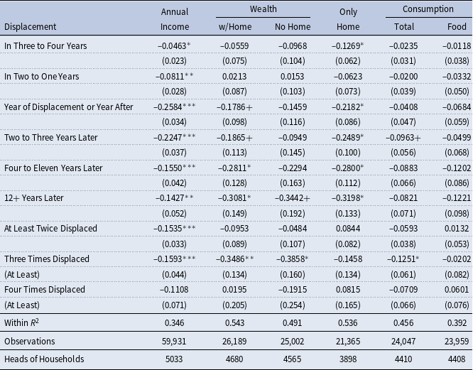
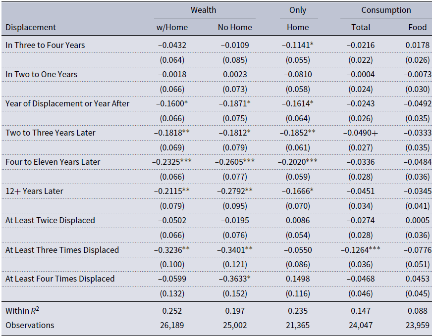
Table 2 presents the main findings from this study with the format of this table followed throughout the empirical results. The first row indicates the log transformed dependent variables used in the estimation of equation (1). The first column indicates time since displacement and indicators for multiple displacements. The table reports the values of the coefficients for these displacement indicators without parentheses and the numbers with parentheses are the standard errors clustered for each head of household. Observations can vary due to the log transformation dropping nonpositive values or due to the changing availability of information noted in Section 2. The individual heads of households vary because every estimation requires that each individual have at least two observations.
Effects of displacement on income, wealth, and consumption

Significance levels: + : 10% * : 5% * * : 1% * * * : 0.1%
Note: This table displays the results of equation (1) with m = −4 or −3,..., 4 to 11 and
 ${D1}_{i,12p}$
controlling for time-varying individual characteristics including composition of household, annual fixed effects, state fixed effects, and individual fixed effects. Income is a control for the wealth and consumption estimations. The wealth estimates control for the holdings of different types of pensions. See Section 3 for more details on this strategy. The first row indicates the dependent variables with the log transformation. The three wealth estimates include wealth with home equity (w/Home), wealth excluding home equity (No Home), and only home equity (Only Home). The values without parentheses are the coefficients for the independent variables listed in the first column which indicate time since displacement and whether the worker has been displaced multiple times. The numbers in parentheses are the standard errors clustered at the individual level.
When workers experience an involuntary displacement, income falls immediately, and their income remains lower than their peers’ income. This is noted in the literature from the introduction and is shown again in Table 2 to put the other results into context. Specifically, the income column of this table shows the results of estimating equation (1) on log annual income. Income is 20% (
 $-0.2$
=
 $e^{-.229}-1$
) lower for displaced workers compared to their peers upon the first two years of displacement and income is still 10% lower 12 plus years later.Footnote 14
Table 2 makes clear that when the head of a household experiences an involuntary displacement, wealth is lower than the head’s peers and that fall in wealth displays little to no recovery.Footnote 15 Specifically, total wealth is 14% lower in the year or in the year after the first displacement and is 15–20% lower than expected in all the following years.Footnote 16 Housing wealth falls in similar magnitudes although this fall begins before displacement. However, wealth that excludes housing falls by 16% upon displacement with this fall increasing to 23% when the first displacement occurred at least 12 years prior.
The value of wealth should not be driving these results. The estimates in Table 2 include time dummy variables which should capture national changes in several of the assets. While home equity is more local, wealth that excludes this is still much lower for displaced households suggesting that local conditions are also not the primary source for these results.
The literature in the introduction indicated wealth reductions in the 8% to 13% range. Table 2 demonstrates larger magnitudes but given that previous research involved older workers from the HRS, the deviations for this difference are not surprising. Older workers have more wealth and therefore their percentage decreases should be smaller. Additionally, since older workers are closer to retirement, there is less time for the workers to fall further behind their peers.
The results in Table 2 indicate that consumption falls upon displacement but that this fall is small to non-existent. The estimates range from a 2 to 4% decrease for overall consumption but the results are not statistically different from zero. The results on food consumption are similar with the consumption of food falling 3–4% but again these results have relatively large standard errors. The food consumption results are different from the results found in Stephens Jr (Reference Stephens2001) where food consumption falls 9–11% after displacement with much more precision (smaller standard errors). These differences are further explored in the appendix Section C.Footnote 17
The fact that consumption does not fall much after an involuntary displacement is in line with consumption smoothing theory. The idea that individuals and households attempt to keep their consumption steady (consumption smooth) has a long history as Meghir and Pistaferri (Reference Meghir and Pistaferri2011) discuss in their chapter from the Handbook of Labor. More recent work in this area includes Blundell et al. (Reference Blundell, Pistaferri and Saporta-Eksten2016) who use a flexible life cycle model calibrated to the PSID to show the various avenues used to insure consumption streams within a family. That paper demonstrates the various consumption changes with respect to changes in wages. The two elasticities, which capture these ratios of changes, have different signs indicating that the overall difference in consumption may not be significantly different from zero. Sullivan (Reference Sullivan2008) examines the various impacts of unemployment on consumption for those with assets versus those without assets using the SIPP and the PSID. That paper finds that those with assets do not cut their consumption as much as those without assets. A heavy majority of the sample in Table 2 has assets and therefore, these results do not run counter to those in Sullivan (Reference Sullivan2008).
3.2 Wealth components
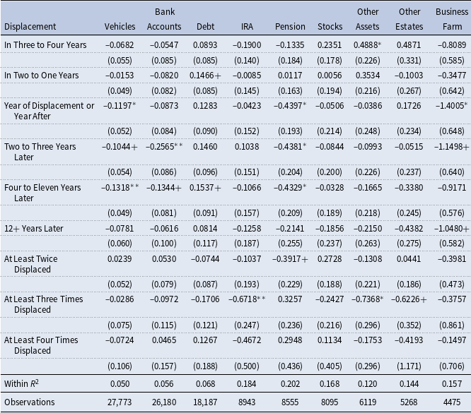
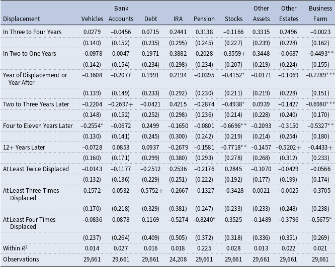
Table 3 also emphasizes the main point of this article: when displacement occurs for the household, wealth, no matter the type, falls relative to other similarly educated households. This table presents the results of estimating equation (1) from Section 3 with the dependent variable being the individual components of wealth after a log transformation. Almost all of the estimates in this table indicate a loss in wealth. For example, the last column of this table indicates that the value of a farm or business is 75% (
 $-0.75$
=
 $e^{-1.4}-1$
) lower than expected for households that have the head displaced.
Effects of Displacement on Wealth Components

Significance levels: + : 10% * : 5% * * : 1% * * * : 0.1%
Note: This table displays the results of equation (1) with m = −4 or −3,..., 4 to 11 and
 ${D1}_{i,12p}$
controlling for time-varying individual characteristics including all household income, composition of household, annual fixed effects, state fixed effects, and individual fixed effects. See Section 3 for more details. The first row indicates the dependent variables. “Bank Accounts” indicate the sum of checking and savings accounts, “IRA” indicates the value of private annuities and IRAs, “Other Assets” indicate the value of assets such as bonds, life insurance, trusts, estates and collections, “Other Estates” indicates the value of nonprimary real estate; see Section 2 for more details on these components. The values without parentheses are the coefficients for the independent variables listed in the first column which indicate time since displacement and whether the worker has been displaced multiple times. The numbers in parentheses are the standard errors clustered at the individual level.
The interpretation of these results in Table 3 must be done with care since most of these wealth components have a median value of $0 as shown in Table 1. The estimation strategy in this article is to compare workers that have been displaced to workers that have not been displaced and have non-zero values since these results have a natural log transformation.Footnote 18 The first column of results in Table 3, which is for vehicles, has 27,773 observations or 94% of the total from this paper’s sample but the last column of results for the value of a business or farm indicates 4475 observations or 15% of the total from this paper’s sample. Therefore, when stating that the value of the farm or business is 75% lower than expected, this is based on the individual fixed effect and the non-displaced workers of a similar education who own a farm or business with a positive value.
3.3 Robustness – individual time trends
This section provides a robustness check of Table 2 by examining those results with an individual linear time trend. This time trend goes one step further than the individual fixed effect to examine whether the specific individuals not only have different levels but also different rates of accumulation. This is helpful if displaced workers happen to have different rates of wealth accumulation compared to their counterparts. Specifically, this robustness check is simply estimating equation (1) with an additional term,
 $\lambda_i t$
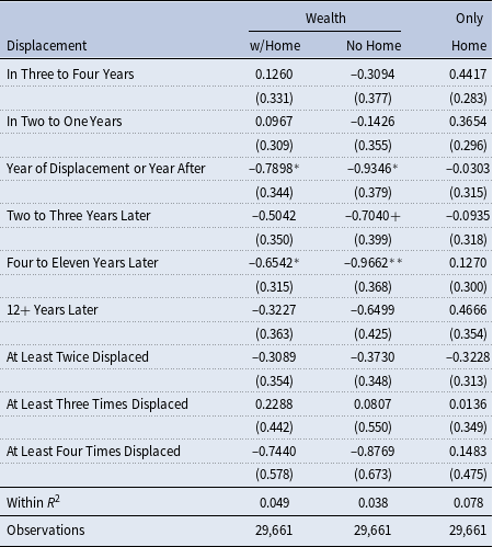
. The results are in Table 4 and indicate that the main results still hold; wealth drops upon displacement and this fall in wealth has a lasting impact. This holds whether the wealth includes home equity or not. The results for consumption are also largely unchanged although the point estimates display larger magnitudes. Section D of the appendix contains more robustness results including estimates containing zeros and negative values using the inverse hyperbolic sine transformation along with a note on the results without any transformation.
Robustness – Effects of displacement with individual time trends

Significance levels: + : 10% * : 5% * * : 1% * * * : 0.1%
Note: This table displays the results of equation (1) with m = −4 or −3,..., 4 to 11 and
 ${D1}_{i,12p}$
controlling for time-varying individual characteristics including composition of household, annual fixed effects, state fixed effects, individual fixed effects, and individual time trends. Income is a control for the wealth and consumption estimations. The wealth estimates control for the holdings of different types of pensions. See Sections 3 and 3.3 for more details. The first row indicates the dependent variables with the log transformation. The three wealth estimates include wealth with home equity (w/Home), wealth excluding home equity (No Home), and only home equity (Only Home). The values without parentheses are the coefficients for the independent variables listed in the first column which indicate time since displacement and whether the worker has been displaced multiple times. The numbers in parentheses are the standard errors clustered at the individual level.
4. Theory
4.1 Model
A general life cycle model is useful because it provides the framework on what should be expected regarding wealth and consumption after displacement. Specifically, it helps to answer whether to expect workers to cut back more on consumption or wealth. This article compares the aforementioned findings from the PSID to the life cycle model available in Carroll (Reference Carroll2012) which is similar to that in Cagetti (Reference Cagetti2003), Carroll et al. (Reference Carroll, Hall and Zeldes1992) and Carroll (Reference Carroll1997). The model is of partial equilibrium where the dynamic problem for the agent is one of choosing consumption and hence savings for wealth. This choice is made to maximize utility for the rest of one’s life based on income that is subject to life cycle growth along with uninsurable shocks. Specifically, the maximization problem for each agent is as follows:
 \begin{equation*}\max \left\{ u(C_{t})+E_{t}\left[\sum_{s=t+1}^{T} {\delta}^{s-t}\left( \Pi_{i=t+1}^{s}{\beta}_{i}\pi_{i}\right) u(C_{s}) \right]\right\}\end{equation*}
subject to
 \begin{eqnarray*} C_{s}+A_{s} &=&\hat{R}A_{s-1}+P_{s}\Theta_{s} \space \forall s\\ P_{s} &=&G_{s}P_{s-1}N_{s}\end{eqnarray*}
Utility in time period t is derived from consumption (
 $C_{t}$
) along with the expected utility going forward with two discount factors. The time invariant discount factor (
 $\delta$
) makes up the first with the second being a time-variant discount factor (
 $\beta_{s}$
) between ages s and
 $s-1$
used to reflect changes in spending over an agent’s lifetime. Agents also face the possibility of death later in life with
 $\pi_{s}$
being the probability of living until age s given living until age
 $s-1$
. The choice for consumption indicates how much is saved (
 $A_{s}$
) in time s which provides a constant gross interest rate (
 $\hat{R}$
). The right-hand side of the budget constraint also includes permanent income (
 $P_{s}$
) which is exposed to a temporary shock (
 $\Theta_{s}$
) that can take the value of zero with probability p but otherwise follows a log normal distribution. Permanent income grows at a rate
 $G_{s}$
between age
 $s-1$
and s while being exposed to another shock (
 $N_{s}$
) with a log normal distribution detailed below:
 \begin{eqnarray*} \Theta_s &=& 0 \text{ with probability } p \\ &=& Z_s/(1-p) \text{ with probability }(1-p) \\ \log Z_s &\thicksim& \mathcal{N}(-\sigma _{\Theta }^{2}/2,\sigma_{\Theta}^{2}) \\ \log N_s &\thicksim& \mathcal{N}(-\sigma_{N}^{2}/2,\sigma _{N}^{2})\end{eqnarray*}
Shocks to income create displacements in the model. Displacements for the model depend on the severity (
 $\gamma$
) of the negative shock. Therefore, this article defines a displacement as occurring in the model when either of the following holds:
 \begin{eqnarray*} N_{s} &<& 1 - \gamma_N * \sigma_{N} \\ \Theta_s &<& 1 - \gamma_{\Theta} * \sigma_{\Theta}\end{eqnarray*}
Displacements in the model depend on both types of shocks. The model needs displacement from temporary shocks to replicate the fact that several displaced workers recover. If permanent shocks are the only target, there is not enough recovery. If temporary shocks are the only target, the average worker recovers immediately. Thus, the displaced sample needs to be a mix of those that have experienced permanent shocks and those that have experienced temporary shocks. Alternative possibilities of defining displacements for this model are discussed in Section 4.6.
A key reason for using this model is its simplicity with the presence of permanent shocks to income. Its simplicity makes calibrating to new variables easier while previous research demonstrates its use for understanding wealth. The permanent shocks to income are crucial since most involuntary job displacement is accompanied by permanent decreases to income as noted in the introduction and found in Table 2. However, this article does not attempt to explain the nature of these decreases as in Jarosch (Reference Jarosch2015), Krolikowski (Reference Krolikowski2017), or Michaud (Reference Michaud2015). Rather, these shocks are a mechanical part of this framework.
4.2 Simulation
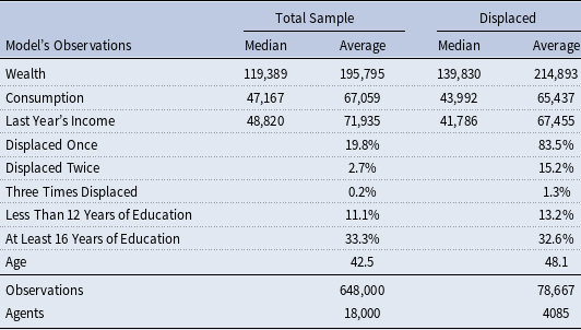
The simulated data on consumption, income, and displacement comes from using the model to generate panel data for the three different types of workers identified in Cagetti (Reference Cagetti2003): those with less than 12 years of education, those with 12–15 years of education, and those with at least 16 years of education. These agents are capable of living up to 90 years old. For purposes of this article, the simulated data is collected on agents aged 25–60 to match the age groups from the empirical work done with the PSID in this paper (Table 2). Therefore, the model is simulated three times to produce a total of 18,000 workers with 648,000 observations where the proportions of the workers roughly reflect those from this paper’s sample. Specifically, the code from Carroll (Reference Carroll2012) solves the model above for one type of worker with variables normalized as a percentage of permanent income (
 $P_{s}$
). Creating permanent income variables that scale the original variables result in the simulated data.
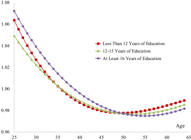
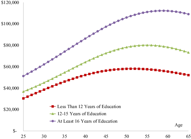
Since this model is closely related to the model in Cagetti (Reference Cagetti2003), a handful of the model’s parameters come from that paper. The values for the probability of staying in the labor force (
 $\pi$
) are equal to one for these 25–60-year-old agents. The real return to saving is set constant at 3% (
 $\hat{R}=1.03$
). The values for the time-varying discount factor (
 $\beta$
) correspond to each type of agent and are summarized in Figure E.1 of the Appendix. The values for the growth rate of income (G) together with each type of worker’s starting permanent income (
 $P_{25}$
) are summarized in Figure E.2 of the Appendix.
The temporary shocks along with the permanent shocks follow a log normal distribution with the shocks having a mean of one and standard deviations calculated from the PSID. The income process for the three different types of workers is estimated using the first differences in log income following Heathcote et al. (Reference Heathcote, Perri and Violante2010) which uses heads of households that have worked more than 260 hours with a calculated hourly rate greater than $2. The results of this approach are much closer to that of Carroll et al. (Reference Carroll, Hall and Zeldes1992) which is used in Carroll (Reference Carroll1997) as opposed to using moments in log income levels. The temporary shock to income (
 $\Theta$
) can result in zero income with probability
 $p=0.5$
% for all worker types; this number comes from this paper’s PSID sample and is also used in Carroll (Reference Carroll1997). The distribution of these shocks is reported in Table 5.
Model parameters

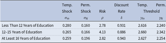
Note: This table summarizes all the parameters used in the model. The first two columns of parameters are found using first differences in log income following Heathcote et al. (Reference Heathcote, Perri and Violante2010). The next two columns are found using simulated method of moments where the targets and the model’s performance are found in Table E.1. The last two columns determine the thresholds for what creates a displacement in the model. These are found using another round of simulated method of moments with the targets and performance in Table E.2. See more details in Section 4.2.
Table 5 provides the rest of the calculated parameters for the model. The functional form for utility is one of constant relative risk aversion (
 $u(C_s)= C_{s}^{1-\rho}/(1-\rho)$
) where the risk parameter (
 $\rho$
) and the time invariant discount factor (
 $\delta$
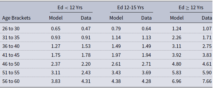
) for each type of worker is found using the method of simulated moments. This process is used for each type of worker to approximate the median wealth to income ratios for seven age groups (26–30, 31–35, etc.) from the 1992 through the 2007 waves of the Survey of Consumer Finances with each moment having an equal weight following the procedure in Carroll (Reference Carroll2012). As explained in Carroll (Reference Carroll2012), the median wealth to income ratio is the target since this model is not designed for the high concentration levels of the most wealthy. The wealth medians and averages for the PSID sample in this study are also more representative of those outside these high concentration levels as noted in Section 2.1. The targets and the model’s performance are available in Table E.1 of the appendix.
The severity of the shocks denoted with
 $\gamma_N$
and
 $\gamma_{\Theta}$
are chosen to target the income distribution for displaced workers using a second round of simulated method of moments after the risk parameter (
 $\rho$
) and the time invariant discount factor (
 $\delta$
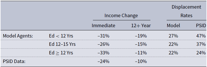
) are determined. Specifically, the targets come from the following differences in income found in Table 2: 2–3 years later, 4–11 years later, and 12 plus years later. The targets also include the proportion of each worker type that experiences a displacement and the peak fall in income after displacement. It is important to use the peak fall in income because when displacement occurs in the model, income takes a large fall. The peak fall in income comes 1 year after displacement when income falls by 24%.Footnote 19 Each of the targets has an equal weight resulting in the values for each
 $\gamma$
in Table 5. The targets and the model’s performance on these dimensions are listed in Table E.2 of the appendix. However, the calibration strategy is not driving the results; Section 4.6 provides more information on alternative strategies for calibration and their issues.
4.3 Model summary statistics
The data generated by the model is summarized with the model’s summary statistics in Table 6. The model does a decent job with generating displacements correctly although there is one important thing to keep in mind when examining these numbers: displaced agents in the model are older than the displaced workers in the PSID data and the displaced agents are much older than the total sample from the model. This explains why the displaced agents in the model have more wealth than the total sample; they are older. The model also has a smaller percentage of agents being displaced.
Summary statistics from the model

All the values here have been adjusted to 2017 values. See Section 4.1 for more details on the model and the calibration. Values for “Displaced” come from all the observations after displacement.
4.4 Estimation using the model
The model, calibrated to generate a permanent decrease in income like that in the data, is now used to examine wealth and consumption after an event like displacement. Equation (1) again considers dependent variables (
 $w_{i,t}$
) to be income, wealth, and consumption. The setup and estimation for the model’s data is nearly the same as the estimation using the PSID. Because the model’s data is more abundant, time since the first displacement is estimated annually. Several controls like state and year fixed effects are unnecessary for this simulation data but for comparison to the empirical results, the individual fixed effect (
 $\zeta_i$
) is included. These individual fixed effects also help correct for the fact that the average values for wealth and consumption differ in the PSID data compared to the generated data from the model.
4.5 Estimation results from the model
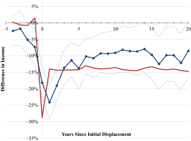
Figure 2 demonstrates the drop in income experienced by agents in the model in direct comparison to the heads of households from the PSID. The solid line without markers comes from the
 $\beta$
coefficients on time since displacement for income based on equation (1) from the model. As shown, these agents experience a slightly larger drop in income with the fall being even worse every year after three years since displacement. When summing the decreases across the first 19 years of displacement, this costs the displaced agents 42% more income relative to the heads from the PSID.
Income differences due to displacement.
The solid line without markers indicates the difference in income which come from
 $e^{\beta}-1$
where the
 $\beta$
’s come from equation (1) for the model and the solid line with square markers identify these values from the PSID data. The thin dashed lines are the 95% confidence intervals for the estimations from the PSID. The model’s extension with habit formation has the identical results as the solid line without markers.

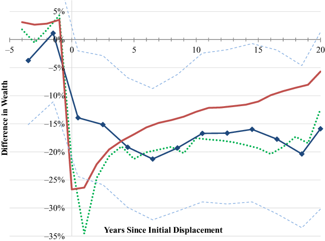
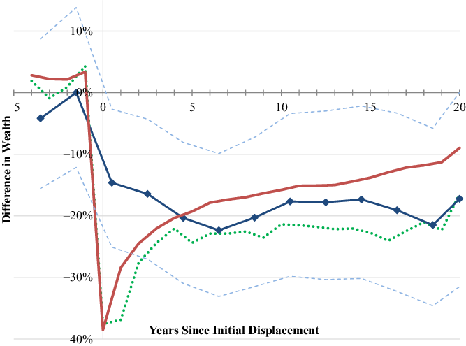
Figure 3 depicts that displaced agents in the model experience a large loss in wealth, but they recover contrary to what is found in the PSID. The line without markers indicates the difference in agents’ wealth that comes from the values for the
 $\beta$
coefficients from equation (1) when time since displacement is measured annually. In the year of displacement, the agents have 27% less wealth compared to their counterparts from the model that are of equal age and education. However, wealth continues to increase relatively as the agents rebuild their wealth to buffer income shocks. As shown, this is much different than the results from the PSID even though the calibration has a fall in income being worse for those in the model.
Wealth differences due to displacement.
The solid line without markers indicates the difference in wealth which come from
 $e^{\beta}-1$
where the
 $\beta$
’s originate from equation (1) for the model and the solid line with square markers identify these values from the PSID data. The thin dashed lines are the 95% confidence intervals for the estimations from the PSID. The dotted lines provide these values for the model’s extension which include habit formation.

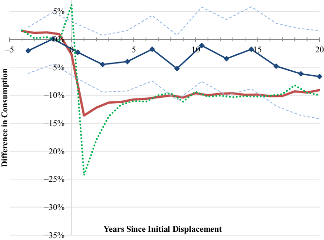
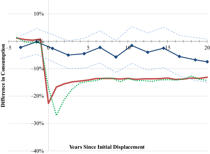
Figure 4 depicts consumption after displacement for agents in the model compared to the PSID, which is an important cause of the different wealth experiences. The agents in the model decrease their consumption by 14% in the year after displacement and this decrease in consumption is still at 9% 20 years after displacement. Comparatively, households in the PSID are not changing their consumption in this fashion although their decreases in consumption are increasing in magnitude over time. In the year of displacement, the fall in consumption for agents in the model appears small due to income as an independent variable for these estimations. In other words, consumption relative to income does not fall much in the year of displacement because income is so low for displaced workers in the model. This also occurs on a smaller scale for the PSID.
Consumption differences due to displacement.
The solid line without markers indicates the difference in consumption which come from
 $e^{\beta}-1$
where the
 $\beta$
’s originate from equation (1) for the model and the solid line with square markers identify these values from the PSID data. The thin dashed lines are the 95% confidence intervals for the estimations from the PSID. The dotted lines provide these values for the model’s extension which include habit formation.

4.6 Alternative calibration strategies
This section considers alternative strategies for defining a displacement in the model. Simply relying on the permanent component of the income process is intuitive since the results in Figure 2 seem to indicate a permanent fall in income. Following a similar method of moments of targeting the income scar along with the displacement ratios leads to permanent falls in income, wealth, and consumption but the magnitudes are much too large, and the model generates too many displacements. Specifically, this strategy leads to 52% of the agents experiencing a displacement, income falling 40% which leads to consumption falling 22%. This performs poorly because there is too little recovery in the model when displacements are only based on permanent shocks. While several workers in the PSID experience a permanent fall in annual income, several others recover which is why both types of shocks are needed.
Another alternative strategy is to only target the initial fall in income and the fall in income 12 years after displacement with the requirement that the lasting fall in income is no more severe than that found in the data. This strategy also requires that the displaced population make up no more than 50% of the population although the results are similar if including the proportion of the population displaced as a target; this 50% threshold gives the parameters their best chance of matching the fall in income. This strategy may be enticing since the current targets lead to an income scar that is worse than that in the data as is clear in Figure 2. However, this strategy leads to wealth recovering even faster. Since wealth recovers faster, the fall in consumption is smaller yet agents in the model still cut consumption by much more than the households in the PSID.
In estimating these displacement parameters (
 $\gamma$
), the estimation strategy either needs to target the proportion of displaced workers or there needs to be a threshold for the percentage of workers displaced. Otherwise,
 $\gamma$
’s are found which create too much displacement. The interpretation of the results from estimating equation (1) would then change because the non-displaced population would be small.
4.7 Extending the general model with habits
The general model used thus far follows the literature to show that involuntary job displacement causes a permanent fall in income but the agents drastically change their consumption contrary to the findings from the PSID. Therefore, respondents in the PSID are better at consumption smoothing which may be due to habit formation. In other words, households in the PSID may be accustomed to a certain lifestyle and may be unwilling to change their spending habits unless it is absolutely necessary. For example, previous work uses habit formation mechanisms to study a wide range of issues including the equity premium [Campbell and Cochrane (Reference Campbell and Cochrane1999), among others], income and consumption aggregates [Jawadi and Leoni (Reference Jawadi and Leoni2012), among others], growth and fertility [Schäfer and Valente (Reference Schäfer and Valente2011)], and labor supply with growth dynamics [Gómez (Reference Gómez2015) among others].Footnote 20
Perhaps, the easiest way to add habit formation to the general model above is to simply consider utility to be based on the difference in consumption rather than the consumption itself. Formally, consider the following utility function for time period s:
 \begin{equation*}u(C_s)= \frac{(C_{s}-\theta C_{s-1})^{1-\rho}}{(1-\rho)}\end{equation*}
This utility function is one commonly used in the literature on habit formation, but it introduces an unknown variable
 $\theta$
which indicates the importance of last period’s consumption on utility. This parameter can take a value from zero to one with a value of zero reducing utility to the function used earlier in the paper. A value of one for
 $\theta$
indicates that utility does not depend on the level of consumption but only on how consumption today compares to consumption in the past.
This article targets the long-lasting scars to consumption and wealth to estimate the value of this
 $\theta$
parameter by using the same parameterizations and the same agents with the same income and income shocks used in the general model but simply adjusting
 $\theta$
to essentially minimize the gap between the two solid lines in Figures 3 and 4. Specifically, consider
 $\beta_{m}$
from equation (1) for the PSID on wealth as
 $\beta_{w,m}$
and these coefficients on consumption as
 $\beta_{c,m}$
. For the simulation data, which now vary with different values of
 $\theta$
, consider the same coefficients denoted as
 $\hat{\beta}(\theta)_{w,m}$
and
 $\hat{\beta}(\theta)_{c,m}$
for the estimations with wealth and consumption, respectively. Thus,
 $\theta=0.73$
is found by solving the following:
 \begin{equation*}\min_{\theta} \sum_{m = -4}^{20p}\left(\beta_{w,m} - \hat{\beta}(\theta)_{w,m}\right)^2 + \left(\beta_{c,m} - \hat{\beta}(\theta)_{c,m}\right)^2\end{equation*}
This parameter on the importance of past consumption,
 $\theta$
, has a wide range of estimated values in the literature. In fact, Deaton (Reference Deaton1986) has nearly the same value on this parameter with it equal to 0.78. A similar value of 0.80 is found in Constantinides (Reference Constantinides1990) who uses the model for understanding the equity premium puzzle. On the higher end, Carroll and Weil (Reference Carroll and Weil1994) find that their value of the parameter must be 0.95 for their model to reproduce high savings with large levels of income growth. On the lower end, Dynan (Reference Dynan2000) has several estimated values for this parameter using food consumption from the 1968 to 1987 waves of the PSID. Most of the values in Dynan (Reference Dynan2000) are less than 0.15 but interestingly, the largest value of 0.66 is found only when using job displacement as the instrument. Additionally, Dynan (Reference Dynan2000) provides a discussion on how this
 $\theta$
parameter can have such large variation based on different strategies of estimation.
This extension of the model with habits provides an improvement with coefficients closer to those from PSID compared to the general model. However, this improvement comes exclusively from wealth. In fact, the coefficients on wealth are 30% closer to that in the data with the average fall in wealth being 16% in the model’s extension compared to the average 12% fall in wealth for the general model. (Recall that the average fall in wealth for the PSID is 15%.) This difference is visible in Figure 3 where the changes in wealth with habit formation are represented with the dotted line. As is clear in the figure, the model’s extension has a larger fall in wealth upon displacement compared to the general model which is already a larger fall than that in the data and is represented with the markered line.
The reason for the larger fall in wealth is clearer when examining the changes in consumption represented with the dotted lines in Figure 4. First, it appears that consumption increases upon displacement, but this is misleading because consumption actually falls by 17% on average for the agents upon displacement. However, recall from Figure 2 that income falls by nearly 30% for these agents. For this reason, consumption relative to income rises which explains the small jump in the figure at the time of the event.Footnote 21 In the year after what has been defined as the model’s displacement, consumption makes an even larger fall than the general model due to the larger fall in wealth. After four periods, the general model and the extension are nearly the same with both lines indicating a long-term fall of about 10% in consumption. This also needs some context because the displaced agents consume more in the model with habits than the agents in the general model; but all agents in the habits model consume more than in the general one used earlier. This explains why wealth does not recover since both models have the exact same incomes. Overall, the model’s extension performs a little worse with the average consumption marker indicating a 9% fall compared to the average 8% fall in consumption from earlier which are both worse than the data’s 3% fall.
4.8 Wealth at death
The results in this article suggest that wealth for displaced workers would be lower upon death if wealth continues its trajectory of non-recovery. Indeed, this lack of recovery persists when broadening the data to include older heads of households from the PSID. When relaxing the requirement that heads of households must be no older than 60 years of age, the figure for changes in wealth has a lasting and statistically significant fall going out to 30 years from the time of displacement. Specifically, the wealth for displaced heads of households from the PSID is 19% lower than their nondisplaced peers when it has been 30–31 years since displacement.
The key result for the extended model with habit formation is that the long run results for wealth are similar to those in the PSID. This is clear in Figure 3. Like the PSID, extending the model to include older agents results in wealth that also does not recover. The wealth for displaced agents when it has been at least 30 periods since the event is 17% lower than their nondisplaced peers.
The extended model provides insight for what we should expect from bequests for displaced workers. Although the PSID collects information on gifts and inheritances, this information is for the recipients rather than for those that provide the bequest. However, wealth held by agents at death provide intuition on what to expect in other datasets. Recall that older agents of age s die at probability
 $1-\pi_{s}$
as noted in the model’s description above. In the model’s extension, wealth at death is 27% lower for those that have experienced a displacement compared to the agents that have not. Therefore, bequests for displaced workers should be much lower than the bequests for nondisplaced workers and this model provides an idea on the magnitude to expect.
5. Conclusion
The main purpose of this article is to investigate the level of wealth over time for displaced workers. Only recently has there been enough data to perform this type of exercise on wealth which contributes to this paper’s novelty. Households with a displaced worker present have 18% less wealth when including home equity and 23% less wealth when ignoring home equity 12 years after displacement relative to their peers. This is a larger fall in wealth compared to previous findings. This article also shows that to understand this effect on wealth, consumption is an important driver. Contrary to previous findings, in the newer PSID data, consumption demonstrates no significant fall after displacement with this same pattern holding true for food consumption. This result on consumption is also novel since there has been little work done like this with the newer measures of consumption in the PSID. These newer measures demonstrate a smaller fall than previously found.
A general life cycle model calibrated to the PSID with permanent decreases in income after displacement also demonstrates a large drop in wealth, but in contrast to the data it illustrates recovery. The general model also suggests a larger fall in consumption compared to the PSID. However, extending the model to include habit formation improves the model’s overall fit on wealth but most importantly, the model delivers similar long run losses to wealth. Therefore, this article shows that the displaced agents in the model have 27% less wealth compared to nondisplaced agents at death. These results from the model are informative for future research on bequests but ultimately, the findings throughout the article provide several avenues for future work. The empirical results together with the procedure used for assessing the theory here will benefit this future research.
Acknowledgments
Thank you to Bruce Fallick, Andy Glover, Lockwood Reynolds, Anne Winkler, anonymous referees, editors, and participants of the following for their helpful comments: Kent State Economics Seminar Series, Midwest Macroeconomic Meetings, Society for the Advancement of Economic Theory Conference, Southern Economic Association Meetings, Cleveland State Economics Seminar Series, and the SOLE Session of the Midwest Economics Association.
A. Appendix
Effects of displacement on wealth and consumption without income controls

Significance levels: + : 10% * : 5% * * : 1% * * * : 0.1%
Note: This table displays the results of equation (1) with m = −4 or −3,..., 4 to 11 and
 ${D1}_{i,12p}$
controlling for time-varying individual characteristics including composition of household, annual fixed effects, state fixed effects, and individual fixed effects. See section 3 for more details on this strategy. The first row indicates the dependent variables with the log transformation. The three wealth estimates include wealth with home equity (w/Home), wealth excluding home equity (No Home), and only home equity (Only Home). The values without parentheses are the coefficients for the independent variables listed in the first column which indicate time since displacement and whether the worker has been displaced multiple times. The numbers in parentheses are the standard errors clustered at the individual level.
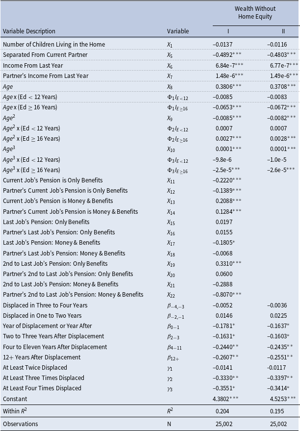
Control variables with and without controlling for pension

Note: This table displays most of the control variables from the results in Table 2 for total log wealth excluding home equity with controls for pension type in column I and without controlling for pension type in column II. Additional controls include annual fixed effects, state fixed effects, and individual fixed effects.
Wealth differences due to displacement without income controls.
These differences in wealth come from
 $e^{\beta}-1$
where the
 $\beta$
’s originate from equation (1) without controlling for income. The solid line without markers indicate these values for the model and the solid line with square markers identify these values from the PSID data. The thin dashed lines are the 95% confidence intervals for the estimations from the PSID. The dotted lines provide these values for the model’s extension which include habit formation.

Consumption differences due to displacement without income controls.
These differences in consumption come from
 $e^{\beta}-1$
where the
 $\beta$
’s originate from equation (1) without controlling for income. The solid line without markers indicate these values for the model and the solid line with square markers identify these values from the PSID data. The thin dashed lines are the 95% confidence intervals for the estimations from the PSID. The dotted lines provide these values for the model’s extension which include habit formation.

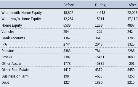
B. Changes in wealth
Average annual changes in wealth and their components for displaced workers are in Table B.1. The first column reports wealth variables and the next column indicates how that variable changes on average in between the two years for which the head reported its wealth and components. Before displacement, overall wealth increases annually by 18,802. In the year of displacement or the year after, overall wealth drops by 4613. When calculated separately, the average wealth for households that are not displaced but that will be displaced is 205,822. If a worker with the average wealth of $205,822 is displaced, their new level of wealth would be 201,209 instead of the 224,625 that would have occurred with the average growth of 18,802. This represents a 10% difference in wealth. This is lower than the 14% difference in wealth reported from Table 2 because these averages do not account for the fact that households accumulate more wealth as they age along with the other control variables from equation (1).
Table B.1 also points out which components fall the most in value on average. Here, the average fall is biggest in the value of stocks and other assets with these values dropping by roughly $5000 on average. Home equity, the overall value of all bank accounts and IRAs still rise but the rise is smaller than before displacement. These values are helpful in understanding how displaced heads of households respond to their displacement event.
Change in variables for displaced households

Note: This table provides the average difference in the variables listed in the first column for the households whose head is displaced. The second column provides these changes before displacement, the next column is in the year or the year after displacement, and the last column provides these changes after displacement.
C. Food consumption differences
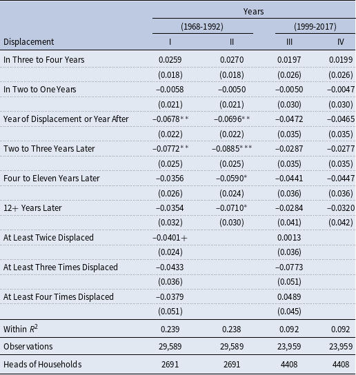
This section briefly examines the differences in the food consumption results from this paper compared to Stephens Jr (Reference Stephens2001). Table C.1 displays the results of equation (1) with m = −4 or −3,…, 4 to 11 and
 ${D1}_{i,12p}$
with the first two columns (I & II) having the log transformed food consumption data from 1968 through 1992 excluding 1973, 1988 and 1989 since this data was not collected in those waves. 1968 through 1992 is the timeframe and the variables used in Stephens Jr (Reference Stephens2001). The last two columns (III & IV) use the log transformed food consumption data from this paper which covers every two years starting in 1999 and ending in 2017. The estimations are the same as in equation (1) of Section 3 except that there is no pension controls since there is no pension information for any year before 1999 other than 1984. Columns II and IV are more similar to Stephens Jr (Reference Stephens2001) in that they do not control for multiple displacements. Otherwise, the tables have the same control variables discussed in Section 3.
The sample construction in this paper compared to Stephens Jr (Reference Stephens2001) is also slightly different. The heads of households in this table all have at least two observations like the empirical results elsewhere in this paper. The first two columns have more observations since they cover more years of data but they have fewer individuals since the sample for this paper steadily grows every year until 2009 before it makes a small fall and plateaus.Footnote 22 The heads for the sample in Table C.1 all have one wealth observation although the results are not statistically different if ignoring this requirement. Stephens Jr (Reference Stephens2001) requires three consecutive observations for each head and if a head has missing information, data from the head’s household are no longer included in the estimations going forward for that paper.Footnote 23
Effects of displacement on food consumption

Significance levels: + : 10% * : 5% * * : 1% * * * : 0.1%
Note: This table displays the results of equation (1) with m = −4 or −3,..., 4 to 11 and
 ${D1}_{i,12p}$
controlling for time-varying individual characteristics including all household income, composition of household, annual fixed effects, state fixed effects, and individual fixed effects. See Section 3 for more details on this strategy. The dependent variables are the log transformation of consumption from two different time periods. The values without parentheses are the coefficients for the independent variables listed in the first column which indicate time since displacement and whether the worker has been displaced multiple times. Columns II and IV do not control for multiple displacements. The numbers in parentheses are the standard errors clustered at the individual level.
The results differ when comparing the older data in columns I & II to the newer data in columns III & IV of Table C.1. The earlier data with the results in column I and II demonstrates a fall in consumption for the first three years after displacement. Column I, which controls for multiple displacements, demonstrates some recovery in consumption spending by household. Column II, which does not control for multiple displacements, does not demonstrate a recovery in food consumption spending which is more similar to the results in Stephens Jr (Reference Stephens2001). Therefore, it seems that the lasting impact on food consumption spending found in Stephens Jr (Reference Stephens2001) is due to multiple displacements which is similar to the emphasis in Stevens (Reference Stevens1997). However, this is not found in the more recent data which is clear when comparing column III to column IV.Footnote 24 Possible reasons for these differences are left to future research. There does not seem to be any systematic difference in the food consumption variables from the two time periods, though. The food consumption to income ratio for the first time period has similar averages, medians and distributions to the later data.
D. Inverse hyperbolic sine transformation
The inverse hyperbolic sine (IHS) transformation is useful for wealth and several of its components because the interpretation is similar to that of the natural log but this transformation effectively deals with zeros and negative values.Footnote 25 This transformation is more useful than using non-transformed data since the IHS transformation also acts like the natural log function in its handling of outliers.Footnote 26 Specifically, this transformation uses the real value of the dependent variable,
 $w_{i,t}$
, with the dependent variable after transformation as
 $\hat{w}_{i,t}=\log(w_{i,t} + (w_{i,t}^2 + 1)^{0.5})$
.
Table D.1 provides the results on wealth after this transformation. Comparing this table to the wealth samples in Table 2 demonstrates that nearly 3500 of the observations are of those with zero or negative total wealth. Excluding housing from wealth indicates that there are approximately 4700 non-positive observations. Including these observations suggests that the main results for this paper hold: wealth with or without home equity falls upon displacement with little to no recovery. The biggest difference is that the point estimates display larger magnitudes with larger standard errors. This is not being driven by the IHS transformation since the results are nearly identical when estimating the IHS transformed dependent variables on the same samples from Table 2. These estimations also have a worse fit (smaller
 $R^2$
). The fall in
 $R^2$
suggests that the specification does not work as well for observations with nonpositive wealth.Footnote 27
Wealth with the inverse hyperbolic sine transformation

Significance levels: + : 10% * : 5% * * : 1% * * * : 0.1%
Note: This table displays the results of equation (1) with m = −4 or −3,..., 4 to 11 and
 ${D1}_{i,12p}$
controlling for time-varying individual characteristics including all household income, composition of household, annual fixed effects, state fixed effects, and individual fixed effects. The first row indicates the dependent variables with the inverse hyperbolic sine transformation:
 $x=\log(x + (x^2 + 1)^{0.5})$
. The three wealth estimates include wealth with home equity (w/Home), wealth excluding home equity (No Home), and only home equity (Only Home). The values without parentheses are the coefficients for the independent variables listed in the first column which indicate time since displacement and whether the worker has been displaced multiple times. The numbers in parentheses are the standard errors clustered at the individual level.
Effects of Displacement on Inverse Hyperbolic Sine Transformed Wealth Components

Significance levels: + : 10% * : 5% * * : 1% * * * : 0.1%
Note: This table displays the results of equation (1) with m = −4 or −3,..., 4 to 11 and
 ${D1}_{i,12p}$
controlling for time-varying individual characteristics including all household income, composition of household, annual fixed effects, state fixed effects, and individual fixed effects. The first row indicates the dependent variables with the inverse hyperbolic sine transformation:
 $x=\log(x + (x^2 + 1)^{0.5})$
. The values without parentheses are the coefficients for the independent variables listed in the first column which indicate time since displacement and whether the worker has been displaced multiple times. The numbers in parentheses are the standard errors clustered at the individual level.
The average changes in Table B.1 shed light on the different estimates when using the inverse hyperbolic sine transformation versus the log transformation from Table 2. While wealth for displaced workers falls by $4613 according to Table B.1, there is variation. Although not presented in these tables, the average change in overall wealth for the subset of those workers with positive nonzero wealth is a $101 increase of that wealth. These are the observations in Table 2. The average change in overall wealth for those with negative or zero wealth in the year of the interview is a decrease of $15,477. These are not in Table 2 but are within Table D.1 which explains part of the reason for the difference in estimates.
The estimates of the components of wealth are also done with the IHS transformation since so many of these components have zero values. Table D.2 has the results of estimating equation (1) with the dependent variable being the IHS transformed component of wealth. This table also displays that the components of wealth are falling with displacement but that the standard errors are larger. Both tables are consistent in demonstrating that if a displaced worker’s family owns a business or farm, this component of wealth falls dramatically.
E. Model performance and parameters
Median wealth to income ratio targets and model performance

Note: This table demonstrates the targets and the model’s performance for the method of simulated moments described in Section 4.2. The wealth to income ratios are calculated using the 1992 through the 2007 waves of the Survey of Consumer Finances with each moment having an equal weight. These moments are the target for estimating the risk parameter (
 $\rho$
) and the time invariant discount factor (
 $\delta$
) with those values displayed in Table 5.
Displacement threshold targets and model performance

Note: This table demonstrates the targets and the model’s performance for the second round of simulated method of moments described in Section 4.2 to determine the threshold of shocks (
 $\gamma_N$
and
 $\gamma_{\Theta}$
) which determine a displacement in the model. The first two columns of statistics indicate income differences after displacement. The last two columns indicate the displacement rate for different types of workers. The last row and column indicate the values found in the PSID. The rest comes from the model to demonstrate its performance. The values for
 $\gamma_N$
and
 $\gamma_{\Theta}$
are located in Table 5.
Time-varying discount factors.
These lines indicate the values for the time-varying discount factors (
 $\beta_s$
) for the three types of agents in the model. These values come from Cagetti (Reference Cagetti2003).

Average permanent income paths.
Each of the three types of worker’s starting permanent income level and their growth rate, G, form these average permanent income paths. These values come from Cagetti (Reference Cagetti2003) although they have been adjusted here to 2017 real values.