2. Flow configuration and governing equations

We consider a cylindrical container of diameter $D=2R$ filled to a depth $h$ with a liquid of density $\rho$. The air–liquid surface tension is denoted by $\gamma$, whereas the gravity acceleration is denoted by $g$. Here $O'\boldsymbol {e}'_x\boldsymbol {e}'_y\boldsymbol {e}'_z$ is the Cartesian inertial reference frame, while $O\boldsymbol {e}_x\boldsymbol {e}_y\boldsymbol {e}_z$ is the Cartesian reference frame moving with the container. The origin of the moving cylindrical reference frame $(r,\theta,z)$ is placed at the container revolution axis and, specifically, at the unperturbed liquid height, $z=0$ (see figure 1). A longitudinal shaking in the horizontal plane, e.g. along the $x$ axis, can be represented by the following equations describing the motion velocity of the container axis intersection with the $z=0$ plane, parametrized in polar coordinates ($r$, $\theta$):

(2.1)\begin{equation} \dot{\boldsymbol{X}}_0 = \begin{cases} - \bar{a}_x{\bar{\varOmega}}\sin{({\bar{\varOmega} }t)}\cos\theta \boldsymbol{e}_r,\\ \bar{a}_x{\bar{\varOmega}}\sin{({\bar{\varOmega}} t)}\sin\theta \boldsymbol{e}_{\theta}. \end{cases} \end{equation}

Here $\bar {a}_x$ is the dimensional forcing amplitude and $\bar {\varOmega }$ is the dimensional driving angular frequency. In the potential flow limit, the liquid motion within the moving container is governed by the Laplace equation, subjected to the homogeneous no-penetration condition at the solid lateral wall and bottom,

(2.2a,b)\begin{equation} {\rm \Delta}\varPhi=0,\quad \boldsymbol{\nabla}\varPhi\boldsymbol{\cdot}\boldsymbol{n}= \boldsymbol{0}, \end{equation}

and by the dynamic and kinematic boundary conditions at the free surface $z=\eta (r,\theta )$ (Ibrahim Reference Ibrahim2005; Faltinsen & Timokha Reference Faltinsen and Timokha2009),

(2.3a)\begin{gather} \frac{\partial\varPhi}{\partial t}+\frac{1}{2} \boldsymbol{\nabla}\varPhi\boldsymbol{\cdot}\boldsymbol{\nabla}\varPhi+\eta- \frac{\kappa(\eta)}{Bo}=rf\cos{(\varOmega t)} \cos{\theta}, \end{gather}

(2.3b)\begin{gather}\frac{\partial \eta}{\partial t}+\boldsymbol{\nabla}\varPhi\boldsymbol{\cdot}\boldsymbol{\nabla}\eta-\frac{\partial\varPhi}{\partial z}=0, \end{gather}

which have been made non-dimensional by using the container's characteristic length $R$, the velocity $\sqrt {gR}$ and the time scale $\sqrt {R/g}$. In (2.3a), $\kappa (\eta )$ denotes the fully nonlinear curvature, while $Bo=\rho gR^2/\gamma$ is the Bond number. As soon as the Bond number is sufficiently large, i.e. $Bo\sim 10^3$ (Bouvard et al. Reference Bouvard, Herreman and Moisy2017), surface tension effects are almost negligible (fully negligible for $Bo \gtrsim 10^4$, except in the neighbourhood of the contact line Faltinsen et al. Reference Faltinsen, Lukovsky and Timokha2016). In the following, we assume large Bond numbers and, accordingly, the curvature term in (2.3a) is neglected. The non-dimensional driving acceleration along the $x$ axis reads $f=a_x\varOmega ^2$, with $a_x=\bar {a}_x/R$ and $\varOmega ={\bar {\varOmega }}/\sqrt {g/R}$. Lastly, the non-dimensional fluid depth is $H=h/R$.

Figure 1.

Sketch of a cylindrical container of diameter $D=2R$ and filled to a depth $h$. The gravity acceleration is denoted by $g$. Here $O'\boldsymbol {e}'_x\boldsymbol {e}'_y\boldsymbol {e}'_z$ is the Cartesian inertial reference frame, while $O\boldsymbol {e}_x\boldsymbol {e}_y\boldsymbol {e}_z$ is the Cartesian reference frame moving with the container. The origin of the moving cylindrical reference frame $(r,\theta,z)$ is placed at the container revolution axis and, specifically, at the unperturbed liquid height, $z=0$. The perturbed free-surface and contact line elevation are denoted by $\eta$ and $\delta$, respectively. Here $\bar {a}_x$ is the amplitudes of the longitudinal periodic forcing of the driving angular frequency $\bar {\varOmega }$.

3. Linear potential model

Far from resonances and in the limit of small forcing amplitudes, the linear theory is expected to provide a good approximation of the harmonic system response. Let us consider small perturbations of a base state $\boldsymbol {q}_0$,

(3.1)\begin{equation} \boldsymbol{q}(r,\theta,z,t)= \{\varPhi(r,\theta,z,t),\eta(r,\theta,t)\}^T= \boldsymbol{q}_0+\epsilon \boldsymbol{q}'= \epsilon\{\varPhi',\eta'\}^T+{O} (\epsilon^2), \end{equation}

together with the assumption of small driving forcing amplitudes of order ${O}(\epsilon )$, i.e. $f=\epsilon F$, with $\epsilon$ a small parameter $\epsilon \ll 1$ and with the auxiliary variable $F$ of order ${O}(1)$.

In the following, we assume that the dynamic contact line freely slides along the lateral wall with a constant slope while keeping a contact angle equal to a static value of $90^{\circ }$. The latter hypothesis implicitly assumes the absence of a static meniscus so that the base-state configuration is $\boldsymbol {q}_0=\{\varPhi _0,\eta _0\}^T=\boldsymbol {0}$, i.e. the fluid is at rest with a flat static interface.

At order $\epsilon$, (2.2a,b) and (2.3b) reduce to a forced linear system, whose matrix compact form reads

(3.2)\begin{equation} (\partial_t\boldsymbol{\mathsf{B}}-\boldsymbol{\mathsf{A}}) \boldsymbol{q}'=\boldsymbol{\mathcal{F}}', \end{equation}

with $\boldsymbol {\mathcal {F}}'=F\hat {\boldsymbol {\mathcal {F}}} (\frac {1}{2}\, {\rm e}^{\text {i}(\varOmega t-\theta )}+\frac {1}{2}\, {\rm e}^{\text {i}(\varOmega t+\theta )})+{\rm c.c.}$, $\hat {\boldsymbol {\mathcal {F}}}=\{0,{r}/{2}\}^T$ and

(3.3a,b)\begin{equation} \boldsymbol{\mathsf{B}} = \begin{pmatrix} 0 & 0 \\ I_{\eta} & 0\\ \end{pmatrix},\quad \boldsymbol{\mathsf{A}} = \begin{pmatrix} {\rm \Delta} & 0 \\ 0 & -I_{\eta}\\ \end{pmatrix}, \end{equation}

where c.c. stands for complex conjugate and $I_{\eta }$ is the identity matrix associated with the interface $\eta$. Note that the kinematic condition does not explicitly appear in (3.3a,b), but it is enforced as a boundary condition at the interface (Viola, Brun & Gallaire Reference Viola, Brun and Gallaire2018). We then seek a standing wave solution in the form

(3.4)\begin{equation} \boldsymbol{q}'(r,\theta,z,t)=F\hat{\boldsymbol{q}} (r,z)(\tfrac{1}{2}\, {\rm e}^{\text{i} (\varOmega t-\theta)}+\tfrac{1}{2}\, {\rm e}^{\text{i} (\varOmega t+\theta)})+{\rm c.c.}, \end{equation}

where $\hat {\boldsymbol {q}}$ is straightforwardly computed by solving the system

(3.5)\begin{equation} (\text{i}\varOmega\boldsymbol{\mathsf{B}}-{\boldsymbol{\mathsf{A}}_{m=1}}) \hat{\boldsymbol{q}}=\hat{\boldsymbol{\mathcal{F}}}. \end{equation}

Note that, due to the normal mode ansatz (3.4), the linear operator $\boldsymbol{\mathsf{A}}_m$ depends on the azimuthal wavenumber $m$, here $m=1$. Even though an exact analytical solution to (3.5) can be readily obtained via a Bessel–Fourier series representation, in this work, as in Bongarzone et al. (Reference Bongarzone, Guido and Gallaire2022a), we opt for a numerical scheme based on a discretization technique, where linear operators $\boldsymbol{\mathsf{B}}$ and $\boldsymbol{\mathsf{A}}_{m}$ are discretized in space by means of a Chebyshev pseudo-spectral collocation method with a two-dimensional mapping implemented in Matlab, which is analogous to that described by Viola et al. (Reference Viola, Brun and Gallaire2018) and Bongarzone, Viola & Gallaire (Reference Bongarzone, Viola and Gallaire2021b). The numerical scheme requires explicit boundary conditions at $r=0$ in order to regularize the problem on the revolution axis ($r=0$), i.e.

(3.6a)\begin{gather} m=0:\ \frac{\partial\hat{\eta}}{\partial r}=\frac{\partial\hat{\varPhi}}{\partial r}=0, \end{gather}

(3.6b)\begin{gather}{m}\ge1:\ \hat{\eta}=\hat{\varPhi}=0. \end{gather}

The numerical convergence of the results presented throughout the paper is achieved using a computational grid $N_r = N_z \le 40$, with $N_r$ and $N_z$ the number of radial and axial collocation grid points, respectively. Due to the low computational cost, we used $N_r = N_z = 60$.

We recall the well-known dispersion relation for inviscid gravity waves (Lamb Reference Lamb1993),

(3.7)\begin{equation} \omega_{mn}^2=k_{mn}\tanh{(k_{mn}H)}, \end{equation}

where the wavenumber $k_{mn}$ is given by the nth root of the first derivative of the mth-order Bessel function of the first kind satisfying $J'_{m}(k_{mn})=0$. By denoting the eigenvector associated with the natural frequency $\omega _{mn}$ as $\hat {\boldsymbol {q}}_{mn}$, the solution of the homogeneous version of (3.5) for $\varOmega =\omega _{mn}$, it is useful for the rest of the analysis to note that owing to the symmetries of the problem, the system admits the following invariant transformation:

(3.8)\begin{equation} (\hat{\boldsymbol{q}}_{mn},+m,\text{i}\omega_{mn}) \longrightarrow(\hat{\boldsymbol{q}}_{mn},-m,\text{i}\omega_{mn}). \end{equation}

Such an invariance suggests that the spatial structure, $\hat {\boldsymbol {q}}(r,z)$, of the system response to an external forcing with temporal and azimuthal periodicity $(\varOmega,m)$ is the same as that computed for $(\varOmega,-m)$, so that the linear solution form (3.4) holds true.

4. Harmonic SC resonance

With the aim to derive a WNL system of amplitude equations governing the super-harmonic DC dynamics under longitudinal excitation, we first tackle the simpler problem of harmonic SC waves. We look for a third-order asymptotic solution of the system

(4.1)\begin{equation} \boldsymbol{q}=\{\varPhi,\eta\}^T=\epsilon \boldsymbol{q}_1+\epsilon^2\boldsymbol{q}_2+ \epsilon^3\boldsymbol{q}_3+{O}(\epsilon^4), \end{equation}

where the zero-order solution, $\boldsymbol {q}_0=\boldsymbol {0}$, associated with the rest state, is omitted.

With regards to SC waves and, specifically, to the harmonic response at a driving frequency close to the natural frequency of one of the non-axisymmetric $m=\pm 1$ modes, $\omega _{1n}$, we assume here a small forcing amplitude of order $\epsilon ^3$. This assumption is justified by the fact that close to resonance, $\varOmega \approx \omega _{1n}$, and in the absence of dissipation, even a small forcing will induce a large system response. Hence, the analysis is expected to hold for $\varOmega =\omega _{1n}+\lambda$, where $\lambda$ is a small detuning parameter assumed of order $\epsilon ^2$. In the spirit of the multiple-scale technique, we introduce the slow time scale $T_2 = \epsilon ^2t$, with $t$ being the fast time scale. Hence, the scalings

(4.2a–c)\begin{equation} f=\epsilon^3 F,\quad \varOmega=\omega_{1n}+\epsilon^2\varLambda, \quad T_2=\epsilon^2 t \end{equation}

are assumed, with the auxiliary parameters, $F$ and $\varLambda$, of order ${O}(1)$.

Given the azimuthal periodicity of the external forcing, i.e. $m=\pm 1$, we assume a leading-order solution as the sum of two counter-propagating travelling waves,

(4.3)\begin{equation} \boldsymbol{q}_1=A_1(T_2)\hat{\boldsymbol{q}}_{1}^{A_1}\, {\rm e}^{\text{i}(\omega_{1n}t-\theta)}+B_1(T_2) \hat{\boldsymbol{q}}_{1}^{B_1}\, {\rm e}^{\text{i} (\omega_{1n}t+\theta)}+{\rm c.c.}, \end{equation}

where $\hat {\boldsymbol {q}}_1^{A_1}=\hat {\boldsymbol {q}}_1^{B_1}$ (owing to (3.8)) is the eigenmode computed by solving (3.5) for its homogeneous solution at $\varOmega =\omega _{1n}$, where $\omega _{1n}$ is given by (3.7). The complex amplitudes $A_1$ and $B_1$, functions of the slow time scale $T_2$ and still undetermined at this stage of the expansion, describe the slow time amplitude modulation of the two oscillating waves and must be determined at a higher order.

By pursuing the expansion to the second order, one obtains a linear system forced by combinations of the first-order solutions. These forcing terms are proportional to $A_1^2$ and $B_1^2$ (second harmonics), to $|A_1|^2$ and $|B_1|^2$ (steady and axisymmetric mean flow corrections) and to $A_1B_1$ and $A_1\bar {B}_1$ (cross-quadratic interactions),

(4.4)\begin{align} &(\partial_t\boldsymbol{\mathsf{B}}-{\boldsymbol{\mathsf{A}}_{m}}) \boldsymbol{q}_2=\mathcal{F}_2=(|A_1|^2 \hat{\boldsymbol{\mathcal{F}}}_2^{A_1\bar{A}_1}+|B_1|^2_1 \hat{\boldsymbol{\mathcal{F}}}_2^{B_1\bar{B}_1})\nonumber\\ &\quad +(A_1^2\hat{\boldsymbol{\mathcal{F}}}_{2}^{A_1A_1}\, {\rm e}^{\text{i}2(\omega_{1n}t-\theta)}+B_1^2 \hat{\boldsymbol{\mathcal{F}}}_{2}^{B_1B_1}\, {\rm e}^{\text{i}2 (\omega_{1n}t+\theta)}+{\rm c.c.})\nonumber\\ &\quad +(A_1B_1\hat{\boldsymbol{\mathcal{F}}}_{2}^{A_1B_1}\, {\rm e}^{\text{i}2\omega_{1n}t}+A_1\bar{B}_1 \hat{\boldsymbol{\mathcal{F}}}_{2}^{A_1\bar{B}_1}\, {\rm e}^{-\text{i}2\theta}+{\rm c.c.}). \end{align}

Thus, we seek for a second-order solution of the form

(4.5)\begin{align} \boldsymbol{q}_2&=|A_1|^2\hat{\boldsymbol{q}}_2^{A_1\bar{A}_1} +|B_1|^2\hat{\boldsymbol{q}}_2^{B_1\bar{B}_1}+ (A_1^2\hat{\boldsymbol{q}}_{2}^{A_1A_1}\, {\rm e}^{\text{i}2 (\omega_{1n}t-\theta)}+B_1^2\hat{\boldsymbol{q}}_{2}^{B_1B_1}\, {\rm e}^{\text{i}2(\omega_{1n}t+\theta)}+{\rm c.c.})\nonumber\\ &\quad +(A_1B_1\hat{\boldsymbol{q}}_{2}^{A_1B_1}\, {\rm e}^{\text{i}2\omega_{1n}t}+A_1\bar{B}_1 \hat{\boldsymbol{q}}_{2}^{A_1\bar{B}_1}\, {\rm e}^{-\text{i} 2\theta}+{\rm c.c.}). \end{align}

Given the invariant transformation (3.8), only some of these second-order responses need to be computed explicitly, as, e.g. $\hat {\boldsymbol {q}}_2^{A_1\bar {A}_1}= \hat {\boldsymbol {q}}_2^{B_1\bar {B}_1}$ and $\hat {\boldsymbol {q}}_2^{A_1A_1}=\hat {\boldsymbol {q}}_2^{B_1B_1}$.

We now move forward to the $\epsilon ^3$-order problem, which is once again a linear problem forced by combinations of the first-order (4.3) and second-order solutions (4.5), produced by third-order nonlinearities such as $(\boldsymbol{\nabla} \varPhi _1\boldsymbol{\cdot} \boldsymbol{\nabla} \varPhi _2+\boldsymbol{\nabla} \varPhi _2 \boldsymbol{\cdot} \boldsymbol{\nabla} \varPhi _1)/2$ in the dynamic condition or $\boldsymbol{\nabla} \varPhi _1\boldsymbol{\cdot} \boldsymbol{\nabla} \eta _2+\boldsymbol{\nabla} \varPhi _2\boldsymbol{\cdot} \boldsymbol{\nabla} \eta _1$ in the kinematic equation, as well as by the slow time $T_2$ derivative of the leading-order solution and by the external forcing, which was assumed of order $\epsilon ^3$,

(4.6)\begin{align} &(\partial_t\boldsymbol{\mathsf{B}}-{\boldsymbol{\mathsf{A}}_{m}}) \boldsymbol{q}_3=\boldsymbol{\mathcal{F}}_3={-}\frac{\partial A_1}{\partial T_2} \boldsymbol{\mathsf{B}} \hat{\boldsymbol{q}}_1^{A_1}\, {\rm e}^{\text{i} (\omega_{1n}t-\theta)}-\frac{\partial B_1}{\partial T_2} \boldsymbol{\mathsf{B}}\hat{\boldsymbol{q}}_1^{B_1}\, {\rm e}^{\text{i}(\omega_{1n}t+\theta)}\nonumber\\ &\quad + |A_1|^2A_1\hat{\boldsymbol{\mathcal{F}}}_3^{|A_1|^2A_1}\, {\rm e}^{\text{i}(\omega_{1n}t-\theta)}+ |B_1|^2B_1 \hat{\boldsymbol{\mathcal{F}}}_3^{|B_1|^2B_1}\, {\rm e}^{\text{i}(\omega_{1n}t+\theta)}\nonumber\\ &\quad + |B_1|^2A_1 \hat{\boldsymbol{\mathcal{F}}}_3^{|B_1|^2A_1}\, {\rm e}^{\text{i}(\omega_{1n}t-\theta)}+ |A_1|^2B_1 \hat{\boldsymbol{\mathcal{F}}}_3^{|A_1|^2B_1}\, {\rm e}^{\text{i}(\omega_{1n}t+\theta)}\nonumber\\ &\quad+\frac{1}{2}F\hat{\boldsymbol{\mathcal{F}}}_3^F {\rm e}^{\text{i}(\omega_{1n}t-\theta)}\, {\rm e}^{\text{i}\varLambda T_2}+\frac{1}{2}F\hat{\boldsymbol{\mathcal{F}}}_3^F {\rm e}^{\text{i}(\omega_{1n}t+\theta)}\, {\rm e}^{\text{i}\varLambda T_2} \nonumber\\ &\quad +\text{N.R.T.}+{\rm c.c.}, \end{align}

with $\hat {\boldsymbol {\mathcal {F}}}_3^F=\{0,r/2\}^T$ and where $\text {N.R.T.}$ stands for non-resonating terms. These terms are not strictly relevant for further analysis and can therefore be neglected. Amplitude equations for $A_1$ and $B_1$ are obtained by requiring that secular terms do not appear in the solution to (4.6), where secularity results from all resonant forcing terms in $\boldsymbol {\mathcal {F}}_3$ (see Appendix D of Bongarzone et al. (Reference Bongarzone, Guido and Gallaire2022a) for its explicit expression), i.e. all terms sharing the same frequency and wavenumber of $\boldsymbol {q}_1$, e.g. $(\omega,m)=(\omega _{1n},\pm 1)$, and in effect all terms explicitly written in (4.6). It follows that a compatibility condition must be enforced through the Fredholm alternative (Friedrichs Reference Friedrichs2012; Olver Reference Olver2014), which imposes the amplitudes $A=\epsilon A_1e^{-\text {i}\lambda t}$ and $B=\epsilon B_1e^{-\text {i}\lambda t}$ to obey the following normal form:

(4.7a)\begin{gather} \frac{{\rm d} A}{{\rm d} t}={-}\text{i}\lambda A + \text{i}\frac{\mu_{{SC}}}{2}f + \text{i}\nu_{{SC}} |A|^2A +\text{i}\xi_{{SC}}|B|^2A, \end{gather}

(4.7b)\begin{gather}\frac{{\rm d} B}{{\rm d} t}={-}\text{i}\lambda B + \text{i}\frac{\mu_{{SC}}}{2}f + \text{i}\nu_{{SC}} |B|^2B + \text{i}\xi_{{SC}}|A|^2B. \end{gather}

Here the physical time $t=T_2/\epsilon ^2$ has been reintroduced and where the forcing amplitude and detuning parameter are recast in terms of their corresponding physical values, $f=\epsilon ^3 F$ and $\lambda =\epsilon ^2\varLambda =\varOmega -\omega _{1n}$, so as to eliminate the small implicit parameter $\epsilon$ (Bongarzone et al. Reference Bongarzone, Bertsch, Renaud and Gallaire2021a, Reference Bongarzone, Viola, Camarri and Gallaire2022b). The subscript $_{SC}$ stands for single crest. The various normal form coefficients, which turn out to be real-valued quantities due to the absence of dissipation, are computed as scalar products between the adjoint mode, $\hat {\boldsymbol {q}}_1^{A_1 {\dagger} }=\hat {\boldsymbol {q}}_1^{B_1 {\dagger} }$, associated with $\hat {\boldsymbol {q}}_1^{A_1}=\hat {\boldsymbol {q}}_1^{B_1}$, and the third-order resonant forcing terms (see Appendix A and Bongarzone et al. (Reference Bongarzone, Guido and Gallaire2022a) for further details).

Once stable stationary solutions are computed, $A$ and $B$ are replaced in expressions (4.3) and (4.5) and the total harmonic SC wave solution is reconstructed as

(4.8)\begin{equation} \boldsymbol{q}_{SC}=\{\varPhi,\eta\}^T= \epsilon\boldsymbol{q}_1+\epsilon^2\boldsymbol{q}_2. \end{equation}

To this end, it is first convenient to express (4.7a) and (4.7b) in polar coordinates, i.e. by defining $A=|A|{\rm e}^{\text {i}\varPhi _A}$ and $B=|B|{\rm e}^{\text {i}\varPhi _B}$, and then to introduce the following change of variables, $|a|=|A|+|B|$ and $|b|=|A|-|B|$. By looking for periodic solutions with stationary amplitudes $|A|,\,|B|\ne 0$, one can sum and subtract (4.7a) and (4.7b), hence obtaining

(4.9a)\begin{gather} f=a_x\varOmega^2={\pm} |a|\left(\lambda-\left(\frac{\nu_{{SC}}+ \xi_{SC}}{4}\right)|a|^2-\left(\frac{3\nu_{{SC}}- \xi_{SC}}{4}\right)|b|^2\right)\frac{1}{\mu_{{SC}}}, \end{gather}

(4.9b)\begin{gather}0=|b|\left(\lambda-\left(\frac{\nu_{{SC}}+\xi_{{SC}}}{4} \right)|b|^2-\left(\frac{3\nu_{{SC}}-\xi_{SC}}{4}\right)|a|^2\right). \end{gather}

As expected, (4.9b) suggests that two possible solutions exist. The planar (or standing) wave solution is retrieved for

(4.10a)\begin{gather} |b|=|A|-|B|=0\rightarrow |A|=|B|, \end{gather}

(4.10b)\begin{gather}a_x\varOmega^2={\pm} |a|\left(\lambda-\left(\frac{\nu_{{SC}}+ \xi_{{SC}}}{4}\right)|a|^2\right)\frac{1}{\mu_{{SC}}}, \end{gather}

whereas the swirling wave solution is found when $|b|\ne 0$ and

(4.11a)\begin{gather} |b|^2=\left(\lambda-\left(\frac{3\nu_{{SC}}-\xi_{{SC}}}{4} \right)|a|^2\right)\left(\frac{4}{\nu_{{SC}}+\xi_{{SC}}}\right), \end{gather}

(4.11b)\begin{gather}a_x\varOmega^2={\pm} 2|a|\left(\frac{\xi_{{SC}}-\nu_{{SC}}}{\nu_{{SC}}+ \xi_{{SC}}}\right)\left(\lambda-\nu_{{SC}}|a|^2\right) \frac{1}{\mu_{{SC}}}. \end{gather}

The various branches prescribed by (4.10b), (4.11a) and (4.11b) for $|a|$ and $|b|$ as a function of $\tau =\varOmega /\omega _{1n}$ and at a fixed non-dimensional shaking amplitude $a_x$ are here computed by means of the Matlab function fimplicit.

From (4.7a) and (4.7b) expressed in polar coordinates, one finds that the stationary module equations read $\mu _{{SC}}f\sin {\varPhi _A}/2=0$ and $\mu _{{SC}}f\sin {\varPhi _B}/2=0$, hence implying $\sin {\varPhi _A}=\sin {\varPhi _B}=0$. We therefore note that four possible combinations of stationary phases, $\varPhi _A$ and $\varPhi _B\in [0,2{\rm \pi} ]$, are in principle admitted, i.e. (i) $\varPhi _A=\varPhi _B=0$, (ii) $\varPhi _A=\varPhi _B={\rm \pi}$, (iii) $\varPhi _A=0$, $\varPhi _B={\rm \pi}$ and (iv) $\varPhi _A={\rm \pi}$, $\varPhi _B=0$. However, (iii) and (iv) are totally equivalent to (i) and (ii), respectively, with amplitudes $|a|\rightarrow |b|$ and $|b|\rightarrow |a|$. Therefore, only combinations (i) $\varPhi _A=\varPhi _B=\varPhi =0$ and (ii) $\varPhi ={\rm \pi}$, which produce the $\pm$ sign in (4.9a), are retained.

4.1. Comparison with existing experiments and theoretical predictions

In figure 2 we reproduce figure 8 of Faltinsen et al. (Reference Faltinsen, Lukovsky and Timokha2016), which shows the estimates of bounds between the frequency ranges where harmonic planar, irregular and swirling waves occur. The outcomes of the present analysis are consistent with those of Faltinsen et al. (Reference Faltinsen, Lukovsky and Timokha2016) and with the experimental measurements by Royon-Lebeaud et al. (Reference Royon-Lebeaud, Hopfinger and Cartellier2007). The values of the normal form coefficients $\mu _{{SC}}$, $\nu _{{SC}}$ and $\xi _{{SC}}$ reported in table 1 of Appendix A confirm that the stability boundaries vary weakly with the liquid depth, as stated by Faltinsen et al. (Reference Faltinsen, Lukovsky and Timokha2016) for non-dimensional fluid depths $H\gtrsim 1.05$, but strongly depend on the forcing amplitude, with the frequency range for irregular and swirling waves widening for increasing forcing amplitudes. In this context, irregular means that both the planar and the swirling wave solutions are unstable, hence, one could expect irregular and chaotic patterns with a switching between planar and swirling motion. The green shaded region corresponds to stable SC swirling waves, while the light purple shaded region corresponds to the multi-solution regime, where both stable swirling SC and planar SC wave motions are possible depending on the initial transient, i.e. on the initial conditions, as typical of hysteretic systems.

Figure 2.

Estimates of bounds, in the $(\varOmega /\omega _{11},a_x)$ plane, between the frequency ranges where planar, irregular and swirling waves occur when the container undergoes a longitudinal and harmonic motion. Filled markers: experiments by Royon-Lebeaud et al. (Reference Royon-Lebeaud, Hopfinger and Cartellier2007). Black dashed lines: theoretical prediction by Faltinsen et al. (Reference Faltinsen, Lukovsky and Timokha2016), whose theoretical curves have been reproduced here by manually sampling those reported in their original figure 8(a).

Table 1.

Value of the normal form coefficients appearing in (4.7a) and (4.7b) (SC) and in (5.9a) and (5.9b) (DC) computed at different fluid depths $H=h/R$ and associated with mode $(m,n)=(1,1)$. Note that in (5.9a) and (5.9b), $\chi _{{DC}}=\chi _{{-}}+\chi _{{+}}$.

In figures 3(a) and 3(b) the non-dimensional maximum steady-state wave elevation, computed by reconstructing the total flow solution in accordance with (4.8), is compared with the theoretical estimations by Faltinsen et al. (Reference Faltinsen, Lukovsky and Timokha2016) (black dashed lines) from their figure 8 and with the corresponding experimental measurements by Royon-Lebeaud et al. (Reference Royon-Lebeaud, Hopfinger and Cartellier2007) (coloured filled markers). The agreement between the present model and experiments is fairly good and consistent with predictions by Faltinsen et al. (Reference Faltinsen, Lukovsky and Timokha2016). The larger disagreement between theory and experiments at smaller forcing amplitudes was tentatively attributed by Faltinsen et al. (Reference Faltinsen, Lukovsky and Timokha2016) to the fact that the actual elevation of these wave amplitudes was approximately $1\ \text {mm}$ and may therefore be more difficult to measure with sufficient accuracy.

Figure 3.

Non-dimensional maximum steady-state wave elevation, $\max _{t,\theta =0,{\rm \pi} /2}\,\eta$ (the maximum is taken from values at two probes located at $(x,y)=(0.875,0)$ and $(0,0.875)$) versus the forcing frequency $\varOmega /\omega _{11}$ and for different $x$-longitudinal shaking amplitudes, $a_x$: (a) $0.0033$, $0.0066$, $0.0133$ and $0.0266$; (b) $0.023$ and $0.045$. Markers are associated with two experimental series by Royon-Lebeaud et al. (Reference Royon-Lebeaud, Hopfinger and Cartellier2007) (experimental data from their original figures 2 (now (a)) and 7 (now (b)). Filled circles correspond to measurements done for the planar regime, whereas filled squares indicate swirling. The black dashed lines represent the stable branches predicted by Faltinsen et al. (Reference Faltinsen, Lukovsky and Timokha2016). Their curves have been carefully reproduced here by manually sampling those reported in their original figure 10 in the range of frequency available, i.e. $\varOmega /\omega _{11}\in [0.7,1.2]$. Coloured solid lines correspond to the present theoretical predictions for stable branches.

A comparable mismatch is here retrieved. As a side comment, we note that, within the present inviscid framework, the lower left stable planar branch, $\varOmega /\omega _{11}<1$, is obtained for a phase $\varPhi =0$, which implies a fluid motion in phase with the container motion, whereas the lower right planar branch, $\varOmega /\omega _{11}>1$, has a phase $\varPhi ={\rm \pi}$, hence implying a phase opposition. The stable swirling branch is characterized by $\varPhi =0$. This is consistent with previous studies (Royon-Lebeaud et al. Reference Royon-Lebeaud, Hopfinger and Cartellier2007).

5. Super-harmonic DC resonance

We now tackle the DC wave response to longitudinal shaking, whose investigation represents the core of the present work. We remind that the DC dynamics occurs at a driving frequency $\varOmega \approx \omega _{2n}/2$ (see figure 4 of Reclari et al. Reference Reclari, Dreyer, Tissot, Obreschkow, Wurm and Farhat2014). For the sake of generality, the following analysis is therefore formalized for any mode $(2,n)$, i.e. $\varOmega =\omega _{2n}/2+\lambda$, where $\lambda$ is the small detuning parameter.

By analogy with Bongarzone et al. (Reference Bongarzone, Guido and Gallaire2022a), the leading-order solution is here assumed to be given by the sum of a particular solution, given by the linear response to the external forcing, computed by solving (3.5) with $\varOmega =\omega _{2n}/2$ and $m=\pm 1$, and a homogeneous solution, represented by the two natural modes for $(m,n)=(\pm 2,n)$ associated with $\omega _{2n}$, up to their amplitudes to be determined at higher orders (see figure 4). At second order, quadratic terms in $(\varOmega,m)=(\omega _{2n}/2,\pm 1)$ will produce resonant terms in $(\omega _{2n},\pm 2)$. These $\epsilon ^2$-order resonating terms will then require, in the spirit of multiple time-scale analysis, an additional second-order solvability condition, hence suggesting that two slow time scales exist, namely $T_1$ and $T_2$. Thus, the asymptotic scalings of the WNL expansion for DC waves are

(5.1a–d)\begin{equation} f=\epsilon F,\quad \varOmega=\omega_{2n}/2+\epsilon\varLambda, \quad T_1=\epsilon t,\quad T_2=\epsilon^2 t, \end{equation}

with a first-order solution reading

(5.2)\begin{align} \boldsymbol{q}_{1}&=A_2(T_1,T_2)\hat{\boldsymbol{q}}_1^{A_2}\, {\rm e}^{\text{i}(\omega_{2n}t-2\theta)}+B_2(T_1,T_2) \hat{\boldsymbol{q}}_1^{B_2}\, {\rm e}^{\text{i} (\omega_{2n}t+2\theta)} \nonumber\\ &\quad +\frac{1}{2}F\hat{\boldsymbol{q}}_1^{F}\, {\rm e}^{\text{i}((\omega_{2n}/2)t-\theta)}\, {\rm e}^{\text{i}\varLambda T_1}+\frac{1}{2}F\hat{\boldsymbol{q}}_1^{F}\, {\rm e}^{\text{i}((\omega_{2n}/2)t+\theta)}\, {\rm e}^{\text{i}\varLambda T_1}+{\rm c.c.} \end{align}

In (5.2), $\hat {\boldsymbol {q}}_1^{A_2}=\hat {\boldsymbol {q}}_1^{B_2}$, whereas $A_2$ and $B_2$ are the unknown slow time amplitude modulations, here functions of the two time scales $T_1$ and $T_2$. The second-order linearized forced problem reads

(5.3)\begin{align} &(\partial_t\boldsymbol{\mathsf{B}}-{\boldsymbol{\mathsf{A}}_{m}})\boldsymbol{q}_2= \boldsymbol{\mathcal{F}}_2=\boldsymbol{\mathcal{F}}_2^{ij}- \left(\frac{\partial A_2}{\partial T_1}\boldsymbol{\mathsf{B}} \hat{\boldsymbol{q}}_1^{A_2}\, {\rm e}^{\text{i} (\omega_{2n}t-2\theta)} + \frac{\partial B_2}{\partial T_1} \boldsymbol{\mathsf{B}}\hat{\boldsymbol{q}}_1^{B_2}\, {\rm e}^{\text{i} (\omega_{2n}t+2\theta)}+{\rm c.c.}\right) \nonumber\\ &\quad -\text{i}\varLambda F\left( \frac{1}{2} \boldsymbol{\mathsf{B}}\hat{\boldsymbol{q}}_1^{F}\, {\rm e}^{\text{i}((\omega_{2n}/2)t-\theta)}{{\rm e}^{\text{i}\varLambda T_1}} +\frac{1}{2} \boldsymbol{\mathsf{B}}\hat{\boldsymbol{q}}_1^{F}\, {\rm e}^{\text{i}((\omega_{2n}/2)t+\theta)}{{\rm e}^{\text{i}\varLambda T_1}}+{\rm c.c.}\right). \end{align}

The first-order solution is indeed made of eight different contributions (including the complex conjugates) and it generates, in total, 36 different second-order forcing terms, here implicitly gathered in $\boldsymbol {\mathcal {F}}_2^{ij}$, each characterized by a certain oscillation frequency and azimuthal periodicity. For the sake of brevity, indices $(i,j)$ are used to remind that each forcing is proportional to a quadratic combination of leading-order amplitudes. These indices can assume the following values: $i,j=A_2,B_2,F,\bar {A}_2,\bar {B}_2,\bar {F}$. For instance, the quadratic interaction of $A_2(T_1,T_2)\hat {\boldsymbol {q}}_1^{A_2}\, {\rm e}^{\text {i}(\omega _{2n}t-2\theta )}$ with itself will have indices $(i=A_2,j=A_2)$ and will produce a forcing term proportional to $A_2^2$, i.e. $\boldsymbol {\mathcal {F}}_2^{A_2A_2}$. The additional eight forcing terms, with their complex conjugates, appearing in (5.3), stem from the time derivative of the first-order solution (5.2) with respect to the first-order slow time scale $T_1$. None of the forcing terms in (5.3) are resonant, as their oscillation frequency or azimuthal wavenumber differ from those of the leading-order homogeneous solution, except the two terms produced by the second harmonic of the leading-order particular solution, i.e. $\boldsymbol {\mathcal {F}}_2^{FF}={\frac {1}{4}}F^2 \hat {\boldsymbol {\mathcal {F}}}_2^{FF}\, {\rm e}^{\text {i}(\omega _{2n}t-2\theta )}\, {\rm e}^{\text {i}2\varLambda T_1}+{\frac {1}{4}}F^2\hat {\boldsymbol {\mathcal {F}}}_2^{FF}\, {\rm e}^{\text {i}(\omega _{2n}t+2\theta )}\, {\rm e}^{\text {i}2\varLambda T_1}+{\rm c.c.}$. To avoid secular terms, a second-order compatibility condition is thus imposed, requiring that the following normal form equations are verified:

(5.4a,b)\begin{equation} \frac{\partial A_2}{\partial T_1}=\text{i}\frac{\mu_{{DC}}}{4} F^2\,{\rm e}^{\text{i}2\varLambda T_1},\quad \frac{\partial B_2}{\partial T_1}=\text{i}\frac{\mu_{{DC}}}{4} F^2\,{\rm e}^{\text{i}2\varLambda T_1}. \end{equation}

Taken alone, the dynamics resulting from system (5.4a,b) is still of little relevance, since it can be shown that the wave amplitudes $A_2$ and $B_2$ scale like $\sim {1}/{\varLambda }$, hence diverging symmetrically to infinity for $\varLambda \rightarrow 0$ ($\varOmega \rightarrow \omega _{2n}/2$) in the absence of any restoring term, i.e. the nonlinear mechanism responsible for the finite amplitude saturation, which only comes into play at order $\epsilon ^3$. The expansion must be therefore pursued up to the next order, and thereby one must solve for the second-order solution (Fujimura Reference Fujimura1989, Reference Fujimura1991).

Figure 4.

Spatial structures of the first-order contributions (a) $\boldsymbol {q}_1^F(r,z)\,{\rm e}^{\text {i}}\cos {\theta }$ (SC) and (b) $\hat {\boldsymbol {q}}_1^{A_2}\cos {2\theta }= \hat {\boldsymbol {q}}_1^{B_2}\cos {2\theta }$ (DC) appearing in (5.2) and computed for $t=0$ and $T_1=0$. (c) Superposition of (a) and (b). Here the corresponding amplitudes have been arbitrarily chosen for visualization purposes, but we note that, while amplitudes $A_2$ and $B_2$ still need to be determined, the amplitude of the SC solution (a) is univocally defined once the amplitude, $F$, and the oscillation frequency, $\varOmega$, of the external driving are prescribed.

By substituting (5.2) and (5.4a,b) in the forcing expression, (5.3) can be rewritten as

(5.5)\begin{align} &(\partial_t\boldsymbol{\mathsf{B}}-{\boldsymbol{\mathsf{A}}_{m}})\boldsymbol{q}_2= \boldsymbol{\mathcal{F}}_{2_{NRT}}^{ij}+ \boldsymbol{\mathcal{F}}_{2_{RT}}^{ij}= \boldsymbol{\mathcal{F}}_{2_{NRT}}^{ij}+{\rm c.c.} \nonumber\\ &\quad +\tfrac{1}{4}F^2(\hat{\boldsymbol{\mathcal{F}}}_2^{FF}- \text{i}\mu_{{DC}} \boldsymbol{\mathsf{B}}\hat{\boldsymbol{q}}_1^{A_2}) \,{\rm e}^{\text{i}(\omega_{2n}t-2\theta)}\, {\rm e}^{\text{i}2\varLambda T_1}+{\rm c.c.} \nonumber\\ &\quad +\tfrac{1}{4}F^2(\hat{\boldsymbol{\mathcal{F}}}_2^{FF}- \text{i}\mu_{{DC}} \boldsymbol{\mathsf{B}}\hat{\boldsymbol{q}}_1^{B_2})\, {\rm e}^{\text{i}(\omega_{2n}t+2\theta)}\, {\rm e}^{\text{i}2\varLambda T_1}+{\rm c.c.}, \end{align}

where the subscripts $_{NRT}$ and $_{RT}$ denote non-resonating and resonating terms, respectively. Note that the term proportional to $\varLambda F$ in (5.3) has been included in the non-resonating forcing terms, while resonant terms are written explicitly. The compatibility condition is now satisfied, meaning that the new resonant forcing term is orthogonal to the adjoint mode, $\hat {\boldsymbol {q}}_1^{A_2{\dagger} }=\bar {\hat {\boldsymbol {q}}}_1^{A_2}$, by construction so that, according to the Fredholm alternative, a non-trivial unique solution can be computed. Hence, we can write the second-order solution as

(5.6)\begin{align} \boldsymbol{q}_2&=(|A_2|^2\hat{\boldsymbol{q}}_2^{A_2\bar{A}_2} +\tfrac{1}{4}|F|^2\hat{\boldsymbol{q}}_2^{F\bar{F}}) \nonumber\\ &\quad +(A_2^2\hat{\boldsymbol{q}}_2^{A_2A_2}\, {\rm e}^{\text{i} (2\omega_{2n}t-4\theta)}+\tfrac{1}{2}\varLambda F\hat{\boldsymbol{q}}_2^{\varLambda F}\, {\rm e}^{\text{i} ((\omega_{2n}/2)t-\theta)}\, {\rm e}^{\text{i}\varLambda T_1} +{\rm c.c.}) \nonumber\\ &\quad +(\tfrac{1}{2}A_2F\hat{\boldsymbol{q}}_2^{A_2F}\, {\rm e}^{\text{i}((3\omega_{2n}/2)t-3\theta)}\, {\rm e}^{\text{i}\varLambda T_1}+\tfrac{1}{2}A_2\bar{F} \hat{\boldsymbol{q}}_2^{A_2\bar{F}}\, {\rm e}^{\text{i} ((\omega_{2n}/2)t-\theta)}\, {\rm e}^{-\text{i}\varLambda T_1}+{\rm c.c.})\nonumber\\ &\quad +(|B_2|^2\hat{\boldsymbol{q}}_2^{B_2\bar{B}_2}+ \tfrac{1}{4} |F|^2\hat{\boldsymbol{q}}_2^{F\bar{F}}) \nonumber\\ &\quad +(B_2^2\hat{\boldsymbol{q}}_2^{B_2B_2}\, {\rm e}^{\text{i} (2\omega_{2n}t+4\theta)}+\tfrac{1}{2}\varLambda F \hat{\boldsymbol{q}}_2^{\varLambda F}\, {\rm e}^{\text{i} ((\omega_{2n}/2)t+\theta)}\, {\rm e}^{\text{i}\varLambda T_1} +{\rm c.c.}) \nonumber\\ &\quad +(\tfrac{1}{2} B_2F\hat{\boldsymbol{q}}_2^{B_2F}\, {\rm e}^{\text{i}((3\omega_{2n}/2)t+3\theta)}\, {\rm e}^{\text{i}\varLambda T_1}+\tfrac{1}{2} B_2\bar{F} \hat{\boldsymbol{q}}_2^{B_2\bar{F}}\, {\rm e}^{\text{i} ((\omega_{2n}/2)t+\theta)}\, {\rm e}^{-\text{i}\varLambda T_1} +{\rm c.c.}) \nonumber\\ &\quad +(A_2B_2\hat{\boldsymbol{q}}_2^{A_2B_2}\, {\rm e}^{\text{i}2\omega_{2n}t}+A_2\bar{B}_2 \hat{\boldsymbol{q}}_2^{A_2\bar{B}_2}\, {\rm e}^{-\text{i} 4\theta}+{\rm c.c.}) \nonumber\\ &\quad +(\tfrac{1}{4}F^2\hat{\boldsymbol{q}}_2^{FF}\, {\rm e}^{\text{i}\omega_{2n}t}\, {\rm e}^{\text{i}2 \varLambda T_1}+\tfrac{1}{4}F\bar{F}\hat{\boldsymbol{q}}_2^{F\bar{F}}\, {\rm e}^{-\text{i}2\theta}+{\rm c.c.}) \nonumber\\ &\quad +(\tfrac{1}{2}A_2F\hat{\boldsymbol{q}}_2^{A_2F}\, {\rm e}^{\text{i}((3\omega_{2n}/2)t-\theta)}\, {\rm e}^{\text{i}\varLambda T_1}+\tfrac{1}{2}A_2\bar{F} \hat{\boldsymbol{q}}_2^{A_2\bar{F}}\, {\rm e}^{\text{i}((\omega_{2n}/2)t-3\theta)}\, {\rm e}^{-\text{i}\varLambda T_1}+{\rm c.c.}) \nonumber\\ &\quad +(\tfrac{1}{2}B_2F\hat{\boldsymbol{q}}_2^{B_2F}\, {\rm e}^{\text{i}((3\omega_{2n}/2)t+\theta)}\, {\rm e}^{\text{i}\varLambda T_1}+\frac{1}{2}B_2\bar{F} \hat{\boldsymbol{q}}_2^{B_2\bar{F}}\, {\rm e}^{\text{i} ((\omega_{2n}/2)t+3\theta)}\, {\rm e}^{-\text{i}\varLambda T_1} +{\rm c.c.}) \nonumber\\ &\quad +(\tfrac{1}{4} F^2\hat{\boldsymbol{q}}_2^{FF}\, {\rm e}^{\text{i}(\omega_{2n}t-2\theta)}\, {\rm e}^{\text{i}2\varLambda T_1}+\frac{1}{4} F^2\hat{\boldsymbol{q}}_2^{FF}\, {\rm e}^{\text{i} (\omega_{2n}t+2\theta)}\, {\rm e}^{\text{i}2\varLambda T_1} +{\rm c.c.}). \end{align}

All non-resonant responses in (5.6) are handled similarly, i.e. they are computed in Matlab by performing a simple matrix inversion using standard LU solvers. Although the operator associated with the resonant forcing term, i.e. $(\text {i}\omega _{2n}\boldsymbol{\mathsf{B}}-\boldsymbol{\mathsf{A}}_{2})$, is singular, the value of the normal form coefficient $\mu _{{DC}}$ ensures that a non-trivial solution for $\hat {\boldsymbol {q}}_2^{F^2}$ exists. Diverse approaches can be followed to compute this response, which was here computed by using the pseudo-inverse matrix of the singular operator (Orchini, Rigas & Juniper Reference Orchini, Rigas and Juniper2016) obtained via the built-in Matlab function pinv. We also recall that due to the invariant transformation (3.8), only some of the spatial structures appearing in (5.6) need to be computed. Lastly, at third order in $\epsilon$, the problem reads

(5.7)\begin{align} &(\partial_t\boldsymbol{\mathsf{B}}-{\boldsymbol{\mathsf{A}}_{m}})\boldsymbol{q}_3= \boldsymbol{\mathcal{F}}_3 ={-}\frac{\partial A_2}{\partial T_2 }\boldsymbol{\mathsf{B}} \hat{\boldsymbol{q}}_1^{A_2}\, {\rm e}^{\text{i} (\omega_{2n}t-2\theta)}-\frac{\partial B_2}{\partial T_2} \boldsymbol{\mathsf{B}}\hat{\boldsymbol{q}}_1^{B_2}\, {\rm e}^{\text{i} (\omega_{2n}t+2\theta)}\nonumber\\ &\quad - \text{i}\frac{1}{4}2\varLambda F^2\boldsymbol{\mathsf{B}} \hat{\boldsymbol{q}}_2^{F^2}\, {\rm e}^{\text{i} (\omega_{2n}t-2\theta)}\, {\rm e}^{\text{i}2\varLambda T_1} - \text{i}\frac{1}{4}2\varLambda F^2\boldsymbol{\mathsf{B}} \hat{\boldsymbol{q}}_2^{F^2}\, {\rm e}^{\text{i} (\omega_{2n}t+2\theta)}\, {\rm e}^{\text{i}2\varLambda T_1}\nonumber\\ &\quad + |A_2|^2A_2 \hat{\boldsymbol{\mathcal{F}}}_3^{|A_2|^2A_2}\, {\rm e}^{\text{i}(\omega_{2n}t-2\theta)}+ |B_2|^2B_2 \hat{\boldsymbol{\mathcal{F}}}_3^{|B_2|^2B_2}\, {\rm e}^{\text{i}(\omega_{2n}t+2\theta)}\nonumber\\ &\quad + |B_2|^2A_2 \hat{\boldsymbol{\mathcal{F}}}_3^{|B_2|^2A_2}\, {\rm e}^{\text{i}(\omega_{2n}t-2\theta)}+ |A_2|^2B_2 \hat{\boldsymbol{\mathcal{F}}}_3^{|A_2|^2B_2}\, {\rm e}^{\text{i}(\omega_{2n}t+2\theta)}\nonumber\\ &\quad +\frac{1}{4}F^2A_2\hat{\boldsymbol{\mathcal{F}}}_3^{|F|^2A_2}\, {\rm e}^{\text{i}(\omega_{2n}t-2\theta)}+\frac{1}{4}F^2B_2 \hat{\boldsymbol{\mathcal{F}}}_3^{|F|^2B_2}\, {\rm e}^{\text{i} (\omega_{2n}t+2\theta)}\nonumber\\ &\quad +\frac{1}{4}\varLambda F^2 \hat{\boldsymbol{\mathcal{F}}}_3^{\varLambda F^2} \, {\rm e}^{\text{i}(\omega_{2n}t-2\theta)}\, {\rm e}^{\text{i}2 \varLambda T_1}+\frac{1}{4}\varLambda F^2 \hat{\boldsymbol{\mathcal{F}}}_3^{\varLambda F^2}\, {\rm e}^{\text{i}(\omega_{2n}t+2\theta)}\, {\rm e}^{\text{i}2 \varLambda T_1}+\text{N.R.T.}+{\rm c.c.}, \end{align}

where the first two forcing terms arise from the time derivative of the first-order solution with respect to the second-order slow time scale $T_2$ and from that of the second-order solution with respect to the first-order slow time scale $T_1$, respectively (see Appendix D of Bongarzone et al. (Reference Bongarzone, Guido and Gallaire2022a) for the full expression of $\boldsymbol {\mathcal {F}}_2$ and $\boldsymbol {\mathcal {F}}_3$). Once again, all terms explicitly written in (5.7) are resonant, as they share the same pair $(\omega _{2n},\pm 2)$ as the first-order homogeneous solutions, hence a third-order compatibility condition, leading to the following normal form, must be enforced,

(5.8a)\begin{gather} \frac{\partial A_2}{\partial T_2}=\text{i}\frac{\zeta_{{DC}}}{4} \varLambda F^2\,{\rm e}^{\text{i}2\varLambda T_1}+\text{i} \frac{\chi_{{DC}}}{4}A_2F^2+\text{i}\nu_{{DC}} |A_2|^2A_2+ \text{i}\xi_{{DC}}|B_2|^2A_2, \end{gather}

(5.8b)\begin{gather}\frac{\partial B_2}{\partial T_2}=\text{i}\frac{\zeta_{{DC}}}{4} \varLambda F^2\,{\rm e}^{\text{i}2\varLambda T_1}+\text{i}\frac{\chi_{{DC}}}{4}B_2F^2+\text{i}\nu_{{DC}} |B_2|^2B_2+\text{i}\xi_{{DC}}|A_2|^2B_2. \end{gather}

where the coefficients are defined in Appendix A.

As a last step in the derivation of the final amplitude equation for the DC waves and in order to eliminate the implicit small parameter $\epsilon$, we unify systems (5.4a,b), (5.8a) and (5.8b) into a single system of equations recast in terms of the physical time $t=T_1/\epsilon =T_2/\epsilon ^2$, physical forcing control parameters, $f=\epsilon F$, $\lambda =\epsilon \varLambda$ and total amplitudes, $A=\epsilon A_2\, {\rm e}^{-\text {i}2\lambda t}$ and $B=\epsilon B_2\, {\rm e}^{-\text {i}2\lambda t}$. This is achieved by summing (5.4a,b)–(5.8a) and (5.8b) along with their respective weights $\epsilon ^2$ and $\epsilon ^3$, thus obtaining

(5.9a)\begin{gather} \frac{{\rm d} A}{{\rm d} t}={-}\text{i}\left(2\lambda-\frac{\chi_{{DC}}}{4} f^2\right) A + \text{i}\frac{\left(\zeta_{{DC}}\lambda + \mu_{{DC}}\right)}{4} f^2 + \text{i}\nu_{{DC}} |A|^2A+\text{i}\xi_{{DC}}|B|^2A, \end{gather}

(5.9b)\begin{gather}\frac{{\rm d} B}{{\rm d} t}={-}\text{i}\left(2\lambda-\frac{\chi_{{DC}}}{4} f^2\right) B + \text{i}\frac{\left(\zeta_{{DC}}\lambda + \mu_{{DC}}\right)}{4} f^2 + \text{i}\nu_{{DC}} |B|^2B+\text{i}\xi_{{DC}}|A|^2B. \end{gather}

We note that no second-order homogeneous solutions, e.g. proportional to amplitudes $C_2(T_1,T_2)$ and $D_2(T_1,T_2)$, have been accounted for in (5.6), as their presence will produce two resonant third-order terms, $({\partial C_2}/{\partial T_1})\boldsymbol{\mathsf{B}}\hat {\boldsymbol {q}}_2^{C_2}\, {\rm e}^{\text {i}(\omega _{2n}t-2\theta )}$ ($\hat {\boldsymbol {q}}_2^{C_2}=\hat {\boldsymbol {q}}_2^{A_2}$) and $({\partial D_2}/{\partial T_1})\boldsymbol{\mathsf{B}}\hat {\boldsymbol {q}}_2^{D_2}\, {\rm e}^{\text {i}(\omega _{2n}t+2\theta )}$ ($\hat {\boldsymbol {q}}_2^{C_2}=\hat {\boldsymbol {q}}_2^{A_2}$), that can be incorporated in the final amplitude equations (5.9a) and (5.9b) by simply defining $A=\epsilon ( A_2+\epsilon C_2)\, {\rm e}^{-\text {i}2\lambda t}$ and $B=\epsilon ( B_2+\epsilon D_2)\, {\rm e}^{-\text {i}2\lambda t}$.

As in § 4, we first turn to polar coordinates, $A=|A|{\rm e}^{\text {i}\varPhi _A}$ and $B=|B|{\rm e}^{\text {i}\varPhi _A}$, and we split the modulus and phase parts of (5.9a) and (5.9b). We then look for stationary solutions, $d/dt=0$ with $|A|,\,|B|\ne 0$ ($\varPhi _A=\varPhi _B=\varPhi =0,{\rm \pi}$; see § 4). By summing and subtracting (5.9a) and (5.9b), after introducing the auxiliary amplitudes $|a|=|A|+|B|$ and $|b|=|A|-|B|$, the following implicit relations are obtained:

(5.10a)\begin{gather} f^2=|a|\left(2\lambda-\frac{\nu_{{DC}}+\xi_{{DC}}}{4}|a|^2- \frac{3\nu_{{DC}}-\xi_{{DC}}}{4}|b|^2\right) \frac{4}{(|a|\chi_{{DC}}\pm2(\zeta_{{DC}}\lambda+ \mu_{{DC}}))}, \end{gather}

(5.10b)\begin{gather}0=|b|\left(\frac{\chi_{{DC}}}{4}f^2-\left(2\lambda-\frac{\nu_{{DC}}+ \xi_{{DC}}}{4}|b|^2-\frac{3\nu_{{DC}}-\xi_{{DC}}}{4}|a|^2 \right)\right). \end{gather}

Here $f=a_x\varOmega ^2$ and $\lambda =\varOmega -\omega _{2n}/2$. By analogy with harmonic forcing conditions, two possible (super-harmonic) solutions exist, i.e. a planar wave solution for $|b|=0$,

(5.11)\begin{equation} f=\sqrt{|a|\left(2\lambda-\frac{\nu_{{DC}}+\xi_{{DC}}}{4}|a|^2\right) \frac{4}{(|a|\chi_{{DC}}\pm2(\zeta_{{DC}}\lambda+\mu_{{DC}}))}}, \end{equation}

and a swirling solution for $|b|\ne 0$, defined by

(5.12a)\begin{gather} |b|^2=\left(2\lambda-\frac{\chi_{{DC}}}{4}f^2- \frac{3\nu_{{DC}}-\xi_{{DC}}}{4}|a|^2\right) \left(\frac{4}{\nu_{{DC}}+\xi_{{DC}}}\right), \end{gather}

(5.12b)\begin{gather}f=\sqrt{2|a|\left(\frac{\xi_{{DC}}-\nu_{{DC}}}{\nu_{{DC}}+ \xi_{{DC}}}\right)(2\lambda-\nu_{{DC}}|a|^2) \frac{4}{\left(2|a|\dfrac{(\xi_{{DC}}-\nu_{{DC}} )}{(\nu_{{DC}}+\xi_{{DC}})}\chi_{{DC}} \pm2(\zeta_{{DC}}\lambda+\mu_{{DC}})\right)}}, \end{gather}

where only real solutions corresponding to $f=a_x\varOmega ^2>0$ are retained, as the combinations $a_x\varOmega ^2<0$ are not physically meaningful.

The stability of such stationary solutions $\boldsymbol {y}_{s}=(|A|,\varPhi _A,|B|,\varPhi _B)$ is computed by introducing small amplitude and phase perturbations ($\ll 1$) with the ansatz $\boldsymbol {y}_{p}(t)=(|A_p|,\varPhi _{A,p},|B_p|,\varPhi _{B,p})\, {\rm e}^{st}$ in (5.9a) and (5.9b), which are then linearized around $\boldsymbol {y}_0$, hence obtaining at first order an eigenvalue problem in the complex eigenvalue $s=s_R+\text {i}s_I$. For each $(|A|,\varPhi _A,|B|,\varPhi _B)$, one obtains four eigenvalues $s$ and if the real part $s_R$ of at least one of these eigenvalues is positive, then that configuration is deemed as unstable. An analogous procedure has been followed for the case of harmonic resonances discussed in § 4.

Once the various branches for $|a|$ and $|b|$ as a function of $\tau =\varOmega /\omega _{2n}$ and at a fixed non-dimensional shaking amplitude $a_x$ are computed and their stability is determined, amplitudes $A$ and $B$ are substituted in (5.2) and (5.6), so that the total flow solution predicted by the WNL for DC waves is reconstructed as

(5.13)\begin{equation} \boldsymbol{q}_{DC}=\{\varPhi,\eta\}^T=\epsilon\boldsymbol{q}_1+ \epsilon^2\boldsymbol{q}_2. \end{equation}

As discussed in Bongarzone et al. (Reference Bongarzone, Guido and Gallaire2022a) for circular sloshing, although the quantitative dependence on the external control parameters, i.e. driving amplitude and frequency, is different with respect to the SC case, e.g. $f^2$ instead of $f$, system (5.9a) and (5.9b) is essentially analogous to that given in (4.7a) and (4.7b). Indeed, (5.9a) and (5.9b) contain four main contributions,

(5.14a–d)\begin{equation} \lambda \leftrightarrow \left(2{\lambda}-\frac{\chi_{{DC}}}{4}f^2\right),\quad \mu_{{SC}}f\leftrightarrow \frac{\zeta_{{DC}}\lambda+\mu_{{DC}}}{4}f^2,\quad \nu_{{SC}}\leftrightarrow\nu_{{DC}},\quad \xi_{{SC}}\leftrightarrow \xi_{{DC}}, \end{equation}

corresponding respectively to a detuning term (forcing amplitude dependent), an additive (quadratic) forcing term (driving frequency dependent), the classic cubic restoring term and, lastly, the cubic term dictating the nonlinear interaction between the two counter-propagating travelling waves. For these reasons, figure 5 shows the nonlinear amplitude saturation for $|a|=|A|+|B|$ and $|b|=|A|-|B|$ that are reminiscent of those commented and displayed by Faltinsen et al. (Reference Faltinsen, Lukovsky and Timokha2016) in their figure 7 with regard to harmonic system responses, although the phases associated to each super-harmonic branch are ${\rm \pi}$ shifted with respect to the their harmonic analogous.

Figure 5.

Typical response curve for $a$ and $b$ for a fluid depth $H=1.5$ with longitudinal super-harmonic forcing of amplitude $a_x=0.2$. Panel (a) shows a projection of the three-dimensional branch structure $(\varOmega /\omega _{21},|a|,|b|)$ in the $(\varOmega /\omega _{21},|a|)$ plane, whereas panel (b) shows the same projection, but on the $(\varOmega /\omega _{21},|b|)$ plane. Black solid lines mark stable steady-state planar waves, whereas light blue solid lines indicate stable steady-state swirling waves. Dashed lines denote the corresponding unstable branches. Here U denotes the turning point, H denotes the Hopf bifurcation and P denotes the Poincaré bifurcation. For completeness, the phase values $\varPhi _A=\varPhi _B=\varPhi =0$ or ${\rm \pi}$ associated to each branch are reported in panel (a).

A more detailed description of the bifurcation diagrams shown in figures 5(a) and 5(b) is given in Faltinsen et al. (Reference Faltinsen, Lukovsky and Timokha2016). Here we limit to note that the branching diagrams contain three bifurcation points, namely U (turning point), H (Hopf bifurcation) and P (Poincaré bifurcation, Miles Reference Miles1984b), whose positions determine the frequency ranges where stable planar (standing), swirling or irregular waves are theoretically expected. By keeping track of the position of these three bifurcation points in the $(\varOmega /\omega _{21},|a|)$ plane as the forcing amplitude, $a_x$, is varied, one can draw a super-harmonic stability chart in the $(\varOmega /\omega _{21},a_x)$ plane similar to that of figure 3 for harmonic resonances and which is shown in figure 6.

Figure 6.

Estimates of bounds, in the $(\varOmega /\omega _{21},a_x)$ plane, between the frequency ranges where planar, irregular and swirling waves occur when the container undergoes a longitudinal and super-harmonic motion at a forcing frequency $\varOmega \approx \omega _{21}/2$. In this range of frequency, the theory predicts the superposition of an unconditionally stable planar SC wave ($m=\pm 1$) oscillating harmonically with the driving frequency and a super-harmonic DC dynamics ($m=\pm 2$), which can manifest itself via planar, swirling or irregular wave motions. The stability boundaries (black solid lines) were computed for a fluid depth $H=1.5$, as in Royon-Lebeaud et al. (Reference Royon-Lebeaud, Hopfinger and Cartellier2007). The corresponding values of the normal form coefficients appearing in (5.9a) and (5.9b) are given in table 1.

The first striking difference with respect to the harmonic stability chart of figure 2 is the opposite curvature of the stability boundaries between the various super-harmonic regimes. As mentioned above, this is due to the quantitative dependence of the additive forcing term in system (5.9a) and (5.9b) on the driving amplitude, which is here quadratic in $f$, thus leading to the square root in (5.11) (planar DC) and (5.12b) (swirling DC).

Furthermore, there is a substantial difference in terms of free-surface patterns. As suggested by the form of the first-order solution (5.2), the leading-order dynamics, governing the super-harmonic system response to longitudinal forcing, results from a superposition of a stable planar (or standing) SC wave, oscillating harmonically at a frequency $\omega _{{SC}}=\varOmega \approx \omega _{2n}/2$ and generated by the two $m=\pm 1$ counter-rotating travelling waves of equal amplitudes, and a super-harmonic DC wave dynamics oscillating at a frequency of approximately $\omega _{{DC}}=2\varOmega \approx \omega _{2n}$ (period halving). We can also relate the SC wave frequency to its own natural frequency by writing $\omega _{{SC}}=\varOmega \approx \frac {1}{2}\sqrt {{k_{2n}\tanh {k_{2n}H}}/{k_{1n}\tanh {k_{1n}H}}}\omega _{1n}$, which is $\approx 0.657\omega _{1n}$ (in deep water) for $n=1$ and approaches $0.5\omega _{1n}$ for large $n$, hence showing that the DC resonance always occurs far from the primary harmonic resonance.

When the amplitudes of the two travelling waves with $m=\pm 2$ are equal, i.e. $|A|=|B|$ (or $|b|=0$), the DC dynamics manifests itself via planar motion and the global solution takes the form of a planar wave (planar ${\rm SC}+{\rm DC}$, light blue shaded region in figure 6). On the contrary, when $|A|\ne |B|\ne 0$, one of the two $m=\pm 2$ waves dominates over the other and a stable swirling motion, responsible for the system symmetry breaking, is established. In this case, the total solution is given by the sum of a harmonic planar SC wave and a super-harmonic swirling DC wave (swirling DC + planar SC, green shaded region in figure 6). The white dotted region and the light red shaded regions in figure 6 correspond, respectively, to the super-harmonic irregular motion regime (see § 6 for further details) and to the multi-solution range where both types of motion are possible depending on the initial conditions, i.e. to the region of hysteresis.

6. Experiments

In this section we present our experimental set-up dedicated to the generation and characterization of sloshing waves under longitudinal super-harmonic forcing with driving (dimensionless) frequency $\varOmega \approx \omega _{21}/2$. The bounds between the different regimes for the resulting super-harmonic wave are experimentally retrieved as a function of the driving amplitude and frequency, and compared with the theoretical estimates. Finally, we measure the wave amplitude saturation in the vicinity of the super-harmonic resonance, and compare it with the theoretical WNL prediction (5.13).

6.1. Experimental set-up

The experimental set-up used to generate the sloshing waves in the cylindrical container and to observe the resulting free-surface motion is shown in figure 7. A Plexiglas cylindrical container of height 50 cm and inner diameter $D=2R= 17.2$ cm, partially filled with a column of distilled water of height $h= 11$ cm, is fixed on a single-axis linear motion actuator (AEROTECH PRO165LM). Sloshing waves are generated by imposing to the container a longitudinal sinusoidal forcing of angular frequency $\bar {\varOmega }$ and amplitude $\bar {a}_x$. The motion of the fluid free surface is recorded with a digital camera (NIKON D850) coupled with a Nikon 60 mm f/2.8D lens and operated in slow motion mode, allowing for an acquisition frequency of 120 frames per second. The optical axis of the camera is aligned with the container motion axis. A LED panel (not depicted in figure 7) placed behind the tank provides back illumination of the fluid free surface for a better optical contrast.

Figure 7.

Experimental apparatus.

The actuation of the moving stage as well as the camera triggering for movie recording are set and controlled via a home-made Labview program. In a typical experiment, the container undergoes a harmonic motion of fixed amplitude in the range $4\ {\rm mm} \leq \bar {a}_x \leq {\rm 34}\ {\rm mm}$ (i.e. $a_x = \bar {a}_x /R \in [0.05, 0.40]$), while a sweep in forcing frequency is implemented within the interval $\bar {\varOmega }/ 2{\rm \pi} \in [1.35\ {\rm Hz}, 1.58\ {\rm Hz}]$ corresponding to the dimensionless range $\varOmega / \omega _{21} \in [0.45, 0.53]$. Each frequency step lasts 100 oscillation periods while the frequency increment between two consecutive steps is typically of 10 mHz. Along the sweeping, a movie is recorded for each $(\bar {a}_x, \bar {\varOmega })$ set of parameters. To ensure that the steady-state amplitude regime is established at each step in the recorded free-surface dynamics, the camera is triggered only after a certain number of cycles, typically 50, see Appendix C.

6.2. Analysis of the free-surface dynamics

6.2.1. Qualitative observations

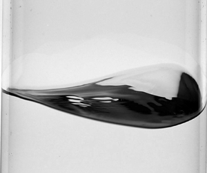
While operating a sweep in forcing frequency at a fixed forcing amplitude, we observe in the vicinity of the super-harmonic resonance three different kinds of motion, namely planar, irregular and swirling ones, whose occurrence depends on the forcing amplitude and frequency; see, for instance, the snapshots displayed on figure 8 or the videos provided among the supplementary movies available at https://doi.org/10.1017/jfm.2023.438.

Figure 8.

Images of the fluid free surface while the container is subjected to a longitudinal harmonic forcing of amplitude $a_x=\bar {a}_x/R \approx 0.23$ at various driving angular frequencies $\varOmega$ close to $\omega _{21}/2$. The fluid free surface is observed in the direction aligned with the container motion. For each driving frequency (a), (b) and (c), the time interval between two snapshots is about $T/4$, with $T=2 {\rm \pi}/ \varOmega$ the corresponding oscillation period. On each snapshot, the vertical middle axis is represented by a red dotted line. For a forcing frequency $\varOmega \approx 0.48 \omega _{21}$ (a) and $\varOmega \approx 0.52 \omega _{21}$ (c) the free-surface image at each time $t$ is mirror symmetric with respect to the middle vertical axis, the signature of a planar wave regime, while the symmetry is broken for $\varOmega \approx 0.50 \omega _{21}$ (c) revealing a swirling wave. Results are shown for (a) $\varOmega / \omega _{21}\approx 0.48$, (b) $\varOmega / \omega _{21}\approx 0.50$ and (c) $\varOmega / \omega _{21}\approx 0.52$.

For a given (and large enough) amplitude and starting from a frequency higher than a certain amplitude-dependent threshold $\varOmega _P(a_x)$, the free surface responds to the longitudinal harmonic forcing by displaying a planar dynamics such as shown in figure 8(c). When the critical frequency $\varOmega =\varOmega _P(a_x)$ is reached, the motion bifurcates to a swirling wave, which propagates along the container wall with a stationary amplitude; see figure 8(b). The wave can rotate either clockwise or anti-clockwise (both rotation directions were observed along the experiments). When the forcing frequency is further decreased below a critical frequency $\varOmega = \varOmega _H(a_x) \approx \omega _{21}/2 < \varOmega _P(a_x)$, the free surface exhibits an irregular dynamics, characterized by a switching between planar and swirling motion (not shown in figure 8). For forcing frequencies lower than a certain threshold $\varOmega < \varOmega _U(a_x)$, the free-surface motion stabilizes into a steady planar wave such as shown in figure 8(a). All together, these observations are qualitatively consistent with the outcomes of the WNL analysis in § 5, that predicts the existence of three different dynamical regimes – namely planar, irregular and swirling motions – for a longitudinal forcing frequency in the vicinity of $\omega _{21}/2$. One of the main purposes of the present experimental investigation is to determine the amplitude-dependent frequency bounds of these different regimes and to compare them to our theoretical prediction of the positions of the bifurcation points U (turning point), H (Hopf bifurcation) and P (Poincaré bifurcation) (see figures 5 and 6).

6.2.2. Procedure

Since the camera optical axis is aligned with the direction of the container motion, we note that a planar wave is characterized by its symmetry with respect to the vertical middle axis of the container image, whereas a swirling wave breaks this symmetry while travelling clockwise or anti-clockwise along the container walls; see figure 8.

We take benefit of these observations to build a more quantitative description of the free-surface dynamics, with the aim of identifying the various types of sloshing waves in the vicinity of the super-harmonic resonance. This can be done by exploiting the symmetry properties of the image of the free-surface response with respect to the vertical middle axis of the container image, and by characterizing the regularity of these waves as a function of the forcing parameters, so as to identify the irregular regime.

To do so, the time evolution of the free-surface dynamics is extracted from the movies along vertical directions that are mirror symmetric with respect to the vertical middle axis of the container image. Comparing the resulting temporal signals with each other allows one to discriminate between planar and swirling motions and to study the wave regularity.

The first step is to attach to each frame $t$ of a given movie, a Cartesian reference frame $(Y(t), Z(t))$, such that $Y(t)=0$ corresponds to the vertical middle axis of the container image, and that $Y(t)=R$ represents the right-hand side edge of the container image. To this end, the edges of the container are automatically detected in a dedicated Matlab program. The vertical $Z(t)$ axis ($Y(t)=0$) on the frame corresponding to time $t$ is then set as the middle line between these two edges, while the distance between both edges sets the scale of the horizontal direction $Y$. Note that we neglect the 4 mm thickness of the container wall.

A direction $y \in [-R, R]$ is then chosen to extract from each frame corresponding to time $t_i$, the intensity profile $I_{t_i}(y)$ along the vertical line $Y(t_i)=y$. The resulting intensity profiles are then plotted as a function of time to build an image $I(y)$ composed as $I(y)=[I_{t_1}(y), I_{t_2}(y),\ldots ]$, such as displayed in figure 9(c).

Figure 9.

General procedure for the analysis of the free-surface dynamics. (a) On each frame, the edges of the container are detected (black dotted lines) and the vertical $Z(t)$ axis is set as the middle line between these two edges, while the scale of the horizontal direction $Y(t)$ is fixed by the distance between both edges. (b) Schematic of the container illustrating the link between the Cartesian coordinate system $(Y(t), Z(t))$ attached to each frame and the cylindrical coordinates in the referential frame of the container. (c) Left: the intensity profile along a vertical line of coordinate $(Y(t)=y)$ with $y \in [-R, R]$ is then measured on each frame $t$ and plot as a function of time (here for $y=0$). The position of the front contact line at the azimuthal coordinate $\theta =\arcsin (y/R)=0$ as a function of time is highlighted in red. Right: frames from which the intensity profiles at times $t_i$ and $t_j$ on the left-hand side image, along the line $(Y(t)=0)$ (represented by a red dotted line), are extracted. At $t_i$, the wave is climbing the front wall of the container (with respect to the camera position) whereas at $t_j$ it reaches the back of the tank.

We note that at each time $t$, the intensity profile $I_{t}(y)$ contains the intersection of the front contact line image with the vertical axis $(Y(t)=y)$, that corresponds to the point of coordinates $(R, \theta, \eta (R, \theta, t))$ in the moving cylindrical frame of reference of the container, where $\theta =\arcsin (y/R)$ (see figure 9b). As a consequence, the final image $I(y)$ also contains the dynamics of the front contact line in the azimuthal direction $\theta$.

The resulting image $I(y)$ exhibits a periodic dark pattern that represents the free-surface response to the harmonic forcing, see an example in figure 9(c) in which $y=0$. Indeed, on each frame of the movie, the free surface appears as the darkest feature, so that the intensity profile along a given line $(Y(t)=y)$ actually represents the vertical extension of the free surface at time $t$ along this direction, which is maximal whenever the sloshing wave reaches its maximal elevation $\max _t \eta ( R, \theta, t)$ along the azimuthal direction $\theta = \arcsin (y/R)$ (in the front of the container with respect to the camera position, corresponding to $\theta \in ]-{\rm \pi} /2, {\rm \pi}/2[$) or along $\theta = {\rm \pi}- \arcsin (y/R)$ (in the back of the container). Furthermore, when the contact line reaches its maximal elevation in the front of the container, the free surface is imaged from below, so that it appears darker than when the maximal elevation is reached in the back, where the free surface is imaged from above; see the snapshots in figure 9(c). These observations allow us to identify in the image $I(y)$ the position as a function of time of the front contact line $\eta ( R, \theta, t)$, with $\theta =\arcsin (y/R)$, as highlighted in red in figure 9(c), and following the method detailed in Appendix D.

Note that this procedure does not give a quantitative access to the actual amplitude of the front contact line oscillations, since the intensity profiles $I_{t_i}(y)$ constituting the image $I(y)$ are simply juxtaposed with each other without rescaling the pixel width along the vertical direction. However, the position extracted from $I(y)$ of the image of the points of coordinates $\eta (R, \pm \theta, t)$ as a function of time still encloses the symmetry properties of the free-surface response, its regularity as well as its frequency content, which are the only quantities needed in order to identify the wave regimes.

6.3. Regularity and frequency content of the free-surface response

The resulting image $I(y)$ is then revealing of the free-surface dynamics $\eta (r, \theta, t)$ and, in particular, of its dynamics at the front wall $\eta (r=R, \theta =\arcsin (y/R), t)$. Figure 10(a–d) displays $I(0)$ for various forcing frequencies close to the super-harmonic resonance, at the same forcing amplitude. These images reveal that depending on the forcing frequency, the free-surface oscillations (dark periodic pattern) can be either regular (a), (c) and (d) – i.e. the oscillations are enclosed into an envelope of constant amplitude – or irregular (b) with a temporal modulation of the amplitude envelope. Therefore, the profiles $I(0)$ allow us to characterize the regularity of the sloshing wave and, in particular, to identify the irregular regime. The latter will be described in more detail in § 6.6, but such details are not needed for the identification of the irregular regime bounds, for which the analysis of the regularity property of the $I(0)$ pattern is sufficient. Therefore, in the following we will focus on the regular planar and swirling motions, which cannot be unambiguously distinguished from each other on the basis of the profiles $I(0)$.

Figure 10.

(a–d) Intensity profiles as a function of time along the vertical middle axis $(Y=0)$ – denoted $I(0)$ – for various forcing frequencies $\varOmega$ in the vicinity of the super-harmonic resonance $\varOmega \approx \omega _{21}/2$ at the same forcing amplitude $\bar {a}_x/R \approx 0.23$. In each case, the profile $I(0)$ is extracted from a movie whose recording has been started after about 50 oscillation cycles following each change in forcing frequency, thus ensuring that initial transients are filtered out (see also Appendix C). (e–h) Power spectral densities (PSD) – normalized by the maximal peak amplitude – corresponding to the front contact line dynamics as extracted from the profiles $I(0)$ displayed in panels (a)–(d).

Figure 10(e–h) displays the (normalized) power spectral densities of the front contact line dynamics $\eta (R, \theta =0, t)$ extracted from the profiles $I(0)$ (a–d). It appears that in all cases, the energy of the sloshing wave is massively distributed to its first (harmonic) and second (super-harmonic) component, while the contribution of higher modes is fairly negligible. This incidentally implies that the symmetry properties of a regular wave are directly linked to the symmetry properties of these two first oscillation modes.

In other words, a planar dynamics should necessarily consist in the superposition of two planar waves: a planar SC wave harmonically oscillating with the driving frequency $\varOmega$ and one super-harmonic planar DC wave oscillating at $\omega _{DC}= 2 \varOmega \approx \omega _{21}$. On the other hand, a swirling dynamics must contain at least one symmetry-breaking (swirling) component that, as predicted by the present WNL analysis, should correspond to the super-harmonic $\omega _{21}$ component.

6.4. Symmetry properties of the regular regimes: planar versus swirling waves

We now focus on the regular regimes, namely the steady planar and swirling motions. As stated before, the profiles $I(0)$ cannot discriminate between a planar and a swirling dynamics and instead only contain information on their regularity and their frequency content. To distinguish a planar from a swirling motion, we then compare the profiles along two ($Y \neq 0$) directions that are symmetric with respect to the vertical middle axis of the container image.

Figures 11(b), 11(d) and 11(f) show composite images, each produced using the Matlab function imshowpair applied to the pair $I(R/2)$ and $I(-R/2)$ for three different forcing frequencies that both result in a regular motion (the same forcing parameters as in figure 10a,c,d). Briefly, imshowpair $(I_\alpha,I_\beta )$ creates from a pair of greyscale images $I_\alpha$ and $I_\beta$, a red, green and blue (RGB) image where each pixel is represented by a RGB triplet, the R intensity being the intensity of the corresponding pixel in $I_\alpha$, and the G and B intensities being equal to the intensity of the corresponding pixel in $I_\beta$. A pixel where $I_\alpha$ and $I_\beta$ have the same intensity will be represented by a RGB triplet of the form $[a, a, a]$, where $a \in [0, 255]$, i.e. will appear as grey. On the contrary, if this pixel has a much larger intensity on $I_\alpha$ (respectively on $I_\beta$) than it has on $I_\beta$ (respectively on $I_\alpha$), it will appear in red (respectively in cyan) on the resulting composite image. The composite images displayed in figure 11(b,d,f) thus highlight in each case the differences between $I(R/2)$ and $I(-R/2)$. They are then a direct signature of the symmetry of the free-surface dynamics with respect to the vertical middle axis $(Y=0)$, and reveal two different kinds of motion: (i) a planar motion, for which $I(R/2)$ and $I(-R/2)$ perfectly overlap with each other due to the mirror symmetry of the wave; and (ii) a circular motion, characterized by a symmetry breaking between the right- and left-hand side free-surface dynamics: the maximum of the wave along $\theta =\arcsin (1/2)={\rm \pi} /6$ is indeed phase shifted with respect to the maximum of the wave along $\theta =-{\rm \pi} /6$, thus revealing a travelling wave propagating along the wall of the container.

Figure 11.

Symmetry properties of the stationary waves. (a,c,e) Images of the fluid free surface while the container is subjected to a longitudinal harmonic forcing of amplitude $\bar {a}_x/R \approx 0.23$ at various driving angular frequencies $\varOmega$ close to $\omega _{21}/2$: (a) $\varOmega \approx 0.48 \omega _{21}$, (c) $\varOmega \approx 0.50 \omega _{21}$ and (e) $\varOmega \approx 0.52 \omega _{21}$ (same forcing parameters as in figure 10a,c,d). For each driving frequency (a,c,e), the time interval between two snapshots is about $T/4$, with $T=2 {\rm \pi}/ \varOmega$ the corresponding oscillation period. On each snapshot, the vertical axes $(Y=R/2)$ and $(Y=-R/2)$ are represented by a blue and red dotted line, respectively. For a forcing frequency $\varOmega =0.48 \omega _{21}$ (a) and $\varOmega =0.52 \omega _{21}$ (e) the free-surface image at each time $t$ is mirror symmetric with respect to the middle vertical axis, while the symmetry is broken for $\varOmega = 0.50 \omega _{21}$. (b,d,f) Superposition of the intensity profiles as a function of time along the vertical axis $(Y=R/2)$ and $(Y=-R/2)$ – denoted $I(R/2)$ (in blue) and $I(-R/2)$ (in red), respectively – for the same forcing parameters as in figure 10(a, c, e). The grey regions show where $I(R/2)$ and $I(-R/2)$ have the same intensities.

To determine which $\omega$ component is responsible for the symmetry breaking induced by the swirling motion, we extract from $I(R/2)$ and $I(-R/2)$ the position of the front contact line as a function of time $\eta (R, \theta, t)$, where $\theta = \pm {\rm \pi}/6$; see figure 12(b,e). This makes it possible to compute the power spectrum of both signals, as well as the phase difference between the phase angle of their components that oscillate at the frequencies corresponding to their spectrum's first and second peaks (see figure 12c–f). A planar wave oscillating at a frequency $\omega$ is then characterized by the $\omega$ components of $\eta (R, {\rm \pi}/6, t)$ and of $\eta (R, -{\rm \pi} /6, t)$ being in phase with each other, while a swirling wave is characterized by a $m {\rm \pi}/3$-phase shift between the $\omega$ components of these signals, where $m$ denotes the azimuthal wavenumber of the swirling wave ($m=1$ for an harmonically oscillating SC wave, $m=2$ for a super-harmonic DC wave).

Figure 12.

Analysis of the steady-state free-surface dynamics under an harmonic forcing of amplitude $a_x=0.23$ and frequency (a–c) $\varOmega /\omega _{21} \approx 0.48$ and (d–f) $\varOmega / \omega _{21} \approx 0.50$. (a,d) Image of the free surface with vertical lines intersecting the image of the front contact line at the points of coordinates $(R, {\rm \pi}/6, \eta (R, {\rm \pi}/6, t))$ (blue arrows) and $(R, -{\rm \pi} /6, \eta (R, -{\rm \pi} /6, t))$ (red arrows) in the moving reference frame of the container. (b,e) Normalized elevation of the front contact line $\tilde {\eta }(R, {\rm \pi}/6, t)$ (blue dots) and $\tilde {\eta }(R, -{\rm \pi} /6, t)$ (red dots) extracted from the corresponding profiles $I(R/2)$ and $I(-R/2)$ (not shown here). The $\tilde {\eta }$ functions are defined according to $\tilde {\eta }(R, \theta, t)= (\eta (R, \theta, t)-\sigma ) / \delta$, where $\sigma =\min _t(\eta (R, \theta, t))+\max _t(\eta (R, \theta, t) )/2$ and $\delta =\max _t(\eta (R, \theta, t))-\min _t(\eta (R, \theta, t))$. (c,f) Left: power spectral densities of $\tilde {\eta }(R, {\rm \pi}/6, t)$ (blue dots) and of $\tilde {\eta }(R, -{\rm \pi} /6, t)$ (red dots). Right: absolute value of the phase shift between the components of $\tilde {\eta }(R, {\rm \pi}/6, t)$ and of $\tilde {\eta }(R, -{\rm \pi} /6, t)$ oscillating at the frequencies corresponding to the first peak ($\omega = \varOmega$) and to the second peak ($\omega = 2 \varOmega$) of the power spectra.

The Fourier analysis of the signals $\eta (R, {\rm \pi}/6, t)$ and $\eta (R, -{\rm \pi} /6, t)$ reveals that for forcing frequencies $\varOmega$ close to $\omega _{21}/2$, the free-surface motion mostly results from the combination of a SC wave harmonically oscillating at the forcing frequency $\omega _{SC}=\varOmega \approx \omega _{21}/2$, and of a super-harmonic DC wave oscillating at a frequency $\omega _{DC}=2 \varOmega \approx \omega _{21}$. From figures 12(c) and 12(f), it is clear that the SC wave is a planar wave for both planar (figure 12c) and swirling (figure 12f) dynamics, as revealed by the vanishing phase shift between the harmonic components of $\eta (R, {\rm \pi}/6, t)$ and $\eta (R, -{\rm \pi} /6, t)$ in both cases. On the other hand, the phase shift between the super-harmonic components is zero in the case of the planar dynamics, and close to $2 {\rm \pi}/3$ in the case of the swirling dynamics, the signature of a DC swirling wave. These observations are general to the whole range of forcing frequencies and amplitudes investigated along this study: in the vicinity of the super-harmonic resonance, the SC wave is always a planar wave, as revealed by the vanishing phase shift between the harmonic components of $\eta (R, {\rm \pi}/6, t)$ and $\eta (R, -{\rm \pi} /6, t)$ for both planar and swirling dynamics (this is also true in the case of the irregular regime, see later § 6.6). In the case of a regular dynamics, the DC wave is either a planar (for vanishing phase shift between the corresponding components) or a swirling wave (characterized by a $2 {\rm \pi}/3$ phase shift between the $\omega _{21}$ component of the right- and left-hand side signals), depending on the exact ratio between $\varOmega$ and $\omega _{21}$, as well as on the forcing amplitude $\bar {a}_x/R$.

6.5. Experimental estimate of regime bounds

From the above analysis, it appears that consistently with the predictions provided by our theoretical WNL analysis, the sloshing waves resulting from the longitudinal super-harmonic forcing of the container at a frequency $\varOmega \approx \omega _{21}$, consist in the superposition of a planar SC wave, harmonically oscillating with the forcing at $\omega =\varOmega$, and of a DC wave, which can exhibit either a planar, irregular or swirling dynamics.

Having identified the three different regimes for the free-surface dynamics in the vicinity of the super-harmonic resonance, we can now experimentally determine their stability regions in the $(\varOmega /\omega _{21}, a_x)$ space. To do so, we fix the forcing amplitude while operating a frequency sweep from high to low frequencies, within the range $\varOmega /\omega _{21} \in [0.45, 0.53]$, by frequency decrements of 10 mHz. Note that a downward frequency sweep ensures recovery of the stability bound between the super-harmonic planar and swirling regimes, as the transition in this direction occurs exactly at the threshold frequency $\varOmega _P(a_x)$ below which the super-harmonic planar motion becomes unstable. On the contrary, since the super-harmonic swirling wave is still stable for frequencies larger than $\varOmega _P(a_x)$ (hysteresis), an upward frequency sweep will maintain the system's response on the swirling branch, thus, it is not suitable to experimentally detect the bifurcation point P. The downward frequency sweep also enables one to detect the bounds that separate the irregular regime from steady planar ($\varOmega = \varOmega _U(a_x)$) and swirling motions ($\varOmega = \varOmega _H(a_x)$).

This procedure is applied for various forcing amplitudes $a_x \in [0.05, 0.4]$, enabling us to build the stability regions diagram displayed on figure 13. All together, the experimental measurements are in very good quantitative agreement with the theoretical regime bounds for $a_x > 0.15$, below which the super-harmonic irregular and swirling regimes appear to be suppressed by dissipative mechanisms, e.g. viscous dissipation occurring in the fluid bulk, sidewall and free-surface boundary layers (Case & Parkinson Reference Case and Parkinson1957; Miles Reference Miles1967; Raynovskyy & Timokha Reference Raynovskyy and Timokha2020; Bongarzone et al. Reference Bongarzone, Viola, Camarri and Gallaire2022b) as well as in the neighbourhood of the moving contact line (Keulegan Reference Keulegan1959; Dussan Reference Dussan1979; Hocking Reference Hocking1987; Cocciaro, Faetti & Festa Reference Cocciaro, Faetti and Festa1993; Viola & Gallaire Reference Viola and Gallaire2018). This last contribution is likely to be important since no particular precautions, such as wall treatment or pre-wetting, have been taken in order to minimize contact angle hysteresis. Below this threshold amplitude, experiments have shown a vanishing super-harmonic contribution to the dynamics, with a harmonic planar motion produced by the SC wave only and well described by the potential linear model, thus suggesting that the DC wave has been entirely killed by the dissipative mechanism. Note that such a suppression of the DC dynamics at low forcing amplitude is reminiscent of what was observed by Reclari et al. (Reference Reclari, Dreyer, Tissot, Obreschkow, Wurm and Farhat2014) for circular shaking.

Figure 13.

Estimates of regime bounds in the $(\varOmega /\omega _{21},a_x)$ plane for a container of diameter $D=0.172\ \text {m}$, filled to a depth $H=1.3$, driven longitudinally and super harmonically at a frequency $\varOmega \approx \omega _{21}/2$: comparison between the theoretical predictions (solid lines) and experimental measurements (markers). Grey thick solid lines: present theoretical predictions. Black empty squares: super-harmonic planar motion. Black crosses: irregular regime. Black filled circles: super-harmonic swirling motion.

6.6. Irregular regime

In this section we provide a more thorough description of the irregular regime. When fixing the forcing frequency slightly below $\omega _{21}/2$ and progressively increasing the forcing amplitude, the free-surface response is first very regular and displays a planar dynamics for low enough forcing amplitudes. Above a threshold amplitude, the dynamics becomes irregular and at large enough amplitudes, the response is again regular, but consists in a swirling motion. Figure 14(a) displays the free-surface response along the vertical middle axis $Y=0$ for increasing forcing amplitudes at a fixed forcing frequency $\varOmega \approx 0.496 \omega _{21}$. The regular regimes (top and bottom panels) are characterized by a constant amplitude of the free-surface oscillations. In contrast, the oscillations of the free surface for intermediate forcing amplitudes (second and third panels) are enclosed into a quasi-periodic envelope, whose frequency linearly increases with the forcing amplitude (see figure 14(b) and Appendix D for the methodology used to compute the envelope). This is very reminiscent of the observations by Royon-Lebeaud et al. (Reference Royon-Lebeaud, Hopfinger and Cartellier2007) of the irregular regime present in the vicinity of the harmonic resonance under longitudinal forcing. Note that these features are also quantitatively recovered by proceeding with a downwards amplitude sweep. In particular, upward and downward forcing amplitude sweeps provide the same threshold amplitudes between planar and irregular dynamics, and between irregular and swirling regimes. Furthermore, the frequency of the main peak in the power spectrum of the amplitude envelope seems to be a robust feature that does not depend on the sweep direction; see figure 14(b).

Figure 14.

(a) Intensity profiles $I(0)$ for various forcing amplitudes and the same forcing frequency $\varOmega \approx 0.496 \omega _{21}$. The oscillations of the free surface are enclosed into an envelope, plotted in black on top of the images. (b) Left: frequency of the main peak in the power spectrum of the envelope (adimensionalized by the forcing frequency $\bar {\varOmega }/2{\rm \pi}$) as a function of the forcing amplitude $a_x$, for the same angular forcing frequency $\varOmega \approx 0.496 \omega _{21}$, and for upwards (white markers) and downwards (black markers) amplitude sweeps. When the envelope is a straight line (as it is the case here for $a_x < 0.15$, which corresponds to a regular planar dynamics of the free surface), the power spectrum is flat and we set the corresponding frequency equal to zero. For $a_x \approx 0.40$, the power spectrum of the envelope is dominated by a low amplitude and small frequency noise, causing a brutal decrease of the ‘burst’ frequency, thus indicating a transition from irregular to regular swirling motion. Right: power spectra of the envelope for $a_x\approx 0.12$, $a_x \approx 0.23$ and $a_x \approx 0.40$. (c) Correlation between $I(R/2)$ and $I(-R/2)$ as a function of time for the same set of forcing parameters as in (a). (d) Left: superposition of $I(R/2)$ (blue) and $I(-R/2)$ (red); right: position of the front contact line $\eta ( R, \pm {\rm \pi}/6, t)$ as a function of time extracted from $I(-R/2)$ (red curve) and from $I(R/2)$ (blue curve). The signals presented in (d) are taken from the full signals used to compute their correlation in (c) for $a_x \approx 0.23$, over the time ranges highlighted in blue and denoted as (1) (maximum of correlation) and (2) (minimum of correlation). (e,f) Normalized power spectra of $\eta (R, -{\rm \pi} /6, t)$ (red curve) and of $\eta (R, {\rm \pi}/6, t)$ (blue curve), and the absolute value of the phase shift between their harmonic and super-harmonic components, where the dynamics of $\eta (R, \pm {\rm \pi}/6, t)$ is considered over (e) time range (1) and (f) time range (2).

To gain more insight on this irregular dynamics, we compute at each time $t_i$ the spatial correlation between $I_{t_i}(R/2)$ and $I_{t_i}(-R/2)$, which we refer to as ${\rm corr} (t_i)$,

(6.1)\begin{equation} {\rm corr}(t_i)=\frac{\displaystyle \sum_n (I_{t_i, n}(R/2)-\bar{I}_{t_i}(R/2))(I_{t_i, n}({-}R/2)-\bar{I}_{t_i}({-}R/2))}{\displaystyle \sqrt{\sum_n (I_{t_i, n}(R/2)-\bar{I}_{t_i}(R/2))^2\sum_n (I_{t_i, n}({-}R/2)-\bar{I}_{t_i}({-}R/2))^2}}, \end{equation}

where $n \in [1, N]$, with $N$ the number of pixels in the vertical direction, and $\bar {I}_{t_i}(y)$ represents the mean of the $N$-element vector $I_{t_i}(y)$. A high and constant correlation is a signature of a steady planar motion, while a low but still constant correlation is characteristic of the steady swirling regime. At intermediary forcing amplitudes – i.e. in the irregular regime – the correlation is a quasi-periodic function of time, with the same quasi-period as the envelope; see figure 14(c).

A comparison between $I(R/2)$ and $I(-R/2)$ on time ranges corresponding to the maximum and minimum of the correlation function reveals that in the time interval where the signals are highly correlated, the motion is planar like (although irregular), while in the time range where they are poorly correlated, the maxima of the right- and left-hand side signals are phase shifted with respect to each other, thus reflecting the presence of a swirling wave; see figure 14(d).

This is further confirmed by the power spectra of the front contact line dynamics along the azimuthal directions $\theta =\pm {\rm \pi}/6$, extracted from $I(R/2)$ and $I(-R/2)$, on time ranges where these signals are highly correlated and where they are poorly correlated; see figure 14(e,f). In both cases, the sloshing wave contains a planar SC wave, as revealed by the vanishing phase shift between the harmonic components of $\eta (R, {\rm \pi}/6, t)$ and $\eta (R, -{\rm \pi} /6, t)$. The wave also contains a super-harmonic component that is responsible for the switching between a planar-like motion (vanishing phase shift between the $\omega _{21}$ components of the $\eta (R, {\rm \pi}/6, t)$ and $\eta (R, -{\rm \pi} /6, t)$ signals, figure 14e) and a swirling dynamics (rotating, symmetry-breaking wave that is super-harmonically oscillating at $\omega \approx \omega _{21}$, figure 14f).

This is again very similar to the features of the irregular regime in the vicinity of the harmonic resonance described by Royon-Lebeaud et al. (Reference Royon-Lebeaud, Hopfinger and Cartellier2007) that relate the ‘bursts’ in the free-surface oscillation amplitude to the quasi-periodic occurrence of a swirling wave. However, in the case of super-harmonic resonance the irregular regime consists here in the superposition of a stable planar SC wave and of a super-harmonic DC dynamics. The latter is responsible for the irregularity of the total dynamics, by quasi-periodically switching between super-harmonic planar and swirling motions.

6.7. Wave amplitude saturation: theoretical predictions vs experiments

In this last section we provide a more quantitative comparison in terms of wave amplitude saturation between the theoretical predictions according to (5.13) and the experimental measurements. On this point, the dimensional wave amplitude, ${\rm \Delta} \bar {\delta }=\max _{\theta,t}\eta (r=R,\theta,t)- \min _{\theta,t}\eta (r=R,\theta,t)$, is experimentally measured by fixing the forcing amplitude while operating a frequency sweep in two directions. A backward sweep is used so as to follow the right lower planar branch until the sub-critical jump-up transition to swirling ($P$: Poincaré bifurcation) occurs ($\varOmega =\varOmega _{P}(a_x)$). On the other hand, an upward sweep is performed in order to maintain a stable super-harmonic swirling response from bifurcation point $H$ ($\varOmega =\varOmega _{H}(a_x)$) and beyond the threshold frequency $\varOmega =\varOmega _{P}(a_x)$, above which the super-harmonic planar and swirling motions are both stable solutions (right region in the stability chart of figure 13).

For each set of forcing parameters $(a_x, \varOmega /\omega _{21})$, the height in pixel of the wave crest (respectively trough) on the front wall is manually extracted from the corresponding movies and is compared, in the same frame it is extracted from, to the height of the fluid at rest (flagged by a black mark on the container, also used as a scale) to obtain the maximal (respectively minimal) front contact line elevation $\max _{\theta,t}\eta (r=R,\theta,t)$ (respectively $\min _{\theta,t}\eta (r=R,\theta,t)$). This value is converted into metres using the conversion factor provided by the black scale. The resulting amplitude ${\rm \Delta} \bar {\delta }$ is then averaged over three to five cycles of oscillations and finally normalized by the container radius $R$.

The experimental dimensionless wave amplitude ${\rm \Delta} \delta = {\rm \Delta} \bar {\delta }/R$ as a function of the forcing frequency for various forcing amplitudes is displayed in figure 15 together with the theoretical WNL prediction (5.13) (light blue solid lines) and with the linear potential solution (3.4) for comparison (black dashed line).

Figure 15.

Quantitative comparison with experimental measurements in terms of finite amplitude saturation for various non-dimensional forcing amplitudes, $a_x$. Black dotted lines: linear potential solution according to (3.4) and (3.5). Light blue solid lines: stable planar and swirling branches predicted by the present WNL model according to (5.13). Markers: experimental measurements. Black empty squares correspond to planar motion whereas black filled circles refer to swirling dynamics. Results are shown for (a) $a_x=0.1628$, (b) $a_x=0.1861$, (c) $a_x=0.2093$, (d) $a_x=0.2325$, (e) $a_x=0.2558$ and (f) $a_x=0.2791$.

The experimental data associated with the two planar branches compare generally well with the present WNL prediction, although the WNL theory slightly underestimates the wave amplitude in the swirling regime. Such an underestimation is not necessarily produced by overlooked nonlinear mechanisms, but it could be instead ascribed to the linear superposition of viscous modes, whose phase shift's characterization would require a dedicated theoretical viscous analysis. The same holds for the asymmetry experimentally observed in the DC wave profile reported in figures 9(c), 11(d) and 12(e).

We recall from § 5 that, at leading order, the wave solution in these two branches is made by the superposition of two planar waves, i.e. an harmonic planar SC component, oscillating in space and time as $\cos {(\varOmega t)}\cos {\theta }$, and a super-harmonic planar DC component, characterized by $\cos {(2\varOmega t+\varPhi )}\cos {2\theta }$, with a phase $\varPhi ={\rm \pi}$ in the left branch and $\varPhi =0$ in the right one. The information on the phase $\varPhi$ is not directly discernible from the amplitude plot of figure 15, but it is contained in the snapshots sequence reported in figure 11(a) for $\varOmega /\omega _{21}<0.5$ and (e) for $\varOmega /\omega _{21}>0.5$. Due to the temporal periodicity of the SC wave, snapshots taken at $t=T/4={\rm \pi} /2\varOmega$ and $t=3T/4=3{\rm \pi} /2\varOmega$ represent temporal nodes for the harmonic component, so that, as a first-order approximation, only the DC component, whose azimuthal spatial structure reads $\cos {({\rm \pi} +\varPhi )}\cos {2\theta }$, is instantaneously left. It is then clear that for $\varOmega /\omega _{21}<0.5$ and $\varPhi ={\rm \pi}$, the free surface maximum is reached at the azimuthal coordinates $\theta =0$ and ${\rm \pi}$, whereas the minimum is at $\theta =\pm {\rm \pi}/2$ (vice versa for $\varOmega /\omega _{21}>0.5$ and $\varPhi =0$). This produces the concave and convex shapes in the instantaneous free surface displayed in figures 11(a) and 11(e), respectively.

Consistently with the stability chart in figure 13 obtained through a backward frequency sweep, the threshold frequency $\varOmega _H(a_x)$, at which the swirling branch becomes stable from lower driving frequency $\varOmega$, is correctly detected. Furthermore, the upward sweep allows us to detect also the jump-down transition from the swirling to the lower right planar branch.

The occurrence of the jump-down transition was to be expected as it is produced by dissipative mechanisms (see also § 6.5), which are overlooked by the present inviscid analysis. The associated damping, which is a function of the wave amplitude and of the forcing acceleration amplitude (see Raynovskyy & Timokha (Reference Raynovskyy and Timokha2018b), Raynovskyy & Timokha (Reference Raynovskyy and Timokha2020) and the discussion in Appendix A of Bongarzone et al. Reference Bongarzone, Guido and Gallaire2022a), is responsible for the modulation in the phase lag between the external driving and the wave response, which was shown by Bäuerlein & Avila (Reference Bäuerlein and Avila2021) (for unidirectional sloshing waves in a rectangular container) to be of crucial importance for a correct prediction of the jump-down frequency.

The damping coefficient could be tentatively fitted from experiments and phenomenologically introduced a posteriori in amplitude (5.9a) and (5.9b) as done in Appendix A of Bongarzone et al. (Reference Bongarzone, Guido and Gallaire2022a). Nevertheless, the jump-down transition in the cases examined in this section (see figure 15) was seen to be extremely sensitive to the frequency sweeping rate. A decrease in the frequency step increment from 5 mHz to 1 mHz (used to produced the swirling branch in figure 15) was observed to give different jump-down frequencies. This is also expected as it is known from the literature that in the multi-solution range, the characteristic of the response mainly depends on the sweep rate (Park, Do & Lopez Reference Park, Do and Lopez2011; Bourquard & Noiray Reference Bourquard and Noiray2019; Yu et al. Reference Yu, Tang, Xiong and Yang2020). Since we did not try frequency increments smaller than 1 mHz, the jump-down frequency predictions as shown in figure 15 are not entirely reliable for fitting the damping at stake in the experiments.

In spite of such limitations, the WNL model is seen to describe fairly well the experimental swirling branch until the measured jump-down frequency. A relatively small departure of the swirling response from the theoretical prediction is typically observed at larger driving amplitude for increasing wave frequency. In agreement with previous studies (Dodge et al. Reference Dodge, Kana and Abramson1965; Ibrahim Reference Ibrahim2005; Bäuerlein & Avila Reference Bäuerlein and Avila2021), our experiments reveal that this is due to the progressive steepening and broadening of the wave crest and troughs, respectively, in the vicinity of the container wall. This nonlinear mechanism eventually becomes strong enough for the WNL model to lose accurateness.