1. INTRODUCTION
Aviation has grown from the first commercial flight in 1914 to the present with more than 120,000 landings and 12 million passengers per day globally in 2018, according to the Air Transport Action Group (ATAG, 2018). Forecasts on the increase of commercial flights are optimistic, with the number of passengers expected to double by 2030. Despite the large number of flight operations, the amount of accidents and incidents remains low. However, their consequences can be very dramatic in both losses of lives and economic costs. According to Boeing (2017), there were a total of 1948 accidents in the period 1959–2016 worldwide (388 from 2007 to 2016). 31·98% of those accidents had fatal consequences (15·98% in 2007–2016).
In the last 50 years, there has been a major reduction in the number of accidents. This is due to improvements in technology and risk management. The research and development departments of aviation companies and the international aviation agencies have made an effort to evaluate various risks. Since these cannot be fully eliminated, the main objective is to provide procedures for their efficient and optimal management. It was not until 2006 that the International Civil Aviation Organization (ICAO) published the first risk management guidelines (ICAO, 2006). The proposals were widely accepted by air transport authorities and aviation manufacturers. Two updates were released in 2009 and 2013. However, the number of accidents (especially runway overruns) worsened in the period 1992–2011 with the increase in flight operations (Rosenkrans, Reference Rosenkrans2012).
There are many types of accidents and incidents in aviation see, for example, Evans (Reference Evans2014). Some of the most serious happen during landing. This phase is critical as pilots must consider many factors and make the right decisions quickly (Gerard, Reference Gerard2006; You et al., Reference You, Ji and Han2013; Wang et al., Reference Wang, Wu and Sun2014; Boyd and Stolzer, Reference Boyd and Stolzer2016). According to Boeing (2016), in the last ten years 49% of accidents in commercial flights occurred during the final approach or landing. There are many factors affecting landing manoeuvres. Jenkins and Aaron (Reference Jenkins and Aaron2012) point to the following causes as the most relevant in landing accidents: unstabilised approach, tail or crosswind, high speed, long landing or poor use of reverse thrust. Other authors such as Chang et al. (Reference Chang, Yang and Hsiao2016), Hunter et al. (Reference Hunter, Martinussen, Wiggins and O'Hare2011) and Ahmed et al. (Reference Ahmed, Abdel-Aty, Lee and Yu2014) focus on environment, containment runways and weather as risk factors. Rosenkrans (Reference Rosenkrans2012) defined some recommendations that should be followed to reduce risks, such as crossing the threshold at the right height at moderate speed, beginning the landing at the specified zone and properly using reverse thrust and other braking systems. The Flight Safety Foundation (FSF) also provides recommendations to reduce the risk of runway excursions (FSF, 2009).
Runway excursions happen during landings when an aircraft lands short (undershoot) exceeds the end (overrun) or the side (veer-off) of the runway (see Wong et al., Reference Wong, Pitfield, Caves and Appleyard2006). In the period 2010–2014, 87 out of 415 accidents with damage were runway excursions, resulting in a total of 174 deaths according to the International Air Transport Association (IATA) (IATA, 2015). Overruns are especially relevant since they account for 22% of all accidents and incidents in air transportation, and 44% of runway excursions are overruns.
There are many risk factors potentially affecting runway overrun. To discover them, it is necessary to analyse the conditions before landing and the information obtained after an accident occurs. Van Es (Reference Van Es2005) analysed data from 400 runway overruns covering 35 years. Later, Van Es et al. (Reference Van Es, Tritschler and Tauss2009) dealt with identifying the main factors in runway overruns and proposed a risk index. Ayres et al. (Reference Ayres, Shirazi, Carvalho, Hall, Speir, Arambula, David, Gadzinski, Caves, Wong and Pitfield2013) described a frequency model to determine the location of runway overruns and analysed the influence of several risk factors.
To prevent these risks, it was recommended by ICAO (2018) to build Runway Safety Areas (RSAs), which help to reduce damage in overruns and also in overshoots. In this context, Arnaldo Valdés et al. (Reference Arnaldo Valdes, Gomez Comendador, Mijares Gordun and Saez Nieto2011) proposed a probability-based approach to estimate risks in both overrun and undershoot, offering solutions for the construction of RSAs. Drees et al. (Reference Drees, Wang and Holzapfel2014) analysed the influence of some aerodynamic variables and proposed a sensitivity analysis method based on simulated data. Benedetto et al. (Reference Benedetto, D'amico and Tosti2014) analysed runway deflection and rutting, trying to reduce the overrun risks with cleared and graded areas. Also, Wilke et al. (Reference Wilke, Majumdar and Ochieng2014) provided a risk analysis based on the runway surface. An overrun prevention system based on the alert box defined by Ryan and Brodegard (Reference Ryan and Brodegard2003) has been patented.
Frequency models have been widely used for risk assessment in aviation accident analysis. However, they provide a descriptive perspective and do not allow one to relate multiple variables from a probabilistic point of view. Bayesian Belief Networks or simply Bayesian Networks (BNs) (Cowell et al., Reference Cowell, Dawid, Lauritzen and Spiegelhalter2006) constitute an especially interesting probabilistic method for constructing risk scenarios related to aviation accidents.
Bayesian modelling is not very common in aviation literature, but it is very promising. For instance, Feng et al. (Reference Feng, Sahin and Karson2009) applied it for aviation baggage screening, Ronald and Fabian (Reference Ronald and Fabian2014) for aviation delay modelling and Andres et al. (Reference Andres, Luxhoj and Coit2005) for aviation human-system risk and safety. In particular, BN's have been applied in several settings for the purpose of supporting probabilistic predictions in aviation risk analysis. For example, Luxhøj and Kauffeld (Reference Luxhøj and Kauffeld2003) presented a new risk model for aviation systems that evaluates the impact of including new technologies to reduce the negative consequences of accidents. This BN model was implemented in the Probabilistic Decision Support System (PDSS) software package to evaluate risks of new technology interventions. Brooker (Reference Brooker2011) considered expert opinions to estimate rare events in a BN framework and Gu (Reference Gu2009) used BNs to analyse the relationships among the main risk factors (helicopter technical dependability measures and environmental features) for helicopter accidents.
The focus of this paper is on risk analysis for prevention of overrun excursions based on a real dataset. Obtaining real data from aviation companies is very difficult (see, for example, Kirkland et al. (Reference Kirkland, Caves, Humphreys and Pitfield2004)) although its availability would clearly be very useful in that it would provide accurate information. We perform a BN model selection to fit the available data. The optimal BN is then used to define several risk scenarios that allow us to assess the influence of some states of the variables involved. This also lets us rank the corresponding runways based on the risk of overrun excursion. This is based on the probability of the event that the remaining distance to the end of the runway is less than 2,500 feet when the velocity is greater or equal to 80 knots. The higher this probability, the higher the risk of runway overrun.
2. METHODS
2.1. Data available
A data collection process was performed based on landing operations on three runways. They have similar operational conditions with landing lengths of less than 7,200 feet. Their locations cannot be divulged for confidentiality reasons. The runways will be denoted RwA, RwB, and RwC.
A total of 266 landing operations over a period of 10 months were recorded for the same airline and aircraft type. The main variable of interest was the remaining length (in feet) of the runway when the aircraft has a speed of 80 knots, see, for example, Burin (Reference Burin2011). This variable, denoted Rw80, allows us to identify the risk of not finishing within the runway boundaries. According to the FSF guidelines (Burin, Reference Burin2011), the risk of an accident increases considerably when the aircraft has a speed greater than 80 knots when it has a remaining landing distance of 2,000 feet. The other variables recorded are:
• Height: This variable represents the height at threshold in feet over the runway.
• DiffIV: This represents the difference between the indicated airspeed and the final approach speed at threshold, measured in knots. The indicated airspeed is read directly from the instruments, whereas the final approach speed represents the airspeed to be maintained down to 50 feet over the runway threshold (plus corrections for wind).
• Tailwind: This is the tailwind at threshold, measured in knots.
• Xwind: This represents the crosswind at threshold, measured in knots. Xwind and Tailwind are of interest specifically for landing overruns. Other problems such as veer off or undershoot would also be affected by headwind but they are not included in this research.
• Trevf: This variable describes the time in seconds that the maximum reverse thrust is operated to provide deceleration.
• Rw. This identifies the landing runway: A, B or C.
• Approach: This indicates whether the approach is stabilised or not.
• Abrake: This represents the autobrake activation, with three possible values: not activated, low, or medium.
It is also important to define how a stabilised approach was defined. According to the FSF, IATA and Eurocontrol, an approach is stabilised when all the following criteria are met (see https://www.skybrary.aero/index.php/Stabilised_Approach):
• The aircraft is on the correct flight path.
• Only small changes in heading/pitch are necessary to maintain the correct flight path.
• The airspeed is not more than Velocity of Reference (VREF) + 20kts indicated speed and not less than VREF.
• The aircraft is in the correct landing configuration.
• Sink rate is no greater than 1,000 feet/minute; if an approach requires a sink rate greater than 1,000 feet/minute a special briefing should be conducted.
• Power setting is appropriate for the aircraft configuration and is not below the minimum power for the approach as defined by the operating manual.
• All briefings and checklists have been conducted.
In Section 4, this dataset will be analysed. We next describe the methods used for data analysis.
2.2. Statistical methods
We performed a statistical data analysis of the database. Firstly, exploratory techniques were used. In order to analyse the relationships between pairs of variables, different hypothesis tests were considered. A chi-squared test was applied to determine the possible association between the use of autobraking and the runway. A Fisher exact test was applied for the same purpose between approach stabilisation and the runway (as, in this case, the applicability conditions for a chi-squared test were not met). For two quantitative variables, Spearman correlation coefficients and testing were considered to analyse the strength of the association between variables (as the conditions for a Pearson test were not met). Finally, since Analysis of Variance (ANOVA) applicability conditions could not be assumed, a nonparametric alternative was applied. Specifically, the Kruskal-Wallis test (Kruskal and Wallis, Reference Kruskal and Wallis1952) was used to analyse the differences between each quantitative variable for the different runways. Pairwise comparisons were performed using a Mann-Whitney U test (Mann and Whitney, Reference Mann and Whitney1947) with a Bonferroni correction (Dunn, Reference Dunn1961).
A BN is a directed acyclic graph that defines a joint probability distribution for a set of features. Each node represents a variable and the arcs represent causal dependence between nodes. For each node, the distribution of its variable conditioned on its predecessors in the net is defined; it is called Conditional Probability Distribution (CPD). The complete network defines a joint probability distribution, based on the CPD and the graph relationships. This joint distribution is given by the product of the probabilities of each node conditioned on the value of its predecessors. BNs are specifically defined for modelling uncertain and complex risk domains. As they are defined strictly in terms of probabilities and conditional independence statements, their main use would be to analyse different conditional probability scenarios (Akhtar and Utne, Reference Akhtar and Utne2014). They can also be applied to prediction problems (see Banghart et al., Reference Banghart, Bian, Strawderman and Babski-Reeves2017). One of the main advantages of its use is that it provides both a causal and probabilistic model, thus it is perfect for providing information supported by experts' knowledge combined with conditional probabilities, resulting in a human-interpretable decision tool (Heckerman, Reference Heckerman2008).
BNs take all the variables in the database into consideration conjointly to construct risk scenarios. For this task, quantitative variables were discretised by separating them into non-overlapping intervals. For comparative purposes, six algorithms for BN were considered in a model selection framework: Bayesian Search, Essential Graph Search, Tree Augmented Naive Bayes, Augmented Naive Bayes, Simple Naive Bayes, and Greedy Thick Thinning, all of which were implemented in Genie (Byoung-Hee, Reference Byoung-Hee2014), which was also used for BN calculations. The performances of the algorithms when applied to the current database were compared through five-fold cross-validation using 1,000 repetitions (Kim, Reference Kim2009). The accuracy and the Area Under the Receiver Operating Characteristic (ROC) Curve (denoted AUC) were considered as goodness-of-fit measures. The ROC curve presents sensitivity in the y-coordinate versus one-specificity or false positive rate in the x-coordinate. The AUC is a measure of model performance used for classification models that varies in the range [0, 1]. When it is close to 1, it means that the algorithm is able to adequately identify the risky cases in which the remaining length of the runway is reduced and becoming a risk for the landing. As we are studying the remaining runway over and above 2,500 feet, this measure is especially interesting. It is one of the most used performance metrics when combined with accuracy rate.
The algorithm best fitting these data was Greedy Thick Thinning (Dash and Cooper, Reference Dash and Cooper2004). This is a graph-structure learning algorithm that searches for a Directed Acyclic Graph (DAG) which maximises the scoring function in the search space of all DAGs containing the finite set of variables. In BN structure learning, a scoring function measures how good a given network matches the data set. In this case, the score was calculated with the Bayesian Dirichlet equivalent uniform (BDeu) criterion. This is based on a Dirichlet distribution with a weakly informative uniform prior, see Cooper and Herskovits (Reference Cooper and Herskovits1992) and Silander et al. (Reference Silander, Roos, Kontkanen and Myllymaki2008). The Greedy Thick Thinning algorithm starts with an empty graph at a specific point in the structure space. In order to maximise the Bayesian score, it continues adding neighbouring arcs until no additional arc improves the score. It then starts to remove arcs until a local optimum is achieved. The first process is known as thickening; the second one as thinning. The result is the model that best fits the given data.
The BN produced by this algorithm will be used in the following section to construct risk scenarios through evidence propagation, one of the most powerful features of Bayesian networks. With this technique, probabilities at each node can be updated via two-way propagation of new information throughout the structure. The resulting probabilities will be expressed as percentages. In each scenario, a set of evidences (represented by 100% probability in some categories) is defined according to very risky or very safe situations. We study how these evidences influence the probabilities of runway excursions. Probability estimates for different scenarios are reported in two tables.
3. RESULTS AND DISCUSSION
We shall present first the main exploratory results, and then we shall apply the Bayesian-network-based approach to perform a risk analysis.
3.1. Exploratory analysis
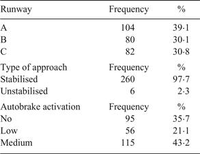
Table 1 lists the frequency distributions of the variables describing runway, type of approach, and autobrake activation. Runway A is the most frequently used, receiving almost 40% of landing operations. Autobraking was not activated in more than one third of the operations, while unstabilised approaches were rare (2·3%).
Frequency distributions for qualitative variables

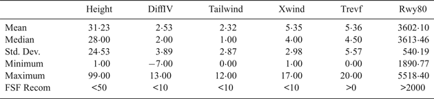
Descriptive statistics of the relevant quantitative variables are presented in Table 2. The global recommendations FSF (2009) for reducing the risk of runway excursions are largely satisfied. For instance, both crosswind and tailwind tend to be under 10 knots; the speed difference tends to be less than 10 knots; the height, less than 50 feet, and there remains a length of runway greater than 2,000 feet when a speed of 80 knots has been reached. However, some landings did not satisfy the recommendations. Specifically, 6% and 0·8% of the landing operations were performed with crosswind and tailwind speeds greater than 10 knots, respectively; 2·3% were unstabilised; 1·9% had speed differences greater than 10 knots and, finally, 19·9% had heights at threshold above 50 feet.
Descriptive statistics of quantitative variables involved

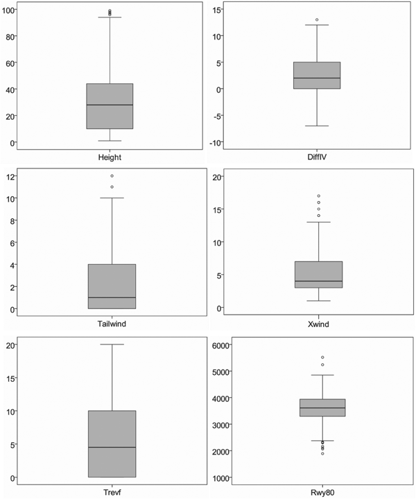
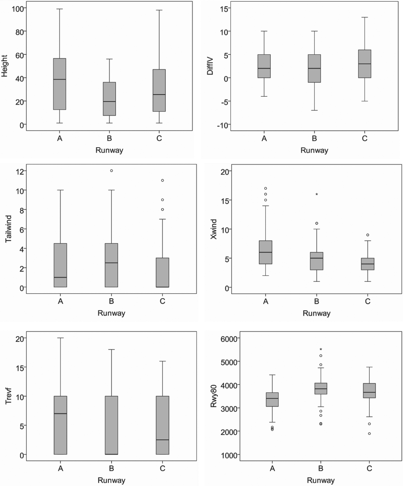
Figure 1 shows box plots of the quantitative variables. The frequency distributions for maximum reverse thrust, tailwind, crosswind, and height have a right-tailed asymmetry. All variables except maximum reverse thrust present outliers. For Rwy80, the most worrisome outliers are located close to 2,000 feet. The height shows quite a few risky operations above 50 feet, some of them close to 99 feet. Finally, there are more crosswind than tailwind outliers above the maximum recommendation of 10 knots.
Box plots for: height, DiffIV, Tailwind, Xwind, Trevf, and Rwy80.

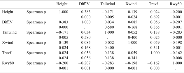
Table 3 presents Spearman correlation coefficients for pairwise variables and their p-values (p). Six, out of fifteen, pairwise variable associations, were not significant; the greatest significant correlation coefficient was 0·383 (p < 0·001), obtained for speed difference and height. The variable Rwy80 has significant negative correlations with all the other variables, showing that the remaining length of the runway at 80 knots decreases as height, crosswind, tailwind, speed difference or maximum reverse thrust increases. An increase in any of these variables would suggest an increase in the risk of runway excursions. Nevertheless, none of these associations seems strong.
Pairwise Spearman correlation coefficients and two-sided p-values

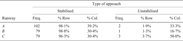
Aviation safety experts stress that landing operations are influenced by the characteristics and state of the runway (Daidzic and Shrestha, Reference Daidzic and Shrestha2008). Table 4 provides a comparison between stabilised and unstabilised landings depending on the runway used. The highest number of unstabilised landings among the three runways observed occurred in Runway C. However, Fisher's exact test showed that there is no significant association between the type of approach and runway (p = 0·674).
Type of approach by runway

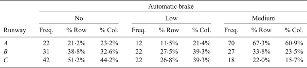
On the other hand, Table 5 presents the contingency table for autobrake activation and runway. Autobraking was used with less intensity on Runway C and with greater intensity on Runway A. In this case, the chi-squared test showed a significant statistical association between use of autobraking and runway (p < 0·001).
Autobrake activation by runway

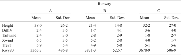
Table 6 provides descriptive statistics of the quantitative variables by runway. Some differences can be observed. Landing operations performed on Runway A had the greatest height, crosswind, and maximum reverse thrust averages. This runway also had the shortest remaining length average when the speed had fallen to 80 knots (although the minimum observation happens in Runway C), further evidence that this runway had the greatest excursion risk. Runway B seems to be following all the recommendations with more allowance, while Runway C only provides more allowance for crosswind and tailwind (both mean values are below those obtained for Runways A and B). Figure 2 provides box plots of all the variables by runway.
Box plots for the quantitative variables by runway.

Descriptive statistics of the quantitative variables by runway

Significance tests were applied. Kruskal-Wallis tests were applied to analyse whether there were statistically significant differences in the variables of interest for the three runways. Such differences were observed for all quantitative variables (p < 0·05) except for maximum reverse thrust (p = 0·376). Pairwise comparisons were carried out for each pair of runways using penalised Mann-Whitney U tests. The height difference was statistically significant between Runways A and B (p < 0 · 001). There were also differences in speeds at Runways B and C (p = 0 · 024) (with Runway C being the one presenting the greatest speed variations) and in tailwind (p < 0·05) for B and C again (but in this case with Runway B being that with the greatest value). With respect to crosswind, there were differences for all pairs of runways (p < 0·05). The same was the case for the remaining runway lengths at 80 knots (p < 0·001). Runway A had the lowest average remaining length and the greatest average crosswind.
3.2. Bayesian networks for risk assessment
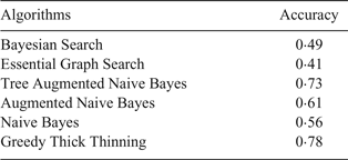
With this background in mind, we performed a BN analysis. For comparison of the different BN models, the specifications given in Section 2.2 have been followed (six models; five-fold cross-validation with 1,000 repetitions; accuracy and AUC comparison). We define a binary outcome with only two events to be observed: Rwy80 < 2, 500 and Rwy80 ≥ 2, 500. As in this database there are very few cases under the recommendation of the Flight Safety Foundation; we will try to identify landings not only under 2,000 feet, but also close to them (<2,500). This is intended to make the requirement stricter. Table 7 lists the accuracies of the six algorithms after cross-validation. The Greedy Thick Thinning algorithm has the greatest accuracy (0·78), followed by the Tree Augmented Naive Bayes (0·73).
Accuracies for the six algorithms evaluated

ROC curves present a false positive rate (one-specificity) versus sensitivity. The area under the ROC curve (AUC) is a measure of performance used for classification models. It is the most used performance metric together with accuracy rate.
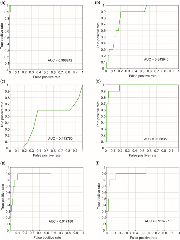
Figure 3 presents the ROC curves and AUCs for the six algorithms following the cross-validation procedure. Again, the best performance was for the Greedy Thick Thinning algorithm (AUC = 0 · 998), followed by the Tree Augmented Naive Bayes (AUC = 0 · 968).
ROC curves and AUCs using different algorithms for Rwy < 2,500: (a) Greedy Thick Thinning; (b) Bayesian Search; (c) Essential Graph Search; (d) Tree Augmented Naive Bayes; (e) Augmented Naive Bayes; (f) Naive Bayes.

Given that it had the best results, the Greedy Thick Thinning algorithm was run to construct the final BN used. The space of states for Rwy80 was then divided into six intervals: <2,500, [2,500, 3,000), [3,000, 3,500), [3,500, 4,000), [4,000, 4,500), ≥4,500.
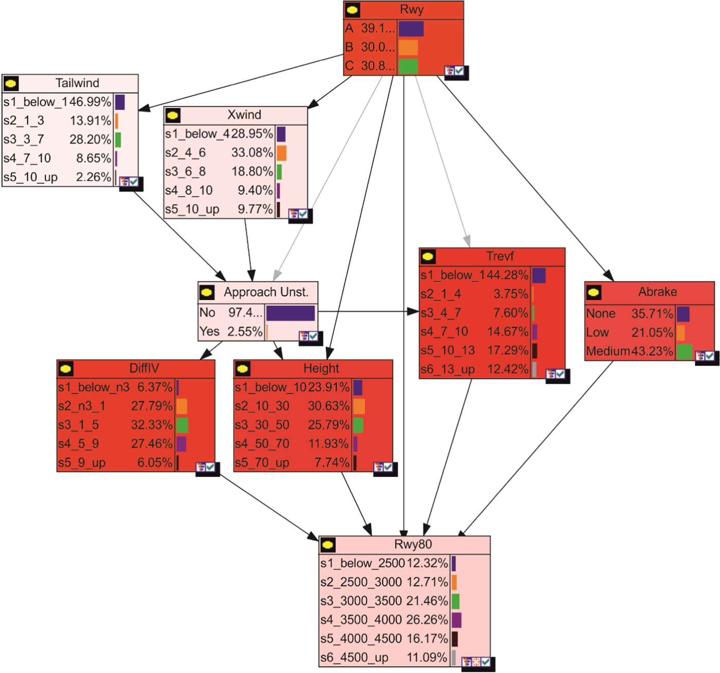
The estimated marginal probabilities in the BN (in the form of percentages) associated with each state are presented for each node in Figure 4. Relationships are represented by arcs, for which aviation experts checked that the connections represented were meaningful.
Graphical representation of the BN considered.

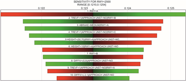
We performed a sensitivity analysis to observe if small changes in the predictors have an important effect on the prediction of the feature measuring the runway remaining at 80 knots. In Figure 4, the nodes are shown in a graduated red colour so that the more intense the colour, the greater influence this variable has on the conditional probability of the target node (Rwy80): runway, height at threshold, speed difference, autobrake activation and maximum reverse thrust seem the most influential variables. Figure 5 provides a tornado chart with which to analyse the influence of each state on the target variable, showing the ten most relevant states or state combinations. In particular, the figure shows the changes in P[Rwy80 < 2, 500] when varying the probability of the states shown at each bar by ±20%. Green denotes an increase of 20%, whereas red denotes a decrease of 20%. For instance, considering the top bar, if the probability of landing on Runway A increases by 20%, then P[Rwy80 < 2, 500] rises to 0·125. On the other hand, if the probability of landing on Runway A decreases by 20%, then P[Rwy80 < 2, 500] declines to 0·121. Although, at first sight, this might seem a rather small probability difference, it implies four more accidents per 1,000 operations. Since aviation accident rates tend to be very low, this could be a major point of analysis to bear in mind so as to try to reduce even small risks.
Tornado chart for the less than 2,500 feet of runway remaining at 80 knots event.

We then constructed ten risk scenarios using evidence propagation. This allowed us to evaluate the risk of overrun based on hypothetical scenarios with the states of the variables of interest considered. For each scenario, a probability of 1 (100% in percentage terms) is set for one state in one or more nodes.
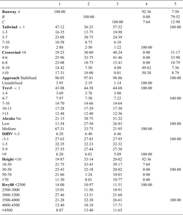
Firstly, three scenarios were defined to analyse the characteristics of each runway as represented by the data and two further scenarios were formulated to describe situations with maximum and minimum runway overrun risks. Table 8 presents the results of the inference process based on the BN considered.
Scenarios for excursion risk evaluation by runway

Comparing the first three scenarios related to runways, we observe that Runway A has the greatest percentages of landings with more than 10 knots of tailwind (2·88%) and crosswind (17·31%) and Runway C the lowest. Runway A also stands out in unstabilised landings (3·95%), followed by 2·19% for Runway B and 1·14% for Runway C. The activation time for maximum reverse thrust is similar for the three runways. The use of autobrake systems is very different, however, with Runway A requiring the greatest activation of autobraking at a medium level (67·31%) and Runway B the least (21·95%). The recommendation is that these two braking systems should be used moderately during landing roll. Runway B has the greatest percentage of moderate use of both devices. According to all this information, Runway A could be catalogued as riskier, and landings should be taken more carefully, for example, when situations with high wind are observed.
Speed difference is similar for the three runways. Nevertheless, for differences greater than 9 knots, Runway A presents a slightly greater percentage than B and C. Height at threshold differs considerably among the three runways. Again, Runway A has the greatest percentage (32·96%) of landing manoeuvres at threshold above the recommended height of 50 feet. Runway C has a percentage of 20·78%, while Runway B is the safest in this regard with 1·24%. In this case runway A should have stricter recommendations for landing for the speed and the height at the threshold.
With respect to the remaining length of runway at 80 knots, Runway A has the greatest percentage (14%) of lengths being less than 2,500 feet, followed by Runway C with 11·51% and finally by Runway B with 10·97%. Considering the accumulated percentages for landings with more than 3,500 feet remaining, we observe that Runway B would be the safest with 63·96%, followed by Runway C with 55·97%, and, finally, Runway A with 43·55%.
This analysis by runway is an example of the valuable insights that could be offered to any airport, giving the main risks to be observed during landing. Each different runway has its own characteristics and risks. A customised probability of suffering accidents could be given for any different runway.
We next analyse the scenarios for maximum and minimum risks, according to the FSF's recommendations. Scenario 4 considers conditions not recommended for landing by the FSF. This kind of landing has most probability of occurring at Runway A (92·36%), whereas at Runway C it would be 7·64%. According to the BN model, these conditions would be rarely met at Runway B. The opposite is the case for Scenario 5, where the best landing conditions are considered. In this case, there is a probability of 79·52% that the landing was performed on Runway B, followed by Runway C (12·98%) and with the lowest probability being for Runway A (7·5%).
All the information provided in the scenarios in Table 8 is coherent with the statement that Runway B is the safest, followed by Runway C, and, finally, with Runway A being the least safe. This also agrees with the results obtained in Section 3.1.
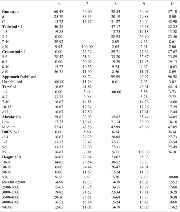
Five additional relevant scenarios not compliant with some of the most common FSF recommendations are presented in Table 9. Scenario 6 analyses the probability of an unstabilised approach. Runway A has the greatest percentage of unstabilised approaches (60·48%), whereas Runway B has almost double the percentage of Runway C (25·79% vs 13·79%). When the approach is unstabilised, 56·31% of the landings are performed with a crosswind greater than 10 knots (much greater than in the rest of the scenarios). Also, the speed difference is greater than 9 knots for 16·67% of the landings, a larger value than for the other scenarios. Autobrake systems are mainly used at a medium level (52·43%). Finally, 14·98% of the landings with an unstabilised approach had a remaining runway length at 80 knots of less than 2,500 feet, showing the risk of unstabilised approaches for a runway overrun.
Scenarios to evaluate runway excursion risk that are non-compliant with FSF recommendations

In Scenario 7, tailwind speed was considered to be greater than 10 knots. This situation occurs above all on Runway A (50%), followed by Runway B (33·33%). Although crosswind risk probabilities are not greatly affected by tailwinds greater than 10 knots, they do seem to be related to the stabilisation of the approach (11·26% of the approaches are unstabilised in this case). This scenario also shows the need to use autobraking at a medium level (for which the percentage is relatively high, 48·56%). A remaining length at 80 knots of less than 2,500 feet seems to be not especially affected by high tailwind speeds in comparison with the other scenarios.
Scenario 8 considers a case in which maximum reverse thrust is used briefly (between 1 and 4 seconds). This almost always occurs for stabilised approaches (99·9%). The probability of initiating landing with a height above 50 feet is 19·94%, the greatest value in these scenarios. Finally, the probability of having less than 2,500 feet remaining length on the runways at 80 knots is 14·79%, one of the greatest probabilities of the scenarios analysed.
A large difference between recommended and actual speeds can lead to considerable risk during landing. Scenario 9 considers the consequences associated with a speed difference larger than 9 knots. Again, this risky situation most probably occurs at Runway A (40·08%), followed by Runways B and C with 29·88% and 30·04%, respectively. Speed differences greater than 9 knots occur with a probability of 7·03% in unstabilised approaches. The worst consequence is that the probability of landing with a remaining runway length of less than 2,500 feet at 80 knots is 15·05%.
Scenario 10 is related to heights greater than 70 feet at threshold. This kind of situation appears to be almost improbable for the landings on Runway B, whereas the probabilities for Runways A and C are 57·1% and 42·9%, respectively. In this case, a landing that is initiated at a greater than normal height seems to be not associated with other negative factors. Moreover, the probability of a remaining runway length at 80 knots that is less than 2,500 feet is the lowest (12·52%) of the risk scenarios in Table 9.
In summary, on one hand, an unstabilised approach and a large speed difference constitute two major factors for unsafe landings. When an approach is unstabilised, it is typically accompanied by some non-recommended conditions, for example, high crosswind and tailwind speeds, or a large speed difference. Both unstabilised approaches and high-speed differences occur with greater frequency at Runway A. On the other hand, for the probability of having a remaining runway length of less than 2,500 feet at 80 knots, the least dangerous factors are tailwind speed and height. Having all these aspects under control can lead to a safer context, reducing runway excursion incident rates.
Finally, evidence propagation in the BN has allowed us to define risk scenarios that provide information about hypothetical situations that could arise in real landings. The method is extensible to other aviation datasets. Indeed, in general, the more data, the better the information that would be obtained.
4. CONCLUSIONS
This paper explores the risk for runway overrun excursions under several scenarios. Data from three real runways were collected and analysed with a BN model, as an illustration of a risk evaluation that could be performed for all runways. The BN method using evidence propagation facilitated the analysis of the most common runway excursion risk scenarios.
This research revealed the relations among features measured when landing. Three runways were classified in accordance with their potential risks, and early risk disclosure was provided. The generic recommendations established by safety organisations can be revisited for each runway using the results of this type of analysis. For example, Runway A is less safe than the others, and recommendations for landing should be stricter. This kind of analysis can be performed for more runways in different airports, providing a classification according to their runway overrun risk. This tool could be used in aviation operations for runway classification that allows pilots to have a runway excursion probability when landing.
The proposed approach can provide insights into why runway excursions occur and potentially lead to reductions in accident rates. The runway risk ranking could be useful for authorities to mitigate the number of excursions, improving the weaknesses observed at each runway. With the BN graph, the scenarios given and the sensitivity analysis, the relations and influence between the main features is exposed. These results could be extended if more airports open their databases. This study remains open in case further data can be obtained in the future. New features such as touchdown point, landing procedure, weather situation or runway contamination would be especially important. The results obtained cover different kinds of risk, offering a comprehensive safety framework that would be applicable to all runways.
FINANCIAL SUPPORT
This research was supported by the Agencia Estatal de Investigación - Spain (Projects MTM2014-56949-C3-3-R and MTM2017-86875-C3-2-R); the Gobierno de Extremadura - Spain (Projects GR15106 and GR18108); and the European Union (European Regional Development Funds).