2.1. Description of the mathematical model of unmanned sailboat

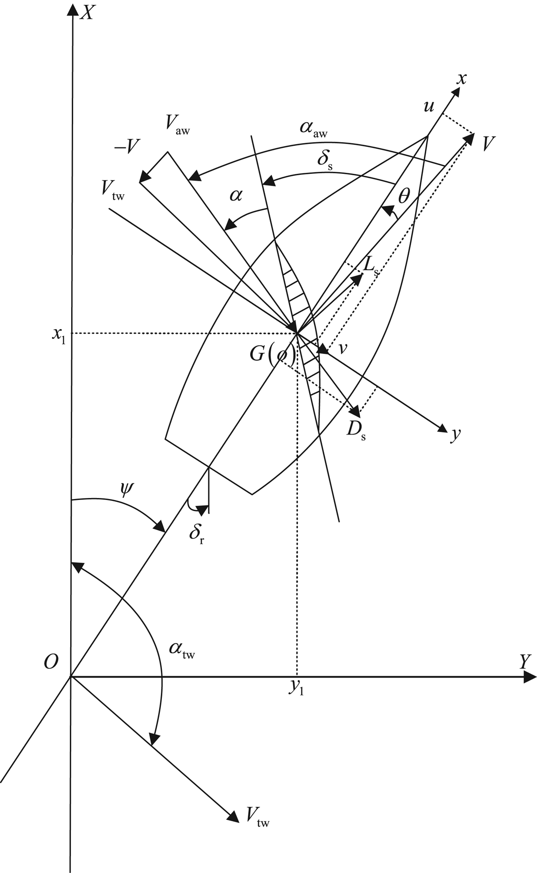
The earth-fixed reference frame $XOY$ and body-fixed reference frame $xoy$ are shown in Figure 1. The coordinate origin $O$ is the starting position of the unmanned sailboat, and the axes $OX$ and $OY$ point to the north and east, respectively; the coordinate origin $o$ is the centre of gravity of the unmanned sailboat $G(o)$, the axis $ox$ is directed from aft to fore and $oy$ points to starboard. As shown in Figure 1, in the body-fixed reference frame, with the magnitude of the apparent wind ${V_{\rm aw}}$ and direction ${\alpha_{\rm aw}}$, ${\delta _{\rm s}}$ is the sail angle, $\alpha$ represents the sail angle of attack and the leeway angle is $\theta$. These satisfy the formula ${\delta _{\rm s}}={\alpha_{\rm aw}}-\alpha -\theta$. The actual sailing speed is represented by $V$. It can be divided into the surge velocity $u$ and the sway velocity $v$ on different axes, and they satisfy the formula ${V^{2}} = {u^{2}} + {v^{2}}$. The ${L_{\rm s}}$ and ${D_{\rm s}}$ are the sail lift and drag forces, and the rudder angle is represented by ${\delta _{\rm r}}$. In the earth-fixed reference frame, ${V_{\rm tw}}$ is the magnitude of the true wind and ${\alpha _{\rm tw}}$ its direction. The position of the sailboat is represented by (${x_1}$, ${y_1}$). The heading (yaw) angle of the unmanned sailboat is $\psi$, which represents the angle from the axis $ox$ to $OX$.

Figure 1.

Reference coordinate frames of the unmanned sailboat

Xiao and Jouffroy (Reference Xiao and Jouffroy2014) described the kinematics and kinetics equations of an unmanned sailboat. On this basis, we add disturbances such as waves or wind, so that a 4-DOF unmanned sailboat dynamic model is established as follows:

(1)\begin{equation} \left\{\begin{aligned} {\dot x} & = u\cos \psi - v\sin\psi \cos\phi \\ {\dot y} & = u\sin \psi + v\cos\psi \cos\phi \\ \dot \phi & = p\\ \dot \psi & = r\cos \phi \\ \dot u & =( {( {m - {Y_{\dot v}}} )vr - {F_{xk}} - {F_{xh}} + {F_{xs}} + {F_{xr}} + {X_{\rm wave}}})\\ & \quad \times {( {m - {X_{\dot u}}} )^{ - 1}}\\ \dot v & = ( {( { - m + {X_{\dot u}}} )ur - {F_{yk}} - {F_{yh}} + {F_{ys}} + {F_{yr}} + {Y_{\rm wave}}} )\\ & \quad\times {( {m - {Y_{\dot v}}} )^{ - 1}}\\ \dot p & = ( - {M_r}( \phi ) - {M_{xk}} - {M_{xh}} + {M_{xs}} + {M_{xr}} - {M_{\phi d}}(\dot \phi )\\ & \quad + {K_{\rm wave}}){({I_{xx}} - {K_{\dot p}})^{ - 1}}\\ {\dot r} & = (( - {X_{\dot u}} + {Y_{\dot v}})u\nu - {M_{zk}} - {M_{zh}}+{M_{zs}} + {M_{zr}}\\ & \quad - {M_{\psi d}}(\dot \psi )\cos \phi + {N_{\rm wave}}){({I_{zz}} - {N_{\dot r}})^{ - 1}} \end{aligned}\right. \end{equation}

where $p$, $\phi$ and $r$ denote the roll velocity, the roll angle and the yaw velocity, respectively; ${F_{x\cdot }}$, ${F_{y\cdot }}$, ${M_{x\cdot }}$, ${M_{z\cdot }}$ are the forces and moments of different parts; and $s$, $r$, $k$ and $h$ represent the sail, rudder, keel and hull of the unmanned sailboat, respectively. Here, ${M_{\phi d}}(\dot \phi )$, ${M_{\psi d}}(\dot \psi )$ and ${M_r}( \phi )$ denote the heel-damping matrix, the yaw-damping matrix and the static-righting moment, respectively; ${I_{xx}}$ and ${I_{zz}}$ are the principle moment of inertia on $x$ and $z$; and ${X_{\dot u}}$, ${Y_{\dot v}}$, ${K_{\dot p}}$, ${N_{\dot r}}$ represent the added mass coefficients. These formulae are detailed by Xiao and Jouffroy (Reference Xiao and Jouffroy2014). In (1), ${X_{\rm wave}}$, ${Y_{\rm wave}}$, ${K_{\rm wave}}$, ${N_{\rm wave}}$ denote the force and moment produced by wave disturbances as follows:

\[ \left\{ \begin{aligned} {X_{\rm wave}} & = 2aB\displaystyle\frac{{\sin b \sin c}}{c}\varepsilon (t) \\[3pt] {Y_{\rm wave}} & =2aL\displaystyle\frac{{\sin b\sin c}}{b}\varepsilon \left( t \right)\\[3pt] {K_{\rm wave}} & = \displaystyle\frac{1}{2}{\rho_{\rm ater}}gm{h_c}k{A_a}\sin\mu \,e^{{-}kT/2}\sin {\omega_e}t\\[3pt] {N_{\rm wave}} & = ak\left( {B^{2}}\sin b\displaystyle\frac{{c\cos c - \sin c}}{{{c^{2}}}}{- {L^{2}}\sin c\displaystyle\frac{{b\cos b - \sin b}}{{{b^{2}}}}} \right)\xi (t) \end{aligned}\right. \]

where $m$, $L$, $B$ and ${A_a}$ represent the mass, length, width and the sail area of the unmanned sailboat; $T$ and $k$ are the draft and the wavenumber; $\rho _{{\rm water}}$ and $g$ are the density of seawater and the acceleration of gravity; ${h_c}$, $\mu$ and ${\omega _e}$ denote the initial meta-centric height, the wave direction angle and the encounter frequency, respectively. Among them, $a = \rho _{{\rm water}}g( 1 - e^{ - kT} )/k^{2}$, $b = ( kL/2 )\cos \mu$, $c = ( {kB/2} )\sin \mu$, $\xi ( t ) = ( {h/2} )\cos ( \omega _e t )$, $\varepsilon ( t ) = ( {kh/2} )\sin ( {{\omega _e}t} )$, and $h$ is the significant wave height.

2.2. Problem formulation

From the 4-DOF unmanned sailboat dynamic model (1), we can get the mathematical model of the sailing speed,

(2)\begin{equation} \dot u = f(u,v,p,r,{\delta_s}), \end{equation}

where

\[ f = ((m - {Y_{\dot v}})vr - {F_{xk}} - {F_{xh}} + {F_{xs}} + {F_{xr}} + {X_{\rm wave}}){(m - {X_{\dot u}})^{ - 1}}. \]

When studying the ESC optimisation scheme, if the input and output of the optimised object are known, we can approximate the optimised object to a general nonlinear system. So the model (2) can be written as

(3)\begin{equation} \begin{aligned} \boldsymbol{{\dot x}} & =\boldsymbol{f}(\boldsymbol{x},{\delta_s}),\\ u & = h(\boldsymbol{x}), \end{aligned} \end{equation}

where $f$ and $h$ both are smooth functions representing the system state and output equation, and $\boldsymbol {x} \in \boldsymbol{R^{n}}$, ${\delta _s} \in \boldsymbol{R}$ and $u \in \boldsymbol{R}$ denote the system state, input and output.

The sail angle control law is

(4)\begin{align} {\delta_s} & = {\alpha_{\rm aw}} - ({\alpha_0} + {\delta_\alpha })\nonumber\\ & = \alpha (\boldsymbol{x},{\delta_\alpha }), \end{align}

where ${\alpha _0}$ and ${\delta _\alpha }$ represent the sail angle of attack and optimal sail angle of attack, respectively. Inserting (4) into (3), we get

(5)\begin{equation} \boldsymbol{\dot x} = \boldsymbol{f}(\boldsymbol{x},\alpha (\boldsymbol{x},{\delta_\alpha })). \end{equation}

Some assumptions are as follows:

Assumption 3 There is $\delta _\alpha ^{*} \in R$ such that

\begin{align*} u' & = {(h \circ l)^{\prime} }(\delta_\alpha^{*})= 0,\\ u''& = {(h \circ l)^{\prime \prime }}(\delta_\alpha^{*})< 0. \end{align*}

It guarantees that $u = h(l({\delta _\alpha }))$ can obtain the optimal speed at the optimal value $\delta _\alpha ^{*}$.

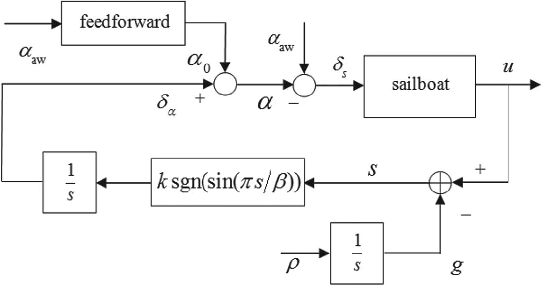
Assumption 4 In Figure 2, the adjustment rate of ${\delta _\alpha }$ determined by the ESC scheme is much slower than the system dynamic, and the system dynamic in (3) refers to the dynamic from ${\delta _\alpha }$ to cost function $u(t)$. So to analyse the sliding mode more conveniently and simply, we ignore this dynamic at first, so the cost function $u(t) = h(\boldsymbol {x}(t))$ can be approximated by

(6)\begin{equation} u(t) = h(l({\delta_\alpha }(t))) \buildrel \Delta \over = H({\delta_\alpha }(t)). \end{equation}

Figure 2.

SMESC speed optimisation scheme

To sum up, the control objective is: under the above assumptions for the controlled object (5), ${\delta _\alpha }$ achieves the tracking of $\delta _\alpha ^{*}$ in the process of optimisation, so that $u$ reaches the maximum speed.

3.1. Basic principles

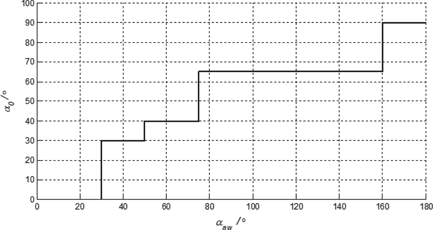
As shown in Figure 2, the speed optimisation scheme includes the feedforward part and the SMESC feedback part. The main function of this feedforward part is to avoid a large deviation between $u$ and the optimal value. The ${\alpha _0}$ is first computed by a piecewise constant function. As shown in Figure 3, the piecewise constant function is obtained by a rough fitting based on the speed polar diagram information. The basic principle is to adjust $\alpha$ based on different ${\alpha_{\rm aw}}$ to produce the optimal ${F_{xs}}$ and $u$.

Figure 3.

Offline calculation of ${\alpha _0}$

For the feedback control, the basic idea is to devise the sliding mode control law ${\dot \delta _\alpha }=k\,{\rm sgn}(\sin (\pi s /\beta ))$. During the sliding mode motion, no matter how the gradient of the function changes, $H({\delta _\alpha }(t)) - g(t)$ will be kept as a constant, then $H({\delta _\alpha }(t))$ will be forced at the same rate as $\rho$ increases with $g(t)$. After the sliding mode extremum seeking feedback control, an ${\delta _\alpha }$ is generated, and the actual $\alpha$ is obtained by combining ${\alpha _0}$ and ${\delta _\alpha }$. The actual control of an unmanned sailboat is ${\delta _s}$, not $\alpha$, where ${\delta _s}$ is obtained from the formula ${\delta _s} = {\alpha_{\rm aw}} - \alpha$. The closed-loop control is formed by ${\delta _s}$ acting on the controlled object. After feedback optimisation of the SMESC, $u$ reaches the maximum speed value. However, due to the structural performance of SMESC, it has steady-state oscillation.

3.2. The analysis of sliding modes

The SMESC speed optimisation scheme is shown in Figure 2. The switching function $s(t)$ is defined as

(7)\begin{equation} s(t) = u(t) - g(t), \end{equation}

where $g(t)$ is monotonically increasing and $\dot g(t) = \rho$ is positive. Here, ${\dot \delta _\alpha }$ satisfies

(8)\begin{equation} {\dot \delta_\alpha } = k \,{\rm sgn}(\sin (\pi s/\beta)), \end{equation}

where $k$, $\beta$ are both positive, and the derivative of $s(t)$ is

(9)\begin{align} \frac{d}{{dt}}s(t)& = \dot u(t) - \dot g(t) = \displaystyle\frac{d}{{d{\delta_\alpha }}}H({\delta _\alpha }){{\dot \delta }_\alpha } - \dot g(t)\nonumber\\ & = \Phi ({\delta_\alpha }) k\, {\rm sgn}(\sin (\pi s(t)/\beta)) - \rho, \end{align}

where $\Phi ({\delta _\alpha }) = ({d}/{{d{\delta _\alpha }}})H({\delta _\alpha })$ is the derivative of $H({\delta _\alpha })$ to ${\delta _\alpha }$.

If a constant $c$ makes

\[ (s(t) - c)\displaystyle\frac{d}{{dt}}(s(t) - c) < 0 \]

true, the sliding mode occurs at $s(t) = c$. The surge velocity $u(t)$ increases with the increasing of $g(t)$, and the optimal ${\delta _\alpha }$ moves towards the maximum $\delta _\alpha ^{*}$.

Next, a more rigorous and concise method is used to analyse the sliding modes compared with the analysis method of Pan et al. (Reference Pan, Qzguner and Acarman2003).

According to the sliding mode control law (8) and trigonometric function,

\[ \sin (\pi s(t)/\beta) = 2\sin (\pi s(t)/2\beta)\cos (\pi s(t)/2\beta), \]

the corresponding switching function is defined as

(10)\begin{equation} \begin{aligned} {\Gamma_l}(t) = \sin (\pi s(t)/2\beta),\\ {\Gamma_r}(t) = \cos (\pi s(t)/2\beta). \end{aligned} \end{equation}

It can be seen that the corresponding sliding modes are

(11)\begin{equation} \frac{{s(t)}}{\beta } = \begin{cases} 2n & \Gamma_l(t) = 0,\\ 2n + 1 & \Gamma_r(t) = 0, \end{cases}\end{equation}

where $n = 0, \pm 1, \pm 2\ldots$.

First, analysing ${\Gamma _l}(t)$ and the derivative of ${\Gamma _l}(t)$ gives

(12)\begin{equation} {\dot \Gamma_l}(t) = \frac{\pi }{{2\beta }}\cos (\pi s(t)/2\beta)\frac{d}{{dt}}s(t), \end{equation}

so

(13)\begin{equation} {\Gamma_l}(t){\dot \Gamma_l}(t) = \frac{\pi }{{4\beta }}\sin (\pi s(t)/\beta) (\Phi ({\delta_\alpha }) k \,{\rm sgn}(\sin (\pi s(t)/\beta)) - \rho). \end{equation}

From (13), we can get the following conclusions:

1. (1) Under $\sin (\pi s(t)/\beta ) > 0$ ($2n < s(t)/\beta < 2n + 1$) and $\Phi ({\delta _\alpha }) < {\rho }/{k}$, ${\Gamma _l}(t){\dot \Gamma _l}(t) < 0$ holds. Because of $\dot s(t) = \Phi ({\delta _\alpha }) k \,{\rm sgn}(\sin (\pi s(t)/\beta )) - \rho$, $\dot s(t) < 0$ is known, so $s(t)/\beta \to 2n$.

2. (2) Under $\sin (\pi s(t)/\beta ) < 0$ ($2n + 1 < s(t)/\beta < 2n + 2$) and $\Phi ({\delta _\alpha }) < - {\rho }/{k}$, ${\Gamma _l}(t){\dot \Gamma _l}(t) < 0$ holds, $\dot s(t) > 0$ is known, so $s(t)/\beta \to 2n + 2$.

The same analysis of ${\Gamma _r}(t)$ gives

(14)\begin{align} {\dot \Gamma_r}(t)& ={-} \frac{\pi }{{2\beta }}\sin (\pi s(t)/2\beta)\frac{d}{{dt}}s(t), \end{align}

(15)\begin{align} {\Gamma_r}(t){\dot \Gamma_r}(t)& ={-} \frac{\pi \sin (\pi s(t)/\beta)}{{4\beta }} (\Phi ({\delta_\alpha }) k \,{\rm sgn}(\sin (\pi s(t)/\beta)) - \rho ). \end{align}

From (15), we can get the following conclusions:

1. (1) Under $\sin (\pi s(t)/\beta ) > 0$ ($2n < s(t)/\beta < 2n + 1$) and $\Phi ({\delta _\alpha }) > {\rho }/{k}$, ${\Gamma _l}(t){\dot \Gamma _l}(t) < 0$ holds. Because of $\dot s(t) = \Phi ({\delta _\alpha }) k \,{\rm sgn}(\sin (\pi s(t)/\beta )) - \rho$, $\dot s(t) > 0$ is known, so $s(t)/\beta \to 2n + 1$.

2. (2) Under $\sin (\pi s(t)/\beta ) < 0$ ($2n + 1 < s(t)/\beta < 2n + 2$) and $\Phi ({\delta _\alpha }) > - {\rho }/{k}$, ${\Gamma _l}(t){\dot \Gamma _l}(t) < 0$ holds, $\dot s(t) < 0$ is known, so $s(t)/\beta \to 2n + 1$.

Unlike simple sliding mode control, which has only a single sliding mode, SMESC has a series of sliding modes that ensures a sliding mode is achieved regardless of the initial state of the system. Through the above analysis, a series of sliding modes of SMESC is drawn, as shown in Figure 4.

Figure 4.

SMESC convergence process and sliding modes

Figure 4 shows the convergence process of the optimisation system, which consists of three phases:

1. A. The convergence phase – the system from the initial position converges to the nearest sliding mode.

2. B. The forced tracking phase – after reaching a sliding mode, the system is forced to track a preset reference signal and gradually converges to the neighbourhood of an extremum point, i.e. $\Phi ({\delta _\alpha }) \in ( -\rho /k,\rho /k)$.

3. C. The steady-state oscillation phase – it will maintain steady-state oscillation near the extremum point.

3.3. The stability analysis

First, the system is analysed from the initial position to the sliding mode and defines a $\delta$ neighbourhood of the extremum point $\delta _\alpha ^{*}$ as

(16)\begin{equation} {\Theta_{({\delta_l},{\delta_r})}}=\{ {{\delta_\alpha }} \,|\,\delta_\alpha^{*} - {\delta_l} \le {\delta_\alpha } \le \delta_\alpha^{*} + {\delta_r}\}, \end{equation}

where ${\delta _l}$ and ${\delta _r}$ are positive constants and satisfy

(17)\begin{align} | {\Phi ({\delta_\alpha })} | & > \frac{\rho }{k},\quad \forall {\delta_\alpha } \notin {\Theta_{({\delta_l},{\delta_r})}}, \end{align}

(18)\begin{align} | {\Phi ({\delta_\alpha })} | & \le \frac{\rho }{k},\quad \forall {\delta_\alpha } \in {\Theta_{({\delta_l},{\delta_r})}}, \end{align}

(19)\begin{align} | {\Phi ({\delta_\alpha })} | & = \frac{\rho }{k} \Leftrightarrow {\delta_\alpha } = \delta_\alpha^{*} - {\delta_l} \text{ or } {\delta_\alpha } = \delta_\alpha^{*} + {\delta_r}. \end{align}

Based on the analysis of the sliding mode in the previous section, it can be seen that when $\Phi ({\delta _\alpha }) < - {\rho }/{k}$, ${\Gamma _l}(t){\dot \Gamma _l}(t) < 0$ is established, and the system converges to sliding mode ${\Gamma _l}(t) = 0$; when $\Phi ({\delta _\alpha }) > {\rho }/{k}$, ${\Gamma _r}(t){\dot \Gamma _r}(t) < 0$ is established, and the system converges to ${\Gamma _r}(t) = 0$. That is, for any initial state ${\delta _\alpha }(0)$ of the system, as long as parameters $k$ and $\rho$ are selected to satisfy

(20)\begin{equation} | {\Phi ({\delta_\alpha }(0))} | \gg \frac{\rho }{k},\quad {\delta_\alpha}(0) \notin {\Theta_{({\delta_l},{\delta_r})}} \end{equation}

then

(21)\begin{equation} {\Gamma_l}(t){\dot \Gamma_l}(t) < 0\quad \text{or}\quad {\Gamma_r}(t){\dot \Gamma_r}(t) < 0 \end{equation}

will exist. The system converges to ${\Gamma _l}(t) = 0$ or ${\Gamma _r}(t) = 0$.

Next, the convergence of the optimisation system in sliding mode (phase II) will be analysed. The equivalent control theory is applied, the sliding mode control law is written

(22)\begin{equation} \begin{aligned} {{\dot \delta }_\alpha } & = \mu, \\ \mu & = k \,{\rm sgn}(\sin (\pi s(t)/\beta)). \end{aligned} \end{equation}

Let

(23)\begin{equation} \frac{d}{{dt}}\sin (\pi s(t)/\beta)=0, \end{equation}

the equivalent control input in the sliding modes $s(t) = n\beta$ can be obtained

(24)\begin{equation} {\mu_{eq}} = {\dot \delta_\alpha } = \frac{\rho }{{\Phi ({\delta_\alpha })}}. \end{equation}

It is known that $\delta _\alpha ^{*}$ is a maximum point, $({\delta _\alpha }- \delta _\alpha ^{*})\Phi ({\delta _\alpha }) < 0$ when ${\delta _\alpha } \ne \delta _\alpha ^{*}$, and we get

(25)\begin{equation} ({\delta_\alpha }-\delta_\alpha^{*})\frac{d}{{dt}}({\delta_\alpha }-\delta_\alpha^{*}) = ({\delta_\alpha }-\delta_\alpha^{*})\frac{\rho }{{\Phi ({\delta_\alpha })}} < 0. \end{equation}

In summary, the optimisation system gradually converges to the maximum value of the sliding mode.

Finally, we analyse the III phase. After the system converges to $| {\Phi ({\delta _\alpha })}| \le {\rho }/{k}$, sliding modes disappear and there is

(26)\begin{equation} \dot s(t) = \Phi ({\delta_\alpha }) k \,{\rm sgn}(\sin (\pi s(t)/\beta)) - \rho < 0. \end{equation}

Supposing the optimisation system converges to $| {\Phi ({\delta _\alpha })}| \le {\rho }/{k}$ in mode $s(t)=(2n + 1)\beta$, there are

(27)\begin{align} & 2n\beta < s(t) < (2n + 1)\beta, \end{align}

(28)\begin{align} & {\dot \delta_\alpha }= k\, {\rm sgn}(\sin (\pi s(t)/\beta))=k > 0, \end{align}

where ${\delta _\alpha }$ keeps going up, and two cases may occur.

Case 1: If the design of ${\rho }/{k}$ is small, the system will pass through $| {\Phi ({\delta _\alpha })} | \le {\rho }/{k}$ to reach $| {\Phi ({\delta _\alpha })} | > {\rho }/{k}$ before $s(t)$ reduces to $2n\beta$. In this region, the sliding modes condition is established, the system converges to $s(t) = 2n\beta$ and moves to $| {\Phi ({\delta _\alpha })} | \le {\rho }/{k}$ after reaching the sliding mode, and we get

(29)\begin{align} & (2n - 1)\beta < s(t) < 2n\beta, \end{align}

(30)\begin{align} & {\dot \delta_\alpha }= k \,{\rm sgn}(\sin (\pi s(t)/\beta ))={-} k < 0. \end{align}

Now ${\delta _\alpha }$ continues to decrease until after the system converges to $s(t)=(2n - 1)\beta$, the system is going to move in the opposite direction, and ${\delta _\alpha }$ keeps going up. The system is going to repeatedly move around the maximum point $\delta _\alpha ^{*}$, forming a large steady-state oscillation, as shown by the red trajectory in Figure 4.

Case 2: If the design of ${\rho }/{k}$ is large, the system is always in $| {\Phi ({\delta _\alpha })} | \le {\rho }/{k}$ when $s(t)$ reduces to $s(t) = 2n\beta$. Then (29) and (30) are established, and the motion direction of ${\delta _\alpha }$ reverses. When (27) and (28) are established, the motion direction of ${\delta _\alpha }$ reverses again. The system will repeatedly move around the maximum point $\delta _\alpha ^{*}$, forming a smaller steady-state oscillation, as shown by the pink trajectory in Figure 4. Therefore, the convergence of the SMESC speed optimisation system has been proved.

4.1. Basic principles

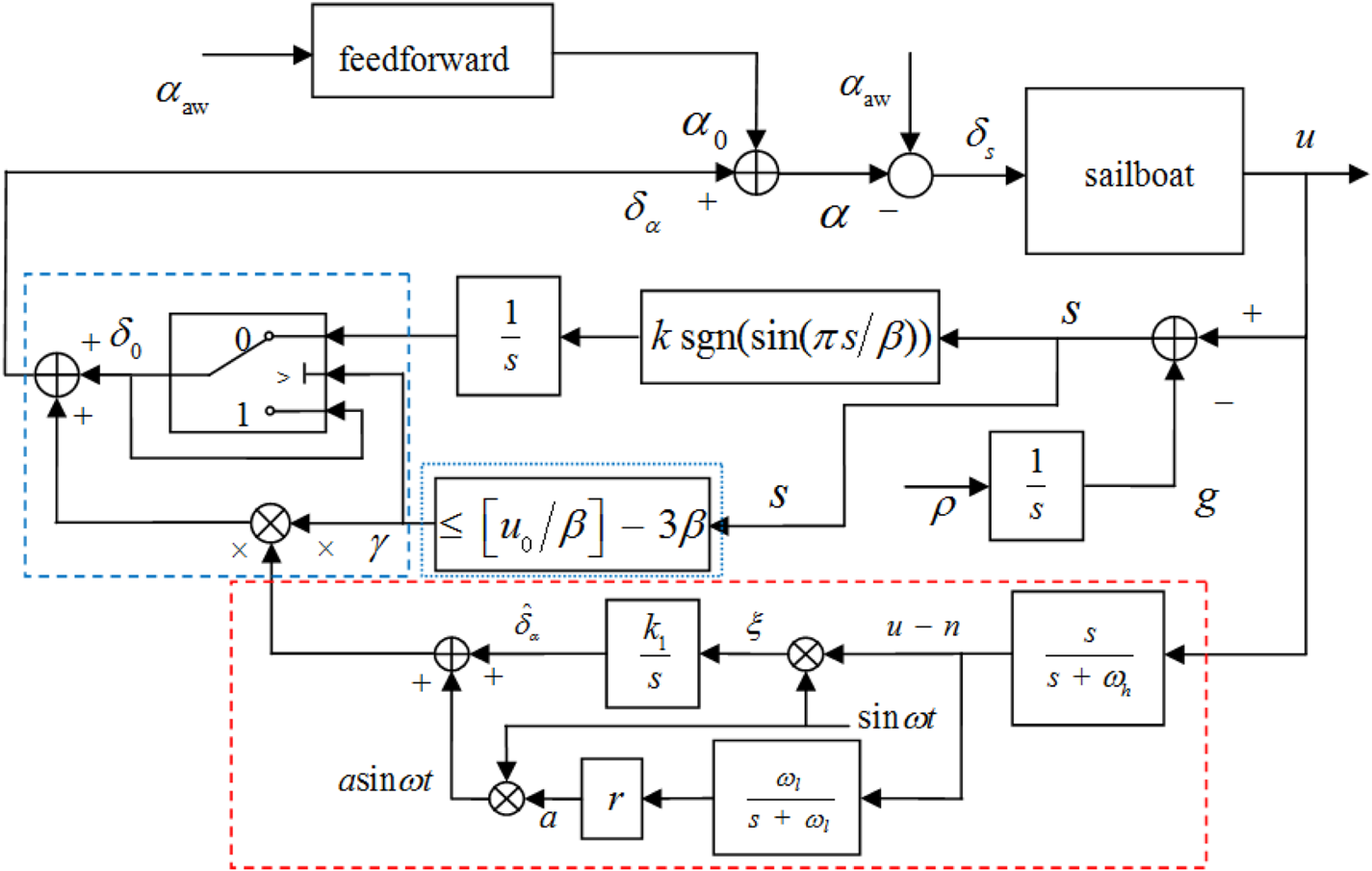
Based on the idea of switching between algorithms, by designing a switching law to combine SMESC with ESC without steady-state oscillation, the improved speed optimisation scheme by SMESC without steady-state oscillation is proposed and shown in Figure 5.

Figure 5.

SMESC without steady-state oscillation speed optimisation

In Figure 5, the red dashed box is the ESC without steady-state oscillation, whose introduction and stability proof are detailed by Shen et al. (Reference Shen, Wang, Yu and Guo2019). The switching law consists of two parts: one is the blue dotted box part on the right side, which can detect the convergence state of SMESC. When a certain state satisfies the switching condition, the system switches from SMESC to ESC without steady-state oscillation; the other is the blue dashed box on the left, which is a value holder. When the switching condition is satisfied, the value holder starts to work, which ensures the stability of the switch. The key to complete this improved scheme is to design the switching law.

4.2. Design of the switching law

To make full use of the advantages of the convergence phase of SMESC, and to combine it with the steady-state phase of ESC without steady-state oscillation, the switch action should be designed at the end of the SMESC forced trace phase, i.e. phase II, and during the switching period, the ${\delta _\alpha }$ should not jump. First, the detection of the convergence phase of the SMESC will be stated in detail for the $s(t)$ signal at the initial time

(31)\begin{equation} {s_0} = {u_0} - {g_0}, \end{equation}

where ${s_0}$, ${u_0}$ and ${g_0}$ are initial values. Here, ${g_0}$ is zero, so

(32)\begin{equation} \frac{{{s_0}}}{\beta } = \frac{{{u_0}}}{\beta }. \end{equation}

For any initial value ${u_0}$, there are three possibilities where $s(t)$ converges to sliding modes, i.e. $[u_0/\beta ]$ and $[u_0/\beta ] \pm \beta$, and $[ \bullet ]$ represents the rounding function. When this optimisation system converges to $| {\Phi ({\delta _\alpha })} | < {\rho }/{k}$, the sliding mode disappears and there is

(33)\begin{equation} \dot s(t)= \Phi ({\delta_\alpha }) k \,{\rm sgn}(\sin (\pi s(t)/\beta)) - \rho < 0. \end{equation}

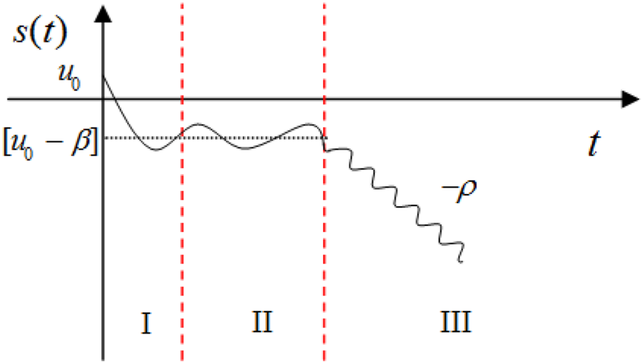
To sum up, the general trend of $s(t)$ is shown in Figure 6.

Figure 6.

The trend of $s(t)$

In Figure 6, first the signal $s(t)$ converges to the nearest sliding mode. After the end of the forced tracking phase, the SMESC enters the III phase and $s(t)$ changes significantly. So the signal $s(t)$ is used to determine whether the optimisation system has reached the steady-state oscillation phase. In summary, the threshold of the switching law can be set to $[u_0/\beta ] - \beta$, but to avoid the false switching caused by the sliding chattering, it is preferable to set the next sliding mode ($[u_0/\beta ] - 3\beta$) as a switch threshold, and obtain the conservative switching law

(34)\begin{equation} \gamma = \begin{cases} 0 & s(t) > [u_0/\beta] - 3\beta \\ 1 & s(t) \le [u_0/\beta] - 3\beta. \end{cases} \end{equation}

It can be known from (33) and (34) that only one switch is made in the optimisation process. The switching law includes two parts: the state judgment and value holder. When $s(t) > [u_0/\beta ] - 3\beta$, $\gamma = 0$, and the SMESC is working; when $s(t) \le [u_0/\beta ] - 3\beta$, $\gamma = 1$, ESC without steady-state oscillation starts to work. When the switching condition is satisfied, the value holder starts to work, which is used to maintain the estimated input value ${\delta _0}$ in SMESC. This is added to the optimisation system as the initial value of ESC without steady-state oscillation.

4.3. Stability analysis

Before carrying out the stability analysis of the entire optimisation system, the stability of the ESC without steady-state oscillation should be briefly introduced. The detailed stability proof has been analysed by Shen et al. (Reference Shen, Wang, Yu and Guo2019), and has led to the Theorem 1.

Based on the analysis of this entire optimisation scheme, Theorem 2 is obtained.

Proof. It is known that there is only one switching action in the SMESC without steady-state oscillation speed optimisation process. If SMESC is convergent and the ${\delta _\alpha }$ is in the convergence domain of ESC without steady-state oscillation after switching, this entire speed optimisation system is convergent.

The stability of SMESC has been proved in Section 3.3. Due to the choice of parameters, there are two cases in the steady-state oscillation phase. Considering the critical state in the two cases, that is, the variation range of $\Phi ({\delta _\alpha })$ is only $[- \rho / k, \rho /k]$, this system goes into $| {\Phi ({\delta _\alpha })} | \le {\rho }/{k}$ at ${t_0}$, and it gets to another boundary at ${t_1}$.

When $s(t)$ is $2n\beta < s(t) < (2n + 1)\beta$, there is

(35)\begin{align} & \Phi ({\delta_\alpha }({t_0})) = \frac{\rho }{k}, \quad \Phi ({\delta_\alpha }({t_1})) ={-} \frac{\rho }{k}, \end{align}

(36)\begin{align} & s({t_0}) - s({t_1}) ={-} \int_{{t_0}}^{{t_1}} {\dot s(t)} \,dt ={-} \int_{{t_0}}^{{t_1}} {(\Phi ({\delta_\alpha })} k - \rho )\,dt, \end{align}

where $\Phi ({\delta _\alpha }) \in [- \rho /k ,\rho /k]$, so $\dot s(t) \in [ - 2\rho ,0]$. Based on the Lagrange Mean Value Theorem, ${\bar s_1} \in ( - 2\rho ,0)$ is the mean of $\dot s(t)$, so

(37)\begin{equation} s({t_0}) - s({t_1}) ={-} \int_{{t_0}}^{{t_1}} {\dot s(t)} \,dt = {\bar s_1}({t_0} - {t_1}) \buildrel \Delta \over = \beta_1^{*} \end{equation}

is true.

When $s(t)$ is $(2n - 1)\beta < s(t) < 2n\beta$, there is

(38)\begin{align} \Phi ({\delta_\alpha }({t_0})) & ={-} \frac{\rho }{k},\quad \Phi ({\delta_\alpha }({t_1})) = \frac{\rho }{k}, \end{align}

(39)\begin{align} s({t_0}) - s({t_1})& ={-} \int_{{t_0}}^{{t_1}} {\dot s(t)} \,dt = \int_{{t_0}}^{{t_1}} {(\Phi ({\delta_\alpha })} k + \rho )\,dt, \end{align}

where $\Phi ({\delta _\alpha }) \in [- \rho /k,\rho /k]$, $\dot s(t) \in [ - 2\rho ,0]$. There is ${\bar s_2} \in ( - 2\rho ,0)$ such that

(40)\begin{equation} s({t_0}) - s({t_1}) ={-} \int_{{t_0}}^{{t_1}} {\dot s(t)} \,dt = {\bar s_2}({t_0} - {t_1}) \buildrel \Delta \over = \beta_2^{*} \end{equation}

holds. In summary, the following conclusion is obtained.

Consider the SMESC optimisation system. For $\rho /k > 0$, there is a positive ${\beta^{*}} = \min (\beta _1^{*},\beta _2^{*})$, such that for $\beta \in (0,{\beta^{*}})$, $\Phi ({\delta _\alpha })$ satisfies $| {\Phi ({\delta _\alpha })} | \le {\rho }/{k}$. Further, make

(41)\begin{equation} \Phi ({\delta_{\alpha 1}}) \buildrel \Delta \over = \frac{\rho }{k},\quad \Phi ({\delta_{\alpha 2}}) \buildrel \Delta \over ={-} \frac{\rho }{k},\quad \Phi (\delta_\alpha^{*}) \buildrel \Delta \over = 0, \end{equation}

where $\delta _\alpha^{*}$ is the maximum point. Where $\Phi ({\delta _\alpha }) = ({d}/{{d{\delta _\alpha }}})H({\delta _\alpha })$ and $\dot \Phi ({\delta _\alpha }) < 0$, we get

(42)\begin{equation} {\delta_{\alpha 1}} = {\Phi^{ - 1}}\left(\frac{\rho }{k}\right),\quad {\delta_{\alpha 2}} = {\Phi^{ - 1}}\left( - \frac{\rho }{k}\right),\quad \delta_\alpha^{*} = {\Phi^{ - 1}}(0). \end{equation}

Let

(43)\begin{equation} {\tilde \delta_{\alpha \textrm{max}}} = \max\{ {| {{\delta_{\alpha 1}} - \delta_\alpha^{*}} |,| {{\delta_{\alpha 2}} - \delta_\alpha^{*}} |} \}, \end{equation}

where ${\tilde \delta _{\alpha \textrm {max}}}$ is the maximum extremum estimation error of the SMESC optimisation system in $| {\Phi ({\delta _\alpha })} | \le {\rho }/{k}$. From (42), for any positive constant $\tilde \delta _\alpha^{*}$, there is $\rho /k$ such that ${\tilde \delta _{\alpha \textrm {max}}} \le \tilde \delta _\alpha^{*}$, where $\tilde \delta _\alpha^{*}$ is the extremum estimation error in the ESC without steady-state oscillation optimisation system. Further, for any positive $\tilde \delta _\alpha^{*}$, there is a ${\beta^{*}}$, such that for $\beta \in (0,{\beta^{*}})$, ${\tilde \delta _{\alpha \textrm {max}}} \le \tilde \delta _\alpha^{*}$ is established. That is, the ${\delta _\alpha }$ after switching is within the convergence domain of ESC without steady-state oscillation. Therefore, Theorem 4.2. is established, and the SMESC without steady-state oscillation speed optimisation system is convergent.

5.1. Simulations without disturbance

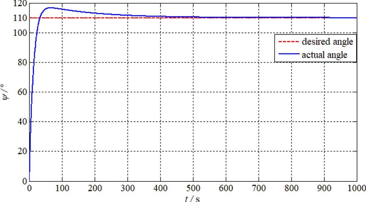
In the absence of disturbance, the initial heading and position are $0^{\circ }$ and $(0,0)$, the desired heading is $110^{\circ }$, initial $u$ is 2 m/s, $V_{{\rm tw}}$ is set as 5 m/s, and the wind blows from the north to the south. According to the Beaufort wind scale, the wind is level 3 the sea state is level 2. The parameters of the traditional SMESC scheme are chosen as $k = 0{\cdot }19$, $\beta = 19$, $\rho = 16$; the parameters of the ESC without steady-state oscillation scheme are $r = 0{\cdot }08$, ${k_1} = 0{\cdot }12$, $\omega = 3$, ${\omega _l} = 0{\cdot }5$, ${\omega _h} = 1{\cdot }5$; the parameters of the SMESC without steady-state oscillation scheme are $k = 0{\cdot }12$, $\beta = 19$, $\rho = 8{\cdot }3$, $r = 0{\cdot }08$, ${k_1} = 1$, $\omega = 3$, ${\omega _l} = 0{\cdot }1$, ${\omega _h} = 1$. The simulations are shown in Figures 7–11.

Figure 7.

The yaw angle $\psi$ curve

Figure 8.

The apparent wind angle $\alpha _{{\rm aw}}$ curve

Figure 9.

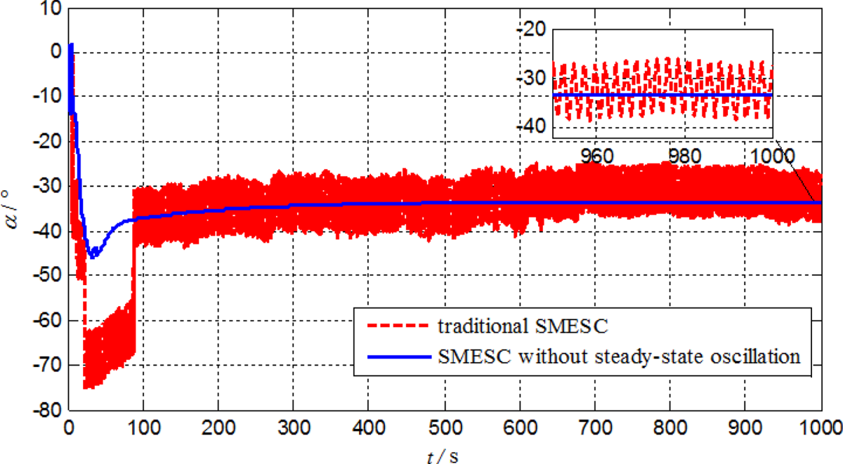
The actual $\alpha$ curve

Figure 10.

The sail angle ${\delta_{\rm s}}$ curve

Figure 11.

The optimisation of $u$ without disturbance

The curve of the unmanned sailboat actual heading is depicted in Figure 7. We can see that the sailboat can be maintained at the desired heading angle. Then, ${\alpha_{\rm aw}}$, $\alpha$ and ${\delta _s}$ are shown in Figures 8–11, respectively, and satisfy ${\delta _s} = {\alpha_{\rm aw}} - \alpha$. It can be seen from the comparison of the two optimisation schemes that the system is gradually stable, and ${\delta _s}$ and $\alpha$ in the SMESC scheme contain large steady-state oscillation. Frequent changes of ${\delta _s}$ will cause instability and shorten the service life of the equipment. However, the scheme we proposed can eliminate the steady-state oscillation.

During the ESC process, $\alpha$ and ${\delta _s}$ are adjusted to the best position to maximise $u$. From Figure 11, we can see the maximum speed is approximately $3{\cdot }832$ m/s as well as the tracking of the optimised speed of three different schemes and the model-based optimal value. The optimised speed of the three different schemes can track the theoretical maximum speed, and the SMESC without steady-state oscillation has the fastest convergence rate. From the locally enlarged image, the optimal speed of the SMESC without steady-state oscillation is superior to the other two schemes, and the steady-state oscillation existing in the SMESC scheme is also eliminated. This validates the effectiveness and better performance of our scheme.

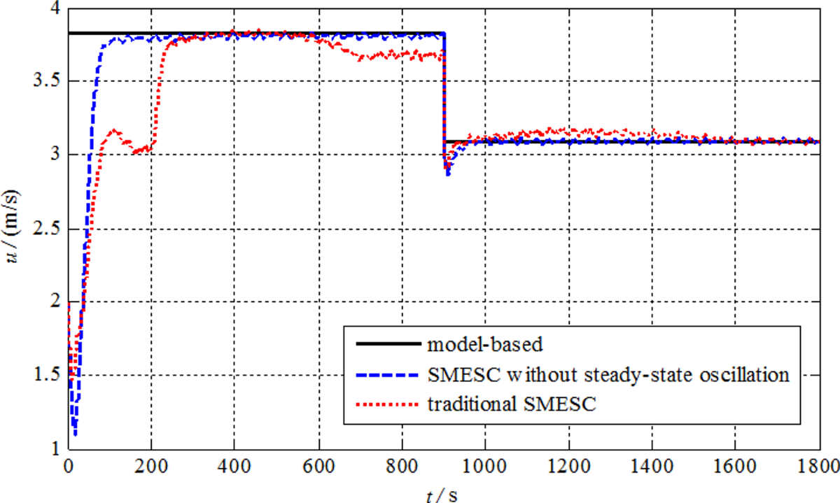
5.2. Simulations with disturbance

Next, simulations are carried out under the condition of disturbance to verify the strong robustness of this improved speed optimisation system, and the wind level and sea state are the same as those in subsection 5.1. The speed extremum point of the system is changed by changing the heading, so as to verify the adaptability of the SMESC without steady-state oscillation scheme for the changing extremum point system. The disturbance parameters are chosen as $T = 2{\cdot }15$ m, $k = 1$, $\mu = {2^ \circ }$, $h = 1$ m, ${\omega _e} = 0{\cdot }3$ Hz, ${\rho _{\rm water}} = 1025$ kg/m$^{3}$. 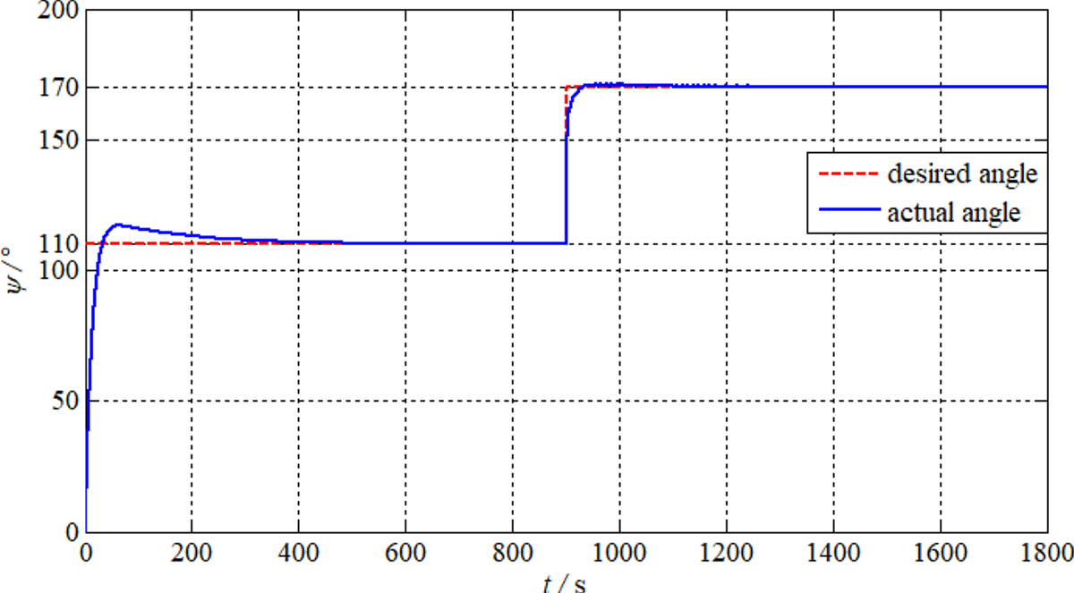We set the desired heading to $11{0^{\circ } }$ before $900$ s, and the desired heading to $170^{\circ }$ after $900$ s. The simulations are shown in Figures 12 and 13.

Figure 12.

The yaw angle $\psi$ curve

Figure 13.

The optimisation of $u$ with disturbance

In Figure 12, the unmanned sailboat can track the desired heading well at two stages. In Figure 13, after the change of the speed extremum point, under the action of the SMESC without steady-state oscillation, the new speed extremum point can still be searched quickly and smoothly. However, the traditional SMESC optimisation scheme has a large deviation from the model-based optimal speed. Therefore, the SMESC without steady-state oscillation still has good adaptability to the changing extremum point system, the convergence rate and stability are better than traditional SMESC, and it is more robust for uncertain variables.

5.3. Speed polar diagram simulations

Finally, to verify the control accuracy of this improved optimisation scheme, the SMESC without steady-state oscillation optimisation speeds are compared with model-based maximum speeds under different headings, as shown in Figure 14.

Figure 14.

The model-based maximum speeds and SMESC without steady-state oscillation results

The speed polar diagram shows the optimal steady-state speeds of unmanned sailboats in different headings, under a given wind condition. Under the sailboat dynamic model, the optimal speeds are obtained by simulation. First, a heading controller adjusts the rudder angle to track the desired heading, then continuously changes ${\delta _{\rm s}}$ to get the model-based maximum speeds. In Figure 14, a comparison between optimal speeds (red marks) based on SMESC without steady-state oscillation and the model-based maximum speeds (blue curve) is given. The results show that most values are matched in both cases. In other words, this novel speed optimisation scheme can ensure high control accuracy, and make the unmanned sailboat sail at the optimal speed state.