1. Introduction
During controlled landing on planetary bodies having a solid surface – e.g. the Moon, Mars, Venus, Titan, Enceladus, Europa as well as asteroids and comets, etc. – jets issued from small rockets are used to position the lander. In the distance between lander and ground, the jets eventually merge into a single jet – a plume – which interacts with the granular soil surface or icy surface, and the jet impingement causes a crater in the surface. Understanding the detailed dynamics and formation of this crater has been one of the important elements in trying to ensure the success of space missions. For example, radar altimetry is used to detect the planetary surface, and to ensure that the lander does not crash onto the surface during descent, the measurement must be able to inform about the actual surface formed during cratering, however, the measurement is biased by the rocket-plume-displaced atmosphere-borne soil/regolith particles; such particles may also obscure cameras positioned on landers. The additional effect of the dispersed particles is that, by acquiring substantial momentum from the plume, they may impinge the lander, possibly damaging it and making it unsafe for Earth return; additionally, such particles may damage the coating of the lander antenna, thereby changing the antenna thermal properties, a fact which can impede transmission of information from the lander to Earth or to an orbiting spacecraft. For example, Jaffe (Reference Jaffe1971) related that when the Apollo 12 landed on the Moon's surface, the jet exhaust dispersed the lunar regolith particles to large distances and speeds in excess of 70 m s $^{-1}$; it is clear that such large speeds and particle flux can cause catastrophic damage to a lander. On planetary bodies with small gravity (e.g. Moon, Titan, Europa, Enceladus), these particles will not settle back onto the surface for a long time, and instead may orbit the planetary body, thus presenting an additional hazard to a lander and to any Earth return mission. Astronauts who landed on the Moon have already reported displaced particles which eventually orbited the Moon, thus obscuring visibility (The Verge 2019). In addition, if the mission is unmanned and involves the search for molecular signs of life (e.g. on Mars or Titan), the probes should not sample the extraterrestrial planetary surface contaminated by the rocket plume. All these considerations clearly indicate that predicting cratering dynamics is of both engineering and scientific interest.
Modelling plume-induced crater formation on a planetary body is a challenging scientific problem as it involves the confluence and interplay of several fluid dynamics phenomena such as turbulence, multiphase interaction, heat transfer, diffusion, inter-particle collisions, etc. The exact dynamics and formation of the crater depend on the characteristics of the jet and of the material which constitutes the planetary surface. The ultimate characteristics of the jet seen by the soil are a combination of the conditions at the exhaust of the rockets and of the interaction of the ultimately formed jet with the existing atmosphere on the planetary body. In some cases, the atmosphere is a very dilute gas (e.g. the Moon, Europa, Enceladus, etc.) so that the jet motion is virtually unimpeded by the atmosphere gas; however, if the atmosphere is very dense (e.g. Venus, Titan, etc.) this interaction will significantly affect the dynamics of the jet impinging the planetary soil. Modelling such dense atmospheres is very challenging, as shown by Toublanc et al. (Reference Toublanc, Parisot, Brillet, Gautier, Raulin and McKay1995).
Several models exist in the literature to investigate jet-induced cratering on a granular bed, and most of these models are based on granular theory. In this theory – borrowing concepts from kinetic theory (KT) of gases – particles are assumed to interact similarly to molecules in a gas and the inter-particle collisions give rise to particle-ensemble macroscopic transport properties such as viscous effects, diffusion, etc. Applying KT to granular media clearly involves a substantial simplification as molecules in gases experience binary collisions, whereas tightly packed particles will experience multiple-particle collisions; in the absence of an established multiple-particle collision theory, the KT complemented by a correction to the dilute regime has led in the context of granular flow to astonishingly qualitatively accurate results. A similarly inspired model for granular flows is the filtered KT model (Parmentier & Simonin Reference Parmentier and Simonin2012; Milioli et al. Reference Milioli, Milioli, Holloway, Agrawal and Sundaresan2013), which has been applied in the past to the study of fluidized beds. However, the closures for the underlying submodels are different for KT and filtered KT models, and the latter is not established for shock-driven flows. Therefore, the classical KT model for granular flows (Gidaspow Reference Gidaspow1994) is utilized in this study.
Since the planetary body atmosphere may be a dilute gas, a gas similar to the Earth lower atmosphere, or a very dense collection of molecules, the best terminology to encompass all these possibilities is to call it a ‘fluid’. If the soil particles are inert, the particle ensemble interacts with the surrounding fluid through momentum and energy exchange, and thus the two phases, i.e. fluid and solid, are intimately coupled. Models for the granular/soil interaction can be divided into two general categories. In the first category are the models addressing complex situations; these models use a combination of fundamentally derived equations and submodels to simulate situations as close as possible to those of practical interest (Liu, Guo & Lin Reference Liu, Guo and Lin2015; Houim & Oran Reference Houim and Oran2016; Balakrishnan & Bellan Reference Balakrishnan and Bellan2018, Reference Balakrishnan and Bellan2019). In the other category are fundamental models considering very simplified situations, with the goal of deriving submodels for the more complex models and/or of examining the range of validity of those complex models (Gidaspow Reference Gidaspow1994; Balakrishnan Reference Balakrishnan2010; Fox Reference Fox2014; Fullmer et al. Reference Fullmer, Liu, Yin and Hrenya2017; Hosseinzadeh-Nik, Subramaniam & Regele Reference Hosseinzadeh-Nik, Subramaniam and Regele2018; Sundaresan, Ozel & Kolehmainen Reference Sundaresan, Ozel and Kolehmainen2018; Shallcross, Fox & Capecelatro Reference Shallcross, Fox and Capecelatro2020). Since all these models involve a multitude of phenomena – interparticle collisions as expressed by the restitution coefficient, interparticle friction due to the particles sliding over each other, fluid drag on the collection of particles as dependent on the volume fraction of particles, etc. – experimental studies (Scott & Ko Reference Scott and Ko1968; Metzger et al. Reference Metzger, Latta, Schuler and Immer2009; Metzger, Smith & Lane Reference Metzger, Smith and Lane2011; Sengupta et al. Reference Sengupta, Kulleck, Van Norman and Mehta2011; Badr, Gauthier & Gondret Reference Badr, Gauthier and Gondret2016) or photographic observations obtained during missions (Colwell et al. Reference Colwell, Batiste, Horányi, Robertson and Sture2007; Mars Science Laboratory) provide valuable information for determining the capability of models to reproduce reality. To the authors’ knowledge, the only model which reproduced photographs taken during the Mars Science Laboratory landing is that of Balakrishnan & Bellan (Reference Balakrishnan and Bellan2018). The craters observed in Balakrishnan & Bellan (Reference Balakrishnan and Bellan2018) were complex geometrical objects with festooned perimeters and radial ridges extending from the perimeter toward the crater nominal centre; physical explanations for the formation of these complex features were provided and the effect of the granular soil characteristics (solid volume fraction, particle diameter, particle material density and collision efficiency) was studied. The same model, enhanced by including frictional pressure effects, was used to explore cratering on Titan (Balakrishnan & Bellan Reference Balakrishnan and Bellan2019). The results were very different from those obtained for Mars: the Titan craters were deeper at same plume Mach number,  $Ma$, and conical in cross-section rather than parabolic as observed for the Mars-like situation. The periphery was not festooned, but a new ephemeral phenomenon of crater-in-crater formation was observed. It seems reasonable to use a successful and versatile model to explore fundamental aspects of interest in the cratering process during controlled landing.
The existence of both parabolic and conical craters is supported by the recent experimental and theoretical study of Badr et al. (Reference Badr, Gauthier and Gondret2016), who showed the significance of the Shields number,  $Sh,$ on subsonic low-speed jet-induced cratering on a granular bed. By definition,
 $Sh\equiv \rho _{f}U_{j} ^{2}/[(\alpha _{s}\rho _{s}-\rho _{f})gd]$ where
 $\rho _{f}$ is the fluid density,
 $U_{j}$ is the mean jet velocity at the outlet,
 $\alpha _{s}$ is the granular-soil density,
 $\rho _{s}$ is the solid material density,
 $g$ is the gravity acceleration and
 $d$ is the particle diameter. Only quasi-steady states, corresponding to dynamic equilibrium, were investigated in Badr et al. (Reference Badr, Gauthier and Gondret2016). The results reported two types of crater morphologies: a shallow parabolic crater (type I) occurring for a weakly deflected jet and deep conical craters (type II) for a strongly deflected jet. The significance of the Shields number was additionally highlighted by Brunier-Coulin, Cuellar & Philippe (Reference Brunier-Coulin, Cuellar and Philippe2017), who have experimentally investigated a water jet impinging on a granular bed under low-speed conditions and constructed an empirical model for quantifying erosion of the bed. For laminar flows, Ouriemi et al. (Reference Ouriemi, Aussillous, Medale, Peysson and Guazzelli2007) explored experimentally the influence of both
 $Sh$ and the Galileo number,
 $Ga\equiv (\rho _{s}-\rho _{f})\rho _{f}gd^{3}/\mu _{f}^{2}$ where
 $\mu _{f}$ is the fluid viscosity, and found a critical
 $Sh$ beyond which the motion of the bed ceases and a steady state is established. Given the low-speed motion considered in both Badr et al. (Reference Badr, Gauthier and Gondret2016) and Ouriemi et al. (Reference Ouriemi, Aussillous, Medale, Peysson and Guazzelli2007), gravity is indeed expected to play and important role and thus
 $Sh$ and
 $Ga,$ as defined, are expected to play an important role. The situation is very different for high-speed flow where gravity forces are minimal compared to drag and the inter-granular frictional stress (Balakrishnan & Bellan Reference Balakrishnan and Bellan2018).
There are many modelling and simulation studies addressing the problem of jet-induced cratering that have shed useful insights on the physics of the problem (Metzger et al. Reference Metzger, Latta, Schuler and Immer2009; Sengupta et al. Reference Sengupta, Kulleck, Van Norman and Mehta2011; Morris et al. Reference Morris, Goldstein, Varghese and Trafton2012, Reference Morris, Goldstein, Varghese and Trafton2015; LaMarche et al. Reference LaMarche, Moran, van Wachem and Curtis2017), albeit they have lower physical fidelity than those of Balakrishnan & Bellan (Reference Balakrishnan and Bellan2018, Reference Balakrishnan and Bellan2019) in that they are either two-dimensional or do not account for all the underlying phenomena of relevance to the problem. A detailed discussion of these past studies can be found in Balakrishnan & Bellan (Reference Balakrishnan and Bellan2018, Reference Balakrishnan and Bellan2019) and is not reproduced here, for brevity. The present investigation addresses the role that the density ratio between plume and planetary atmosphere has on the dynamics of crater formation produced by a supersonic jet; the fluid is assumed to be in the continuum regime. Of particular interest is identifying the behaviour of the flow that only depends on this ratio, and the characteristics of the flow that depend on the fluid density (or pressure). Because a dense atmosphere affords the largest variations in the density ratio while considering realistic (but not necessarily real) jet-fluid densities, the nominal Titan conditions of Balakrishnan & Bellan (Reference Balakrishnan and Bellan2019) are retained. The interest is here in the dynamics of cratering during the early stages of the jet impingement on the granular bed, that is, in the crater evolution when impinged by the jet as opposed to the long-time evolution after the jet shutoff.
The governing equations for the interaction of fluid/granular media are summarized in § 2. The physical interaction between these two media is mathematically expressed through ‘source terms’ in the conservation equations for mass, momentum, chemical-species partial density and energy; the modelling of fluid transport properties is outlined in Appendix A. The configuration and boundary conditions used in the simulations are stated in § 3, including the numerical scheme employed to solve the governing equations. The results and discussion of crucial findings are presented in § 4. Finally, the conclusions obtained from this study are described in § 5. In particular, it is found that another non-dimensional ratio other than  $Sh$ determines the cross-sectional crater shape under supersonic conditions.
2. Governing equations
The conservation equations are developed in an Eulerian framework for both the solid-particle phase and fluid phase. These two-phase flow equations are obtained through several steps. First, a domain averaging is conducted to obtain the volume fraction of each phase using the fundamental methodology of Sirignano (Reference Sirignano1999, Reference Sirignano2005). Second, the fluid equations – consisting of the Navier–Stokes equations for compressible fluids complemented by species and the total energy equation – are filtered to remove the small scales, thus casting these equations in the large eddy simulation (LES) form; the local domain-averaged fluid volume fraction,  $\overline {\alpha _{f}}$, is one of the dependent variables. In this set of equations, the pseudo-turbulent kinetic energy (PTKE) (Moore & Balachandar Reference Moore and Balachandar2019; Shallcross et al. Reference Shallcross, Fox and Capecelatro2020) has been assumed negligible since the particle material density is much larger than that of the ambient fluid and the jet interacts with the particle bed in a stagnation zone where particle-to-fluid velocity differences are small. In regions where the slip velocity between the two phases is small and the particle volume fraction is substantial, large eddy turbulent structures dominate the overall flow field rather than small particle-generated scales; this assumption is supported by the derivation of Igci et al. (Reference Igci, Andrews IV, Sundaresan, Pannala and O'Brien2008). Thus, since the focus is primarily on the crater formation, the PTKE can be considered to have insignificant magnitude compared to that in the large energy-bearing fluid scales that dictate the long-term evolution of the crater. For the granular flow, KT concepts described by kinetic granular theory (see Gidaspow Reference Gidaspow1994; Igci et al. Reference Igci, Andrews IV, Sundaresan, Pannala and O'Brien2008) and relying on particle-ensemble averaging are used to derive the solid-particle phase equations; the local domain-averaged particle-phase volume fraction,
 $\overline {\alpha _{s}}=1-\overline {\alpha _{f}},$ is one of the dependent variables in these equations. The interaction between the two phases – granular medium and fluid – occurs at small scales and is expressed by source terms in both sets of the governing equations. Because the phase interaction occurs at small scales, the subgrid-scale (SGS) model in LES has particular significance. A complete derivation of the governing equations is presented in Balakrishnan & Bellan (Reference Balakrishnan and Bellan2018, Reference Balakrishnan and Bellan2019), and is not duplicated here; only the final form of the equations is presented, for clarity in interpretation of the results.
2.1. Governing equations for the fluid phase
2.1.1. Conservation equations
The domain-averaged LES equations for the fluid phase are (Balakrishnan & Bellan Reference Balakrishnan and Bellan2018, Reference Balakrishnan and Bellan2019)
 \begin{gather} \frac{\partial( \overline{\rho_{f}}) }{\partial t}+\frac {\partial( \overline{\rho_{f}}\tilde{u}_{f,j}) }{\partial x_{j}}=0, \end{gather}
 \begin{gather} \frac{\partial( \overline{\rho_{f}}\tilde{u}_{f,i}) }{\partial t}+\frac{\partial( \overline{\rho_{f}}\tilde{u} _{f,i}\tilde{u}_{f,j}) }{\partial x_{j}}+\frac{\partial( \overline{\alpha_{f}}\hat{p}_{f}) }{\partial x_{i}} =\frac{\partial( \overline{\alpha_{f}}\hat{\sigma}_{f,ij}) }{\partial x_{j}}-\frac{\partial\sigma_{f,ij}^{sgs}}{\partial x_{j}}\nonumber\\ \quad\quad\quad +\,[ \hat{p}_{f}\delta_{ij}-\hat{\sigma}_{f,ij}] \frac{\partial\overline{\alpha_{f}}}{\partial x_{j}}+\overline{\rho_{f}} g_{i}-f_{drag,i}, \end{gather}
 \begin{gather} \hspace{-7pc}\frac{\partial( \overline{\rho_{f}}\tilde{e}_{f,t}) }{\partial t}+\frac{\partial( \overline{\rho_{f}}\tilde{e} _{f,t}\tilde{u}_{f,j}) }{\partial x_{j}}+\frac{\partial( \overline{\alpha_{f}}\tilde{u}_{f,i}[ \hat{p}_{f}\delta _{ij}-\hat{\sigma}_{f,ij}] ) }{\partial x_{j}} \nonumber\\ ={-}\frac{\partial( \overline{\alpha_{f}}\hat{q}_{f,j}) }{\partial x_{j}}+[ \hat{p}_{f}\delta_{ij}-\hat{\sigma} _{f,ij}] \overline{u_{s,i}}\frac{\partial\overline{\alpha_{f}} }{\partial x_{j}}-\frac{\partial\zeta_{f,j}^{sgs}}{\partial x_{j}} -\frac{\partial}{\partial x_{j}}( \overline{\rho_{f}}\tilde{u} _{f,i}\sigma_{f,ij}^{sgs}) \nonumber\\ \hspace{-10.2pc}+\,\overline{\rho_{f}}\tilde{u}_{f,i}g_{i}-f_{drag,i}\overline{u_{s,i} }-q_{conv}, \end{gather}
 \begin{gather} \frac{\partial( \overline{\rho_{f}}\widetilde{Y_{\alpha}}) }{\partial t}+\frac{\partial( \overline{\rho_{f}}\widetilde{Y_{\alpha} }\tilde{u}_{f,j}) }{\partial x_{j}}={-}\frac{\partial( \overline{\alpha_{f}}\hat{J}_{\alpha,j}) }{\partial x_{j}} -\frac{\partial\eta_{\alpha,j}^{sgs}}{\partial x_{j}}. \end{gather}
Here,  $\overline{\rho _{f}}$ is the local domain-averaged filtered fluid density,
 $\tilde{u}_{f,j}$ is the local domain-averaged Favre-averaged fluid velocity in the jth direction,
 $\tilde{e}_{f,t}$ is the local domain-averaged Favre-averaged specific total energy of the fluid (i.e. internal + kinetic energy), and
 $\hat{p}_{f}$ is the local domain-averaged filtered fluid pressure. Also,
 $\overline {u_{s,j}}$ is the local domain-averaged solid-particle phase ensemble-averaged velocity in the
 $j$th direction that arises in the fluid-phase equations due to the assumption that the interface velocity between fluid and solid phases is equal to the solid-particle velocity, this assumption being valid for situations in which the solid-particle material is incompressible (Sirignano Reference Sirignano2005);
 $\hat {\sigma }_{f,ij}$ are the elements of the local domain-averaged filtered shear stress tensor in the fluid that is computed assuming that the fluid is Newtonian,
 \begin{equation} \hat{\sigma}_{f,ij}=2\mu_{f}S_{ij}-\tfrac{2}{3}\mu_{f}\delta_{ij} S_{kk},\quad S_{ij}=\frac{1}{2}\left( \frac{\partial\tilde{u} _{f,i}}{\partial x_{j}} +\frac{\partial\tilde{u}_{f,j}}{\partial x_{i} }\right) . \end{equation}
Here,  $\hat {q}_{f,j}$ are the components of the local domain-averaged filtered heat flux that is here computed using Fourier's law of heat conduction complemented by the enthalpy transported by the species (see (2.6)). The local domain-averaged Favre-averaged mass fraction of the species is denoted by
 $\tilde {Y}_{\alpha }$, where subscript
 $\alpha$ labels the species, and
 $\hat {J}_{\alpha ,j}$ are the components of the local domain-averaged filtered
 $\alpha$-species diffusion flux. The fluxes are computed from
 \begin{align} \hat{\boldsymbol{q}}_{f} &={-}\lambda_{f}\boldsymbol{\nabla}\hat{T}_{f}+\sum _{\alpha=1}^{N-1}\hat{\boldsymbol{J}}_{\alpha}\left[ \left( \frac {\hat{h}_{\alpha}}{m_{\alpha}}-\frac{\hat{h}_{N}}{m_{N}}\right) -R_{u}\hat{T}_{f}\left( \frac{\bar{\alpha}_{T,\alpha}^{b}}{m_{\alpha} }-\frac{\bar{\alpha}_{T,N}^{b}}{m_{N}}\right) \right] , \end{align}
 \begin{align}\hat{\boldsymbol{J}}_{\alpha,f} &={-}\overline{\rho_{f}}\left[ \tilde{Y}_{\alpha}(D_{T,\alpha}) \frac{\boldsymbol{\nabla}\hat{T}_{f}} {\hat{T}_{f}}+\tilde{Y}_{\alpha}(D_{p,\alpha}) \frac{\boldsymbol{\nabla}\hat{p}_{f}}{\hat{p}_{f}}+\sum_{\beta=1}^{N-1}\left( D_{\alpha\beta}^{\prime}\frac{m_{\alpha}}{m_{\beta}}\right) \boldsymbol{\nabla} \tilde{Y}_{\beta}\right] , \end{align}
where  $\hat {T}_{f}$ is the local domain-averaged filtered fluid temperature, and
 $D_{T,\alpha },D_{p,\alpha }$ and
 $D_{\alpha \beta }^{\prime }$ are diffusion coefficients
 \begin{gather} D_{T,\alpha}={-}\sum_{\beta=1}^{N}\bar{\alpha}_{T,\beta}^{b}\mathbb{D} _{\beta\alpha},\quad D_{p,\alpha}=\frac{\hat{p}_{f}}{R_{u} \hat{T}_{f}}\sum_{\beta=1}^{N}v_{\beta}\mathbb{D}_{\beta\alpha},\quad D_{\alpha\gamma}=\sum_{\beta=1}^{N}\mathbb{D}_{\alpha\beta} \alpha_{D\beta\gamma}, \end{gather}
 \begin{gather}\bar{\alpha}_{T,\alpha}^{b}=\sum_{\beta=1}^{N}\tilde{X}_{\beta} \alpha_{T,\beta\alpha}^{b},\quad D_{\alpha\beta}^{\prime} =D_{\alpha\beta}-\left( 1-\frac{m_{\beta}}{m_{N}}\right) \left( \sum_{\gamma=1}^{N-1}D_{\alpha\gamma}\tilde{X}_{\gamma}\right). \end{gather}
The  $\hat {\boldsymbol {J}}_{\alpha }$ and
 $\hat {\boldsymbol {q}}_{f}$ expressions are based on the full matrices of mass-diffusion coefficients and thermal-diffusion factors derived in Harstad & Bellan (Reference Harstad and Bellan2004a). In order to ensure global mass conservation, a set of independent (
 $N-1)$ species equations is considered rather than the set of
 $N$ dependent species; in these (
 $N-1)$ equations, the original molar-fraction fluxes and the heat flux are rewritten to account for only (
 $N-1)$ gradients. Here,
 $\tilde {X}_{\alpha }=\tilde {Y}_{\alpha }m/m_{\alpha }$ represents the local domain-averaged filtered molar fraction;
 $m_{\alpha }$ is the species molar mass;
 $m$ is the mixture molar mass,
 $m=\sum_{\gamma =1}^{N}m_{\gamma }\tilde{X}_{\gamma }, v_{\alpha }=(\partial v/\partial X_{\alpha })_{T,p,X_{\beta }(\beta \!\neq \alpha )}$ is the partial molar volume, where the molar volume is
 $v=m/\rho$;
 $h_{\alpha }=(\partial h/\partial \tilde {X}_{\alpha })_{\hat {T}_{f},\hat {p} _{f},\tilde {X}_{\beta }(\beta \!\neq \alpha )}$ is the partial molar enthalpy, where the molar enthalpy is
 $\hat {h}=G-\hat {T}_{f}(\partial G/\partial \hat {T}_{f})_{\hat {p},\tilde {X}}$ with
 $G$ being the Gibbs energy
 $; R_{u}$ is the universal gas constant;
 $D_{\alpha \gamma }$ are the pairwise mass-diffusion coefficients;
 $\alpha _{T,\alpha \beta }^{b}$ are the binary thermal-diffusion factors; and
 $\lambda _{f}$ is the thermal conductivity of the fluid.
The mass-diffusion factors,  $\alpha _{D\alpha \beta },$ are calculated from thermodynamics as
 \begin{gather} \alpha_{D\alpha\beta} \equiv\frac{1}{R_{u}\hat{T}} \tilde{X}_{\alpha}\frac{\partial\mu_{\alpha}}{\partial\tilde{X}_{\beta} }=(\delta_{\alpha\beta}-\delta_{\alpha N})+\tilde{X}_{\alpha} (R_{\alpha\beta}-R_{\alpha N}),\quad 1\leqslant\alpha\leqslant N,\text{ }1\leqslant\beta\leqslant N-1, \end{gather}
 \begin{gather}R_{\alpha\beta} \equiv\frac{\partial\ln\gamma_{\alpha}}{\partial X_{\beta }},\quad 1\leqslant\alpha\leqslant N,\ 1\leqslant \beta\leqslant N, \end{gather}
where  $\mu _{\alpha }$ is the chemical potential of species
 $\alpha$ written in terms of
 $N-1$ species;
 $\gamma _{\alpha }\equiv \varphi _{\alpha }/\varphi _{\alpha }^{\circ} $ where
 $\varphi$ is the fugacity coefficient written in terms of
 $N$ species and the superscript
 $o$ denotes the pure (
 $\tilde {X}_{\alpha }=1)$ limit; for a perfect gas, the fugacity is identified with the pressure and thus the fugacity coefficients are equal to unity; thus, for perfect gases the second term in (2.10) is null. Matrix elements
 $\mathbb {D}_{\beta \gamma }$ are the solution of the mixing rules equations (Harstad & Bellan Reference Harstad and Bellan2004a)
 \begin{equation} \sum_{\beta=1}^{N}\left[ \delta_{\alpha\beta}-( 1-\delta_{\alpha\beta }) \tilde{X}_{\beta}\frac{\mathcal{\bar{D}}_{\alpha}} {\mathcal{D}_{\alpha\beta}^{b}}\right] \frac{\mathbb{D}_{\beta\gamma} }{\tilde{X}_{\beta}}=\mathcal{\bar{D}}_{\alpha}\frac{(\delta_{\alpha\gamma}-\tilde{Y}_{\alpha})}{\tilde{X}_{\alpha}}, \end{equation}
where
 \begin{equation} \mathcal{\bar{D}}_{\alpha}=1\left/\sum_{\substack{\beta=1\\\beta\!\!\neq\alpha }}^{N}\left( \frac{\tilde{X}_{\beta}}{\mathcal{D}_{\alpha\beta}^{b} }\right) \right. . \end{equation}
Solutions for  $\mathbb {D}_{\beta \gamma }$ may be obtained by an approximate inversion (Ern & Giovangigli Reference Ern and Giovangigli1998) as follows:
 \begin{gather} \mathbb{D}_{\beta\gamma} \simeq\tilde{X}_{\beta}\mathbb{D} _{\beta\gamma}^{(1) }, \end{gather}
 \begin{gather}\quad\quad \mathbb{D}_{\alpha\beta}^{(1) } =\frac{( 1+\tilde{Y}_{\alpha}) }{\tilde{X}_{\alpha}}\mathcal{D}_{\alpha }^{{\ast}}\delta_{\alpha\beta}+( 1-\delta_{\alpha\beta}) \frac{\mathcal{D}_{\alpha}^{{\ast}}\mathcal{D}_{\beta}^{{\ast}}}{\mathcal{D} _{\alpha\beta}^{b}}-( \sigma_{\alpha}\mathcal{D}_{\alpha}^{{\ast}} +\sigma_{\beta}\mathcal{D}_{\beta}^{{\ast}}) +\sum_{\gamma=1}^{N}( \tilde{Y}_{\gamma}\sigma_{\gamma}\mathcal{D}_{\gamma}^{{\ast}}) , \end{gather}
 \begin{gather}\mathcal{D}_{\alpha}^{{\ast}} =( 1-\tilde{Y}_{\alpha}) \mathcal{\bar{D}}_{\alpha}, \end{gather}
 \begin{gather}\sigma_{\alpha} =\frac{m_{\alpha}}{m}( 1+\tilde{Y}_{\alpha }) +\sum_{\substack{\beta=1\\\beta\!\neq\alpha}}^{N}\tilde{Y}_{\beta }\frac{\mathcal{D}_{\beta}^{{\ast}}}{\mathcal{D}_{\alpha\beta}^{b}}, \end{gather}
where  ${\mathcal {D}_{\alpha \beta }^{b}}$ is the full approximation binary-diffusion matrix. This method leads to a singularity when the mixture is composed of only one species. In that case, (2.13) is no longer used and the diffusion coefficients are evaluated using the binary-diffusion matrix, by setting
 $\mathcal {D}_{\alpha }^{\ast }= \mathcal {D}_{\alpha N}^{b}$, where
 $N$ represents the index associated with the solvent. This method was tested against an exact Gauss inversion (not shown) and it gave the same results, with an additional gain in computational time. Defining
 $\mathcal {D}_{\alpha \beta }$ as the first approximation of the binary-diffusion matrix and realizing that the deviation of the ratio
 $\mathcal {D}_{\alpha \beta }^{b}/\mathcal {D}_{\alpha \beta }$ from unity is comparable to uncertainties in the binary-diffusion coefficient values (Harstad & Bellan Reference Harstad and Bellan2004a), we assume
 $\mathcal {D}_{\alpha \beta }^{b}=\mathcal {D} _{\alpha \beta }$. The computation of
 ${\mathcal {D}_{\alpha \beta }^{{}}}$ and
 $\alpha _{T,\alpha \beta }^{b}$ is described in Appendix A along with the other transport properties.
The quantities  $\sigma _{f,ij}^{sgs}$,
 $\zeta _{f,j}^{sgs}$ and
 $\eta _{\alpha ,j}^{sgs}$
 \begin{equation} \sigma_{f,ij}^{sgs}=\overline{\rho_{f}u_{f,i}u_{f,j}}-\overline{\rho_{f} }\tilde{u}_{f,i}\tilde{u}_{f,j},\quad \zeta_{f,j} ^{sgs}=\overline{\rho_{f}h_{f}u_{f,j}}-\overline{\rho_{f}}\tilde{h} _{f}\tilde{u}_{f,j},\quad \eta_{\alpha,j}^{sgs}=\overline{\rho _{f}Y_{\alpha}u_{f,j}}-\overline{\rho_{f}}\tilde{Y}_{\alpha} \tilde{u}_{f,j}, \end{equation}
are the local SGS stress tensor, the local SGS enthalpy flux and the local SGS  $\alpha$-species. These terms represent in the conservation equations the effects that are filtered away;
 $\sigma _{f,ij}^{sgs}$,
 $\zeta _{f,j}^{sgs}$ and
 $\eta _{\alpha ,j}^{sgs}$ must be modelled as functions of the known flow field solution represented by
 $(\overline {\rho _{f}},\tilde {u}_{f,i},\tilde {e} _{f,t},\tilde {Y}_{\alpha },\hat {p}_{f})$. These SGS terms are modelled using the Smagorinsky (Reference Smagorinsky1963) formulation, which for the stress terms is combined with the Yoshizawa (Reference Yoshizawa1986) model in order to capture the behaviour of the trace term; more details are provided in Balakrishnan & Bellan (Reference Balakrishnan and Bellan2018), including the value of the proportionality constants employed in the model.
2.1.2. Equation of state
The equation of state (EOS) provides the necessary relationship to close the system of governing equations. In contrast to the conservation equations, the EOS is a relationship which holds at any scale, and thus the local domain-averaged filtered dependent variables are used. The atmospheric density for the present conditions is approximately five times that on Earth (Balakrishnan & Bellan Reference Balakrishnan and Bellan2019); thus the terminology of ‘gas’ is inappropriate, and instead it is called a ‘fluid’. This fluid still behaves as a calorically perfect gas and therefore  $\hat {h}_{\alpha } = ({C_{p,\alpha } }/{m_{\alpha }})\hat {T}_{f}$, where
 $C_{p,\alpha }$ is the specific heat at constant pressure of the
 $\alpha$ species (units are J (kmole K)
 $^{-1}$). It follows that the specific heat at constant volume for each species is
 $C_{v,\alpha }=C_{p,\alpha }-R_{u}$ where
 $R_{u}$ is the universal gas constant, and the specific heat ratio of the mixture is evaluated by molar averaging as
 \begin{equation} \gamma_{mix}=\frac{\displaystyle\sum_{\alpha=1}^{N}\frac{C_{p,\alpha}}{m_{\alpha} }\tilde{Y}_{\alpha}}{\displaystyle\sum_{\alpha=1}^{N}\frac{C_{v,\alpha}}{m_{\alpha} }\tilde{Y}_{\alpha}}. \end{equation}
For simplicity, the speed of sound,  $a_{f},$ for the mixture is calculated as if it were a perfect gas, leading to
 \begin{equation} a_{f}=\sqrt{\gamma_{mix}\frac{R_{u}}{m}\hat{T}_{f}}. \end{equation}
2.2. Governing equations for the solid phase
As already stated, the solid phase is modelled using the KT-modified approach of Gidaspow (Reference Gidaspow1994), which adapts the KT of gases outlined in Chapman & Cowling (Reference Chapman and Cowling1970) to particles. Here, paralleling the classical KT, a probability density function is employed to derive consistent expressions for the conservation of mass, momentum and energy of the solid-particle phase. The present situation addresses large values of  $\overline {\alpha _{s}}$ representative of a granular bed of solid particles and thus the appropriate physics is that of the dense regime. For this reason, the Boltzmann equation (Gidaspow Reference Gidaspow1994) is used in conjunction with the Jenkins–Savage transport equation (Jenkins & Savage Reference Jenkins and Savage1983) for the dense regime to derive the governing equations for the solid phase. The complete derivation is presented in Balakrishnan & Bellan (Reference Balakrishnan and Bellan2018, Reference Balakrishnan and Bellan2019), and only the final result is displayed here, for brevity. These equations are
 \begin{gather} \frac{\partial}{\partial t}( \overline{\alpha_{s}}\rho_{s}) +\frac{\partial}{\partial\boldsymbol{x}}( \overline{\alpha_{s}}\rho _{s}\bar{\boldsymbol{u}}_{s}) =0, \end{gather}
 \begin{gather}\quad\frac{\partial}{\partial t}( \overline{\alpha_{s}}\rho_{s} \bar{\boldsymbol{u}}_{s}) +\frac{\partial}{\partial\boldsymbol{x}}( \overline{\alpha_{s}}\rho_{s}\bar{\boldsymbol{u}}_{s}\overline{\boldsymbol{u} }_{s}) +\frac{\partial}{\partial\boldsymbol{x}}( \boldsymbol{\mathsf{P}} _{k}+\boldsymbol{\mathsf{P}}_{c}) +\frac{\partial}{\partial\boldsymbol{x}}( p_{fric}) =\overline{\alpha_{s}}\rho_{s}\boldsymbol{g}+\boldsymbol{f} _{drag}-\overline{\alpha_{s}}\frac{\partial\hat{p}_{f}}{\partial \boldsymbol{x}}, \end{gather}
 \begin{gather} \frac{3}{2}\left[\frac{\partial }{\partial t}\left( \overline{\alpha _{s}}\rho _{s}\varTheta \right) +\frac{\partial }{\partial {\boldsymbol{x}}}(\overline{\alpha _{s}}\rho _{s}\overline{{\boldsymbol{u}}}_{s}\varTheta )\right] ={-}( \boldsymbol{\mathsf{P}}_{k}+\boldsymbol{\mathsf{P}}_{c})\ \textbf{:}\ \frac{\partial \bar{\boldsymbol{u}}_{s}}{\partial\boldsymbol{x}}-\frac{\partial}{\partial\boldsymbol{x}} (\boldsymbol{q}_{k}+\boldsymbol{q}_{c})\nonumber\\ \hspace{11.5pc} +N_{c}+\overline{\alpha_{s}}\rho_{s}( \overline{\boldsymbol{F}_{s} \boldsymbol{\cdot}\boldsymbol{c}}-\boldsymbol{F}\boldsymbol{\cdot}\bar{\boldsymbol{u}}_{s}), \end{gather}
 \begin{gather} \frac{\partial}{\partial t}( \overline{\alpha_{s}}\rho_{s} \overline{e_{s}}) +\frac{\partial}{\partial\boldsymbol{x}}( \overline{\alpha_{s}}\rho_{s}\bar{\boldsymbol{u}}_{s}\overline{e_{s}}) =q_{conv}, \end{gather}
where  $\rho _{s}$ is the particle material density and is a constant,
 $\bar {\boldsymbol {u}}_{s}$ is the ensemble-averaged solid-phase velocity,
 $\boldsymbol{\mathsf{P}}_{c}$ is the collisional pressure tensor stemming from particle collisions,
 $\boldsymbol{\mathsf{P}}_{k}$ is the kinetic pressure tensor due to the motion of the particles,
 $p_{fric}$ is the frictional pressure that arises from inter-particle contact prevalent at high solid volume fractions (
 $\overline {\alpha _{s}}>$ 0.5 Johnson & Jackson Reference Johnson and Jackson1987),
 $\varTheta$ is the granular temperature,
 $\boldsymbol {q}_{k}$ is the heat flux due to kinetic effects and
 $\boldsymbol {q}_{c}$ is its collisional counterpart. Finally,
 $\overline {e_{s}}$ is the ensemble-averaged internal energy of the solid phase due to thermal effects.
The forces acting on the particles are gravity ( $\boldsymbol {g}$), the inter-phase drag (
 $\boldsymbol {f}_{drag}$), the fluid pressure gradient
 $\boldsymbol {\nabla }\hat {p} _{f}$ and the inter-granular stress
 $p_{fric}$. Forces in the particle phase not due to the fluid can be either due to collisions, or due to friction that arises from continuous contact of contiguous particles. KT accounts for collisional effects between particles only (embedded in
 $\boldsymbol{\mathsf{P}}_{c}$ and
 $\boldsymbol {q}_{c})$, and thus alternate closures are necessary for frictional effects in the particle phase, particularly at large
 $\overline {\alpha _{s}}$ values. Frictional viscosity is here neglected in the particle phase (Huilin et al. Reference Huilin, Yurong, Wentie, Ding, Gidaspow and Bouillard2004), but the inviscid contribution of friction, i.e.
 $p_{fric},$ is taken into account (see below). Thus, friction manifests here in normal compression/rarefaction (through
 $p_{fric}$), but not in shear effects. Since frictional viscosity is material-dependent through the angle of internal friction (Huilin et al. Reference Huilin, Yurong, Wentie, Ding, Gidaspow and Bouillard2004), that may not be always known, neglecting frictional viscosity effects has here the advantage of making the present findings material independent. The
 $p_{fric}$ term was not specifically used in the original KT-based model of Gidaspow (Reference Gidaspow1994) as it is not a collisional effect, but is rather due to continuous contact among particles, which is not accounted for in KT. For dense granular flows,
 $p_{fric}$ allows a resistance to close packing. For example, close to the maximum packing limit, the solid particles touch each other and this yields a stress which is in effect a resistance to the theoretical maximum packing compaction defined by the solid fraction
 $\alpha _{s,max}$. The
 $p_{fric}$ term in (2.22) models semi-empirically this effect, thus ensuring that
 $\overline {\alpha _{s} }<\alpha _{s,max}$; the mathematical expression used for
 $p_{fric}$ in this study is that of Johnson & Jackson (Reference Johnson and Jackson1987) and Houim & Oran (Reference Houim and Oran2016)
 \begin{equation} p_{fric}=\left\{ \begin{array}{@{}ll} 0, & \text{if }\overline{\alpha_{s}}<\alpha_{s,crit};\\ p_{fric}^{\circ}\overline{\alpha_{s}}\dfrac{( \overline{\alpha_{s}} -\alpha_{s,crit})^{2}}{( \alpha_{s,max}-\overline{\alpha_{s} })^{5}}, & \text{otherwise.} \end{array} \right. \end{equation}
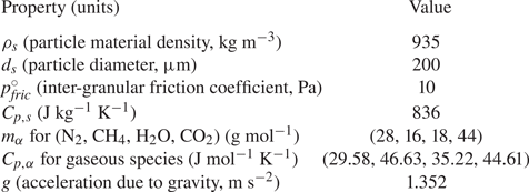
In (2.25),  $\alpha _{s,crit} = 0.5$ is the critical solid volume fraction (Johnson & Jackson Reference Johnson and Jackson1987; Houim & Oran Reference Houim and Oran2016) at which the inter-granular stress comes into play,
 $\alpha _{s,max} = 0.7405$ is the maximum packing limit and
 $p_{fric}^{\circ} $ is a constant having a value empirically fixed; the effect of the
 $p_{fric}^{\circ} $ value was investigated by Balakrishnan & Bellan (Reference Balakrishnan and Bellan2019) and it was found that its magnitude influences the peak compaction
 $\overline {\alpha _{s}}$ value at the interior crater vertically oriented walls and on the crater base. Other forms of the inter-granular stress also exist in the literature (Nigmatulin Reference Nigmatulin1979, Reference Nigmatulin1991; Houim & Oran Reference Houim and Oran2016), but the present one is adopted because of its mathematical simplicity. In the plastic limit one may need to revisit this expression for
 $p_{fric}$ as the material yields to the applied load, which may necessitate the use of alternative formulations (Sundaresan Reference Sundaresan2020). Such plastic limit deformations in the solid particles are not included in the present formulation because the jet strikes the granular bed in a stagnation zone where the slip velocity between the two phases is relatively small, and thus the load on the particles is less than that needed for plastic limit deformations. Thus, the particles are assumed to be in the elastic limit of the yield stress curve where the above
 $p_{fric}$ expression is valid.
The term  $\boldsymbol {f}_{drag}$ is the drag force which arises due to inter-phase momentum transfer between the two phases, and
 $q_{conv}$ denotes the convective heat transfer between the two phases that in particular changes each particle internal energy;
 $\boldsymbol {f}_{drag}$ depends on the slip velocity between the two phases and
 $q_{conv}$ depends on the temperature difference. These terms are described in Balakrishnan & Bellan (Reference Balakrishnan and Bellan2018) and are not presented here, for brevity.
In (2.23), the first term on the right-hand side constitutes the production of granular fluctuations due to shear, the second term represents the heat flux due to kinetic and collisional effects, the third term expresses the dissipation of granular energy due to inelastic collisions, and the last term represents the production and dissipation of granular energy due to interaction with the fluid. Finally, the thermal energy of the solid phase is evaluated as
 \begin{equation} \overline{e_{s}}=\int_{T^{^{\prime}}=0}^{T^{^{\prime}}=\overline{T_{s}} }C_{p,s} \left( T^{^{\prime}}\right) \, \textrm{d} T^{^{\prime}} ,\end{equation}
in which  $\overline {T_{s}}$ is the average temperature of the particle material and
 $C_{p,s}$ is the specific heat capacity of the solid phase. In this study, we assume that
 $C_{p,s}$ is a constant, and thus
 $\overline {e_{s} }=C_{p,s}\overline {T_{s}}$. In summary, the solid phase is governed by (2.21)–(2.24). The source term
 $N_{c},$ in the granular temperature equation (see (2.23)) is the result of inelastic collisions, and is evaluated from the collisional integral using the methods of KT;
 $\boldsymbol {F}_{s} \boldsymbol {\cdot }\boldsymbol {c}-\boldsymbol {F}\boldsymbol {\cdot }\bar {u}_{s}$ is a source term in the granular temperature equation stemming from viscous drag between the fluid and the solid particles.
The model for  $\boldsymbol{\mathsf{P}}_{k}$ is obtained as (Gidaspow Reference Gidaspow1994):
 \begin{equation} \boldsymbol{\mathsf{P}}_{k}=\overline{\alpha_{s}}\rho_{s}\varTheta\boldsymbol{\mathsf{I}}, \end{equation}
where  $\boldsymbol{\mathsf{I}}$ is the identity matrix. Tensor
 $\boldsymbol{\mathsf{P}}_{c}$ is comprised of two components which are evaluated from the collisional integral using the formulation of Jenkins & Savage (Reference Jenkins and Savage1983) (for details, see pp. 284–290 of Gidaspow (Reference Gidaspow1994));
 $\boldsymbol{\mathsf{P}}_{c}=\boldsymbol{\mathsf{P}}_{c,1}+\boldsymbol{\mathsf{P}}_{c,2}$, where
 \begin{equation} \left. \begin{gathered} \boldsymbol{\mathsf{P}}_{c,1} =2(1+e)g_{0}\rho_{s}\overline{\alpha_{s}}^{2} \varTheta\boldsymbol{\mathsf{I}},\\ \boldsymbol{\mathsf{P}}_{c,2} ={-}2\overline{\alpha_{s}}\mu_{sc}\left( \dfrac {\partial\bar{\boldsymbol{u}}_{s}}{\partial\boldsymbol{x}}\right) _{symm.} -\overline{\alpha_{s}}\xi_{s}\dfrac{\partial\bar{u}_{s,i}}{\partial x_{i} }\boldsymbol{\mathsf{I}}, \end{gathered}\right\} \end{equation}
where the subscript  $symm$ refers to the symmetric part of the velocity gradient tensor,
 $e$ is the coefficient of restitution,
 $g_{0}$ is the radial distribution function which is a measure of the probability of finding a particle at a specified distance from a given particle and is interpreted as a non-dimensional distance between the centres of two spheres during a collision event, and
 $\mu _{sc}$ and
 $\xi _{s}$ are the dynamic and bulk viscosity coefficients, respectively, associated with the collisional processes in the particle flow (Gidaspow Reference Gidaspow1994). These viscosity coefficients are computed by comparing the KT derivations of Chapman & Cowling (Reference Chapman and Cowling1970) and the granular flow results of Ding & Gidaspow (Reference Ding and Gidaspow1990) (see pp. 288–289 of Gidaspow (Reference Gidaspow1994) for more details)
 \begin{equation} \left. \begin{gathered} \mu_{sc} =\dfrac{4}{5}\overline{\alpha_{s}}\rho_{s}d_{s}g_{0} (1+e)\sqrt{\dfrac{\varTheta}{\rm \pi},}\\ \xi_{s} =\dfrac{4}{3}\overline{\alpha_{s}}\rho_{s}d_{s}g_{0}(1+e)\sqrt {\dfrac{\varTheta}{\rm \pi}}, \end{gathered}\right\} \end{equation}
where  $d_{s}$ is the particle diameter. Expressions for
 $\boldsymbol {f} _{drag},g_{0}$ and
 $\boldsymbol {F}_{s}\boldsymbol {\cdot }\boldsymbol {c}-\boldsymbol {F}\boldsymbol {\cdot } \bar {u}_{s}$ are provided in Gidaspow (Reference Gidaspow1994) and Balakrishnan & Bellan (Reference Balakrishnan and Bellan2018) and are omitted here, for brevity.
3. Configuration, numerical aspects and boundary and initial conditions
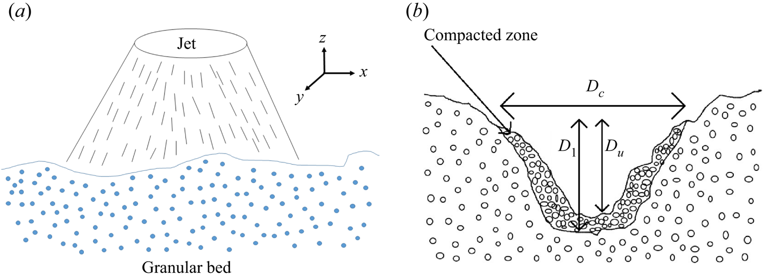
For all simulations in this study, the configuration is that of a three-dimensional domain of size  $4.5\ \textrm {m} \times 4.5\ \textrm {m} \times 9.6\ \textrm {m}$, as shown in figure 1(a) with the coordinates defined as
 $-2.25\ \textrm {m} \leq x\equiv x_{1}\leq 2.25\ \textrm {m}$,
 $-2.25\ \textrm {m} \leq y\equiv x_{2}\leq 2.25\ \textrm {m}$ and
 $-3.6\ \textrm {m} \leq z\equiv x_{3}\leq 6\ \textrm {m}$, where the plane
 $z=0$ m represents the undisturbed granular bed surface. The properties of the granular soil are listed in table 1. The
 $\rho _{s} = O(10^{3}$ kg m
 $^{-3}$) value is consistent with soil particle material density on Earth, or regolith on the Moon, Mars and Titan.
Schematic of (a) the supersonic jet interacting with the granular particle bed; (b) the crater formed in the granular bed.

Values of properties and coefficients used in this study.

The diameter of the jet nozzle exit is  $D_{j} = 0.2$ m and the jet is positioned at the centre of the
 $z=6$ m plane, facing downward. Supersonic outflow boundary conditions (Hirsch Reference Hirsch2007) are used at
 $x=\pm 2.25$ m,
 $y=\pm 2.25$ m and
 $z=-3.6$ m, while at the upper domain boundary free-slip wall conditions are implemented except for the circular nozzle orifice at the centre of the
 $z=6$ m plane where a supersonic inflow boundary condition is employed.
Four species ( $N = 4$) are considered for the simulations: N
 $_{2}$, CH
 $_{4}$, H
 $_{2}$O, CO
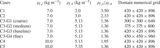
 $_{2}$. The simulations are listed in table 2. The conditions of the simulations are such that it is possible to study the effect of the specified jet density,
 $\rho _{f,j},$ at constant
 $\rho _{f,a}$ by comparing cases C3 and C4, the impact of the ambient atmospheric density,
 $\rho _{f,a},$ at constant
 $\rho _{f,j}$ by examining cases C1, C2 and C3, and to determine those characteristics which are only function of
 $\rho _{f,j} /\rho _{f,a},$ independent of the values of
 $\rho _{f,j}$ and
 $\rho _{f,a},$ by analysing cases C3 and C5. To show that the results are statistically independent of the numerical grid used in the computation, a systematic typical approach to grid convergence – adapted to the present investigation – is also undertaken by considering for case C3 four different grid sizes denoted as: coarse (G1), medium (G2), baseline (G3) and fine (G4). As it is typical for LES, a grid convergence study is performed. Similar to LES of jets, the inquiry is in whether statistical quantities of interest (e.g. here crater length scales) are predicted to have the same value when the grid is refined. In this regard, grid G1 has
 $57.6\times 10^{6}$ nodes, grid G2 has
 $112.5\times 10^{6}$ nodes, grid G3 has
 $158.05\times 10^{6}$ nodes and grid G4
 $194.4\times 10^{6}$ nodes. Therefore, the ratio of the number of nodes between the finest (G4) and the coarsest (G1) simulations is 3.375, and between G4 and G3 is 1.23. Other conditions of the simulations are listed in the caption of table 2. All parameters relevant to the simulations are summarized in table 1.
List of simulations. In all cases the jet temperature is 300 K, and the ambient temperature is 94 K, corresponding to the conditions on Titan. The jet exit plane Mach number is 1.5. The jet composition is  $Y_{{\textrm {N}_2}} = 0.33$,
 $Y_{{\textrm {H}_2}\textrm {O}} = 0.34$,
 $Y_{{\textrm {CO}_2}} = 0.33$ and the ambient composition is
 $Y_{{\textrm {N}_2}} = 0.99$ and
 $Y_{{\textrm {CH}_4}} = 0.01$, corresponding to that of Titan.

The axial velocity of the jet is initialized as a hyperbolic tangent profile and is seeded with perturbations similar to Freund (Reference Freund2001); see Balakrishnan & Bellan (Reference Balakrishnan and Bellan2018, Reference Balakrishnan and Bellan2019) for more details on the perturbations. The  $z\in \lbrack -3.6,0]$ m part of the domain consists of the granular bed of solid particles of height 3.6 m (see figure 1a). To simulate a realistic terrain, a perturbation is added to the interface between the atmosphere and the granular bed in order to mimic an uneven granular surface. This perturbation is implemented in the (
 $x$,
 $y$) plane on the surface at
 $z = z_{surface}=0$ as a multi-mode perturbation with wavelength
 $L = 2$ m; the mathematical form is presented in detail elsewhere (Balakrishnan & Bellan Reference Balakrishnan and Bellan2018).
The Reynolds number based on the mean flow is calculated as  $Re= {\rho _{f,j}U_{f,j}D_{j}}/{\mu _{f}}$, where
 $\rho _{f,j}$ and
 $U_{f,j}$ are the fluid velocity and vertical velocity at the jet exhaust plane,
 $D_{j}$ is the jet diameter, and
 $\mu _{f}$ is the mean fluid viscosity. Using values of
 $\rho _{f,j} = 7$ kg m
 $^{-3}$,
 $U_{f,j} = 530$ m s
 $^{-1}$,
 $D_{j} = 0.2$ m,
 $\mu _{f} = 2\times 10^{-5}$ Pa s, one computes
 $Re = 3.7 \times 10^{7}$, which is a value in the turbulent regime, clearly justifying the use of the LES approach. With increasing
 $\rho _{f,j}$ at same
 $\rho _{f,j} /\rho _{f,a}$ value, the
 $Re$ value increases.
The computations are initialized with  $\overline {\alpha _{s}} = 0.45$ in the particle bed and zero elsewhere. This initialization is meant to be sufficiently far from the close packing limit so that there is sufficient time for the crater and flow to show development and evolution features. The value of 0.45 was thus arbitrarily chosen, as this study is generic. For a granular medium which is not close to maximum packing, physical consistency implies that there should be a finite value
 $\varTheta$. Thus,
 $\varTheta = 10$ m
 $^{2}$ s
 $^{-2}$ is used as an initial value; for more information on the choice of this value, see Liu et al. (Reference Liu, Guo and Lin2015). Since (2.23) has dissipative terms,
 $\varTheta$ quickly decays to negligible values compared to 10 m
 $^{2}$ s
 $^{-2}$, that is, the unsteadiness and dissipation adjust this value to that consistent with the physics of the problem. Essentially, as time increases, the granular flow loses memory of the initial
 $\varTheta$ value, similarly to turbulent flows losing memory of the initial condition.
The governing equations are solved using a finite difference scheme. To obtain the inter-cell fluxes, the fifth-order weighted essentially non-oscillatory (WENO) scheme is used for spatial interpolation (Liu, Osher & Chan Reference Liu, Osher and Chan1994; Jiang & Shu Reference Jiang and Shu1996), including the Rusanov flux solver (Rusanov Reference Rusanov1961) to obtain the inter-cell fluxes. A fourth-order central scheme is used to obtain the gradients for computing the viscous fluxes. Time accuracy is ensured by employing the third-order Runge–Kutta scheme. The details of the numerical method, including the computation of the flow speed of sound necessary in the determination of the Courant–Friedrichs–Lewy (CFL) number are presented in Balakrishnan & Bellan (Reference Balakrishnan and Bellan2018) and not duplicated here. When numerically solving hyperbolic partial differential equations, the CFL condition must be satisfied for convergence. The hyperbolicity of the conceptual set of equations is examined in Appendix B. The value of the CFL number is 0.2, based on a velocity that is an aggregate of the speeds of sound in the fluid and the granular medium (Balakrishnan & Bellan Reference Balakrishnan and Bellan2018).
4. Results
For all cases, the  $(x,y,z)$ coordinates are non-dimensionalized as
 $(X,Y,Z)=(x/D_{j},y/D_{j},z/D_{j})$. Time
 $t$ is normalized as
 $t^{\ast } = ta_{o}/D_{j}$, where
 $a_{o}$ is the atmospheric-fluid speed of sound in the ambient state (i.e. at initial time) and
 $D_{j}$ is the jet diameter.
4.1. Grid independence
To ensure that the results are credible, a grid-independence study is first conducted and careful considerations are involved in assessing grid independence. For example, it is well known that, as a grid is refined in LES, the range of resolved scales is wider, so that instantaneous quantities are likely to be quantitatively different when comparing results from two such simulations. Thus, comparison of instantaneous quantities obtained on different grids must assess qualitative aspects rather than seeking quantitative agreement; the leading idea is that one wishes to ensure that most of the large energy-containing turbulent scales of the flow are being resolved. On the other hand, just as in other fluid dynamic configurations, there are statistical quantities which must converge with grid refinement if one is to declare grid convergence. Both instantaneous and statistical quantities are examined to understand the effect of grid spacing.
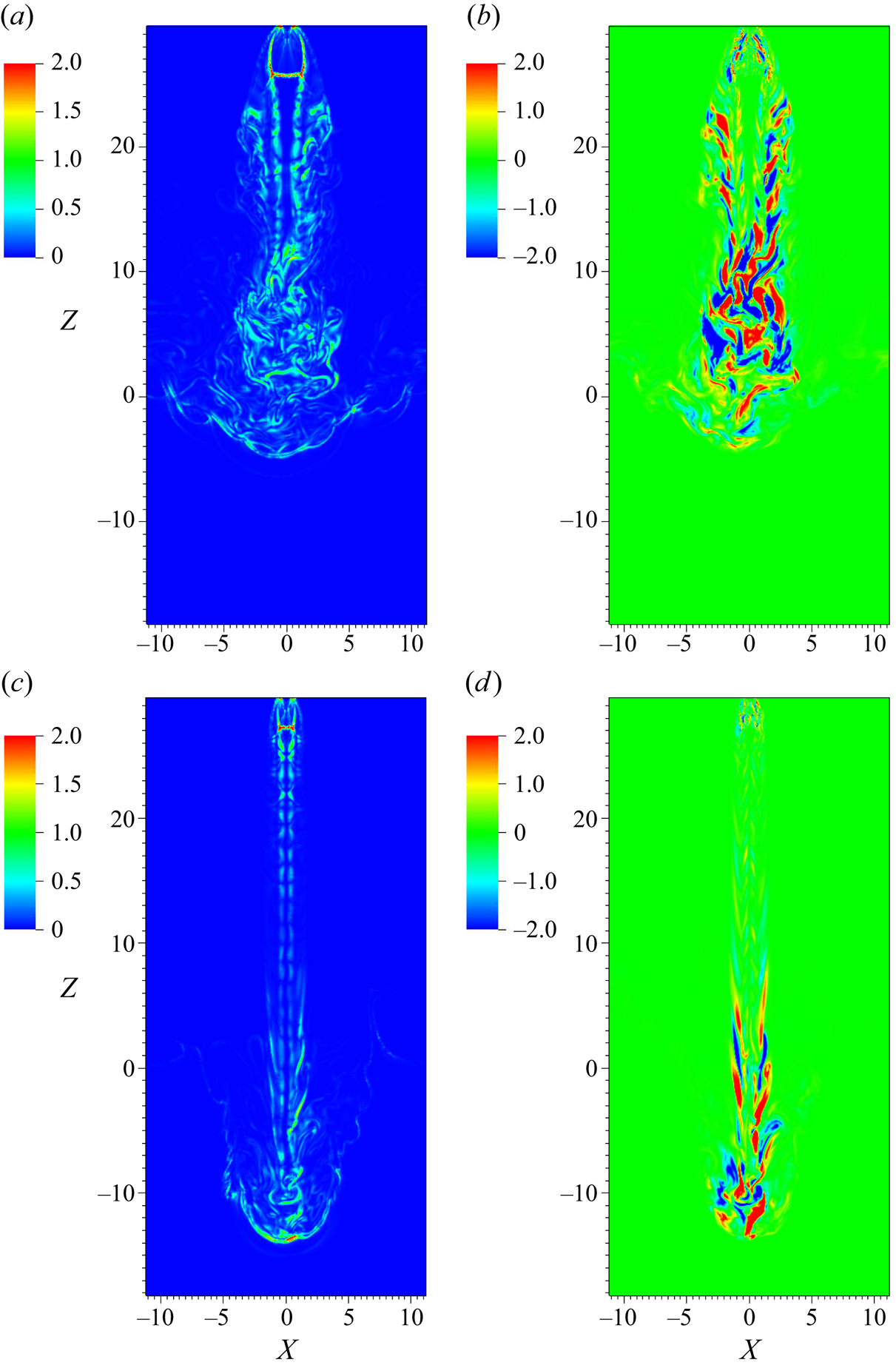
Instantaneous quantities of interest are  $\boldsymbol {\nabla }( \overline {\rho _{f} }/\overline {\alpha _{f}})$ and
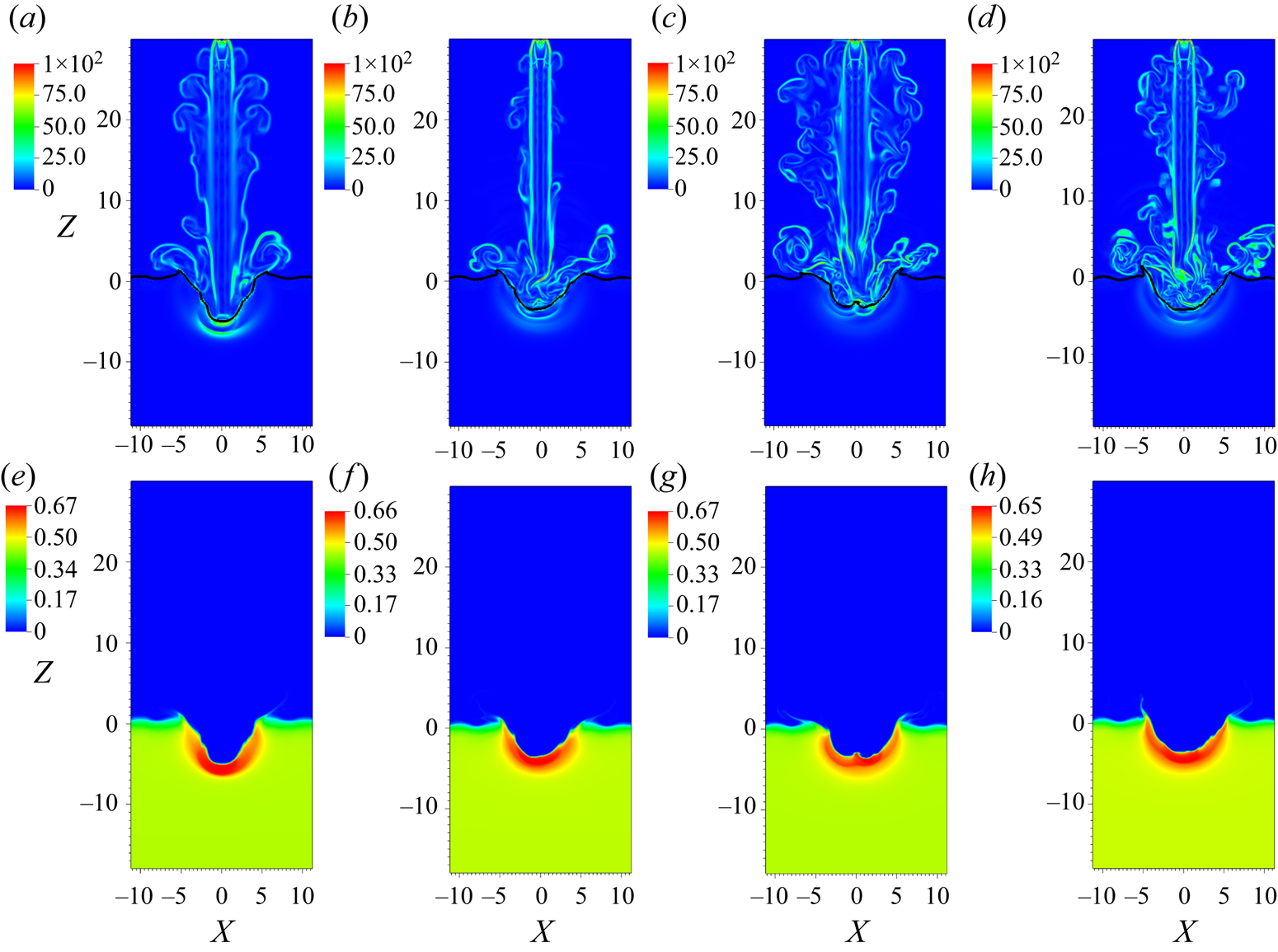
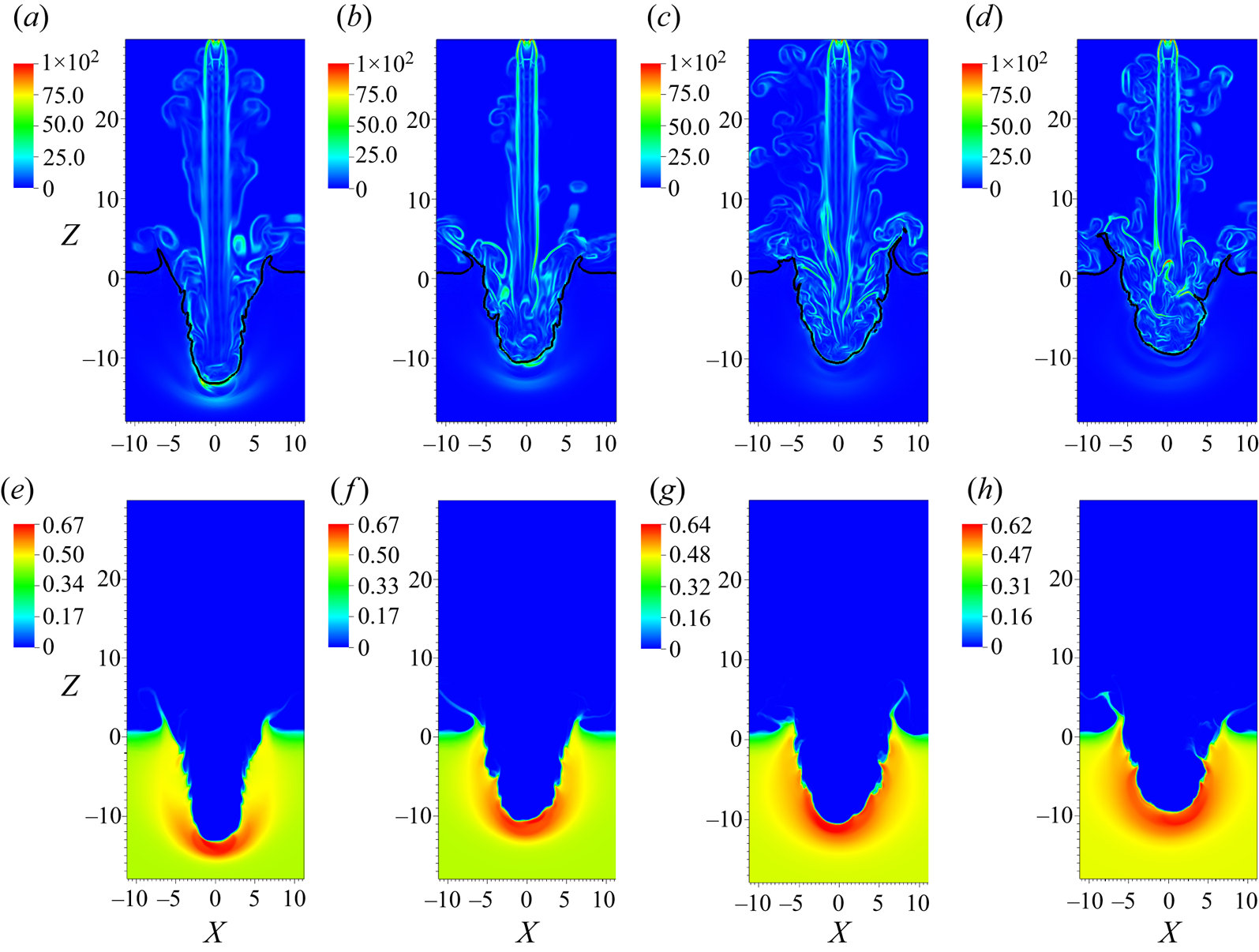
 $\overline {\alpha _{s}}$, as the former exemplifies turbulent structures, whereas the latter is a good indicator of crater shape and depth. Simulations of cases C3-G1, C3-G2, C3-G3 and C3-G4 from table 2 are conducted until
 $t^{\ast }\sim 120\text {--}145$, as a tentative range of stations at which a statistically steady-state rate of growth may have been achieved (to be examined below). Figure 2 illustrates
 $\boldsymbol {\nabla }( \overline {\rho _{f}}/\overline {\alpha _{f}})$ and
 $\overline {\alpha _{s}}$ at
 $t^{\ast } =69$ in the
 $(X,0,Z)$ plane. The large-scale turbulent structures are under-resolved in C3-G1 and C3-G2 relative to C3-G3 and C3-G4. As visually observed, C3-G3 and C3-G4 are qualitatively in better agreement with each other as far as the jet shape, crater depth and crater wall slopes. In figures 2(a)–2(d), the locus
 $\overline {\alpha _{s}}= 0.1$ (visible as a black curve) indicates the location of this locus with respect to the jet. In all cases, the locus is convoluted with folds representative of the hydrodynamic structures of the jet leaving a footprint on the granular bed, and this convoluted shape dynamically evolves as the crater develops in time.
Plots of  $(X,0,Z)$ plane views of
 $\boldsymbol {\nabla }( \overline {\rho _{f}} /\overline {\alpha _{f}})$ (a,b,c,d) and
 $\overline {\alpha _{s}}$ (e,f,g,h) for grids G1 (a,e), G2 (b,f), G3 (c,g) and G4 (d,h) at
 $t^{\ast } = 69$. The black contour line represents the locus
 $\overline {\alpha _{s}} =0.1$.

The same variables are depicted at  $t^{\ast } = 119$ in figure 3 for cases C3-G1–C3-G4. Strikingly similar qualitative features are observed for C3-G3 and C3-G4 that are different from C3-G1 and C3-G2. The
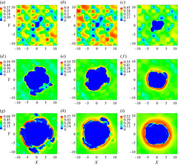
 $(X,Y,0)$ plane visualizations of
 $\overline {\alpha _{s}}$ for the craters obtained with C3-G1 – C3-G4 at
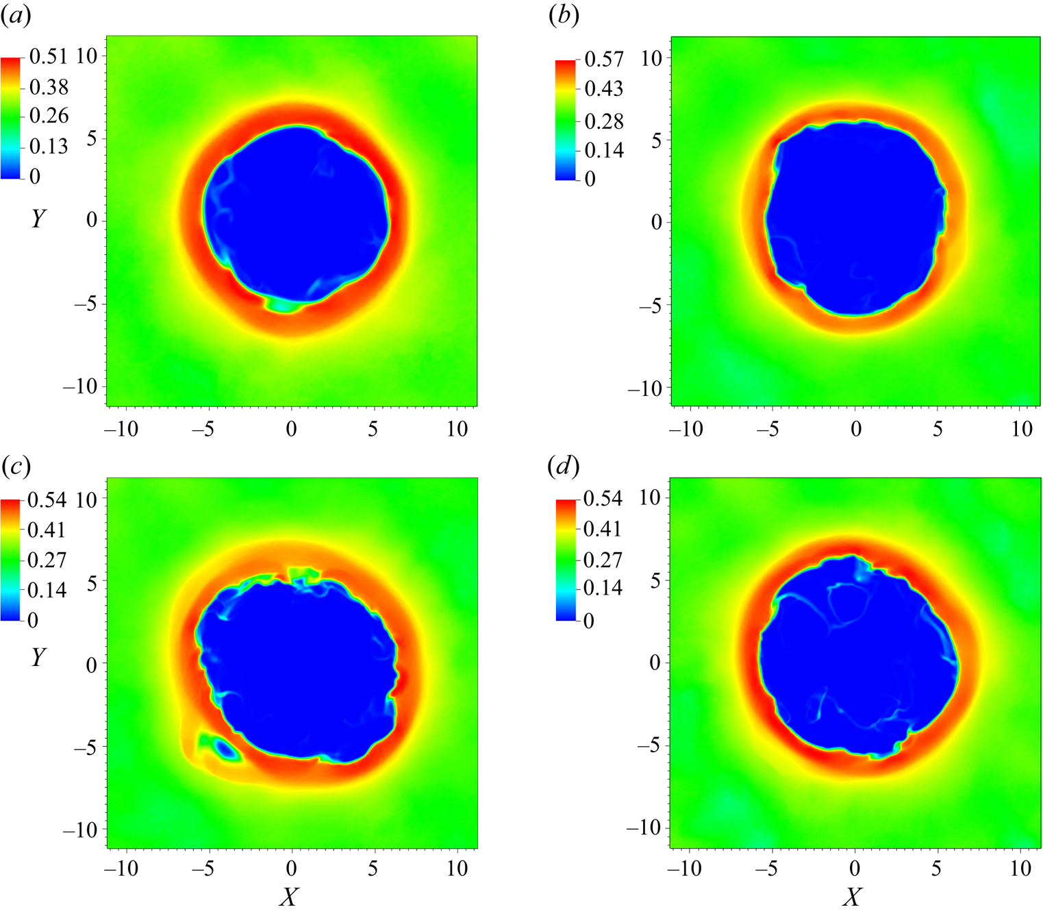
 $t^{\ast } = 119$ are portrayed in figure 4, showing that, despite detailed differences of the crater appearance, the crater diameter and rim thickness are similar for all four cases, suggesting grid convergence for this quantity.
Plots of  $(X,0,Z)$ plane views of
 $\boldsymbol {\nabla }( \overline {\rho _{f}} /\overline {\alpha _{f}})$ (a,b,c,d) and
 $\overline {\alpha _{s}}$ (e,f,g,h) for grids G1 (a,e), G2 (b,f), G3 (c,g) and G4 (d,h) at
 $t^{\ast } = 119$. The black contour line represents the locus
 $\overline {\alpha _{s} }=0.1$.

The  $(X,Y,0)$ plane view of
 $\overline {\alpha _{s}}$ for grids (a) G1, (b) G2, (c) G3 and (d) G4 at
 $t^{\ast } = 119$.

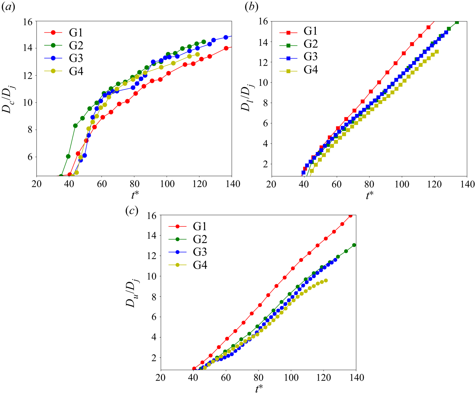
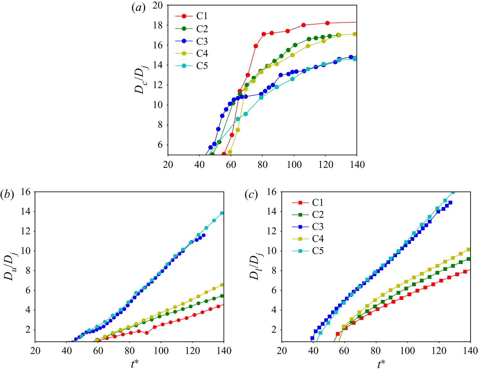
Important statistical quantities examined for grid convergence are the length scales indicated in figure 1(b). The crater diameter,  $D_{c}$, is computed in the
 $(X,Y,0)$ plane by first azimuthally averaging
 $\overline {\alpha _{s}}$ and then identifying the radial location of the maximum azimuthally averaged
 $\overline {\alpha _{s}}$. This location is in the compaction zone at the crater sidewalls and is defined as the crater edge, allowing the crater radius to be computed;
 $D_{c}$ is calculated as twice this radial distance. To compute the crater upper depth,
 $D_{u},$ the value of
 $\overline {\alpha _{s}}$ is again considered, but this time along the vertical axis,
 $(0,0,Z),$ from the centre of the jet exhaust plane to the bottom end of the simulation domain. Along this vertical line,
 $\overline {\alpha _{s}} = 0$ at the jet exhaust plane and stays null along the jet centreline up to the granular bed location where it increases due to compaction, reaching a value larger than the undisturbed bed
 $\overline {\alpha _{s}}$; below this compaction zone, the value of
 $\overline {\alpha _{s}}$ asymptotes to the undisturbed initial
 $\overline {\alpha _{s}}$ in the bed. By the present definition,
 $D_{u}$ is the location where
 $\overline {\alpha _{s}} =0.05$ is first encountered traversing vertically downward from the jet exhaust plane. Likewise, the crater lower depth,
 $D_{l}$ is defined as the location where
 $\overline {\alpha _{s}}$ is greater by 0.05 than the undisturbed initial value in the bed, now traversing vertically up from the bottom end of the simulation domain. While these definitions of
 $D_{u}$ and
 $D_{l}$ contain arbitrariness, they do capture the nature of these length scales and at the same time they provide quantitative statistical information to consistently evaluate and compare results of several simulations. Of particular interest is the time evolution of
 $D_{c}$,
 $D_{u}$ and
 $D_{l}$. For subsonic jets, there is evidence that crater diameters gradually widen with time (Metzger et al. Reference Metzger, Latta, Schuler and Immer2009), however, for supersonic jets the impingement shock results in a ‘splash stage’ characterized by the sudden formation of the crater, which is then followed by an ‘advection stage’ (Metzger et al. Reference Metzger, Smith and Lane2011) where the crater widens more gradually. During the splash stage, the crater walls experience high unsteadiness, being the result of initially formed structures eroding away. Because of this high unsteadiness, the azimuthal averaging was found to be meaningless in computing
 $D_{c}$,
 $D_{u}$ and
 $D_{l}$ during this stage, and therefore these quantities are only illustrated during the advection stage; since cases do not all reach the advection stage at the same
 $t^{\ast }$, a conservative approach is adopted and results are reported only past
 $t^{\ast }\simeq 40$. Figure 5(a) illustrates
 $D_{c}/D_{j}$, figure 5(b) depicts
 $D_{l}/D_{j}$ and figure 5(c) portrays
 $D_{u}/D_{j}$. Although results obtained with all simulations C3-G1–C3-G4 show the achievement of approximately the same asymptotic growth rate,
 $D_{c}/D_{j}$ has eventual similar values only for C3-G2–C3-G4. Additionally, the crater growth before reaching the asymptotic growth rate is similar only for C3-G3 and C3-G4. Apparent from figures 5(b) and 5(c), the information from examination of
 $D_{c}/D_{j}$ also applies to
 $D_{l}/D_{j}$ and
 $D_{u}/D_{j},$ and reinforces the choice of C3-G3 as the converged grid; and the simulation is further called C3. Since simulations C1, C2, C3, C4 and C5 are performed at approximately the same
 $Re$ value, the convergent grid for C3 (former C3-G3) is used for the remaining analysis.
Variation of crater-shape length scales with  $t^{\ast }$. (a)
 $D_{c}/D_{j};$ (b)
 $D_{l}/D_{j};$ (c)
 $D_{u}/D_{j}$.

4.2. Jet dynamics
4.2.1. Jet visualizations
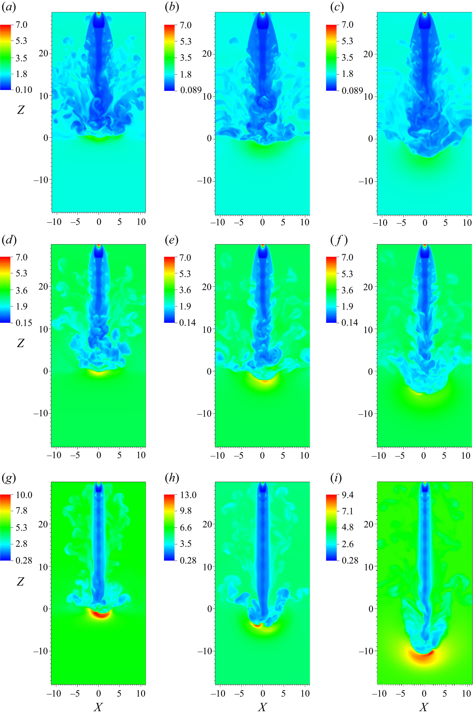
To characterize the jet shape as it leaves the nozzle and strikes the granular bed, the absolute fluid density,  $\overline {\rho _{f}}/\overline {\alpha _{f}}$, is selected as the pertinent variable. For cases C1, C2 and C3,
 $\overline {\rho _{f}}/\overline {\alpha _{f}}$ is presented in figure 6 at three different times upon the jet striking and penetrating the granular soil: early (
 $t^{\ast } = 50$), intermediate (
 $t^{\ast } = 74$) and late (
 $t^{\ast } = 124$). Figures 6(a)–6(c) indicate that the
 $t^{\ast }$ value corresponding to the time station when the jet strikes the soil is different according to the case. At
 $t^{\ast } = 50$, the jet has just reached the soil surface for C1, whereas it has already penetrated somewhat for C2; for C3, the penetration is more substantial than for C2. This is because jets C1, C2 and C3, which are in decreasing order of
 $\overline {\rho _{f}}/\overline {\alpha _{f}}$, spread less into the ambient from C1 to C3, and lose less momentum. Because of this aspect, it is important to make the comparison at several
 $t^{\ast }$ values. At early times the periphery of the jet develops mushroom-like structures that are caused by shear effects – very prominent for high-speed flows – between the jet and atmospheric fluid. These structures subside with time, as the jet penetrates the soil and assumes a column-like shape indicative of being more structurally coherent. At the base of the jet,
 $\overline {\rho _{f}}/\overline {\alpha _{f}}$ is larger as the jet strikes the granular bed, thus causing a stagnation region where the jet fluid accumulates. When the jet strikes the granular soil, a shear layer is formed that convects upward at an angle to the jet axis, representing a reverse flow. Clearly, with decreasing
 $\rho _{f,j}/\rho _{f,a}$ the indications through
 $\overline {\rho _{f}}/\overline {\alpha _{f}}$ are that the jet displays less turbulent structures at early times, a more coherent shape at late times, the formed reverse flow has a smaller angle with the jet axis, and there is increasing soil penetration. At same
 $\rho _{f,j}$ value, these differences result from the effect of
 $\rho _{f,a}$ (and fluid pressure) changing the jet potential core lengths, a fact which affects the jet/granular-bed interaction (see below), and thus the shape of the turbulent structures at the base of the jet that are directly influenced by the amount of momentum transferred to the granular bed particles.
Value of  ${\overline {\rho _{f}}}/{\overline {\alpha _{f}}}$ for cases C1 (a–c), C2 (d–f) and C3-G3 (g–i) at
 $t^{\ast } = 50$ (a,d,g), 74 (b,e,h) and 124 (c,f,i).

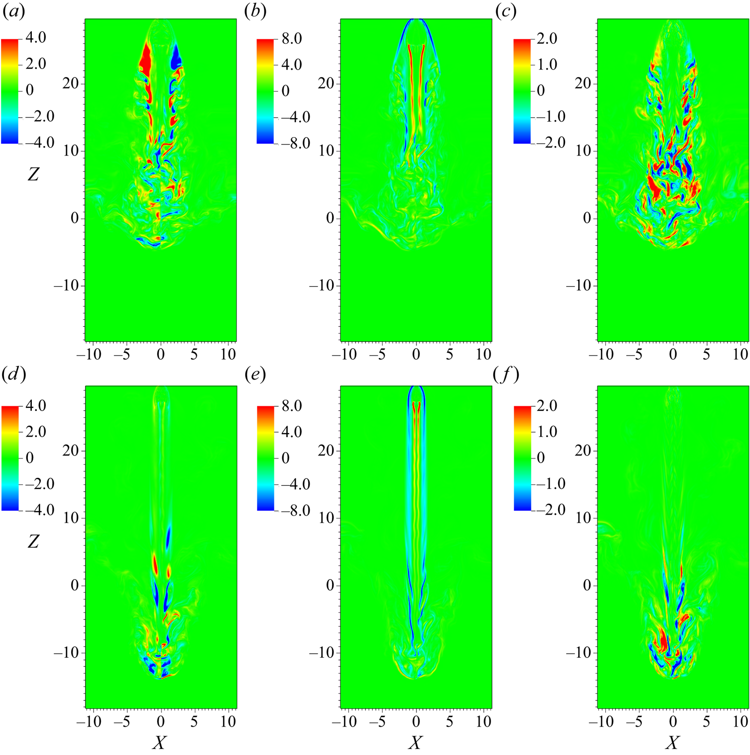
The non-dimensional vertical fluid velocity,  $\tilde {u}_{f,z}/a_{o}$, and
 $\hat {p}_{f}$ are depicted in figures 7(a–c) and 7(d–f), respectively, at
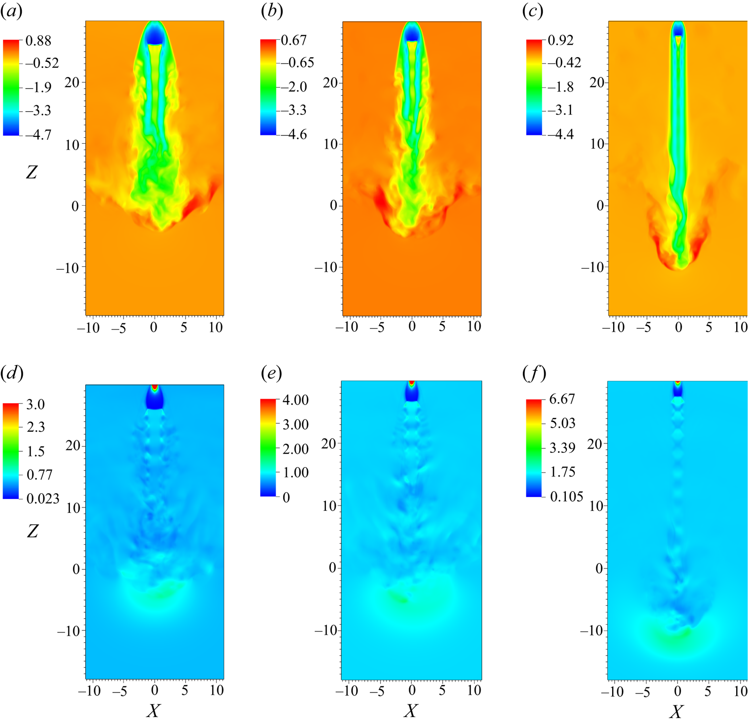
 $t^{\ast } = 124$ for cases C1, C2 and C3. Jet C3 has a distinctive column-like appearance compared to jet C1 and C2, due to the longer potential core, as previously mentioned. The velocity magnitude for the reverse flow in the vicinity of the base of the jet is highest for case C3 and is
 $\sim$180 m s
 $^{-1}$ (using the non-dimensionalizing ambient sound speed
 $a_{o} = 198$ m s
 $^{-1}$); such high fluid speeds could cause damage to a lander on the planetary surface. Mach diamonds, characteristic of supersonic jet flows, are evident in the
 $\hat {p}_{f}$ profiles (see figure 7d–f) and have different shapes for the different ambient conditions (see Wilcox et al. (Reference Wilcox, Weir, Nicholls and Dunlap1957) for more discussion). Overexpanded nozzles give rise to oblique shock waves at the nozzle exit which intersect and cause the Mach diamond pattern (Wilcox et al. Reference Wilcox, Weir, Nicholls and Dunlap1957). On the other hand, underexpanded nozzles will lead to Mach discs due to the focusing of compression waves from the boundaries of the jet (Wilcox et al. Reference Wilcox, Weir, Nicholls and Dunlap1957). If the underexpansion is sufficiently large, the oblique shocks are curved in shape, and this configuration is referred to in the literature as a shock bottle (Wilcox et al. Reference Wilcox, Weir, Nicholls and Dunlap1957). Mach discs are also observed a short distance away from the jet nozzle exhaust (see figure 7), since the flow from the nozzle is not perfectly expanded compared to the ambient; more details on Mach disc formation for supersonic jets can be found in Wilcox et al. (Reference Wilcox, Weir, Nicholls and Dunlap1957). Figures 7(d)–7(f) show that the size of the Mach diamonds is smaller and they are more numerous for case C3 compared to C1, which is a direct consequence of jet lateral expansion upon exhausting from the nozzle; this expansion depends on
 $\rho _{f,j}/\rho _{f,a}$ (and the corresponding pressure ratio) at the nozzle exhaust plane. These differences in the jet shape and structure are responsible for different crater shapes, as will be apparent in § 4.4.
Value of  $\tilde {u}_{f,z}/a_{o}$ (a–c) and
 $\hat {p}_{f}$ in bar units (d–f) for cases C1 (a,d), C2 (b,e) and C3 (c,f) at
 $t^{\ast } = 124$.

4.2.2. Jet spreading
A more complete understanding of the effect of  $\rho _{f,j}/\rho _{f,a}$ can be achieved by assessing the jet spreading and the entrainment into the jet. To better understand the effect of
 $\rho _{f,j}/\rho _{f,a}$ on jet shape and spreading, the first selected time for the analysis,
 $t^{\ast }=36$, corresponds to the time station when the jet barely strikes the granular bed, and thus the crater is yet to form. In § 4.4, an analysis of the subsequent crater evolution dependence on the shape of the jet produced by different values of
 $\rho _{f,j}/\rho _{f,a}$ is presented.
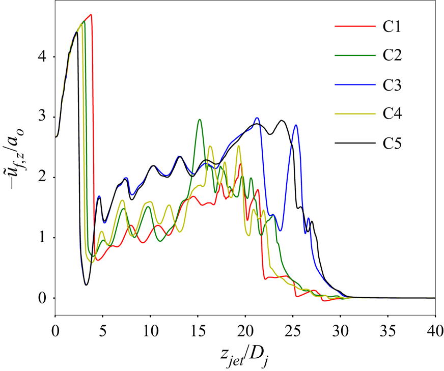
The instantaneous profile of  $-\tilde {u}_{f,z}$ at
 $t^{\ast } = 36$ for all cases is depicted in figure 8, as a function of
 $z_{jet}/D_{j}$, where
 $z_{jet}$ is measured vertically downward from the exhaust plane of the jet so that
 $z_{jet}=0$ denotes the jet exhaust plane and
 $z_{jet}=30D_{j}$ denotes the pristine soil (same plane as
 $Z=0$). Starting from the same value at the jet exhaust,
 $-\tilde {u}_{f,z}$ increases in the vicinity of the jet exhaust up to reaching the location of a Mach disk (near
 $z_{jet}/D_{j} = 4$) formed due to the physical discontinuity in the fluid density between the jet exhaust and the ambient; as discussed in § 4.2.1, Mach disks are formed since
 $\rho _{f,j}/\rho _{f,a}>1$ and thus the jet spreads into the atmosphere (see Wilcox et al. (Reference Wilcox, Weir, Nicholls and Dunlap1957) for more details on the physics of Mach disk formation). As the jet momentum in the axial direction decreases due to spreading in the lateral direction,
 $-\tilde {u}_{f,z}$ decreases substantially in the axial direction away from the nozzle exhaust plane. Further penetration into the atmosphere is determined by the concurrent processes of entrainment of the ambient fluid into the jet and jet lateral expansion that provoke an increase/decrease in
 $-\tilde {u}_{f,z}$ with
 $z_{jet}$; this process induces fluctuations in the
 $-\tilde {u}_{f,z}$ value, with the result that as the jet approaches the soil surface,
 $-\tilde {u}_{f,z}$ partially recovers from the decrease near the jet exhaust. Near the jet exhaust, i.e.
 $z_{jet}/D_{j}\lessapprox 2.5, -\tilde {u}_{f,z}/a_{o}$ is in magnitude largest for C1, than for C2 and C4, and finally for C3 and C5, indicating that the value of
 $\rho _{f,j} /\rho _{f,a}$ controls this near-exhaust region. The reduction in
 $-\tilde {u}_{f,z}$ past
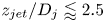 $z_{jet}/D_{j}\lessapprox 2.5$ is largest for C3 and C5, intermediary for C2 and C4, and smallest for C1, supporting again the idea that these processes are dominated by the
 $\rho _{f,j}/\rho _{f,a}$ value as the extent of lateral expansion of the jet is determined by this density ratio. Past
 $z_{jet}/D_{j}\approx 3$ and up to
 $z_{jet}/D_{j}\approx 22,$ the magnitude of
 $-\tilde {u}_{f,z}/a_{o}$ is largest for C3 and C5, then for C2 and C4, with the smallest one being C1; thus, up to
 $z_{jet}/D_{j} \approx 22,$ the influence of
 $\rho _{f,j}/\rho _{f,a}$ prevails in determining the magnitude of
 $-\tilde {u}_{f,z}/a_{o}.$ In the region
 $z_{jet} /D_{j}\approx 22\text {--}25$, it appears that nonlinear effects due to the aforementioned reverse flow (formed when jet strikes the soil) are at play as it is clear that, because
 $-\tilde {u}_{f,z}\!\neq 0$ near
 $z_{jet}/D_{j} = 30$ (i.e. stagnation zone), the fluid in the jet has penetrated into the soil. Finally, shortly past
 $z_{jet}/D_{j}\approx 30,$ for all cases
 $-\tilde {u}_{f,z}/a_{o}$ asymptotes to zero, as expected.
Value of  $-\tilde {u}_{f,z}/a_{o}$ at
 $t^{\ast } = 36$ for cases C1–C5.

To calculate jet spread, a transformation of coordinates  $(x,y,z)\rightarrow (r,\theta ,z)$ is implemented such that
 \begin{equation} \boldsymbol{e}_{r}=\boldsymbol{e}_{x}{\rm cos}\theta+\boldsymbol{e}_{y}{\rm sin}\theta; \boldsymbol{e}_{\theta}={-}\boldsymbol{e}_{x}{\rm sin}\theta+\boldsymbol{e}_{y}{\rm cos}\theta, \end{equation}
where  $\boldsymbol {e}_{x}, \boldsymbol {e}_{y}, \boldsymbol {e}_{r}, \boldsymbol {e}_{\theta }$ are unit normal vectors in the
 $x$,
 $y$,
 $r$ and
 $\theta$ directions, respectively; the resulting velocity field is (
 $\tilde {u}_{f,r} ,\tilde {u}_{f,\theta },\tilde {u}_{f,z}$). Azimuthally averaged velocities, e.g.
 $\langle \tilde {u}_{f,r}\rangle ,$ are computed as follows: at each specified
 $z,$ the
 $\tilde {u}_{f,r}$ values are placed into bins in the
 $r$ direction; thus the number of samples available in each given bin at each specified
 $z$ is known. Performing an azimuthal average nulls
 $\langle \tilde {u}_{f,\theta }\rangle$ but will result in non-null
 $\langle \tilde {u}_{f,r}\rangle$ and
 $\langle \tilde {u}_{f,z}\rangle$; all root mean square (r.m.s.) values of the variables are also non-null.
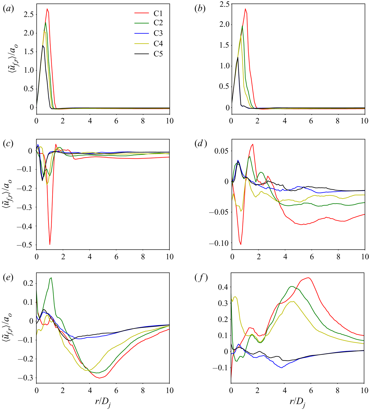
Figure 9 illustrates  $\langle \tilde {u}_{f,r} \rangle /a_{o}$ as a function of
 $r/D_{j}$ at
 $t^{\ast } = 36$ at different vertical distances
 $D_{j}\leq z_{jet}\leq$ 20
 $D_{j}.$ Up to
 $z_{jet} = 5 D_{j}$, the action is concentrated closer to the centre of the jet. For
 $z_{jet} = D_{j}$ and
 $2 D_{j}$, the jet expansion increases with the
 $\rho _{f,j}/\rho _{f,a}$ value. For
 $z_{jet} = 5D_{j}$,
 $\langle \tilde {u}_{f,r}\rangle /a_{o}<0$, indicating entrainment of the atmospheric fluid into the jet, and this phenomenon is more pronounced for C1, the same for C3 and C5, and similar for C2 and C4. At further vertical distances from the jet exhaust, the jet dynamics becomes more complex. At
 $z_{jet} = 10D_{j}$, the entrainment region has moved closer to the jet centreline; C1 and C4 jets experience entrainment into the jet whereas C2, C3 and C5 experience jet expansion. The magnitude of
 $\langle \tilde {u}_{f,r}\rangle /a_{o}$ is still largest for C1 than C4, and similar for C2, C3 and C5. Past
 $r/D_{j}\gtrsim 1$ and up to 4, other than
 $\rho _{f,j}/\rho _{f,a}$ effects are at play, but past
 $r/D_{j}\gtrsim 4$ the value of
 $\rho _{f,j}/\rho _{f,a}$ again dominates the jet behaviour with the magnitude of
 $\langle \tilde {u}_{f,r}\rangle /a_{o}$ being larger for more elevated
 $\rho _{f,j}/\rho _{f,a}$ values. At
 $z_{jet}/D_{j} =15$, past
 $r/D_{j}\gtrsim 2.5$ the jet characteristics have the same alignment with
 $\rho _{f,j}/\rho _{f,a}$ as at
 $z_{jet}/D_{j} =10.$ Finally, at
 $z_{jet}/D_{j} =20,$ past
 $r/D_{j}\gtrsim 2$ there is a qualitative change between both C3 and C5 for which there is entrainment into the jet due to the
 $\rho _{f,j}/\rho _{f,a}$ value being close to unity, and all C1, C2 and C4 jets, which expand into the ambient due to the
 $\rho _{f,j}/\rho _{f,a}$ value being larger than 2. Among expanding jets, jet C1 expands the most and jet C4 expends the least, aligning with the decreasing value of
 $\rho _{f,j} /\rho _{f,a}.$
Value of  $\langle \tilde {u}_{f,r}\rangle /a_{o}$ at
 $t^{\ast } = 36$ at different vertical distances from the jet exhaust plane: (a)
 $D_{j}$; (b) 2
 $D_{j}$; (c) 5
 $D_{j}$; (d) 10
 $D_{j}$; (e) 15
 $D_{j}$; (f) 20
 $D_{j}$.

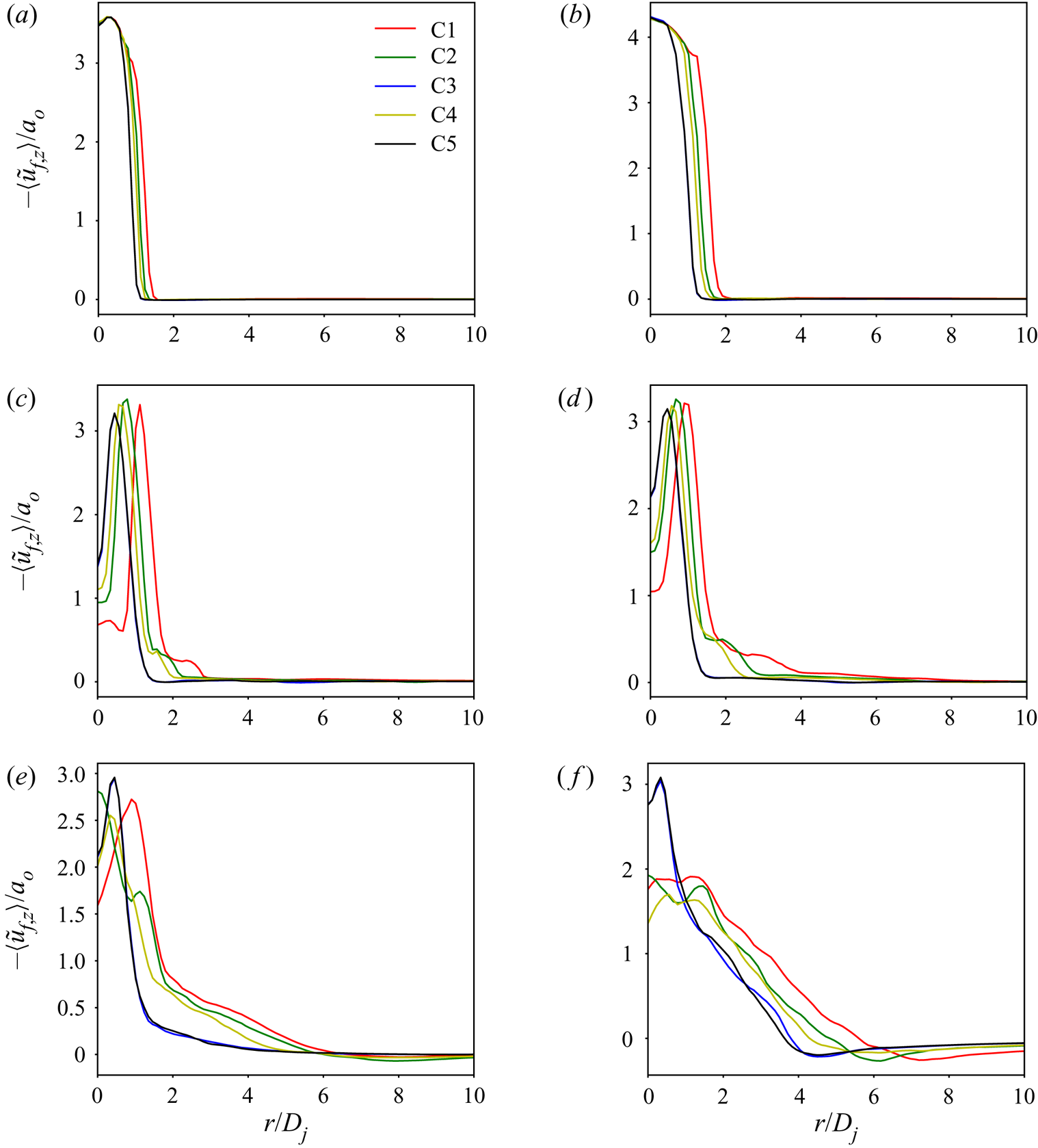
The variation of  $-\langle \tilde {u}_{f,z}\rangle /a_{o}$ at
 $t^{\ast } = 36$ at different
 $z_{jet}/D_{j}$ values is portrayed for all cases in figure 10 as a function of
 $r/D_{j}$. The larger jet spreading with increasing
 $\rho _{f,j}/\rho _{f,a}$ is again substantiated. Near the jet exhaust, the centreline (
 $r = 0$) values of
 $\langle \tilde {u} _{f,z}\rangle$ are nearly identical as the entrainment of the ambient fluid into the jet is negligible at those locations. However, at
 $z_{jet}/D_{j} = 5$, 10 and 15, the centreline
 $\langle \tilde {u}_{f,z}\rangle$ magnitude is larger for C3 and C5 that almost coincide, followed by C2 and C4 that are similar and lastly by C1. This is due to a larger jet spreading which leads to a relatively smaller momentum and energy near the jet centreline. A smaller
 $\rho _{f,j}/\rho _{f,a}$ jet will maintain a larger
 $-\langle \tilde {u}_{f,z}\rangle /a_{o}$ near the centreline and will expand the jet less into the atmosphere.
Value of  $-\langle \tilde {u}_{f,z}\rangle /a_{o}$ at
 $t^{\ast } = 36$ at different vertical distances from the jet exhaust plane: (a)
 $D_{j}$; (b) 2
 $D_{j}$; (c) 5
 $D_{j}$; (d) 10
 $D_{j}$; (e) 15
 $D_{j}$; (f) 20
 $D_{j}$.

Considering the azimuthally averaged r.m.s. of the velocity vector  $\tilde {\boldsymbol {u}}_{f}$ at
 $t^{\ast } = 36$ at different
 $z_{jet}$ (not shown), vertically up to
 $z_{jet}/D_{j}=2$, the action is confined for all jets near the centreline region,
 $r/D_{j}\lesssim 2,$ with C1 exhibiting the largest values, and C3 and C5 showing the smallest values. At
 $z_{jet} /D_{j}=5,$ the action spreads to
 $r/D_{j}=3$ and there is the same alignment with the
 $\rho _{f,j}/\rho _{f,a}$ value as observed at
 $z_{jet}/D_{j}=2.$ An adjustment in the centreline region appears at
 $z_{jet}/D_{j}=10$ and 15 in that the C2 and C4 jets display the largest values, followed by C1 and then by the similar C3 and C5 values, while far from the centreline the alignment with the
 $\rho _{f,j}/\rho _{f,a}$ value prevails. Finally, for
 $z_{jet}/D_{j}=20,$ at virtually all radial locations the C1 jet is the most turbulent, followed by the similar levels of turbulence in C2 and C4, and lastly by C3 and C5 having the same, weakest turbulence characteristics. Basically, among all jets, the largest expansion of the C1 jet into the atmosphere promotes a more turbulent behaviour.
4.3. Species spatial distribution in the jet
The species in the jet are neither reacting nor is there an emanation of species from the soil. Thus, in fluid mechanics terms these species constitute passive scalars which are typically used to understand the mixing between jet and atmospheric fluid. For example, Balakrishnan & Bellan (Reference Balakrishnan and Bellan2019) found that both regular and uphill species diffusion occurs in the jet for Titan-like atmospheres. In addition, the role of the molecular mass of different jet species on the ensuing crater formation was documented. In the present study, the focus is on turbulent mixing of the species.
Both  $Y_{H_{2}O}$ and
 $Y_{N_{2}}$ are illustrated in the
 $(X,0,Z)$ plane at
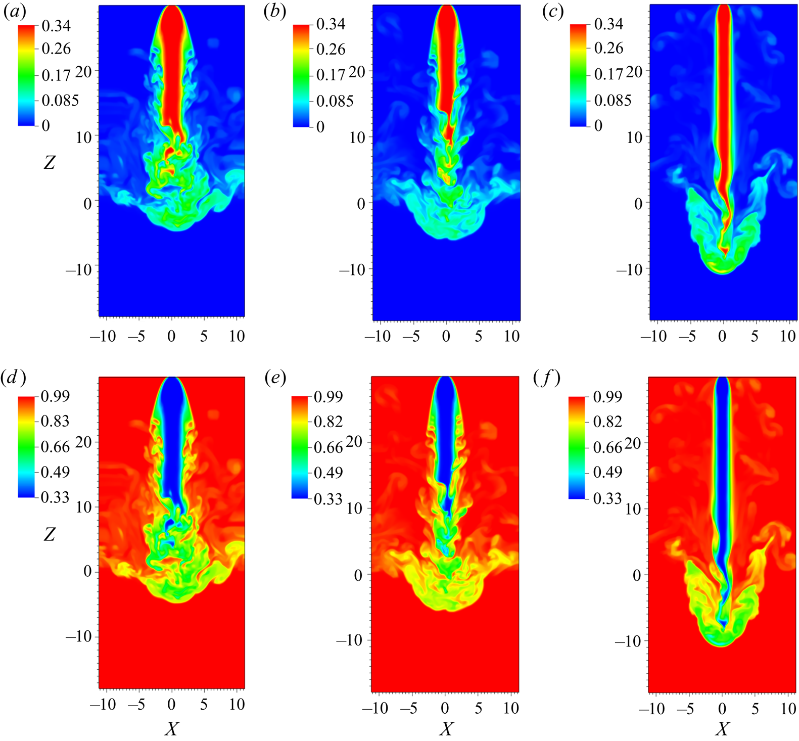
 $t^{\ast } = 124$ for cases C1, C2 and C3 in figure 11. Three distinct regions of turbulent mixing are evident, each of which has a different physical mechanism governing it. The first region of turbulent mixing occurs at the jet periphery, a short distance away from the jet exhaust plane (near
 $Z\sim$ 10–20) for jets C1 and C2 only, but not for jet C3. As already discussed, for larger
 $\rho _{f,j}/\rho _{f,a}$, i.e. case C1, the greater density differences between the jet and ambient fluids results in faster growth of hydrodynamic instabilities on the periphery of the jet, which subsequently break down to zones of turbulent mixing. For cases C1 and C2, these turbulent mixing zones are evident much closer to the jet exhaust plane, even before the end of the potential core. For case C3, however, due to the relatively smaller
 $\rho _{f,j}/\rho _{f,a}$ ratio, these jet-peripheral turbulent mixing zones appear only near to the end of the potential core (near
 $Z\sim$ 0–7). Furthermore, the scale of the turbulent structures is smaller for jet C1, of intermediate size for C2 and is larger for C3, as the onset of turbulence occurs in the same order with respect to the jet exhaust (C1, then C2 and finally C3).
Mass fractions  $Y_{H_{2}O}$ (a–c) and
 $Y_{N_{2}}$ (d–f) for cases C1 (a,d), C2 (b,e) and C3 (c,f) at
 $t^{\ast } = 124$.

The second mixing zone occurs at the base of the jet, and close to the jet centreline rather than on the jet periphery. Upon impinging the soil, the potential core eventually breaks up, giving rise to the second turbulent mixing zone. In this region, it is evident that the jet and atmospheric fluids mix over a wider region for jet C1 than jets C2 and C3; this is attributed to the shorter potential core length for jet C1 that results in mixing of the jet and atmospheric species nearer to the jet exhaust plane for case C1. This mixing region is strongly influenced by the shear effects which depend on the  $\rho _{f,j}/\rho _{f,a}$ value.
The third mixing zone is created by the downward moving jet interacting with the reverse flow created by the jet fluid bouncing off the particle bed. Since these two fluid streams have opposite velocities, shear effects are prominent, giving rise to the characteristic mushroom-like structures evident on the jet periphery. For case C3, the coherent structures in this reverse flow (figure 11f) are the site of intense species mixing as the jet flow and the reverse flow interaction creates shear layers; these shear layer structures are reminiscent of shear-induced instabilities. The angle between the jet flow axis and the reverse-flow axis differs according to the case; for cases C1 and C2, the angle is approximately 45 $^{\circ} $ from the jet axis, however, for case C3 the angle is only approximately 30
 $^{\circ} $. Thus, the
 $\rho _{f,j}/\rho _{f,a}$ value not only influences the timing of the creation of the reverse flow, but also affects the shape of the mixing region.
4.4. Crater characteristics
The observation that the jet dynamics is controlled by the  $\rho _{f,j} /\rho _{f,a}$ value allows restricting of the detailed analysis of crater characteristics to cases C1, C4 and C5, as the C2 jet is expected to produce a crater similar to that of C4 and distinct from C1, C3 and C5, and the C3 jet is foreseen to produce a crater similar to that of C5 and distinct from C1, C2 and C4. General comparisons between craters C3 and C5 highlight the influence of
 $\rho _{f,j}$ at the same
 $\rho _{f,j}/\rho _{f,a}$ value, whereas comparisons between C3 and C4 also indicate the effect of
 $\rho _{f,j}$ but now at the same
 $\rho _{f,a}$ value, albeit different values of
 $\rho _{f,j}/\rho _{f,a}.$
4.4.1. Crater dynamics
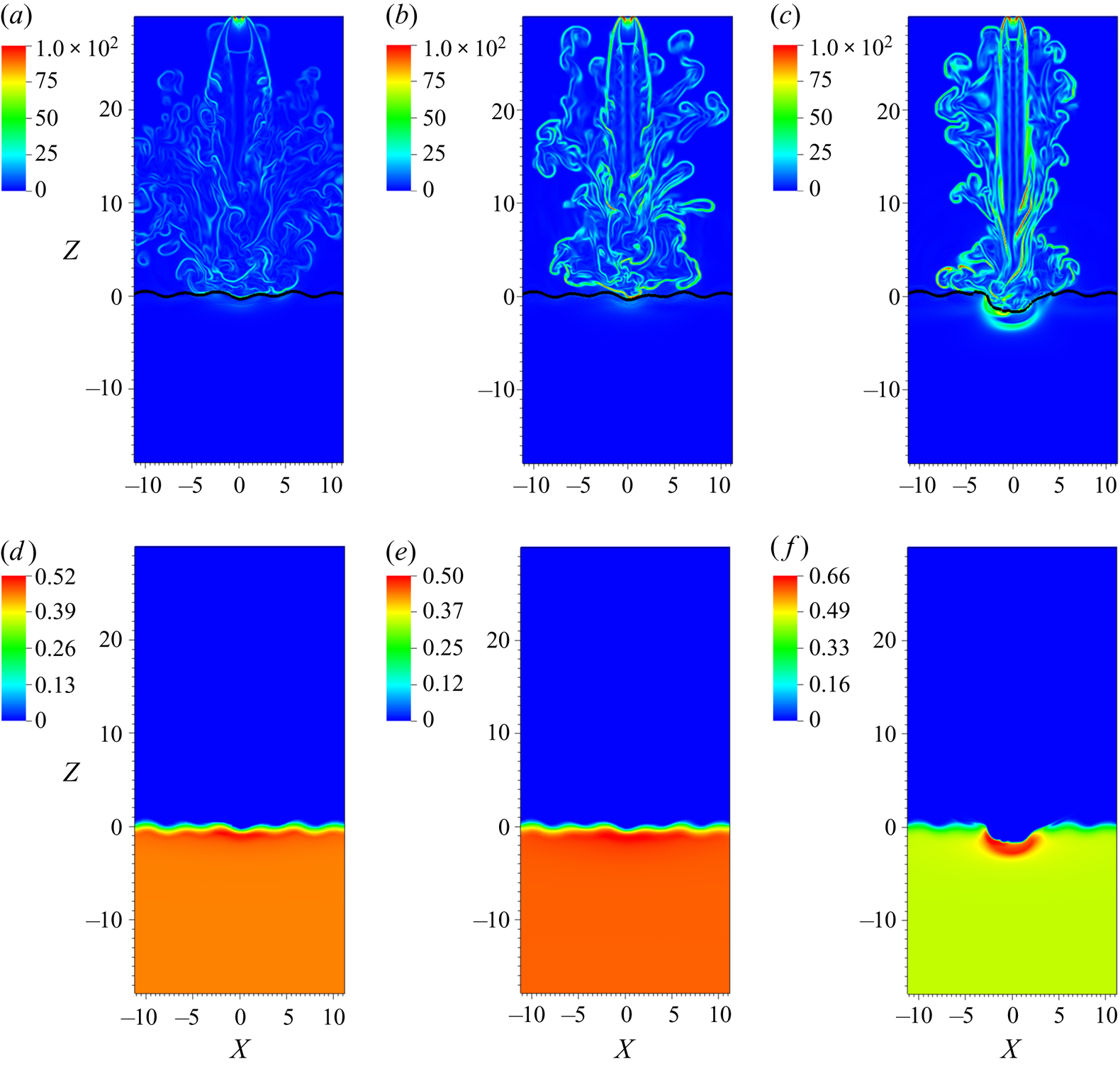
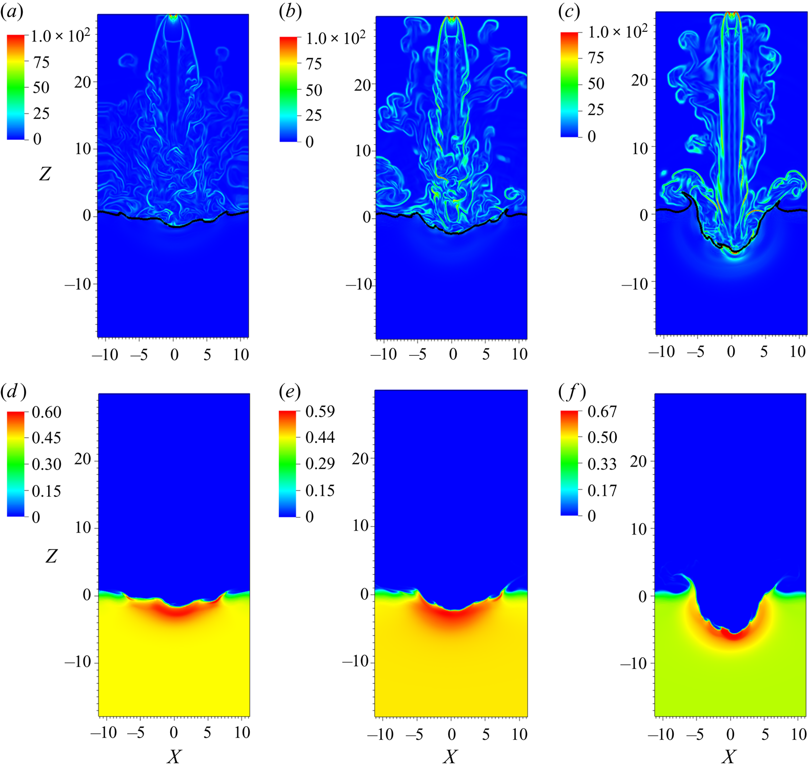
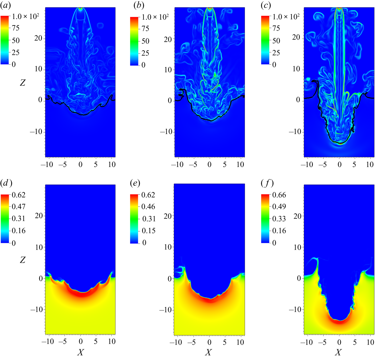
The crater formation due to jets C1, C4 and C5 is illustrated at different times,  $t^{\ast }=50,74$ and 124, in figures 12, 13 and 14, respectively. Just as in the illustrations of § 4.1,
 $\boldsymbol {\nabla }\overline {\rho _{f}}/\overline {\alpha _{f}}$ is selected as representative of the jet shape and it is juxtaposed to
 $\overline {\alpha _{s}}$ which visualizes the crater shape in the
 $(X,0,Z)$ plane. Jet C1 immediately spreads into the atmosphere as it enters it (i.e. close to the jet exhaust) and by so doing loses vertical momentum; by the time it arrives at the soil surface the jet has a blunt front which, combined with the reduced vertical momentum, results in it penetrating marginally the soil at
 $t^{\ast }=50$. At the other extreme, jet C5, which has the longest potential core among all cases, presents to the soil a pointed shape, and the combination of the larger momentum and more adept front shape is instrumental in a deeper soil penetration. Case C4 is intermediary between C1 and C5. The locus
 $\overline {\alpha _{s}} = 0.1$ in figures 12(a)–12(c), 13(a)–13(c) and 14(a)–14(c) is indicative of the displacement of the soil with respect to its initial location. At early times, the locus
 $\overline {\alpha _{s}} = 0.1$ is nearly horizontal, but becomes convoluted once the jet strikes the particle bed and follows the jet boundary.
Plots of  $(X,0,Z)$ plane views of
 $\boldsymbol {\nabla }( \overline {\rho _{f}} /\overline {\alpha _{f}})$ (top row) and
 $\overline {\alpha _{s}}$ (bottom row) for cases C1 (a,d), C4 (b,e) and C5 (c,f) at
 $t^{\ast } = 50$. The black contour line represents the locus
 $\overline {\alpha _{s}}=0.1$.

Plots of  $(X,0,Z)$ plane views of
 $\boldsymbol {\nabla }( \overline {\rho _{f}} /\overline {\alpha _{f}})$ (top row) and
 $\overline {\alpha _{s}}$ (bottom row) for cases C1 (a,d), C4 (b,e) and C5 (c,f) at
 $t^{\ast } = 74$. The black contour line represents the locus
 $\overline {\alpha _{s}}=0.1$.

Plots of  $(X,0,Z)$ plane views of
 $\boldsymbol {\nabla }( \overline {\rho _{f}} /\overline {\alpha _{f}})$ (top row) and
 $\overline {\alpha _{s}}$ (bottom row) for cases C1 (a,d), C4 (b,e) and C5 (c,f) at
 $t^{\ast } = 124$. The black contour line represents the locus
 $\overline {\alpha _{s}}=0.1$.

At  $t^{\ast }=74,$ the crater formed by jet C1 is shallow, and it appears that craters increase in depth with decreasing
 $\rho _{f,j}/\rho _{f,a}$ value. By
 $t^{\ast }=124,$ the crater cross-section shapes are well established and very distinct, directly corresponding to the shape of the impinging jet. Crater C1 has a parabolic cross-section, is shallow and outside the primary compaction zone and rim, which show some limited material expulsion through bursts, there is a secondary, shallower crater surrounding the primary crater; the rim of this secondary crater exhibits more substantial material expulsion through bursts. This secondary crater is attributed to the shear on the soil surface caused by the reverse flow formed when the jet strikes the soil, as discussed in § 4.2.1, and that moves upward at an angle from the jet axis. That is, when the angle of this reverse flow to the jet axis is large, as in case C1, the reverse flow shears the soil surface further away from the jet vicinity, and creates a secondary crater. Crater C4 has also a parabolic cross-section, but is deeper than crater C1, and the secondary crater is greatly reduced, surviving as only a hint; the expulsion of material through bursts is considerably enhanced with respect to crater C1. Finally, crater C5 has a conical cross-section shape instead of a parabolic shape, with substantially augmented expulsion of material from the rim with respect to crater C4. Compared to craters C1 and C4, ripples are evident on the inner crater wall that have been traced by Balakrishnan & Bellan (Reference Balakrishnan and Bellan2019) to shear from the reversed flow forming at larger depths than for C1 and C4, as discussed in § 4.2.1. Thus, it is clear that the
 $\rho _{f,j}/\rho _{f,a}$ value determines the crater cross-section shape: parabolic craters correspond to large values of
 $\rho _{f,j}/\rho _{f,a}$ whereas conical craters correspond to near unity values of
 $\rho _{f,j}/\rho _{f,a}.$
To inquire about the influence of  $\rho _{f,j}$ on crater formation and cross-section shape at a fixed
 $\rho _{f,j}/\rho _{f,a}$ value, cases C3 and C5 were comparatively analysed (not shown). Crater C5 is deeper than C3 due to the corresponding increase in the jet momentum (or equivalently
 $\rho _{f,a}$), and its walls are somewhat steeper due to the smaller angle between the reverse flow when the jet maintains higher core momentum, as it does at larger
 $\rho _{f,j}.$ The ripples on the crater wall are deeper for C5 compared to C3, a fact which is attributed to the increased turbulence produced by a higher-momentum jet when impinging a surface. Comparison of craters C3 and C4 also indicates the influence of
 $\rho _{f,j}$ but now at the same
 $\rho _{f,a}$ value (not shown), albeit different
 $\rho _{f,j}/\rho _{f,a}$ values. Both craters are parabolic, and the deeper crater is that having the larger
 $\rho _{f,j}.$ Thus, the conclusion is that the
 $\rho _{f,j}/\rho _{f,a}$ value determines the crater cross-section shape, and that the value of
 $\rho _{f,j}$ determines the crater depth.
Views of  $\overline {\alpha _{s}}$ in the
 $(X,Y,0)$ plane are presented in figure 15 for cases C1, C4 and C5 at
 $t^{\ast }=50,74$ and 124. Because jet C1 expands substantially into the atmosphere, the ensuing loss of concentrated momentum results in a shallow crater of a random top-view shape (see figure 15d,g). The lack of coherent crater shape in the
 $(X,Y,0)$ plane is manifested in a formed primary crater surrounded, and sometimes distorted, by several mini craters; there are thin compacted zones of granular particles separating the central main crater and the other mini craters (see figure 15g). At the other extreme is crater C5, formed by a jet carrying substantial momentum near its axis; the result is a more circular – i.e. coherent – crater; mini craters may be formed, but they are ephemeral, unlike for crater C1, and become consumed by the primary crater as the momentum from the jet compacts the soil particles. This transient phenomenon of mini-crater formation was explained in Balakrishnan & Bellan (Reference Balakrishnan and Bellan2019) (also termed ‘crater-in-a-crater’) by the temporary footprint left on the granular bed upon impingement from the jet. Crater C4 is intermediary between C1 and C5 in that the top-view shape of the primary crater is more circular, the number of mini craters is reduced with respect to crater C1, but the mini craters are not eventually consumed, unlike crater C5. Such mini craters are also visible in a field test experimental study of Metzger et al. (Reference Metzger, Smith and Lane2011), particularly figure 15 of Metzger et al. (Reference Metzger, Smith and Lane2011) in which multiple craters in a single larger crater are observed. Since only three-dimensional high-fidelity numerical simulations can resolve the energy-containing turbulent structures, these simulations are the only type that can capture these realistic phenomena. Models that have either low fidelity or are two-dimensional (e.g. the model of LaMarche et al. Reference LaMarche, Moran, van Wachem and Curtis2017) will not capture the true nature of the turbulent structures in the jet (see § 4.5 ) and thus the phenomenon of mini-crater formation may not be predicted.
Plots of  $(X,Y,0)$ plane views of
 $\overline {\alpha _{s}}$ for cases C1 (a,d,g), C4 (b,e,h) and C5 (c,f,i) at
 $t^{\ast } = 50$ (a–c), 74 (d–f) and 124 (g–i).

At  $t^{\ast }=124$ crater C3 (not shown) resembles crater C5 except that there are still surviving mini craters, and case C3 (not shown) and C4 are distinguished by the larger primary C4 crater as well as the larger mini crater. Thus, the value of
 $\rho _{f,j}/\rho _{f,a}$ affects the top-view form of the crater, with more coherent shapes visible for values closer to unity, and random shapes of a primary crater accompanied by the formation of mini craters for larger values of
 $\rho _{f,j}/\rho _{f,a}.$ At constant
 $\rho _{f,j}/\rho _{f,a}$ value, the magnitude of
 $\rho _{f,j}$ seems to influence the effective crater diameter. In all cases, the peak values of
 $\overline {\alpha _{s}}$ are still below the close packing limits (
 $\sim$ 0.65), as the
 $p_{fric}$ term in the momentum equation offers resistance to compaction beyond a certain limit. The compacted crater walls appear thinner for craters C1, C2 (not shown) and C4 than for craters C3 (not shown) and C5 for which the deeper penetration of the jet fluid into the granular bed makes the compacted zone of the crater walls thicker. However, a quantitative test is necessary to make these comparisons, as described next.
4.4.2. Crater diameter and depth
Considering that all craters have somewhat random shapes, the unified and systematic way of computing  $D_{c}$,
 $D_{u}$ and
 $D_{l}$, as explained in § 4.1, takes additional importance. For the high-density-fluid supersonic C1–C5 jets, the early time crater formation is sudden due to the high momentum of the jet fluid, and thus the crater widens more gradually with time than in subsonic jets, as more fluid accumulates inside the crater and later expands outwards. As already explained in § 4.1, this part of crater development is termed the ‘advection stage’ (Metzger et al. Reference Metzger, Smith and Lane2011), and
 $D_{c}$,
 $D_{u}$ and
 $D_{l}$ are only computed during the advection stage; the results are illustrated in figure 16 for all craters.
Crater length scales: (a)  $D_{c}/D_{j}$; (b)
 $D_{u}/D_{j}$; (c)
 $D_{l}/D_{j}$ for cases C1–C5.

According to the information in figure 16, among all craters, C1 is the second latest to initiate growth due to the large jet expansion into the ambient and the necessary time to build momentum in the jet core through atmospheric-fluid entrainment. However, once the crater is initiated, its rate of growth surpasses that of all other craters, resulting in the largest  $D_{c}$ (figure 16a). This largest
 $D_{c}$ is attributed to the reverse flow created upon the jet impinging the soil that, according to the discussion in § 4.4.1, is responsible for generating a secondary crater surrounding the primary central crater which results from the jet impingement. For large
 $\rho _{f,j}/\rho _{f,a},$ the large angle of the reverse flow with the jet axis is responsible for originating and continuing the secondary crater formation, finally leading to a shallow and large crater. Indeed, both
 $D_{u}$ (figure 16b) and
 $D_{l}$ (figure 16c) are the smallest crater depths among all of the craters. After the initial large growth rate of crater C1, the growth diminishes as the jet has penetrated the soil and the reverse flow, being mostly located within the crater depth, cannot affect very much the crater enlargement. After this time station, the crater grows at a substantially slower rate. Thus, one can identify a two-stage growth for
 $D_{c}$: an early time very rapid growth in which both the jet and the reverse flow play a role, and a later time slow growth when the jet has sufficiently penetrated the soil so that the reverse flow has minor effect.
Craters C1, C2 and C4 display the two-stage crater growth. Figure 16(a) shows that crater C2 initially begins growing even later than that crater C1, that during the first stage the growth rate is similar to that of C1, after which the growth abates earlier than for C1, and finally indicates that the growth rate during the second stage is larger than for C1. Crater C4 begins growing earlier than C1 but its growth rate is slower during this first stage. As the second stage begins, both the growth rate and the  $D_{c}$ value of crater C4 is similar to that of crater C2; however, for
 $D_{u}(t^{\ast })$ and
 $D_{l}(t^{\ast })$ the growth rate is larger for C4 than C2, leading to deeper craters. The indication is that the initial growth is very sensitive to the details of the jet development, but the ultimate rate of growth and
 $D_{c}$ are controlled by the value of
 $\rho _{f,j}/\rho _{f,a}.$
Crater C3 exhibits a three-stage  $D_{c}$ growth and crater C5 has a continuous growth with no slope discontinuity in
 $D_{c}(t^{\ast });$ ultimately, the
 $D_{c}$ evolution of these craters coincide, confirming the conclusion that the later growth and
 $D_{c}$ value are controlled by the value of
 $\rho _{f,j}/\rho _{f,a}$. In fact, figures 16(b) and 16(c) show that
 $D_{u}(t^{\ast })$ and
 $D_{l}(t^{\ast })$ coincide for C3 and C5 during the greater part of the craters development time. The conjecture is that the larger
 $\rho _{f,j}$ of case C5 produces a larger jet momentum (the initial
 $Re$ value of case C5 is larger than that of case C3), thus reducing the influence of the reverse flow in the early stages of crater development; at later times, the influence on
 $D_{c}$ of the reverse flow wanes for all craters. The three-stage
 $D_{c}$ growth of crater C3 is consistent with the sharp decrease in the magnitude of
 $-\tilde {u} _{f,z}(0,0,z_{jet})/\overline {\alpha _{f}}$ seen in figure 8 close to the soil surface.
The conclusion is that, at same  $Re$ and
 $Ma$ values of the jet, parabolic craters (obtained for large
 $\rho _{f,j}/\rho _{f,a}$), which are shallower than conical craters (obtained for near-unity values of
 $\rho _{f,j}/\rho _{f,a}$), experience a two-stage diameter growth, while conical craters may have either more than two stages, or a continuous growth, depending on the values of
 $\rho _{f,j}$ and
 $\rho _{f,a}.$ These conclusions hold for the physical time of study, that is,
 $t^{\ast }<$ 140. During this time interval, the crater dimensions do not attain steady state, as shown on figures 16(b) and 16(c); only the
 $D_{u}(t^{\ast })$ and
 $D_{l}(t^{\ast })$ rates of growth appear to reach a steady state. It may be expected that with increasing compaction of the upper (
 $D_{l}(t^{\ast })$ -
 $D_{u}(t^{\ast })$) layer, no further compaction, and therefore crater growth, would be possible. To test this hypothesis, it is clear that a larger computational domain and longer simulation time duration, would be necessary. These aspects are, however, outside of the present interest which is on early-time crater development.
4.5. Role of fluid vorticity
Since the crater formation, crater soil surface and interior crater wall surface are all sculpted by the flow, and particularly by its vortical features, it is natural to consider a comparative study of these features among all cases. To this end, the fluid vorticity,  $\boldsymbol {\omega },$ components are normalized by
 $D_{j}/a_{o}$ and the vorticity components
 $\omega _{r}D_{j}/a_{o}, \omega _{\theta }D_{j}/a_{o}$ and
 $\omega _{z} D_{j}/a_{o}$ are visualized for all cases at
 $t^{\ast } =124$ in the
 $(X,0,Z)$ plane (not shown). The preliminary observations of these visualizations show two distinct behaviours: cases C1, C2 and C4 have similar features, and cases C3 and C5 display analogous aspects. Therefore, visualizations of the vorticity components only show cases C1 and C5 in figure 17, being representative of each category.
Plots of  $(X,0,Z)$ plane views of the non-dimensional vorticity in the
 $r$ (a,d),
 $\theta$ (b,e) and
 $z$ (c,f) directions at
 $t^{\ast } = 124$ for cases: C1 (a–c) and C5 (d–f).

As evident, regions of large  $\omega _{r}$ magnitude preponderantly appear along the jet boundary when there is no jet/soil interaction. For C1, large
 $\omega _{r}$ magnitude regions are evident primarily in the atmosphere near the exhaust, whereas, for C5, these regions are inside the crater. For the jet portions near
 $Z=0$, negative and positive
 $\omega _{r}$ regions are intermingled and spatially distributed over a large region, unlike along the jet contour where they linearly succeed each other with various frequency. The spatial distribution of
 $\omega _{\theta }$ is dramatically different for C1 and C5. For C1, most of the activity is in the atmospheric part of the jet; large negative regions delineate the periphery of the expanding jet, and two vertically elongated large positive regions exist in the inner part of the jet. The general negative/positive regions of
 $\omega _{\theta }$ are also common to the C5 jet, however, their shape is very different: the C5 jet displays a column-like aspect over its entire vertical extent, including inside the crater. The negative
 $\omega _{\theta }$ region closer to the exhaust is smooth, indicating a coherent flow, in contrast to the corresponding region inside the crater that displays a clear lack of coherence. Finally, similarly to
 $\omega _{r}$ and
 $\omega _{\theta },\omega _{z}$ shows larger activity in the atmosphere for jet C1 and in the crater for jet C5. The conclusion is that parabolic craters (C1, C2 and C4) are fundamentally different from conical craters (C3 and C5) in that vorticity is primarily confined to the atmosphere in the former situation and to inside the crater in the latter situation. As such, not only do the parabolic craters have larger diameters, but particle ejecta are expected to be displaced further from the jet axis in the former situations compared to the latter ones. Thus, the effect of jet impingement on the soil will be felt at considerably larger distances from the jet axis for large
 $\rho _{f,j}/\rho _{f,a}$ values compared to values near unity.
According to (2.2), vorticity,  $( \boldsymbol {\nabla } \times \tilde {\boldsymbol {u}}_{f}),$ can be produced through several mechanisms: flow stretching/tilting, dynamic compressibility, baroclinic effect, viscous effects, gravity and drag on the particles. The focus is here on the baroclinic mechanism, which is caused by the misalignment of fluid density gradient and pressure gradient. The magnitude of the baroclinic torque, appropriately non-dimensionalized, is
 \begin{equation} B=\left\vert\left.\boldsymbol{\nabla}\widehat{p_{f}}\times\boldsymbol{\nabla}\left( \frac{1}{\overline{\alpha_{o} }\,\overline{\rho_{f}}}\right)\right\vert \right/\left( \frac{D_{j}}{a_{o}}\right)^{2}.\end{equation}
The combined action of velocity and vorticity produces helicity, which appropriately non-dimensionalized, is denoted by  $H$, defined as
 \begin{equation} H=\tilde{\boldsymbol{u}}_{f}\boldsymbol{\cdot}\left( \boldsymbol{\nabla}\times\tilde{\boldsymbol{u} }_{f}\right) \left( \frac{D_{j}}{a_{o}^{2}}\right) . \end{equation}
Helicity measures the extent of linkage/knottedness of the vortex lines of a flow (Moffatt Reference Moffatt1969; Moffatt & Tsinober Reference Moffatt and Tsinober1992; Moffatt Reference Moffatt2014). Both  $B$ and
 $H$ can elucidate additional aspects of of the jet/soil interaction. Similar to the investigation of
 $\boldsymbol {\omega},\ B$ and
 $H$ have been visualized at
 $t^{\ast } =124$ in the
 $(X,0,Z)$ plane (not shown), and preliminary observations indicated that two distinct behaviours enabled the consideration of two categories in figure 18; similar to the vorticity components, C1, C2 and C4 are represented by C1, and C3 and C5 are represented by C5. For C1, the baroclinic effects are obvious near the jet exhaust and align with the jet surface. Following the jet in its downward motion, a lateral expansion in the region of
 $B$ activity is apparent, corresponding to entrainment into the jet (see figure 14). Further down, the region of activity tapers, and closer to the
 $Z=0$ plane there is an extensive lateral expansion which lasts vertically into the formed crater, followed by an interruption and another region of activity in the crater corresponding to the reverse flow. In contrast, for jet C5 over the spatial extent that the jet is in the atmosphere,
 $B$ is concentrated in a thin region corresponding to the Mach diamonds seen in figure 7. Baroclinic effects start in earnest only after the jet enters the crater, and they are most pronounced close to the jet axis and when the jet impinges the soil. The vortical production aspects are complemented by those of
 $H$. As with all vortical features, for C1
 $H$ is mainly aligned with the jet surface for the vertical extent in the atmosphere, but once it has penetrated the crater it laterally expands and shows very complex features. In contrast, for C5 the
 $H$ activity is concentrated in the crater and shows a less complex distribution than that of C1. The physical picture which emerges is that closer to the exhaust the jet is more unidimensional compared to the regions closer to the soil, and thus substantial vorticity effects are encountered further downstream. The reverse side flow created upon the jet striking the soil combines with the jet vorticity effects to induce helicity, which is responsible for the ripple-like structures seen on the sidewalls of the crater, as also indicated in another recent study (Balakrishnan & Bellan Reference Balakrishnan and Bellan2019).
Plots of  $(X,0,Z)$ plane views of the non-dimensional baroclinic torque magnitude
 $B$ (a,c) and helicity
 $H$ (b,d) at
 $t^{\ast } = 124$ for cases: C1 (a,b) and C5 (c,d).

4.6. Particle momentum flux
The physical picture conveyed by the analysis so far indicates that there are two types of cross-section craters. Craters induced by  $\rho _{f,j}/\rho _{f,a}$ values much larger than unity (i) have a parabolic cross-section, (ii) have very large diameter at the original soil surface, (iii) are shallow in depth, and (iv) even though the bursts from the rim are subdued, the particles may travel long radial distances from the crater because they are animated by the reverse flow which is very close to the ground. Craters induced by
 $\rho _{f,j}/\rho _{f,a}$ values that are only slightly larger than unity (i) have a conical cross-section, (ii) are relatively small in diameter at the original soil surface, (iii) are deep and (iv) the bursts from the rim primarily expel the particles vertically because these particles are dislodged and entrained by the reverse flow which rips particles from the steep crater wall and ejects them into the atmosphere at a relatively smaller angle from the jet vertical axis.
To quantify this tentative picture, the radial and vertical components of the azimuthally averaged particle momentum flux are computed for craters C1 and C3 at  $t^{\ast }=124$ as a function of
 $r/D_{j}$ at different values of
 $z/D_{u},$ and they are displayed in figure 19; as shown in figure 16, the location
 $r/D_{j}=10$ is for all craters further from the jet centreline than the crater rim. The particle momentum flux is defined as
 $\overline {\alpha _{s}}\rho _{s}\bar {u}_{s}$, which is non-dimensionalized by
 $\rho _{s}a_{o}$, and the azimuthal average of the quantities
 $\langle \overline {\alpha _{s}} \bar {u}_{s,r}\rangle /a_{o}$ and
 $\langle \overline {\alpha _{s}} \bar {u}_{s,z}\rangle /a_{o}$ is illustrated in figure 19. Since craters C1 and C3 have different depths, a non-dimensionalization is introduced by considering comparisons at 5 different depths:
 $-z=0D_{u},0.25D_{u},0.50D_{u},0.75D_{u}$ and
 $0.95D_{u}$ (the
 $D_{u}$ value at
 $t^{\ast }=124$ is used). For the parabolic crater C1, the peak value of
 $\langle \overline {\alpha _{s}} \bar {u}_{s,r}\rangle$ over the 5 depths considered occurs (see figure 19a) at the crater mid-depth (
 $0.5D_{u}$), while the peak for the conical crater C3 occurs at 0.75
 $D_{u}$ (see figure 19b). The peak values of the normalized radial particle momentum flux is 0.025 for C3, but is only 0.016 for C1 (see figures 19a and 19b). However, the peak values at crater depths
 $\geqslant 0.5D_{u}$ are similar for both C1 and C3. Since the momentum of the jet persists longer vertically for C3 than C1, once it reaches the stagnation zone at the base of the crater, the pressure builds up and forces the particles on the sidewalls at the base of the crater to move radially outward. Hence, we observe higher peak values for the particle momentum flux at the crater base for C3 compared to C1. The peak radial particle momentum flux at different depths occurs at radial distances farther away from the crater's vertical axis for C1 than C3, as the former has a larger diameter. This last effect is particularly noteworthy at the original soil surface, however
 $\langle \overline {\alpha _{s}} \bar {u}_{s,r}\rangle /a_{o}$ has similar values at the crater rim for C1 and C3 indicating that expelled particle material at the rim will have similar radial momentum, although the rim is at larger distance from the jet axis for C1 than C3. Of note, the decay in particle momentum from the peak to zero value at all depths considered is more gradual for C3 than C1, suggesting a larger accumulation of material further radially from the crater rim for crater C1 than crater C3.
Non-dimensional, azimuthally averaged solid particle momentum flux components for cases C1 (a,c) and C3 (b,d) at  $t^{\ast }=124$ versus
 $r/D_{j}$ at several crater fractional depths:
 $-z=0D_{u}, 0.25D_{u}, 0.50D_{u}, 0.75D_{u}$ and
 $0.95D_{u}$. Showing (a,b)
 $\langle \overline {\alpha _{s}} \bar {u}_{s,r}\rangle /a_{o}$; (c,d)
 $-\langle \overline {\alpha _{s}} \bar {u}_{s,z}\rangle /a_{o}$.

Figures 19(c) and 19(d) depict  $-\langle \bar {\alpha } _{s}\bar {u}_{s,z}\rangle /a_{o}$ for cases C1 and C3, respectively. For both craters, the largest positive values occur at
 $0.95D_{u}$, indicating a downward motion as the jet fluid compacts the particles on the crater walls near the base of the crater; however, for crater C3 the momentum magnitude is more than twice as large as for crater C1 (0.045 for C3, but 0.02 for C1). Starting at
 $-z=0.5D_{u}$, particles are being expelled vertically out of the crater for both C1 and C3, however, this expulsion occurs for C1 at smaller
 $r/D_{j},$ a fact which is attributed to the combination of the shallower crater and the reverse flow being at a larger angle from the jet axis, and thus being closer to the soil and more effective in dislodging soil material. The
 $-z=0.5D_{u}$ location is the only depth at which particles are expelled out of the crater at locations close to the jet axis, but they are compacted further from the jet axis. This picture is consistent with figures 19(a) and 19(b) showing a
 $\langle \overline {\alpha _{s}} \bar {u}_{s,r}\rangle /a_{o}$ surge at the
 $r/D_{j}$ location of the
 $-\langle \overline {\alpha _{s}} \bar {u}_{s,z}\rangle /a_{o}$ inflection point, indicating particle radial compaction; thus, at
 $-z=0.5D_{u}$ both radial and vertical compaction start at the same
 $r/D_{j}$ location for each C1 and C3. Nearer the original soil surface,
 $-z=0D_{u},0.25D_{u},$ all particles are expelled out of the crater for both C1 and C3. Whereas at
 $-z=0.25D_{u}$ the value of
 $-\langle \overline {\alpha _{s}} \bar {u}_{s,z}\rangle /a_{o}$ is similar for C1 and C3, at
 $-z=0D_{u}$ the vertical momentum of the particles expelled from C3 is by more than a factor of 2 larger than from C1, a feature which is traced to the larger reverse-flow momentum, since this flow is more coherent as discussed in § 4.2.
The emerging picture is that the conical crater C3 exhibits larger particle momentum flux in both the radial and vertical directions near the crater base. At half-depth, the  $\langle \overline {\alpha _{s}} \bar {u}_{s,r} \rangle /a_{o}$ peaks are comparable, although towards the crater periphery the
 $\langle \overline {\alpha _{s}} \bar {u}_{s,r}\rangle /a_{o}$ values are larger for crater C3 than C1 at same
 $r/D_{j}$ location. Nearer the crater top, the magnitude of the particle momentum flux are comparable in the radial direction, but at the original surface location the
 $-\langle \bar {\alpha }_{s} \bar {u}_{s,z}\rangle /a_{o}$ magnitude of the conical crater is by a factor of 2 larger than for the parabolic crater. The conclusion is that parabolic craters, despite being larger than conical craters, would present a lower risk of destructive action than conical craters for entities located on the ground towards the crater periphery because both the radial and vertical particle momentum components are smaller in magnitude. Therefore, this particle momentum flux quantitative examination modifies the tentative picture which was inferred from the simple analysis of § 4.2.
4.7. Forces acting on the particle phase
The motion of the soil particles is induced by the momentum acquired from the jet as it strikes the particle bed. According to Balakrishnan & Bellan (Reference Balakrishnan and Bellan2018), the primary forces acting on these particles (each force being represented by a term in (2.22)) are the inter-phase viscous drag,  $\boldsymbol {f}_{drag}$ and the inter-granular frictional stress,
 $\boldsymbol {\nabla } p_{fric}$; other forces, such as induced by
 $\boldsymbol {g}$ and
 $\boldsymbol {\nabla } \hat {p}_{f},$ are relatively smaller in magnitude (Balakrishnan & Bellan Reference Balakrishnan and Bellan2018). As the two categories of crater shapes – parabolic and conical – have different crater depths and shallower or steeper crater walls, it is of interest to quantify the relative magnitudes of
 $\boldsymbol {f}_{drag}$ and
 $\boldsymbol {\nabla } p_{fric}$ at different crater depths since the crater base and sidewalls, where these forces are larger, have higher stresses and compaction.
4.7.1. Role of  ${f}_{drag}$

To assess the effect of  $\boldsymbol {f}_{drag}$ an azimuthal average
 $\langle \boldsymbol {f}_{drag}\rangle$ is computed and the
 $r$ and
 $z$ components are presented in figure 20 for cases C1 and C3, as a function of
 $r/D_{j}$ at several
 $Z$ values. Both radially and axially, the drag is much larger for case C3 than C1, by over a factor of 2 in the radial direction and over a factor of 10 in the axial direction. Considering
 $\langle f_{drag,r}\rangle ,$ cases C1 and C3 show a dramatic difference in their distributions. For case C1, most activity is encountered at shallow depths,
 $Z=-1$ and
 $Z=-3.$ Equivalent sized peaks are observed at these depths that occur at a greater radial distance for
 $Z=-1,$ i.e. closer to the original surface, confirming that particles near the surface for parabolic craters are affected at radially larger locations by the flow, as discussed in § 4.4.1. By
 $Z=-6,$ only approximately a third of the maximum activity survives, and it is more evenly distributed radially. At further depths, the influence of drag subsides. In contrast, for case C3, most drag occurs in the crater depth, from
 $Z=-9$ to
 $Z=-11;$ comparisons with visualizations presented in § 4.2.1 indicate that
 $Z=-11$ is the location where the jet strikes the soil
 $.$ Most activity occurs at
 $Z=-9,$ with multiple radial peaks within
 $r/D_{j}\leqslant 2,$ diminishing at larger radial distances. By
 $Z=-13,$ the influence of radial drag is subdued.
Variation of azimuthally averaged  $\langle \boldsymbol {f}_{drag}\rangle$ in (kg m
 $^{-2}$ s
 $^{-2}$) in the
 $r$ (a,b) and
 $z$ (c,d) directions for cases C1 (a,c) and C3 (b,d) at
 $t^{\ast } = 124$. The legend denotes the
 $Z$ location where the values are computed.

Examination of  $\langle f_{drag,z}\rangle$ for case C1 shows that whereas at shallower depths most effect is concentrated away from the jet centreline, at greater depth the activity moves closer to the centreline, as this is region where the jet impinges the soil. However, the magnitude of
 $\langle f_{drag,z}\rangle$ is larger at those further radial distances, i.e. at the shallower depths, than it is at any depth in the central jet region, indicating that drag plays a more important role on the particles uplifted by the reverse flow than on the particles which become compacted by the jet near the centreline. A radically different physical picture is presented by case C3 for which the overwhelming
 $\langle f_{drag,z}\rangle$ magnitude is visible at a single large depth,
 $Z=-11$, and is concentrated near the jet centreline within
 $r/D_{j}<1;$ all activity at other depths and radial locations is negligible.
4.7.2. Role of ${\nabla } p_{fric}$

Compared to  $\langle \boldsymbol {f}_{drag}\rangle ,$ the difference in magnitude between radial and axial components is smaller for
 $\langle \boldsymbol {\nabla } p_{fric}\rangle ,$ as
 $\langle \boldsymbol {\nabla } p_{fric,z}\rangle$ is only approximately 50 % larger than
 $\langle \boldsymbol {\nabla } p_{fric,r}\rangle ,$ as shown in figure 21 at
 $t^{\ast }=124$ as a function of
 $r/D_{j}$ and at different
 $Z$ values. Case C1 (figures 21a and 21c) represents the category including C2 and C4 cases, and case C3 (figures 21b and 21d) is also representative of C5. For each case
 $\langle \boldsymbol {\nabla } p_{fric,z}\rangle$ is larger than
 $\langle \boldsymbol {\nabla } p_{fric,r}\rangle$, indicating that soil compaction due to the vertical component of the jet momentum is the preponderant mechanism inducing particle friction.
Variation of azimuthally averaged  $\langle \boldsymbol {\nabla } p_{fric}\rangle$ in (kg m
 $^{-2}$ s
 $^{-2}$) in the
 $r$ (a,b) and
 $z$ (c,d) directions for cases C1 (a,c) and C3 (b,d) at
 $t^{\ast } = 124$. The legend denotes the
 $Z$ location where the values are computed.

For C1, at small depth,  $Z=-1, \langle \boldsymbol {\nabla } p_{fric,r}\rangle$ activity is restricted to the crater periphery,
 $7.5\lesssim r/D_{j}\lesssim 9.5.$ Further down within the crater, at
 $Z=-3,$ the region of activity occurs in the
 $3\lesssim r/D_{j}\lesssim 7$ band. At even larger depths, e.g.
 $Z=-6,$ the activity moves toward the crater centre, i.e.
 $r/D_{j}<4.$ In contrast, for C3 the activity is overwhelmingly restricted to
 $Z=-11$ and
 $r/D_{j}<4.$ The physical picture presented by examining the results for
 $\langle \boldsymbol {\nabla } p_{fric,z}\rangle$ is similar to that for
 $\langle \boldsymbol {\nabla } p_{fric,r}\rangle .$ For case C1, there is a small activity at
 $Z=-3$ in the
 $3\lesssim r/D_{j}\lesssim 7$ band, just like for
 $\langle \boldsymbol {\nabla } p_{fric,r}\rangle ,$ but unlike for the radial component, most of action occurs at
 $Z=-6$ toward the crater centre, i.e.
 $r/D_{j}<4.$ Regarding case C3, the activity remains restricted to
 $Z=-11$ and
 $r/D_{j}<4.$
These observations are entirely consistent with the shallow parabolic C1 crater versus the deep conical C3 crater. Among all cases, including C5, the largest  $\langle \boldsymbol {\nabla } p_{fric,r}\rangle$ and
 $\langle \boldsymbol {\nabla } p_{fric,z} \rangle$ – by a factor of
 $\sim$ 10 – are encountered for crater C3 (not shown). Thus,
 $\langle \boldsymbol {\nabla } p_{fric}\rangle$ is not controlled by the value of
 $\rho _{f,j}/\rho _{f,a}$. Whereas the value of
 $p_{fric}$ depends on the degree of compaction, which is larger for a denser atmosphere,
 $\boldsymbol {\nabla } p_{fric}$ depends on the spatial distribution of that compaction in the soil. Comparative analysis of the C3 and C5 results (not shown) indicated that the region of activity is narrower in the
 $Z$ direction for crater C3 than crater C5, thus explaining the much larger values for the former with respect to the latter.
4.7.3. Viscous drag versus particle friction
The physics of the situation is that  $\boldsymbol {f}_{drag}$ sets the particles in motion and compacts them, while
 $\boldsymbol {\nabla } p_{fric}$ is the reaction of the solid particles to resist compaction. According to the above findings, in some regions,
 $\boldsymbol {f}_{drag}$ dominates, while in other regions
 $\boldsymbol {\nabla } p_{fric}$ is more preponderant and therefore it is intriguing to investigate the locations where the applied force encounters a resistance to its supposed effect. To this end, the relative significance of these two forces is assessed through a ratio, BB, of the two forces, separately in
 $r$,
 $\theta$ and
 $z$-directions
 \begin{equation} BB_{r}=\frac{\vert \boldsymbol{\nabla} p_{fric;r}\vert }{\vert f_{drag;r}\vert },\quad BB_{\theta}=\frac{\vert \boldsymbol{\nabla} p_{fric;\theta}\vert }{\vert f_{drag;\theta}\vert },\quad BB_{z}=\frac{\vert \boldsymbol{\nabla} p_{fric;z}\vert }{\vert f_{drag;z}\vert}, \end{equation}
where  $\vert \boldsymbol {\cdot }\vert$ denotes the absolute value. In regions where
 $BB$ is large,
 $\boldsymbol {\nabla } p_{fric}$ dominates over
 $\boldsymbol {f}_{drag}$ and vice versa when
 $BB$ is small. Thus,
 $BB$ is a measure of the dynamics of compaction.
Instantaneous snapshots of  $BB_{r}$,
 $BB_{\theta }$ and
 $BB_{z}$ at
 $t^{\ast } =124$ for cases C1 and C3 are illustrated in figure 22. The black contour line in the figures represents the locus
 $\overline {\alpha _{s}}=0.1$ and shows that for all craters, independent of the coordinate direction, all activity is relegated to regions inside the granular medium outlined by
 $\overline {\alpha _{s}}=0.1,$ thereby providing additional support for indicating this locus on all previous figures displaying
 $\boldsymbol {\nabla }( \overline {\rho _{f}}/\overline {\alpha _{f}}) .$ The parabolic and conical cross-section shapes of figure 14 are also evident from the distribution of
 $BB$. The peak values of
 $BB$ are observed along the side walls of crater C1, however, for crater C3, the peak values of
 $BB$ are observed at the bottom of the crater, as this is the zone of high compaction for C3. Thus, there is a strong correlation between
 $\overline {\alpha _{s}}$ reported in figure 14 and
 $BB$ presented in figure 22. This result is consistent with the expectation that in zones of high compaction the particle granular friction force is large, as the particle grains resist compaction, resulting in larger
 $BB$ values.
Cases C1 (a–c) and C3 (d–f) at  $t^{\ast } = 124$. Shown are
 $\ln (BB_{r})$ in (a,d);
 $\ln (BB_{\theta })$ in (b,e);
 $\ln (BB_{\theta })$ in (c,f). The black contour line represents the locus
 $\overline {\alpha _{s}}=0.1$.

To more accurately understand the spatial distribution of  $BB$, the probability density function (PDF) of
 $BB_{r}$,
 $BB_{\theta }$ and
 $BB_{z}$ is constructed at different crater depths for C1 and C3, and comparatively evaluated. The analysis is undertaken at different depths corresponding to a fraction
 $f$ of
 $D_{u}$, with
 $f = 0.25$, 0.5, 0.75 and 0.95. To obtain a sufficient number of data points for computing the PDF, if
 $f =|z|/D_{u}$, the computation domain for the PDF is
 $-11.25\leqslant X\,\leqslant 11.25, -11.25\leqslant Y\leqslant 11.25, (f-0.02)D_{u}/D_{j}\leqslant Z\leqslant (f+0.02)D_{u}/D_{j}$ and
 $f=0.25,0.0.5,0.75$ and
 $0.95.$
Separate PDFs are computed for  $\ln (BB_{r})$,
 $\ln (BB_{\theta })$ and
 $\ln (BB_{z})$ and these results are presented for cases C1 and C3 at
 $t^{\ast } = 124$ in figure 23. The general observation is that, with the exception of
 $\ln (BB_{z})$ for C1, these PDFs peak in the
 $BB_{r}<1, BB_{\theta }<1$ and
 $BB_{z}<1$ regimes, indicating that drag is more important than the gradient of the pressure due to friction, and indeed, most of the PDFs are located in that regime. Only for C1, and only at larger non-dimensional depths is the magnitude of
 $\boldsymbol {f}_{drag}$ larger than that of
 $\boldsymbol {\nabla } p_{fric}$ in the vertical direction. As evident, the PDF of
 $\ln (BB_{r})$ and
 $\ln (BB_{z})$ are multi-modal for C1 at all depths. For C3, the PDF of
 $\ln (BB_{r})$ and
 $\ln (BB_{z})$ are multi-modal only deep in the crater, but not on the sidewalls. This observation is consistent with the locations of
 $\overline {\alpha _{s}}$ presented earlier in figure 14(d,f). In the regions of compaction, high
 $\bar {\alpha }_{s}$ causes large values of
 $p_{fric}$ ((2.25)), which will also involve larger values of
 $\boldsymbol {\nabla } p_{fric}$, and consequently larger
 $BB$ values. In lower compaction regions, on the other hand,
 $\boldsymbol {f} _{drag}$ is the preponderant of the two forces and here
 $BB$ values are smaller. For
 $\ln (BB_{\theta })$, however, the profiles are single modal for C1 everywhere, and multi-modal for C3 deep in the crater.
Cases C1 (a,c,e) and C3 (b,d,f) at  $t^{\ast }=124$. PDF of
 $\ln (BB_{r})$ in (a,b);
 $\ln (BB_{\theta })$ in (c,d);
 $\ln (BB_{z})$ in (e,f).

We conjecture that high compaction zones will also involve high intermittency, as these regions will be more sensitive to turbulent fluctuations (akin to a pendulum at a 45 $^{\circ} $ angle being more sensitive to perturbations than a pendulum closer to equilibrium). This higher intermittency in
 $\boldsymbol {\nabla } p_{fric}$ and
 $\boldsymbol {f}_{drag}$ manifests as multi-modal peaks in
 $BB$; moreover, although
 $\boldsymbol {f}_{drag}$ mostly dominates over
 $\boldsymbol {\nabla } p_{fric}$, there are still non-negligible regions where the opposite occurs, and this aspect is conjectured to also introduce intermittency. On the other hand, in low compaction zones, since
 $p_{fric}$ is low ((2.25)),
 $\boldsymbol {f}_{drag}$ is more dominant and so there is a local competition between these two forces, resulting in a single mode in the PDF. Thus, parabolic and conical craters have different distributions of the drag force which compacts the granular medium, and of the restoring force due to the particles resisting compaction.
5. Conclusions
This study was devoted to the investigation of supersonic jet-induced cratering in a granular-soil bed located in a planetary atmosphere classified to be in the continuum regime. The goal of the study was to identify features of this process and outcomes that are controlled by the ratio between the jet density and the atmospheric density, and those that are controlled only by the jet density or the atmospheric density. For this purpose, a database was created of five distinct cases for which either the aforementioned ratio, or the individual densities were different. The database was created using LES consisting of two coupled sets of conservation equations developed in an Eulerian framework based on volume averaging. Each set of conservation equations was valid for one of the two media: equations for the fluid jet and equations for the granular flow; the granular flow equations were based on KT concepts augmented by particle-friction effects. The coupling between these two media involved exchange of momentum and energy.
The configuration was a three-dimensional domain wherein the jet entered through a portion of the upper domain boundary. Three crucial crater length scales were identified: the nominal crater diameter, a nominal upper crater depth and a nominal lower crater depth, the latter two being separated by the compaction zone of the formed crater. Visualizations, averaging and statistical analysis were used to explore different aspects of crater formation and characteristics at various times during crater development. A preliminary grid-spacing study allowed the identification of the converged grid for which instantaneous results were in qualitative agreement and the time evolution of the crater scales were in quantitative agreement.
The results show that situations in which the density ratio is close to unity result in craters having a conical cross-section, have a relatively small diameter with respect to craters having a larger density ratio than approximately unity, are relatively deep, have ripples on their internal wall and exhibit larger bursts of particles expelled from the crater rim. In contrast, situations in which the density ratio is larger – 1.95–3.50 – have parabolic cross-sections, relatively large diameters, are shallow and the particles bursts are subdued but the particles have large velocities, meaning that they will travel large distances. At the same density ratio, the depth of the crater is determined by the jet density; the larger the jet density, the deeper the crater is. The physics responsible for these differences has been explained in detail. For example, the ripples on the conical crater walls are the direct result of vorticity induced by shear from a reverse flow created when the large-momentum jet strikes the soil deep in the crater. Also, when the density ratio is larger, the jet spreads into the ambient and its momentum decreases, thus producing a smaller impact on the soil and a reverse flow making a larger angle with the jet axis; this reverse flow produces shear on the granular medium surface and enlarges the crater diameter. At same density ratio, the crater is deeper when the jet density is larger. A quantitative analysis of the radial and vertical particle momentum flux indicates that, despite the larger diameter of the parabolic crater, the particle momentum flux from conical craters is larger than that of parabolic craters at the same radial location; the corollary is that entities on the ground would be exposed to more damaging conditions for conical craters than for parabolic craters.
The present model has potential to be extended to the lunar environment by invoking dilute gas theory to couple it to the jet flow. For example, the night pressure on the Moon's surface is  $\simeq 3\times 10^{-15}$ bar, implying that
 $\rho _{f,j}/\rho _{f,a}\simeq O(10^{15});$ this means that the crater expected during lunar landing will be parabolic. At the other extreme, the model can be also be easily extended to investigate other dense planetary bodies such as Venus, for which the perfect gas EOS must be replaced with a real gas model such as the Peng–Robinson EOS to account for high pressure effects in the gas. Craters formed on Venus (or Titan) during landing are expected to be conical since
 $\rho _{f,j}/\rho _{f,a} \simeq 1.$ Another possibility is to extend the current formulation to investigate jet-induced cratering on icy planetary bodies such as Europa and Enceladus, where the surface is made of ice that can heat up and also experience phase change to water (liquid and/or vapour). Another potential extension to the current framework is to model rocket landing on rocky planetary surfaces, where the granular soil must be replaced with a bulk solid model, which can be compressible with an appropriate solid equation of state as well. These potential extensions may greatly help mission planners of future planetary missions.
Acknowledgements
The computational time was provided by the NASA Science Mission Directorate and the computations were performed on the NASA Ames Supercomputer system. Professor W.S. Don (Brown University) provided the parallelization framework. Dr G. Jost (NASA Ames) helped in timing studies to improve simulation performance.
Funding
This study was conducted at the Jet Propulsion Laboratory (JPL) of the California Institute of Technology (Caltech) and was sponsored by the Lunar LASER program and by the Particle-Surface Interaction, Grand Challenge program from the National Aeronautics and Space Administration (NASA).
Declaration of interest
The authors report no conflict of interest.
Appendix A. Fluid transport properties
The fluid transport properties used in this study are computed according to the following models.
A.1. Mixture viscosity
To compute the individual species viscosity,  $\mu _{\alpha },$ the Lucas method (Reid, Prausnitz & Polling Reference Reid, Prausnitz and Polling1987) has been selected due to its general accuracy capabilities. To compute the mixture physical viscosity,
 $\mu _{ph},$ the Wilke method (Reid et al. Reference Reid, Prausnitz and Polling1987) is utilized providing
 \begin{gather} \mu_{ph} =\sum_{\alpha=1}^{N}X_{\alpha}\omega_{\alpha}^{M}\mu_{\alpha }, \end{gather}
 \begin{gather}(\omega_{\alpha}^{M})^{{-}1} =\sum_{\beta=1}^{N}\phi_{\alpha\beta }X_{\beta},\quad \phi_{\alpha\beta}=\frac{[ 1+(\mu_{\alpha} /\mu_{\beta})^{1/2}(m_{\beta}/m_{\alpha})^{1/4}]^{2}}{[ 8(1+m_{\alpha}/m_{\beta})]^{1/2}}, \end{gather}
where  $\omega _{\alpha }^{M}$ are weighting factors (Reid et al. Reference Reid, Prausnitz and Polling1987).
A.2. Mixture thermal conductivity
To compute the physical mixture thermal conductivity,  $\lambda _{ph},$ first the species conductivities
 $\lambda _{\alpha }$ are calculated using the Stiel–Thodos method (Reid et al. Reference Reid, Prausnitz and Polling1987), and then the Wassiljewa–Mason–Saxena method (Reid et al. Reference Reid, Prausnitz and Polling1987) is utilized to compute
 $\lambda _{ph}$ from
 $\lambda _{\alpha }$ as
 \begin{equation} \lambda_{ph}=\sum_{\gamma=1}^{N}X_{\alpha}\omega_{\alpha}^{Q} \lambda_{\alpha},\quad \omega_{\alpha}^{Q}=\omega_{\alpha}^{M}. \end{equation}
A.3. Binary mass diffusivities
Matrix elements  $\mathcal {D}_{\alpha \gamma }^{b}$ are the building blocks of
 $\mathbb {D}_{\alpha \gamma }$ and ultimately of
 $D_{\alpha \gamma }^{\prime }$. To compute
 $\mathcal {D}_{\alpha \gamma }^{b}=\mathcal {D}_{\alpha \gamma },$ we adopt the method of Harstad & Bellan (Reference Harstad and Bellan2004b) which gives (in cgs units)
 \begin{equation} n\mathcal{D}_{\alpha\gamma}=2.81\times10^{{-}5}\frac{f_{D,\alpha\gamma} (T)}{r_{D}v_{c,\alpha\gamma}^{2/3}}\left[ \left( \frac{1}{m_{\alpha}} +\frac{1}{m_{\gamma}}\right) T\right] ^{1/2}, \end{equation}
where  $f_{D,\alpha \gamma }(T)$ is generically defined for each matrix element as
 $f_{D}(T)\equiv (T_{red})^{s}$ with
 $\ln s=\sum _{\zeta =0}^{5}a_{\zeta } ^{s}(\ln T_{red})^{\zeta }$ where the
 $a^{s}$ vector has elements {
 $-$0.84211,
 $-$0.32643,
 $-$0.10053, 0.07747, 0.0127,
 $-$0.00995} and
 $r_{D}$ is a constant
 $O(1)$ which provides an empirical adjustment for the specifics of the collisional interactions of a selected pair of species. Here,
 $T_{red,\alpha \gamma }\equiv T/T_{c,\alpha \gamma }$ with
 $T_{c,\alpha \gamma }$ defined in Balakrishnan & Bellan (Reference Balakrishnan and Bellan2019);
 $v_{c,\alpha \gamma }$ is defined in Balakrishnan & Bellan (Reference Balakrishnan and Bellan2019) as well. Values of
 $r_{D}$ are listed elsewhere (Harstad & Bellan Reference Harstad and Bellan2004b) for species pairs relevant to combustion.
A.4. Binary thermal-diffusion factors
According to Harstad & Bellan (Reference Harstad and Bellan2004a)
 \begin{gather} \alpha_{T,\alpha\gamma}^{b} =\zeta_{\alpha\gamma}\frac{(m_{\alpha} \omega_{\gamma}^{T}-m_{\gamma}\omega_{\alpha}^{T})}{(m_{\alpha}+m_{\gamma })\mathcal{D}_{\alpha\gamma}}, \end{gather}
 \begin{gather}\omega_{\alpha}^{T} =\frac{\omega_{\alpha}^{Q}\lambda_{\alpha}}{R_{u} n},\quad \zeta_{\alpha\gamma}=\frac{6}{5}C_{\alpha\gamma}^{{\ast}}-1, \end{gather}
where  $\omega _{\alpha }^{Q}$ is computed from (A3) and (A2), and
 $C_{\alpha \gamma }^{\ast }$ is given by Hirshfelder, Curtis & Bird (Reference Hirshfelder, Curtis and Bird1964) and is function of a normalized temperature including the characteristic molecular interaction potential (Harstad & Bellan Reference Harstad and Bellan2004a).
Appendix B. Hyperbolicity analysis
Following issues most recently raised by Lhuillier, Chang & Theofanous (Reference Lhuillier, Chang and Theofanous2013), Theofanous & Chang (Reference Theofanous and Chang2017) and Panicker, Passalacqua & Fox (Reference Panicker, Passalacqua and Fox2018), it is pertinent to discuss hyperbolicity of the governing equations. The necessary and sufficient condition for a system of differential equations to be hyperbolic is that for every real vector, all roots of the characteristic polynomial, i.e. the characteristic wave speeds, should be real.
For simplicity of notation and ease of the analysis, the tilde and overbar are removed from the variables. Furthermore, to avoid too many subscripts, we represent the mass fractions of the 4 species simply as  $Y_{1}$,
 $Y_{2}$,
 $Y_{3}$ and
 $Y_{4}$. The standard practice in analysing hyperbolicity of the governing equations is to consider the one-dimensional, inviscid equations in the absence of source terms. The one-dimensional inviscid version of our model without source terms, after algebraic manipulation, are recast in the primitive form
 \begin{equation} \frac{\partial \boldsymbol{Q}}{\partial t}+\boldsymbol{\mathsf{A}}\frac{\partial \boldsymbol{Q}}{\partial x}=0, \end{equation}
where  $\boldsymbol{Q}$ is the vector of characteristic variables
 \begin{equation} \boldsymbol{Q}=[\rho_{f},u_{f},e_{f},Y_{1},Y_{2},Y_{3},Y_{4},\alpha_{s},u_{s},\varTheta ,e_{s}]^{\textrm{T}}, \end{equation}
and  $\boldsymbol{\mathsf{A}}$ is the matrix
 \begin{equation} {\left[ \begin{array}{c@{}c@{}c@{}c@{}c@{}c@{}c@{}c@{}c@{}c@{}c} u_{f} & \rho_{f} & 0 & 0 & 0 & 0 & 0 & 0 & 0 & 0 & 0\\ \dfrac{(\gamma-1)e_{f}}{\rho_{f}} & u_{f} & (\gamma-1) & e_{f}\mathcal{T}_{1} & e_{f}\mathcal{T}_{2} & e_{f}\mathcal{T}_{3} & e_{f}\mathcal{T}_{4} & \dfrac{(\gamma-1)e_{f}}{1-\alpha_{s}} & 0 & 0 & 0\\ 0 & (\gamma-1)e_{f} & u_{f} & 0 & 0 & 0 & 0 & \dfrac{(\gamma-1)e_{f}} {1-\alpha_{s}}(u_{s}-u_{f}) & 0 & 0 & 0\\ 0 & 0 & 0 & u_{f} & 0 & 0 & 0 & 0 & 0 & 0 & 0\\ 0 & 0 & 0 & 0 & u_{f} & 0 & 0 & 0 & 0 & 0 & 0\\ 0 & 0 & 0 & 0 & 0 & u_{f} & 0 & 0 & 0 & 0 & 0\\ 0 & 0 & 0 & 0 & 0 & 0 & u_{f} & 0 & 0 & 0 & 0\\ 0 & 0 & 0 & 0 & 0 & 0 & 0 & u_{s} & \alpha_{s} & 0 & 0\\ \dfrac{(\gamma-1)e_{f}}{(1-\alpha_{s})\rho_{s}} & 0 & \dfrac{(\gamma-1)\rho_{f} }{(1-\alpha_{s})\rho_{s}} & \dfrac{\rho_{f}e_{f}\mathcal{T}_{1}}{\rho _{s}(1-\alpha_{s})} & \dfrac{\rho_{f}e_{f}\mathcal{T}_{2}}{\rho_{s} (1-\alpha_{s})} & \dfrac{\rho_{f}e_{f}\mathcal{T}_{3}}{\rho_{s}(1-\alpha_{s})} & \dfrac{\rho_{f}e_{f}\mathcal{T}_{4}}{\rho_{s}(1-\alpha_{s})} & \mathcal{L} _{1}+\dfrac{(\gamma-1)\rho_{f}e_{f}}{\rho_{s}(1-\alpha_{s})^{2}} & 0 & \mathcal{L}_{2} & 0\\ 0 & 0 & 0 & 0 & 0 & 0 & 0 & 0 & \dfrac{2}{3}\varTheta\mathcal{L}_{2} & u_{s} & 0\\ 0 & 0 & 0 & 0 & 0 & 0 & 0 & 0 & 0 & 0 & u_{s}\\ & & & & & & & & & & \end{array} \right]}, \nonumber\\ \end{equation}
where
 \begin{equation} \left.\begin{gathered} \mathcal{L}_{1} =\dfrac{1}{\alpha_{s}\rho_{s}}\dfrac{{\rm d}p_{fric}}{{\rm d}\alpha_{s} }+\varTheta\left[ \dfrac{1}{\alpha_{s}}+4(1+e) g_{0}+2(1+e) \alpha_{s}\dfrac{{\rm d}g_{0}}{{\rm d}\alpha_{s}}\right], \\ \mathcal{L}_{2} =1+2(1+e) g_{0}\alpha_{s}, \end{gathered} \right\} \end{equation}
with the notation
 \begin{equation} \mathcal{T}_{k}=\frac{\left( \dfrac{C_{p,k}}{m_{k}}-\gamma\dfrac{C_{v,k}} {m_{k}}\right) }{\left( \sum Y_{k}\dfrac{C_{v,k}}{m_{k}}\right)};\quad k = 1, 2, 3, 4. \end{equation}
The 11 eigenvalues of  $\boldsymbol{\mathsf{A}}$ are the characteristic wave speeds; of these 5 are
 $u_{f}$ and 2 are
 $u_{s}$. The remaining 4 eigenvalues are the roots of a quartic polynomial, the analytic form of which is not shown here. These 4 remaining roots may or may not be real, depending on the values of the flow variables in the
 $\boldsymbol{\mathsf{A}}$ matrix. A similar analysis on hyperbolicity for the Gidaspow model, albeit for a single species fluid, is available in Houim & Oran (Reference Houim and Oran2016). In another study, a similar quartic polynomial, the roots of which represent 4 of the eigenvalues, was also obtained for the Nigmatulin model of multiphase flow (Balakrishnan et al. Reference Balakrishnan, Bell, Kuhl and Howard2012), where the system of equations was not unconditionally hyperbolic. Three possibilities arise regarding the existence of roots for the quartic polynomial: (i) all four roots are real; (ii) two roots are real and the other two roots form a complex conjugate pair; (iii) all four roots are complex and have two pairs of complex conjugate roots. To determine whether the roots of the quartic polynomial are real, the eigenvalues are numerically computed. Illustrated in figure 24 are results obtained for case C3 at
 $t^{\ast } =74$ and
 $124$ showing the regions where the roots of the quartic are either all real (blue), or two roots of the quartic are real and the other two roots are a complex conjugate pair (yellow). No region was encountered in which all four roots of the quartic polynomial are complex. As evident in figure 24, the system is hyperbolic in most of the regions of the flow field. However, in some regions in the vicinity of the crater, particularly where the particle compaction is high (
 $\alpha _{s}>$ 0.6), there are only two real roots (and two complex roots). That is, only in some of these high compaction zones hyperbolicity fails, and thus high compaction alone is not a criterion for the system of equations to become degenerate in relation to hyperbolicity.
Plots of  $(X,0,Z)$ plane views of regions where the system is not hyperbolic (yellow coloured) for case C3 at
 $t^{\ast }=74$ (a,b,c) and
 $t^{\ast }=124$ (d,e,f). The analysis is performed for waves independently travelling in the
 $X$-direction (a,d),
 $Y$-direction (b,e) and
 $Z$-direction (c,f).

In summary, the system of governing equations is not unconditionally hyperbolic, as is also the case for most two-phase models that treat the solid phase as incompressible (Nigmatulin Reference Nigmatulin1979, Reference Nigmatulin1991; Gidaspow Reference Gidaspow1994; Houim & Oran Reference Houim and Oran2016). The Baer & Nunziato (Reference Baer and Nunziato1986) model is hyperbolic, but considers the solid phase to be compressible, a feature not desired for two-phase problems other than strong shock waves, detonations, and explosions where the solid particles not only undergo compaction, but also experience compression, where in this context compaction refers to high  $\alpha _{s}$ values with insignificant change in
 $\rho _{s}$ whereas compression refers to
 $\rho _{s}$ also changing in value appreciably. For example, if the shock is relatively weak, it will not compress the solid particles to the plastic regime, and so assuming the particles to be compressible may not be physically justifiable, except for the mathematical reason of recovering hyperbolicity. A two-phase model that treats the solid phase to be incompressible while at the same time being unconditionally hyperbolic is still elusive, and future research is warranted to develop such a model.