2. Problem statement

The convection in an extended, square horizontal layer with a fixed aspect ratio $\varGamma =L/H=8.6$ ( $L$ is the length of the cell, $H$ is its height) is studied numerically. The aspect ratio is chosen to compare the numerical results with the results of experiments performed in a cell with dimensions of $L = 258$ mm, $H = 30$ mm (Frick et al. Reference Frick, Popova, Sukhanovskii and Vasiliev2023). The immersed extended body, which can freely move in the horizontal directions, is located at some distance from the bottom and the surface. In the experiments, a stable vertical position of the body was provided by a float connected to the centre of the disk which could slide along the surface of the liquid. In numerical simulations, the disk has only horizontal degrees of freedom. Note that, for simplicity, we have excluded the rotation of the disk, although it was observed in the experiments (Frick et al. Reference Frick, Popova, Sukhanovskii and Vasiliev2023). The free-floating body is a disk of diameter $D = 123$ mm and thickness $\delta = 2$ mm. The disk is located at $h = 4$ mm above the bottom of the cell, and moves in the horizontal plane only. The sketch of the numerical model is shown in figure 1.

Figure 1.

Sketch of the model.

The structure of large-scale, free-convective flow in an extended layer significantly depends on the temperature boundary conditions at the horizontal boundaries. Numerical simulations consider different combinations of these boundary conditions at the upper and lower boundaries: of the first type – fixed temperature, of the second type – fixed heat flux and of the third type – heat exchange with the surrounding environment (only for the upper boundary). For all cases, both simulations for a free cell (without an immersed body) and for a cell with a floating body are performed.

Direct numerical simulations (DNSs) are done within the framework of a three-dimensional model that includes the equations of free convection of an incompressible fluid in the Oberbeck–Boussinesq approximation, and the equations of motion and heat transfer for the immersed movable solid plate. The model of the solid plate’s motion in the fluid is implemented using the immersed boundary method (Mittal & Iaccarino Reference Mittal and Iaccarino2005). The unsteady fluid flow is described by the Navier–Stokes equations, which include the buoyancy force, and the heat transfer equation in dimensional form

(2.1) \begin{align}&\qquad\qquad\qquad\qquad \boldsymbol{\nabla }\boldsymbol{\cdot }{\boldsymbol{u}} = 0, \end{align}

(2.2) \begin{align}& \frac {{\partial {\boldsymbol{u}}}}{{\partial t}} + \left ( {{\boldsymbol{u}} \boldsymbol{\cdot }\boldsymbol{\nabla }} \right ){\boldsymbol{u}} = - \frac {{\boldsymbol{\nabla }p}}{{{\rho }}} + \nu {{\nabla} ^2}{\boldsymbol{u}} - {\boldsymbol{g}}\beta (T - {T_0}) + \boldsymbol{f}_{\!b}, \end{align}

(2.3) \begin{align}&\qquad\quad \rho {C_p}\left ( {\frac {{\partial T}}{{\partial t}} + \left ( {{\boldsymbol{u}} \boldsymbol{\cdot }\boldsymbol{\nabla }} \right )T} \right ) = \boldsymbol{\nabla }\boldsymbol{\cdot }\left ( {\lambda \boldsymbol{\nabla }T} \right )\!, \end{align}

where $\nu$ is the kinematic viscosity, $ \boldsymbol{u}$ is the velocity, $\rho$ is the density, $T$ is the temperature, $T_0$ is the refere nce temperature, $p$ is the pressure, $\boldsymbol{g}$ is the acceleration due to gravity (directed in the opposite direction to the axis $z$ ), $C_p$ is the heat capacity, $\lambda$ is the heat conductivity coefficient and $\boldsymbol{f}_{\!b}$ is the force, which is dynamically adjusted in space and time to account for the presence of the immersed body.

Newton’s equation describes the motion of the solid plate

(2.4) \begin{equation} \frac {{\rm d} \boldsymbol{V}}{{\rm d} t} = \frac {\boldsymbol{F}}{m}, \end{equation}

where $\boldsymbol{V}$ is the vector of plate velocity, $\boldsymbol{F}$ is the total force acting from the liquid on the solid body and $m$ is the mass of the plate. The plate’s velocity is purely horizontal, the vertical component of the velocity being artificially set to zero $V_z=0$ . The net forces are calculated by integrating over the entire surface of the plate (horizontal and vertical faces)

(2.5) \begin{equation} {\boldsymbol{F}} = \oint _{{\varGamma _b}} {\left ( {p{\boldsymbol{n}} - {{\boldsymbol{\tau }}_{\boldsymbol{w}}}} \right ){\rm d}S}, \end{equation}

where $\boldsymbol{\tau }_{w}$ is the viscous stress on the wall, $\boldsymbol{n}$ is the unit vector normal to the surface and ${\rm d}S$ is the surface element. Here, $\varGamma _{b}$ describes the plate’s surface. The impact of the plate into the wall is considered inelastic.

A detailed description of the immersed boundary method (IBM) and results of its testing are presented in Filimonov et al. (Reference Filimonov, Gavrilov, Dekterev and Litvintsev2023). Here, we give a brief description of the main model details. When using IBM, the first step in the computational domain is to define the outer, inner and interface cells. For a simple geometry like the plate this procedure is straightforward. After identifying the domains, the second step consists of defining the thermophysical properties in different domains and calculating the volumetric forcing term which is included in the momentum equation inside the plate domain. In the used penalty method; the plate is treated as a porous volume that produces a momentum loss inversely proportional to an effective permeability parameter $K$

(2.6) \begin{equation} \boldsymbol{f}_{\!b} = \frac {\nu }{K} \left (\boldsymbol{V} - \boldsymbol{u} \right )\!. \end{equation}

Outside the plate the force $\boldsymbol{f}_{\!b}$ is zero. Based on preliminary verification calculations, the effective permeability was set $K = 10^{-10} m^2$ .

In the current sharp interface method the effect of the solid interface on local mass conservation must be taken into account in the solution of the continuity equation (Specklin & Delauré Reference Specklin and Delauré2018). In order to satisfy the continuity in the cells containing the immersed boundary we adopt an approach developed for conjugate fluid–porous domains with sharp interfaces (Nordlund et al. Reference Nordlund, Stanic, Kuczaj, Frederix and Geurts2016). The Semi-Implicit Method for Pressure Linked Equations (SIMPLE) algorithm for collocated finite volumes uses the weighted method for interpolating the velocity and pressure at the faces of the control volumes. To model the conjugate heat transfer process, the harmonic value of the thermal conductivity coefficient is specified at the cell faces.

The IBM method was validated on some test problems, including the non-stationary laminar flow around a cylinder, the natural convection in a channel between two cylinders and the developed convective flow in a closed rectangular cell with a fixed plate (Filimonov et al. Reference Filimonov, Gavrilov, Dekterev and Litvintsev2023).

The fluid is water (density $\rho = 998.15$ kg m⁻ $^3$ , kinematic viscosity $\nu = 10^{-6}$ m $^2$ s⁻¹, thermal conductivity $\lambda =0.598$ W (m K)⁻¹, heat capacity $C_p = 4183$ J (kg K)⁻¹, thermal expansion coefficient $\beta = 0.000211$ K⁻¹). The disk is made of Plexiglass ( $\rho = 1200$ kg m⁻ $^3$ , $C_p = 1300$ J (kg K)⁻¹, $\lambda = 0.38$ W (m K)⁻¹).

No-slip boundary conditions are imposed on the velocity at all solid boundaries $\varGamma _s$ , including the bottom and sidewalls

(2.7) \begin{equation} \left .\boldsymbol{u}\right |_{\varGamma _{s}}=0. \end{equation}

Zero heat flux is set on the sidewalls

(2.8) \begin{equation} \left .\frac {\partial T}{\partial x}\right |_{\textit{side} w\textit{all}} =\left .\frac {\partial T}{\partial y}\right |_{\textit{side} w\textit{all}} = 0. \end{equation}

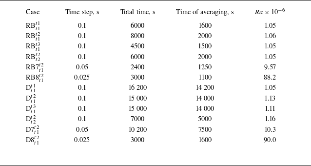
Two series of simulations have been performed, with and without an immersed disk. All cases considered are presented in table 1. The reference cases without a disk are denoted as RB (Rayleigh–Bénard) and those with a disk as D (disk). The boundary conditions used in each simulation are labelled with lower and upper indices, respectively. Thus, the label RB $_{t1}^{t3}$ means the simulation of convection in a layer without immersed disk with boundary conditions of the first type at the lower and third type at the upper boundaries.

Table 1.

Parameters of the DNS runs.

Four sets of boundary conditions for the heat transfer equation at the upper and lower boundaries are considered: fixed temperature at both boundaries X $^{t1}_{t1}$

(2.9) \begin{equation} \left .T\right |_{z=0} = T_h, \qquad \left .T\right |_{z=H} = T_c; \end{equation}

fixed temperature at the bottom and fixed heat flux at the top X $^{t2}_{t1}$

(2.10) \begin{equation} \left .T\right |_{z=0} = T_h, \qquad \left .\frac {\partial T}{\partial z}\right |_{z=H} = q_h; \end{equation}

fixed temperature at the bottom and heat exchange with the environment at the top X $^{t3}_{t1}$

(2.11) \begin{equation} \left .T\right |_{z=0} = T_h, \qquad \left .\frac {\partial T}{\partial z}\right |_{z=H} = \alpha (T_c - T_{\infty }); \end{equation}

and fixed heat flux at both boundaries X $^{t2}_{t2}$

(2.12) \begin{equation} \left .\frac {\partial T}{\partial z}\right |_{z=0} = -q_h, \qquad \left .\frac {\partial T}{\partial z}\right |_{z=H} = q_h. \end{equation}

Here, $\alpha$ is the heat transfer coefficient, $T_{\infty }$ is the environment temperature. The values of the physical characteristics at the upper boundary were chosen so as to ensure the same values of the Rayleigh number

(2.13) \begin{align} {\textit{Ra}} = g\beta H^{3}\Delta T / \nu \chi \approx 1.1 {\times}10^6, \end{align}

where $H$ is the height of the layer, $\Delta T = T_h - T_c$ is the temperature difference between the lower and upper boundaries, which is calculated as an area and time average, and $\chi$ is the thermal diffusivity. Additionally, four simulations (two without a disk and two with a disk) were performed for ${\textit{Ra}}\approx 10^7$ and ${\textit{Ra}}\approx 10^8$ . In tables 1–3 these cases are denoted as RB7 $^{t2}_{t1}$ , RB8 $^{t2}_{t1}$ and D7 $^{t2}_{t1}$ , D8 $^{t2}_{t1}$ .

Table 2.

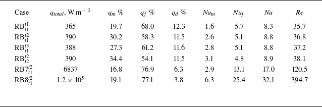
Integral characteristics of convective flows: total heat flux $q_{\textit{total}}$ and its parts, provided by mean flow ( $q_m$ ) and fluctuations ( $q_{\!f}$ ), corresponding values of Nusselt number ( $\textit{Nu}$ , ${\textit{Nu}}_m$ and ${\textit{Nu}}_{\!f}$ ), Reynolds number ${\textit{Re}}$ .

Table 3.

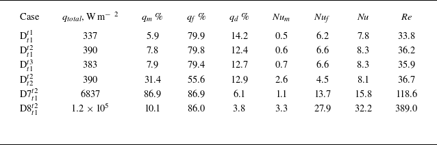
Integral characteristics of convective flows: total heat flux $q_{\textit{total}}$ and its parts, provided by mean flow ( $q_m$ ) and fluctuations ( $q_{\!f}$ ), corresponding values of Nusselt number ( $\textit{Nu}$ , ${\textit{Nu}}_m$ and ${\textit{Nu}}_{\!f}$ ), Reynolds number ${\textit{Re}}$ .

The simulations start from the resting state ( $\boldsymbol{u}=0$ ), and in cases with an immersed body, with the disk located in the centre of the layer ( $x_c = 0$ and $y_c = 0$ ). The initial temperature was set to be uniform and equal to 307 K. The physical time of simulations for each run was sufficient to achieve a statistically stationary regime, followed by averaging of at least 1000 s for the RB convection and 7000 s for the convection with the disk.

Numerical simulations were performed with the in-house Computational Fluid Dynamics (CFD) code $\sigma \textit {Flow}$ , whose numerical algorithm is based on the finite volume method for an unstructured spatial grid. The approximation of the convective and diffusion terms in the Navier–Stokes equation is carried out by the second-order central-difference schemes. The coupling between the velocity and pressure fields, which ensures the continuity equation is satisfied, is realised using a SIMPLE-like splitting procedure. The values of the velocity and pressure fields are determined at the centres of the control volumes. To eliminate oscillations of the pressure field, the Rhie–Chow approach is used, which consists of a special interpolation of the velocity vector on the faces of the control volumes. The second-order Crank–Nicolson method is used for the time integration of the equation of motion. Both the viscous and the convective terms of the equation of motion are treated implicitly. The convective terms of the energy transfer equation are approximated by a second-order upwind Total Variation Diminishing scheme, and the unsteady term of the temperature equation is approximated by a second-order three-layer scheme.

An unstructured hexagonal grid divided into two areas was used for calculations. In the area of disk motion (10 mm from the lower boundary), the grid spacing was 0.5 mm, and in the rest of the cell it was 1 mm. In total, the grid size was 6.6 million meshes. A grid convergence study was performed earlier for free-convective flow with an immersed disk in an elongated cell (Filimonov et al. Reference Filimonov, Gavrilov, Frick, Sukhanovskii and Vasiliev2025).

A mesh independence study was performed by varying the cell size of the mesh and examining the integral parameters. Verification calculations were performed for flow at the geometrical aspect ratio $\varGamma$ = 1.73, ${\textit{Ra}} = 10^7$ and $d = 0.1$ . Using the numerical solution on three different meshes with cell sizes, $h_\textit{coarse} = 0.5$ , $h_\textit{base} = 0.25$ and $h_\textit{fine} = 0.125$ mm, we performed the procedure of estimation of grid convergence and discretisation error (Celik et al. Reference Celik, Ghia, Roache and Freitas2008). The following integral parameters were chosen for the estimation: heat flux, mean kinetic energy and mean viscous dissipation rate of kinetic energy. The grid convergence index (GCI) for the fine mesh with a factor of safety of three and formal second-order accuracy does not exceed 2 %. The GCI values for the base mesh remain within 5 %. The results confirm that the numerical accuracy of the modelling with the base mesh is within acceptable limits for CFD modelling.

The accuracy of DNS depends on resolving all the flow motions ranging from the largest to the dissipative Kolmogorov scale, which is defined as $\eta = (\nu ^3/\varepsilon )^{1/4}$ , where $\varepsilon$ is the rate of turbulent energy dissipation. We performed an assessment of the Kolmogorov scale by time averaging the statistics for two flow regimes without the disk. For ${\textit{Ra}}\approx 10^7$ the cell size is less than Kolmogorov scale in the whole domain. For ${\textit{Ra}}\approx 10^8$ the ratio of the scales $\varDelta / \eta$ is less than 1.5 in the core region, and less than 2 in the near-wall region. Mesh resolution of $\varDelta / \eta \approx 2.1$ is sufficient for capturing up to third-order statistics for homogeneous isotropic turbulence (Pope Reference Pope2001). Perhaps the grid resolution near the walls is a bit coarse to obtain high-order statistics, but it is sufficient for low-order statistics.

3. Rayleigh–Bénard convection under various thermal boundary conditions

The convective cell under consideration can be referred to the case of moderate aspect ratios $\varGamma$ , since a systematic analysis of the dependence of the statistical characteristics of the velocity and temperature fluctuation fields in the convective layer has shown that various characteristics reach asymptotic values independent of the cell shape in a plane at $4\lesssim \varGamma \lesssim 32$ . So, for high Rayleigh numbers ( ${\textit{Ra}}\approx 10^9$ ) the integral quantities such as the Nusselt number and volume-averaged Reynolds number converge to the large aspect ratio limit at $\varGamma \approx 4$ , while horizontally averaged statistics such as the standard deviation and kurtosis of temperature and velocity fluctuations converge at $\varGamma \approx 8$ , the integral scale converges around $\varGamma \approx 32$ , and the more sensitive to the geometry is the peak position of the temperature variance and turbulent kinetic energy spectra, which latter only converge at $\varGamma \approx 64$ (Stevens et al. Reference Stevens, Blass, Zhu, Verzicco and Lohse2018, Reference Stevens, Hartmann, Verzicco and Lohse2024). Thus, one might expect that the integral characteristics reach the asymptote in the cell with $\varGamma =8.6$ , although the large-scale part of the velocity and temperature fields is still influenced by the lateral boundaries. It should be emphasised that, unlike most numerical studies, we consider solid adiabatic walls rather than periodic boundary conditions. Before considering the influence of a body floating in the layer, it is necessary to clarify how the convective flow structure responds to the combination of different boundary conditions at horizontal boundaries. Therefore, we begin with an analysis of convective flows in a cell of a given geometry without a floating body at ${\textit{Ra}}\approx 10^6$ and with various combinations of thermal boundary conditions at the upper and lower boundaries.

Figure 2.

Trajectories of liquid particles in the averaged velocity field for convection in the cell without the disk for ${\textit{Ra}}=10^6$ and four configurations of thermal boundary conditions: RB $^{t1}_{t1}$ (a), RB $^{t2}_{t1}$ (b), RB $^{t3}_{t1}$ (c) and RB $^{t2}_{t2}$ (d). Top view. The colour scale shows the value of velocity magnitude in mm s⁻¹.

Figure 3.

Time-averaged vertical velocity in the midheight cross-section (mm s⁻¹), for ${\textit{Ra}}=10^6$ and four configurations of thermal boundary conditions: RB $^{t1}_{t1}$ (a), RB $^{t2}_{t1}$ (b), RB $^{t3}_{t1}$ (c) and RB $^{t2}_{t2}$ (d).

Figure 4.

Time-averaged relative temperature ( $T - T_{mean}$ ) in the midheight cross-section (K), for ${\textit{Ra}}=10^6$ and four configurations of thermal boundary conditions: RB $^{t1}_{t1}$ (a), RB $^{t2}_{t1}$ (b), RB $^{t3}_{t1}$ (c) and RB $^{t2}_{t2}$ (d).

The structure of the mean convective flow in the layer under each of the four sets of boundary conditions is illustrated by figures 2–3. Figure 2 shows the trajectories of liquid particles in the averaged velocity field and figure 3 reproduces the distribution of the time-averaged vertical velocity in the midheight cross-section of the cell. Figure 4 shows the structure of the temperature field in the same horizontal cross-section.

The case with a fixed temperature at the lower and upper horizontal boundaries RB $^{t1}_{t1}$ , which is a basic case for most RB studies, is shown in panels (a) of these three figures. As expected, our results are in good agreement with those obtained for similar aspect ratios. Similar to Pandey et al. (Reference Pandey, Scheel and Schumacher2018)and Stevens et al. (Reference Stevens, Blass, Zhu, Verzicco and Lohse2018) we observe quasi-stable superstructures that are slowly changing in the horizontal plane. We can also note that similar patterns, but with periodic oscillations, were observed in RB convection in liquid metals, in the jump rope vortex regime (Akashi et al. Reference Akashi, Yanagisawa, Sakuraba, Schindler, Horn, Vogt and Eckert2022; Teimurazov et al. Reference Teimurazov, Singh, Su, Eckert, Shishkina and Vogt2023). Long-time experimental realisations have shown that the characteristic time of superstructure evolution is very large, of the order of a thousand free-fall time units (Moller et al. Reference Moller, Käufer, Pandey, Schumacher and Cierpka2022). In our simulations, superstructures are clearly visible even after averaging for 1600 s (for RB $^{t1}_{t1}$ ), which is approximately 800 free-fall times. The slow temporal evolution of the superstructures, which can be recognised against the background of short-lived small-scale structures (thermals), is shown in the corresponding movie in the Supplementary Materials.

By comparing panels (b) and (c) in figures 2 and 4, we conclude that the large-scale structure of the flow is very similar and stable in both cases, which combine the Dirichlet condition at the lower boundary with the Neumann (second-type) or Robin (third-type) condition at the upper boundary. This specific rhombic structure is probably formed due to the influence of solid boundaries because the rhombus vertices are tied to the centres of the cell side boundaries.

It is well known that, in extended horizontal liquid layers with a fixed heat flux at horizontal boundaries, a long-wave convective instability develops (Chapman & Proctor Reference Chapman and Proctor1980). This long-wave dominance determines the size of superstructures developing in the convective layer against the background of developed turbulent flow (Vieweg et al. Reference Vieweg, Scheel and Schumacher2021, Reference Vieweg, Scheel, Stepanov and Schumacher2022). The panels (d) in figures 2–4 confirm this scenario for case RB $_{t2}^{t2}$ . They show that one long-lived vortex of maximal size forms in the horizontally bounded cell, corresponding to the diagonal of the squared cell.

Figure 5.

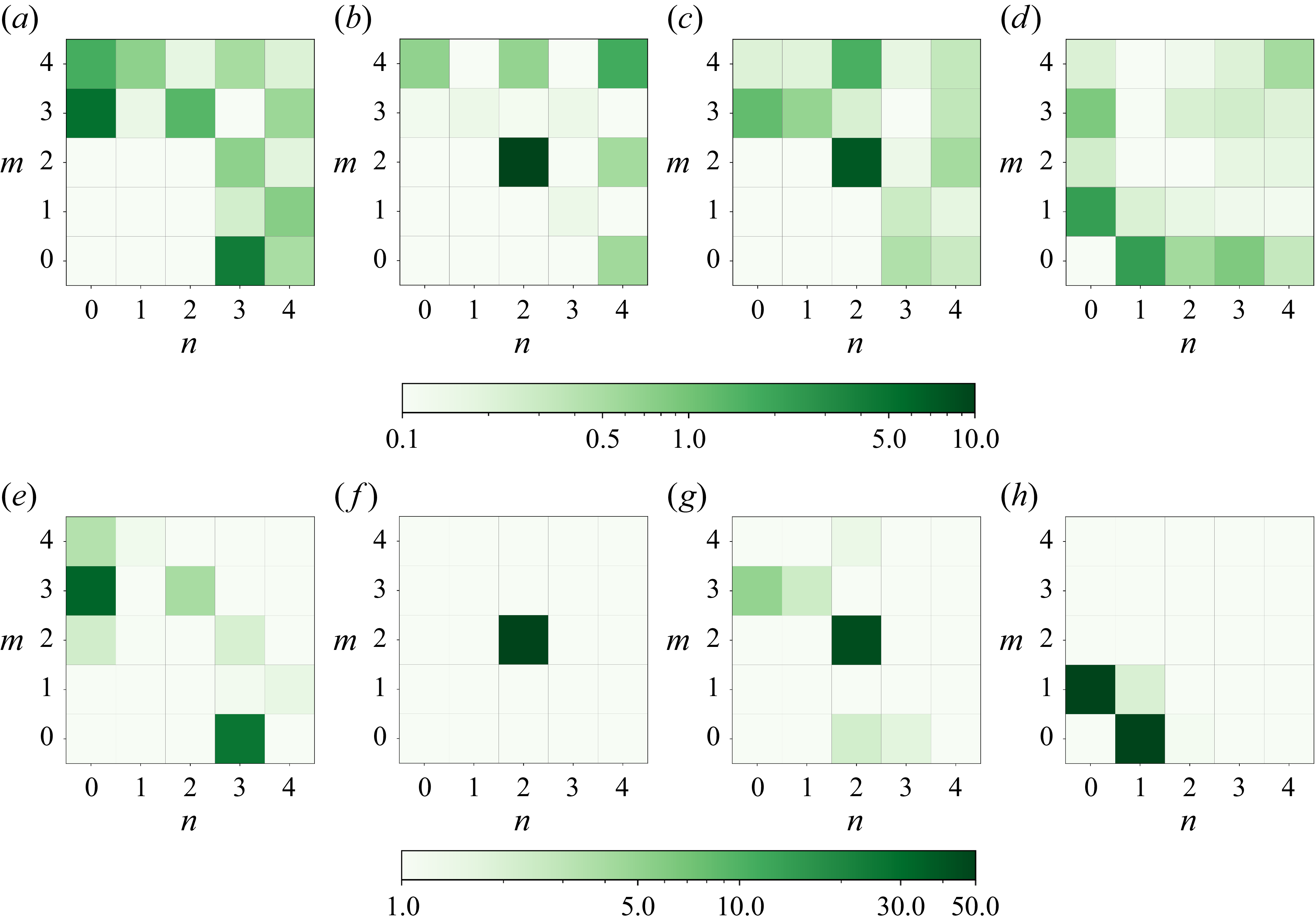
Time-averaged normalised energy (percentage) $E^{u}_{n, m}/ 0.5\langle u_{z}^{2}\rangle _{V, t}$ (upper row) and $E^{T}_{n, m}/ 0.5\langle T^{2}\rangle _{V, t}$ (lower row) of lower Fourier modes for four runs: RB $^{t1}_{t1}$ (a,e), RB $^{t2}_{t1}$ (b, f), RB $^{t3}_{t1}$ (c,g), RB $^{t2}_{t2}$ (d,h).

The formation of superstructures results in a spatially complex flow pattern. In numerical simulations with periodic vertical boundaries, the characteristic size can be determined using temperature variance spectra. In our case, the observed superstructures are relatively large. Therefore, we propose using the decomposition of horizontal two-dimensional (2-D) fields into Fourier modes to analyse the structure of large-scale flow and its time evolution

(3.1) \begin{equation} \begin{aligned} & u_{z}(\boldsymbol{r},t)=2\sum _{\boldsymbol{k}}A^{n,m}_{z}(\boldsymbol{k},t)\cos \left (k_{x}x\right )\cos(k_{y}y), \\ & T(\boldsymbol{r},t)=2\sum _{\boldsymbol{k}}A^{n,m}_{T}(\boldsymbol{k},t)\cos \left (k_{x}x\right )\cos(k_{y}y), \end{aligned} \end{equation}

where $\boldsymbol{k}=(k_{x},k_{y})$ , $k_{x}=\pi n/L$ , $k_{y}=\pi m/L$ and $n,m \in \lbrace 0,4 \rbrace$ . This approach has proven effective for analysing large-scale circulation in 2-D and 3-D RB convection (Verma Reference Verma2018; Vasiliev & Sukhanovskii Reference Vasiliev and Sukhanovskii2021; Sukhanovskii, Vasiliev & Popova Reference Sukhanovskii, Vasiliev and Popova2024).

The mean energy of each mode is evaluated as $E^{u}_{n,m}=0.5\langle (A^{n,m}_{z})^{2}\rangle _{t}$ and $E^{T}_{n,m}=0.5\langle (A^{n,m}_{T})^{2}\rangle _{t}$ , where $\langle \ldots \rangle _{t}$ denotes time averaging. The normalised and averaged energy of lower Fourier modes is shown in figure 5. The time interval used for averaging in each run is presented in table 1 and is indicated in figure 6, which shows the variation of the energy of dominating modes during the corresponding run.

Figure 5 shows noticeable differences between the number and magnitude of energy-containing modes for the vertical velocity and temperature. The temperature field has a simpler structure and is characterised by several dominant modes in all cases – the upper right corner in panels (e–h) is actually empty and in case RB $_{t1}^{t3}$ one mode (2,2) contains the most energy. This specific feature was explained by Stevens et al. (Reference Stevens, Blass, Zhu, Verzicco and Lohse2018), who showed that the kinetic energy spectra have a wide smooth maximum, while the spectra for temperature fluctuations have a sharp local maximum, demonstrating the existence of a dominant scale. This does not mean that velocity superstructures are smaller than thermal ones. A scale-by-scale analysis of the correlation between the two fields reveals that superstructures of the same size appear in both fields (Krug et al. Reference Krug, Lohse and Stevens2020). Indeed, a closer look at figure 5 shows that the main lower modes are in a perfect agreement for both fields.

Figure 6.

Time series of Fourier amplitudes $A^{n,m}_{T}$ : RB $^{t1}_{t1}$ (a), RB $^{t2}_{t1}$ (b), RB $^{t3}_{t1}$ (c), RB $^{t2}_{t2}$ (d). The grey background shows the time interval during which the averaging was done.

We considered long time intervals, which allowed us to observe significant but very slow temporal variation of the main modes (see figure 6). Time averaging is done for relatively stable time intervals for the main modes, which are shown with a grey background. The temporal behaviour and establishment of the main modes depend on the boundary conditions. In case of RB $_{t1}^{t1}$ it takes approximately 4000 s ( $\sim$ 2000 free-fall times) for stabilisation of the two dominant modes (0,3) and (3,0). For the cases RB $_{t1}^{t2}$ and RB $_{t1}^{t3}$ the dominant mode (2,2) is more stable, while the other, less energetic, modes undergo slow variations throughout the entire time interval. The described temporal variations of the energy-containing modes are not periodic, with a characteristic time of several hundred free-fall times. This is consistent with numerical and experimental estimations of the typical time required for superstructure rearrangement (Moller et al. Reference Moller, Käufer, Pandey, Schumacher and Cierpka2022). In the last case, RB $_{t2}^{t2}$ , a long transient process (also approximately 4000 s) lead to the formation of modes (0,1) and (1,0), which correspond to the large-scale diagonal vortex.

Integral characteristics of studied convective flows without the floating disk are given in table 2. The total heat flux from the bottom to the top $q_{\textit{total}}$ includes the conductive $q_{d}$ and convective $q_{conv}$ heat fluxes. The latter consists of two parts provided by the mean flow $q_{m}$ and by fluctuations $q_{\!f}$

(3.2) \begin{align}& {q_d} = \frac {1}{V}\int \limits _V {{{\left \langle { - \lambda \frac {{\partial T}}{{\partial z}}} \right \rangle }_t}{\rm d}V}=\frac {\lambda \Delta T}{H}, \end{align}

(3.3) \begin{align}&\quad {q_m} = \frac {{\rho {C_p}}}{V}\int \limits _V {{{\left \langle u_z \right \rangle }_t}{{\left \langle T \right \rangle }_t}{\rm d}V}, \end{align}

(3.4) \begin{align}&\quad\,\, {q_{\!f}} = \frac {{\rho {C_p}}}{V}\int \limits _V {{{\left \langle {u_z'T'} \right \rangle }_t}{\rm d}V}, \end{align}

where $\langle {} \rangle _t$ denotes time averaging, $\lambda$ is thermal conductivity, $u_z$ is the vertical velocity component and dashes denote the fluctuations of the corresponding quantity.

The table includes also corresponding Nusselt numbers as dimensionless characteristics of the heat flux

(3.5) \begin{equation} {\textit{Nu}} = \frac {H}{{\Delta T}}\frac {q}{\lambda }, \end{equation}

and the Reynolds number as a dimensionless characteristic of the flow intensity

(3.6) \begin{equation} {{Re}} = \frac {{H\sqrt {{{\left \langle {{\boldsymbol{u}} \boldsymbol{\cdot }{\boldsymbol{u}}} \right \rangle }_{t,V}}} }}{\nu }, \end{equation}

where $\left \langle \boldsymbol{\cdot }\right \rangle _{t,V}$ denotes averaging over the volume and time.

The values of the Nusselt and Reynolds numbers when the boundary conditions on one or both boundaries are not of the Dirichlet type are very close and approximately $6\,\%$ and $4\,\%$ larger than corresponding values in the case RB $_{t1}^{t1}$ for the same values of the Rayleigh number. This means that transition from the Dirichlet boundary condition leads to the slight decrease of the thickness of the boundary layers and slight increase of the flow circulation. A change in boundary conditions results in different ratios of the mean and fluctuating components of heat flux. This ratio is highest (approximately $3.6$ ) for RB $_{t1}^{t1}$ (constant temperature) and lowest (approximately $1.5$ ) for RB $_{t2}^{t2}$ (constant heat flux). For the mixed cases, this ratio lies between these values. This result agrees with the temporal variation of the main modes presented in figure 6. It is strongest for RB $_{t1}^{t1}$ and weakest for RB $_{t2}^{t2}$ .

4. Convection with a free–floating immersed disk

The next series of simulations were performed for the same four sets of boundary conditions and the same value of the Rayleigh number ${\textit{Ra}}=10^6$ , but for a fluid layer in which a disk is placed at a fixed height $h=4$ mm and can move in horizontal directions due to the action of viscous and pressure forces. The corresponding numerical experiments are labelled as D $^{t1}_{t1}$ , D $^{t2}_{t1}$ , D $^{t3}_{t1}$ and D $^{t3}_{t1}$ (see table 1).

Figure 7.

Trajectories of the disk centre in four runs: D $^{t1}_{t1}$ (a), D $^{t2}_{t1}$ (b), D $^{t3}_{t1}$ (c), D $^{t2}_{t2}$ (d). Only the part of the cell accessible to the movements of the disk centre is shown.

At the beginning of each run, the disk was placed in the centre of the cell. As the convective flow develops, it entrains the disk, causing it to float. The motion of the disk affects both the heat flux and the fluid flow. Figure 7 shows the trajectories of the centre of the disk in each of the four simulations. As can be seen, in the three cases, in which the temperature was fixed at the bottom of the cell and different thermal conditions were applied to the upper boundary, the disk shows complex motion, mainly along the sidewalls, with rare movements through the central part. In the case of fixed heat fluxes at both horizontal boundaries D $_{t2}^{t2}$ , the disk moves from the centre to the sidewall and then to a corner, where it remains until the end of the run.

In our simulations the disk floats near the lower boundary, preventing the ascent of hot thermals and hence reducing the heat flux. The effect of the disk on the convective flow is illustrated in figure 8, which shows a sequence of snapshots of the vertical velocity field in the midheight cross-section of the cell, taken during the time when the disk moves along the perimeter of the cell (for the case D $^{t2}_{t1}$ ). The Supplementary Materials include a movie illustrating the motion of the disk and its influence on the flow pattern.

Figure 8.

A sequence of snapshots of the vertical velocity field in the midheight cross-section of the cell for the run D $^{t2}_{t1}$ . Upper row (left to right): the disk stops in the left lower corner ( $t=$ 1143 s); the moment $t=$ 1296 s when the disk is pulling away from this corner; the disk is moving along the left side ( $t=$ 1455 s); and at $t=$ 1515 s the disk reaches the upper left corner and stops. Bottom row (right to left): the disk runs along the wall to the upper right corner $t=$ 1752 s; the disk is moving down ( $t=$ 1926 s) and reaches the lower right corner ( $t=$ 2004 s), where it stays up to $t=$ 2310 s (last snapshot). The colour scale shows the value of velocity magnitude in mm s⁻¹.

The effect of the disk on the structure of the mean convective flow is illustrated by figures 9–11, which show the particle trajectories in the averaged velocity fields (figure 9), the averaged vertical velocity (figure 10) and temperature (figure 11) distributions in the central horizontal section of the cell. Each panel in these figures should be compared with the corresponding panel of figures 2–4 showing results for convection without the disk.

Figure 9.

Trajectories of liquid particles in the averaged velocity field for convection in the cell with a floating disk for ${\textit{Ra}}=10^6$ and four configurations of thermal boundary conditions: D $^{t1}_{t1}$ (a), D $^{t2}_{t1}$ (b), D $^{t3}_{t1}$ (c) and D $^{t2}_{t2}$ (d). Top view. The colour scale shows the value of velocity magnitude in mm s⁻¹.

Figure 10.

Time-averaged vertical velocity in the midheight cross-section (mm s⁻¹), for convection with a disk at ${\textit{Ra}}=10^6$ and four configurations of thermal boundary conditions: D $^{t1}_{t1}$ (a), D $^{t2}_{t1}$ (b), D $^{t3}_{t1}$ (c) and D $^{t2}_{t2}$ (d).

Figure 11.

Time-averaged relative temperature ( $T - T_{mean}$ ) in the midheight cross-section (K), for convection with a disk at ${\textit{Ra}}=10^6$ and four configurations of thermal boundary conditions: D $^{t1}_{t1}$ (a), D $^{t2}_{t1}$ (b), D $^{t3}_{t1}$ (c) and D $^{t2}_{t2}$ (d).

First of all, the influence of the floating disk is clearly seen for the three cases with fixed temperature at the lower boundary (D $^{t1}_{t1}$ , D $^{t2}_{t1}$ and D $^{t3}_{t1}$ ). Unlike cases without a floating disk, all of these cases show a similar structure of the averaged velocity and temperature fields. The flow structure in RB $^{t2}_{t1}$ and RB $^{t3}_{t1}$ differs significantly from that of RB $^{t1}_{t1}$ with symmetric boundary conditions of the first type. It can be concluded that the active interaction of the floating disk with the lower boundary layer reduces the role of the boundary conditions at the upper boundary. The velocity and temperature fields indicate that the averaged flow is a toroidal vortex with a downward flow of cold fluid in the centre and an upward flow of hot fluid at the sidewalls. This flow structure was observed in the experiment by Frick et al. (Reference Frick, Popova, Sukhanovskii and Vasiliev2023) performed in a layer with a free upper boundary and a constant temperature at the lower boundary. These thermal boundary conditions are close to the case of D $^{t3}_{t1}$ . In general, the weak toroidal vortex causes the disk to drift toward the sidewalls, where it spends most of the time.

Similar to the case without a floating disk the constant heat flux at both boundaries (case D $^{t2}_{t2}$ ) results in a formation of stable large-scale circulation. A disk placed in the layer cannot resist the strong diagonal vortex, which pulls the disk to the corner of the cell and blocks it there. The diagonal vortex itself is transformed into two asymmetric rolls – stronger in the free corner and less strong in the corner occupied by the disk. Thus, the hot liquid flows upward in the corner with the disk and the corner diagonal to it. The cold liquid flows downward around the diagonal separating these corners, shifting towards the disk. There is pronounced upward flow around the resting disk, which forms a strong jet in the corner behind it (see figure 10 d). In addition to described differences in the structure of the mean flows, a comparison of figures 2–4 and figures 9–11 reveals that the presence of a disk results in significant differences in the average flow intensity. Specifically, there is a higher magnitude of velocity for the boundary conditions of the second type. This is a result of the blocking of the disk in the corner in the D $^{t2}_{t2}$ case. In other cases, it moves and mixes the fluid, increasing the level of velocity pulsations and decreasing the magnitude of the mean flow.

The integral characteristics of the convective flows with a disk, summarised in table 3, should be compared with those of flows without a disk (see table 2). The presence of the disk has a weak influence on both the flow intensity and integral heat transfer. The maximal decreases in the Reynolds and Nusselt numbers do not exceed 6 % and 8 %, respectively. However, the moving disk disrupts the flow and significantly changes the ratio between the heat fluxes provided by the mean flow and fluctuations – the fraction of the mean flow decreases by a factor of approximately three.

Figure 12.

Averaged vertical profiles of dimensionless temperature in the fluid layer for different cases of convection without and with an immersed disk.

Figure 12 shows the vertical profiles of dimensionless temperature in the fluid layer, defined as

(4.1) \begin{equation} \left \langle \varTheta (z) \right \rangle = \frac {{{{\left \langle T \right \rangle }_{x,y}} - {T_c}}}{{{T_h} - {T_c}}} , \end{equation}

where ${{\langle \boldsymbol{\cdot }\rangle }_{x,y}}$ denotes the averaging along the coordinates $x$ and $y$ . It can be noted that presence of the floating disk increases the mean thickness of the thermal boundary layer, due to overheating of the fluid below the disk. There is an evident decrease in mean temperature in the layer, specifically in the bulk, which is the result of heat flux inhibition near the lower boundary and a weak imbalance of heat fluxes during the transient period.

Figure 13 shows the energy distribution of the lower Fourier modes and indicates significant changes in the velocity and temperature field structures caused by the floating disk. In contrast to what was observed for convection without a disk (see figure 5), the energy distribution diagrams for convection with a disk (see figure 13) indicate a low correlation between vertical velocity and temperature. The energy distribution of the velocity field modes (top row of figure 13) shows the absence of a strong large-scale structure, which follows from the visual analysis of the velocity fields as well (see figure 14). In all cases with active disk wanderings, the temperature fields indicate the dominance of two modes, (0, 1) and (1, 0), which correspond to large-scale rolls that entrains the disk.

Figure 13.

Time-averaged normalised energy (percentage) $E^{u}_{n, m}/ 0.5\langle u_{z}^{2}\rangle _{V, t}$ (upper row) and $E^{T}_{n, m}/ 0.5\langle T^{2}\rangle _{V, t}$ (lower row) of lower Fourier modes for four runs: D $^{t1}_{t1}$ (a,e), D $^{t2}_{t1}$ (b, f), D $^{t3}_{t1}$ (c,g), D $^{t2}_{t2}$ (d,h).

Figure 14.

Instantaneous fields of vertical velocity (a,c) and temperature ( $T - T_{mean}$ ) (b,d) in the midheight cross-section of the cell for the runs RB $^{t1}_{t1}$ (upper row) and D $^{t1}_{t1}$ (lower row). The disk location is shown by a dashed line.

To better understand the distributions presented, we need to consider the temporal dynamics of individual modes presented in figure 15. We show time series of the dominant modes $A^{0,1}_{T}$ and $A^{1,0}_{T}$ for three cases with a wandering disk (D $^{t1}_{t1}$ , D $^{t2}_{t1}$ and D $^{t3}_{t1}$ ) and the time series of modes $A^{0,1}_{T}$ , $A^{1,0}_{T}$ and $A^{1,1}_{T}$ for the case D $^{t2}_{t2}$ , with a disk blocked in the corner. The latter case demonstrates a long transient process, which leads to a quite stable regime with dominant mode $A^{1,1}_{T}$ . Three other cases reveal clear quasiperiodic variations of the two main modes. Moreover, these time series show that the variations of the two modes, which characterise the temperature distribution along the axes $x$ and $y$ , are not correlated.

Figure 15.

Time series of Fourier amplitudes $A^{n,m}_{T}$ : D $^{t1}_{t1}$ (a), D $^{t2}_{t1}$ (b), D $^{t3}_{t1}$ (c), D $^{t2}_{t2}$ (d). The grey background shows the time interval during which the averaging was done.

In experiments with a disk floating in a layer with a free upper surface, it was observed that, when recording the disk position along each horizontal coordinate separately, the resulting oscillograms look like a sufficiently stable quasi-periodic process with a clearly distinguished dominant frequency (Frick et al. Reference Frick, Popova, Sukhanovskii and Vasiliev2023). We perform a similar analysis for all numerical experiments and show that, similar to the experiment, the disk motion along each coordinate appears to be quasi-periodic, with various failures and variations in the idle time of the disk at the sidewall (figure 16). The presence of a pronounced dominant frequency (period of full oscillation from one sidewall to the opposite and back) is confirmed by the power spectral densities.

Figure 16.

Disk motions along the axes $x$ (blue solid line) and $y$ (red dashed line): D $^{t1}_{t1}$ (a), D $^{t2}_{t1}$ (b), D $^{t3}_{t1}$ (c) and D $^{t2}_{t2}$ (d).

Figure 17.

Wavelet spectra of the coordinate of the centre of the disk $x_{c}(t)$ for D $^{t1}_{t1}$ (blue thick solid line), D $^{t2}_{t1}$ (green dotted line), D $^{t3}_{t1}$ (red dash-dotted line), D7 $^{t2}_{t1}$ (purple thin solid line), D8 $^{t2}_{t1}$ (brown long dashed line). The black dashed line shows the spectrum of experimental series recorded by Frick et al. (Reference Frick, Popova, Sukhanovskii and Vasiliev2023) (divided by ten).

Namely, taking into account the character of the curves, we calculate the continuous wavelet transform, defined as

(4.2) \begin{equation} W_x(\tau , t)=\tau _{-1}\int _{-\infty }^{\infty } x(t')\, \psi ^*\left (\frac {t-t'}{\tau }\right ) {\rm d}t', \end{equation}

where $\psi (t)=\exp (-t^2+\imath 2 \pi t)$ is the complex Morlet wavelet, $t$ is the time and $\tau$ is the oscillation period (for a discussion of the advantages of the wavelet technique, see e.g. Bulnes (Reference Bulnes2022)and Frick, Sokoloff & Stepanov (Reference Frick, Sokoloff and Stepanov2022)) and we show the mean (integral) wavelet spectrum

(4.3) \begin{equation} M(\tau ) = T^{-1}\int _{0}^{T} |W_x(\tau , t)|^2 {\rm d}t \end{equation}

in figure 17. Note that, in all simulations at ${\textit{Ra}}\approx 10^6$ , the main peak is almost identical, corresponding to the mean period of oscillation $\tau \approx 1380$ s, which is close to the experimental value $\tau \approx 1200$ s (Frick et al. Reference Frick, Popova, Sukhanovskii and Vasiliev2023).

Figure 18.

Time-averaged vertical velocity (a,c,e,g) and relative temperature (b,d, f,h) in the midheight cross-section, for convection without a disk (a,b,e,f) and with it (c,d, g,h) at ${\textit{Ra}}=10^7$ : RB7 $^{t2}_{t1}$ (a,b), D7 $^{t2}_{t1}$ (c,d) and ${\textit{Ra}}=10^8$ : RB8 $^{t2}_{t1}$ (e, f), D8 $^{t2}_{t1}$ (g,h).

5. Larger Rayleigh number

All the results presented above concern convective flows in the layer at Rayleigh number ${\textit{Ra}}\approx 10^6$ , which was chosen to allow comparison with the experiments of Frick et al. (Reference Frick, Popova, Sukhanovskii and Vasiliev2023), for which the range of possible Rayleigh numbers was very limited. The response of the system to changes in the Rayleigh number is a key issue in convective studies, so in the numerical experiments we increased the Rayleigh number by two orders of magnitude and considered a combination with a fixed temperature at the lower boundary and a fixed heat flux at the upper boundary at ${\textit{Ra}}\approx 10^7$ and ${\textit{Ra}}\approx 10^8$ . Simulations were performed for RB convection and convection with a disk. In tables 1–3 these cases are denoted as RB7 $^{t2}_{t1}$ , RB8 $^{t2}_{t1}$ and D7 $^{t2}_{t1}$ , D8 $^{t2}_{t1}$ . The further increase in the Rayleigh number is limited by two factors. Firstly, by reaching the limit of available computing resources and, secondly, by achieving physically realistic heating of the cell for the accepted geometry (with the considered Rayleigh number $10^8$ the dimensional temperature difference has already reached approximately 180K).

The averaged vertical velocity and relative temperature fields for the case without a floating disk for ${\textit{Ra}}\approx 10^7$ and ${\textit{Ra}}\approx 10^8$ are shown in figure 18(a,b,e, f). It is evident that the mean distributions of velocity and temperature strongly depend on the Rayleigh number. The increase from ${\textit{Ra}}=10^6$ to ${\textit{Ra}}=10^7$ leads to noticeable changes: the clear red rhombus that stood out in the vertical velocity field at ${\textit{Ra}}=10^6$ has disappeared (compare with figure 3 b). However, the characteristic size of the structures is preserved. Moreover, the blurred, rhomboidal structure is still present, but it is now blue (descending flow), i.e. the pattern has been inverted. This can be seen in the temperature field, (compare figures 18 b and 4 b), where the hot domains have changed to cold ones. The preservation of the convective flow structure is also evident in the diagrams of the energies of the lowest Fourier modes (figures 19 a,b and 5 b, f). The further increase in Rayleigh number to ${\textit{Ra}}=10^8$ is characterised by radical structure changes (figure 18 e, f) and the dominance of different Fourier modes (figure 19 e, f).

Figure 19.

Time-averaged normalised energy $E^{u}_{n, m}/ 0.5\langle u_{z}^{2}\rangle _{V, t}$ (a,c,e,g) and $E^{T}_{n, m}/ 0.5\langle T^{2}\rangle _{V, t}$ (b,d, f,h) of lower Fourier modes for ${\textit{Ra}}=10^7$ (upper row) and ${\textit{Ra}}=10^8$ (lower row): RB7 $^{t2}_{t1}$ (a,b) and D7 $^{t2}_{t1}$ (c,d), RB8 $^{t2}_{t1}$ (e, f) and D8 $^{t2}_{t1}$ (g,h).

Figure 20.

Time series of Fourier amplitudes $A^{n,m}_{T}$ : RB7 $^{t2}_{t1}$ (a), RB8 $^{t2}_{t1}$ (b), D7 $^{t2}_{t1}$ (c), D8 $^{t2}_{t1}$ (d). The grey background shows the time interval during which the averaging was done.

Unlike RB convection, the structure of the mean flow in convection with a disk does not change significantly with increasing Rayleigh number (compare figure 18 c,d,g,h with figures 10 b and 11 b). With an increase in $Ra$ , the magnitudes of velocity and temperature increase, and the hot upflows are pushed to the walls and corners. However, the energy distribution between the Fourier modes has been preserved (figure 19 c,g,h,d).

The time series of the main Fourier modes for high $Ra$ are presented in figure 20. In general, the main features of the time evolution of the main modes for convection with and without a disk are preserved. In the case of RB convection we see slow temporal evolution, while convection with a disk is characterised by stronger and faster oscillations provided by the disk’s motion.

The oscillograms for the disk motion in high $Ra$ regimes are shown in figure 21. They are qualitatively similar to the ones for ${\textit{Ra}}=10^6$ but comparison of the oscillograms reveals that the velocity of the motion of the disk increases with $Ra$ . Another particular feature is evident intermittency for ${\textit{Ra}}=10^8$ , when relatively long periods of rest near the wall are interspersed with fast jumps of the disk from one corner to another. The described growth in intermittency of the disk’s movements is illustrated in figure 22, which shows the time dependence of the magnitude of the disk’s velocity and the histograms of the distribution of the velocity magnitude at ${\textit{Ra}}\approx 10^6$ , $10^7$ and $10^8$ . As the Rayleigh number increases, the disk spends more time at rest near the wall, and the movements from one side of the wall to the other become faster (see also figure 21, where the motions along each coordinate are shown). At ${\textit{Ra}}\approx 10^6$ the disk’s standing time was 25 % of the time of the simulations, at ${\textit{Ra}}\approx 10^7$ it was 38 % and at ${\textit{Ra}}\approx 10^8$ it increased up to 63 %.

Figure 21.

Disk motions along the axes $x$ (blue solid line) and $y$ (red dashed line) at ${\textit{Ra}}\approx 10^7$ (a) and ${\textit{Ra}}\approx 10^8$ (b).

Figure 22.

Time series (a) and histograms (b) of the disk velocity magnitude for different Rayleigh numbers.

Comparing the spectra of variations of the disk’s position (figure 17) we can also conclude that the characteristic time of disk wandering decreases with increasing Rayleigh number. The main spectral peak shifts to the left and becomes wider and flatter. In fact, the dominant frequency of the disk oscillations disappears at ${\textit{Ra}} = 10^8$ . The oscillogram of the disk’s motion in figure 21 shows that the duration of the full cycle of the disk moving from one wall to the other and back varies greatly, making it difficult to even talk about an average frequency.