1. Introduction
The evolution of a passive scalar such as temperature, injected in a freely decaying homogeneous isotropic turbulent flow, is still a challenging topic. Its dynamics is governed by the velocity field and various parameters such as the Reynolds and Prandtl numbers
 $\mathit{Re}$
and
 $\mathit{Pr}={\it\nu}/{\it\kappa}$
, where
 ${\it\nu}$
is the kinematic viscosity and
 ${\it\kappa}$
the thermal diffusivity. Several publications, such as Comte-Bellot & Corrsin (Reference Comte-Bellot and Corrsin1966), Kaneda (Reference Kaneda1986), Lesieur, Montmory & Chollet (Reference Lesieur, Montmory and Chollet1987), Goto & Kida (Reference Goto and Kida1999), Lesieur (Reference Lesieur2008), have focused on theoretical analysis and numerical simulations of the passive scalar evolution and it appears that there are still open questions, such as the behaviour of the scalar field with respect to the Prandtl number or the influence of the scale at which the scalar variance is injected.
A crucial step toward the understanding of the passive scalar dynamics is the study of decay laws at very large or very small Prandtl number. First, the decay permits one to get rid of the forcing parameter and, secondly, the Comte-Bellot and Corrsin (CBC) dimensional analysis provides theoretical results concerning decay exponents of integrated quantities. Thus, for the passive scalar field, a comparison between the experimental and numerical decay exponents of integrated quantities (such as the scalar variance
 $K_{T}(t)$
, the scalar integral scale
 $L_{T}(t)$
or the scalar dissipation rate
 ${\it\epsilon}_{T}(t)$
) and the CBC theory could give interesting information on what are the main phenomena which drive the scalar decay.
Several experimental works (Lin & Lin Reference Lin and Lin1973; Warhaft & Lumley Reference Warhaft and Lumley1978; Sreenivasan et al.
Reference Sreenivasan, Tavoularis, Henry and Corrsin1980; Danaila et al.
Reference Danaila, Zhou, Anselmet and Antonia2000; Zhou et al.
Reference Zhou, Antonia, Danaila and Anselmet2000; Zhou, Antonia & Chua Reference Zhou, Antonia and Chua2002; Lee & Antonia Reference Lee and Antonia2012; Antonia et al.
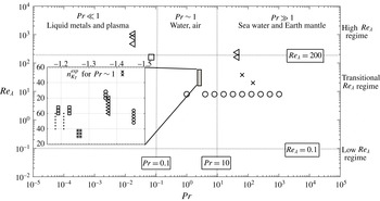
Reference Antonia, Lee, Djenidi and Danaila2013) and direct numerical simulation (DNS) (Antonia & Orlandi Reference Antonia and Orlandi2004) have already focused on scalar decay exponents. However, these scalar decay exponents exhibit a very significant dispersion, as shown in figure 1, whereas the experimental setups are designed to produce a very similar turbulent dynamics. There is up to 20 % discrepancy for similar Reynolds numbers and a fixed Prandtl number (
 $\mathit{Pr}\sim 0.7$
). This scattering between the measured scalar decay exponents may be due to transitional effects coming from the Reynolds number not being high enough, already studied in the kinetic case in Meldi & Sagaut (Reference Meldi and Sagaut2013), and also probably to the experimental turbulence production mechanisms which not permit a universal decay to be obtained. A supplementary potential explanation for the scattering might be that the flow is not fully isotropic.
Schematic view of the (
 $\mathit{Re}_{{\it\lambda}}$
,
 $\mathit{Pr}$
) combinations used for the passive scalar decay analysis. In the main figure, triangles, squares, crosses and circles respectively refer to the results of Rust & Sesonske (Reference Rust and Sesonske1966), Granatstein & Buchsbaum (Reference Granatstein and Buchsbaum1966), Yeung et al. (Reference Yeung, Xu and Sreenivasan2002) and Yeung et al. (Reference Yeung, Xu, Donzis and Sreenivasan2004). In the zoom of the small grey region at
 $\mathit{Pr}\sim 1$
, experimental scalar decay exponents of figure 10 are reported: dots, squares, stars, circles, triangles and crosses represent respectively results of Antonia et al. (Reference Antonia, Lee, Djenidi and Danaila2013), Lee & Antonia (Reference Lee and Antonia2012), Zhou et al. (Reference Zhou, Antonia, Danaila and Anselmet2000), Antonia & Orlandi (Reference Antonia and Orlandi2004) and Danaila et al. (Reference Danaila, Zhou, Anselmet and Antonia2000).

It is worth noting that the decay of a passive scalar has only been studied in experimental works and DNS in a small region of the (
 $\mathit{Re}$
,
 $\mathit{Pr}$
) map given in figure 1. In this region (the small grey zone), the Prandtl number is close to one (0.7 for air which is the most widely used fluid) and the Taylor Reynolds number (Reynolds number based on Taylor scale) is such that
 $\mathit{Re}_{{\it\lambda}}\leqslant 70$
. The values of the decay exponents obtained in these works will be reported in figure 10 along with our numerical simulations. Other experiments and DNS performed for Prandtl numbers different from one, spanning from
 $10^{-2}$
to
 $10^{2}$
in figure 1 (Granatstein & Buchsbaum Reference Granatstein and Buchsbaum1966; Rust & Sesonske Reference Rust and Sesonske1966; Yeung et al.
Reference Yeung, Xu, Donzis and Sreenivasan2004), only focus on the shape of the scalar spectrum
 $E_{T}(k,t)$
and not on the decay of the passive scalar itself. Therefore, they cannot be exploited for comparison purpose in the present study.
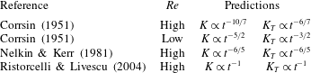
Various theoretical decay exponents for the kinetic energy and scalar variance (Corrsin Reference Corrsin1951; Nelkin & Kerr Reference Nelkin and Kerr1981; Ristorcelli & Livescu Reference Ristorcelli and Livescu2004) have been presented in table 1. The analytical study of Nelkin & Kerr is performed in the particular case of Saffman turbulence (infrared exponents of the kinetic and scalar spectra are set equal to 2): from a Richardson law, the same result as the CBC theory is derived. In Ristorcelli & Livescu, a decay law in
 $K_{(T)}\propto t^{-1}$
is derived using assumptions on statistical quantities of the flow (kinetic and scalar skewness and palinstrophy). However, this behaviour is observed in the eddy-damped quasi-normal Markovian (EDQNM) simulations only for the initial infrared exponent
 $s=1$
.
Decay exponents for the kinetic energy
 $K=\langle u_{i}u_{i}\rangle /2$
and scalar variance
 $K_{T}=\langle T\rangle /2$
at
 $\mathit{Pr}\sim 1$
.

When the Prandtl number departs from unity, as described in Tennekes & Lumley (Reference Tennekes and Lumley1972), dimensional analysis shows that at large or small Prandtl number, the shape of the scalar spectrum
 $E_{T}(k,t)$
is significantly modified at scales smaller than the integral scale. Nevertheless, as illustrated in figure 1, the regions where
 $\mathit{Pr}\ll 1$
and
 $\mathit{Pr}\gg 1$
have not been much explored for the passive scalar decay issue. Hence, an interesting question could be: does the Prandtl number, in addition to the Reynolds number and initial conditions, modify the decay laws of scalar integrated quantities
 $K_{T}(t)$
,
 $L_{T}(t)$
and
 ${\it\epsilon}_{T}(t)$
? This paper aims at answering this question, which is of interest for the understanding of passive scalar dynamics, and at providing an explanation of the scattering of experimental scalar decay exponents.
To this end, this paper focuses on two main approaches. The first one is based on the dimensional analysis of CBC, which is extended to a more general case for the passive scalar, following the work of Meldi & Sagaut (Reference Meldi and Sagaut2012) in the kinetic case. The second approach relies on the EDQNM analysis (developed by Orszag Reference Orszag1970, Reference Orszag, Balian and Peube1977, Leith Reference Leith1971 and extended to the scalar case in Herring et al.
Reference Herring, Schertzer, Lesieur, Newman, Chollet and Larcheveque1982) to perform numerical simulations of turbulent mixing. The main advantage of this method is its accuracy and low cost in investigating the turbulent dynamics for a broad range of Reynolds and Prandtl numbers. EDQNM simulations have already been used to study kinetic decay exponents (Lesieur & Ossia Reference Lesieur and Ossia2000; Meldi & Sagaut Reference Meldi and Sagaut2012, Reference Meldi and Sagaut2013) and passive scalar dynamics (Lesieur et al.
Reference Lesieur, Montmory and Chollet1987). Moreover, this method also allows one to recover theoretical results regarding the scalar spectrum shape when
 $\mathit{Pr}\leqslant 1$
and
 $\mathit{Pr}\geqslant 1$
that have been obtained in experiments and DNS (Chasnov, Canuto & Rogallo Reference Chasnov, Canuto and Rogallo1988; Lesieur & Rogallo Reference Lesieur and Rogallo1989; Antonia & Orlandi Reference Antonia and Orlandi2004; Yeung et al.
Reference Yeung, Xu, Donzis and Sreenivasan2004; Briard & Gomez Reference Briard and Gomez2015).
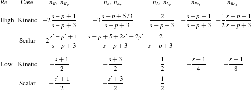
Below, new theoretical and numerical arguments are proposed to understand how the decay laws of the passive scalar field behave with a Prandtl number different from one. After describing the EDQNM modelling in § 2, the CBC theory is extended to a more general framework in § 3. Results obtained on the basis of the CBC dimensional analysis are summarized in table 2, where all the expressions using the parameters
 $s^{\prime }$
and
 $p^{\prime }$
correspond to the new scalar extension presented in this paper. Then, in §§ 4 and 5, decay exponents of scalar quantities are compared to the theoretical predictions of the CBC dimensional analysis, for both high and low Reynolds numbers. The transition between these two regimes is investigated for high and low Prandtl numbers as well. Finally, in § 6, the influence of the relative initial position of the kinetic and scalar integral scales on the dynamics is addressed. A law that can predict the relative position of the kinetic and scalar spectra peaks is derived.
Kinetic and scalar exponents for classical and extended CBC analysis.
 $K$
and
 $K_{T}$
are the kinetic energy and scalar variance,
 ${\it\epsilon}$
and
 ${\it\epsilon}_{T}$
the kinetic and scalar dissipation rates,
 $L$
and
 $L_{T}$
the kinetic and scalar integral scales,
 $\mathit{Re}_{L}$
the integral Reynolds number and
 $\mathit{Re}_{{\it\lambda}}\sim \sqrt{\mathit{Re }_{L}}$
the Reynolds number based on the Taylor microscale;
 $s$
and
 $s^{\prime }$
are the kinetic and scalar infrared slopes, and
 $p$
and
 $p^{\prime }$
backscatter parameters for the kinetic and scalar spectrum respectively. All the expressions with
 $s^{\prime }$
and
 $p^{\prime }$
are new results and will be obtained in the following sections.

2. EDQNM modelling
Isotropic homogeneous freely decaying turbulence is analysed in the present paper using the EDQNM model first introduced by Orszag (Reference Orszag1970, Reference Orszag, Balian and Peube1977) and Leith (Reference Leith1971) for hydrodynamic turbulence. In this section, a brief description of the EDQNM model is given along with the associated numerical procedure. This model is used to solve the equations of dynamics in order to obtain the time evolution of the kinetic and scalar spectra. More details about the EDQNM theory are given in appendix A and the reader is referred to Lesieur (Reference Lesieur2008) and Sagaut & Cambon (Reference Sagaut and Cambon2008) for more details.
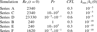
Physical and numerical parameters used for the simulations.

The EDQNM model is a quasi-normal closure. This approximation supposes that the fourth-order moments of the velocity field appearing in the evolution equation of the third-order correlations are related to the second-order moments as if the field were Gaussian. The realizability of the model is then enforced by adding an eddy-damping term
 $$\begin{eqnarray}{\it\eta}^{ED}(k,t)=a_{1}\sqrt{\int _{0}^{k}p^{2}E(p,t)\,\text{d}p}\end{eqnarray}$$
that reflects departure from Gaussianity, where
 $a_{1}=0.36$
is set to recover the Kolmogorov constant
 $K_{0}\simeq 1.40$
. The Markovianization leads to a definition of the relaxation time of the third-order moments in the EDQNM model as
 $$\begin{eqnarray}{\it\theta}_{kpq}=\frac{1-\text{e}^{-{\it\mu}_{kpq}t}}{{\it\mu}_{kpq}},\quad \text{where }{\it\mu}_{kpq}={\it\nu}(k^{2}+p^{2}+q^{2})+{\it\eta}^{ED}(k,t)+{\it\eta}^{ED}(p,t)+{\it\eta}^{ED}(q,t).\end{eqnarray}$$
Additional details concerning this closure are given in appendix A, especially regarding the scalar field.
The time evolution of the kinetic and scalar spectra
 $E(k,t)$
and
 $E_{T}(k,t)$
is obtained by solving two coupled integro-differential equations using a third-order Runge–Kutta scheme with implicit treatment of viscous terms. The wavenumber space is discretized using a logarithmic mesh
 $k_{i+1}=rk_{i}$
for
 $i=1,\ldots ,n$
, where
 $n$
is the total number of modes and
 $r=10^{1/f}$
,
 $f=17$
being the number of points per decade. This mesh spans from
 $k_{\mathit{min}}$
to
 $k_{\mathit{max}}=10k_{{\it\eta}_{T}}$
with
 $k_{{\it\eta}_{T}}=k_{B}$
if
 $\mathit{Pr}\geqslant 1$
or
 $k_{{\it\eta}_{T}}=k_{CO}$
if
 $\mathit{Pr}\leqslant 1$
. Both wavenumbers
 $k_{B}$
and
 $k_{CO}$
will be defined below. The time step
 ${\rm\Delta}t$
is monitored by setting a constant CFL number and is obtained by considering the characteristic time scales of scalar and kinetic dynamics leading to
 ${\rm\Delta}t=(\mathit{CFL}\times \mathit{Re}/20)\min \{1/k_{{\it\eta}}^{2},\mathit{Pr}/k_{{\it\eta}_{T}}^{2}\}$
. Hence the time evolution of
 ${\rm\Delta}t$
is consistent with the physical evolution of the turbulence even for very large time when the Taylor Reynolds number becomes small, i.e.
 $\mathit{Re}_{{\it\lambda}}\sim 10^{-2}$
. The values of the physical and numerical parameters are given for simulations at large and small Reynolds number in table 3.
The initial kinetic and scalar spectra
 $E$
and
 $E_{T}$
are isotropic and the shape was proposed by Pope (Reference Pope2000), Meyers & Meneveau (Reference Meyers and Meneveau2008) as
 $$\begin{eqnarray}E(k,t=0)=K_{0}k^{-5/3}{\it\epsilon}^{2/3}f_{L}(kL)f_{{\it\eta}}(k{\it\eta}),\end{eqnarray}$$
where
 $f_{L}$
and
 $f_{{\it\eta}}$
are shape functions for large and small scales, respectively:
 $$\begin{eqnarray}f_{L}(x)=\left(\frac{x}{(x^{1.5}+1.5-s/4)^{2/3}}\right)^{5/3+s},\quad f_{{\it\eta}}(x)=\exp (-5.3((x^{4}+0.4^{4})^{1/4}-0.4)).\end{eqnarray}$$
Different initial conditions were tested and there were no differences observed in the final decay regime.
3. Comte-Bellot and Corrsin dimensional analysis: scalar extension
In this section, the case
 $\mathit{Pr}=1$
is considered, for which diffusive and dissipative effects are of the same order. The influence of the Prandtl number on the decay will be discussed below in §§ 4 and 5. Here, the CBC theory (cf. Comte-Bellot & Corrsin Reference Comte-Bellot and Corrsin1966) based on a dimensional analysis, and recently extended by Meldi & Sagaut (Reference Meldi and Sagaut2012) in the purely kinetic case when the permanence of large eddies is broken, is briefly recalled. In this paper, a new correction is proposed when the infrared scalar spectrum power law exponent is
 $s^{\prime }=4$
(
 $E_{T}(k<k_{T},t)\sim k^{s^{\prime }}$
). First, the basic equations of homogeneous isotropic turbulence useful for the dimensional analysis are recalled.
3.1. Equations of homogeneous isotropic turbulence
The turbulent kinetic energy of the fluctuating velocity
 $u_{i}$
is defined as
 $K=\langle u_{i}u_{i}\rangle /2$
and the variance of temperature fluctuations
 $T$
as
 $K_{T}=\langle T^{2}\rangle /2$
, where
 $\langle \cdot \rangle$
denotes an ensemble average. Introducing the mean kinetic and scalar dissipation, respectively denoted
 ${\it\epsilon}(t)$
and
 ${\it\epsilon}_{T}(t)$
, one can write the governing equations for these global quantities
 $K(t)$
and
 $K_{T}(t)$
in a freely evolving flow as
 $$\begin{eqnarray}\frac{\text{d}K}{\text{d}t}=-{\it\epsilon}\quad \text{and}\quad \frac{\text{d}K_{T}}{\text{d}t}=-{\it\epsilon}_{T}.\end{eqnarray}$$
In turbulence, the highly diffusive flow contains a wide range of active and dynamic scales. Indeed, the velocity field fluctuations induce a rapid mixing of all the injected passive scalar. In order to characterize the dynamics of turbulent flows, several characteristic scales associated with physical mechanisms are identified. In the freely decaying isotropic case, the integral scale
 $L(t)$
carries most of the kinetic energy of the flow and can be interpreted as the characteristic size of large eddies. At Kolmogorov scale
 ${\it\eta}=({\it\nu}^{3}/{\it\epsilon})^{1/4}$
, viscous effects become dominant compared to the inertial ones, and thus
 $E(k,t)$
rapidly vanishes. The equivalent scales for the scalar field are the scalar integral scale
 $L_{T}(t)$
, the Corrsin–Obukhov scale
 ${\it\eta}_{CO}=({\it\kappa}^{3}/{\it\epsilon})^{1/4}=\mathit{Pr}^{-3/4}{\it\eta}$
, beyond which diffusion of the scalar becomes dominant, and the Batchelor scale
 ${\it\eta}_{B}=({\it\nu}{\it\kappa}^{2}/{\it\epsilon})^{1/4}=\mathit{Pr}^{-1/2}{\it\eta}$
, beyond which the scalar fluctuations are no longer agitated by small-scale convection. In spectral space, both dissipative and diffusive scales are represented respectively by the wavenumbers
 $k_{{\it\eta}}=1/{\it\eta}$
,
 $k_{CO}=1/{\it\eta}_{CO}$
and
 $k_{B}=1/{\it\eta}_{B}$
. As the scalar field dynamics is only driven by the velocity field, one can naturally use the Prandtl number
 $\mathit{Pr}={\it\nu}/{\it\kappa}$
to distinguish the three main physical regimes, i.e.
 $\mathit{Pr}\ll 1$
,
 $\mathit{Pr}=O(1)$
and
 $\mathit{Pr}\gg 1$
. The behaviour of the scalar spectrum has been derived using phenomenological arguments in Tennekes & Lumley (Reference Tennekes and Lumley1972).
Using these scales, the shape of the scalar variance spectrum
 $E_{T}$
and fluctuating kinetic energy spectrum
 $E$
can be determined by dimensional analysis. Kinetic and scalar energies and dissipation rates are linked to the spectra through
 $$\begin{eqnarray}\displaystyle & \displaystyle K(t)=\int _{0}^{\infty }E(k,t)\,\text{d}k,\quad K_{T}(t)=\int _{0}^{\infty }E_{T}(k,t)\,\text{d}k, & \displaystyle\end{eqnarray}$$
 $$\begin{eqnarray}\displaystyle & \displaystyle {\it\epsilon}(t)=2{\it\nu}\int _{0}^{\infty }k^{2}E(k,t)\,\text{d}k,\quad {\it\epsilon}_{T}(t)=2{\it\kappa}\int _{0}^{\infty }k^{2}E_{T}(k,t)\,\text{d}k. & \displaystyle\end{eqnarray}$$
Different power-law ranges for the small scales of
 $E_{T}$
have been observed in numerical simulations (Chasnov et al.
Reference Chasnov, Canuto and Rogallo1988) and also in experimental works (Grant et al.
Reference Grant, Hughes, Vogel and Moilliet1968; Sreenivasan Reference Sreenivasan1996). These power-law ranges are consistent with the abridged Lagrangian history direct interaction approximation (LHDIA) (Kraichnan Reference Kraichnan1968), direct interaction approximation (DIA) (Goto & Kida Reference Goto and Kida1999) or Lagrangian renormalized approximation (LRA) (Kaneda Reference Kaneda1986) theories. Moreover, all these ranges, present in the stationary turbulence case, can also be observed in the freely decaying turbulence framework.
3.2. Decay law for the kinetic case in the high Reynolds number regime
In the CBC theory the shape of the kinetic spectrum is taken as
 $$\begin{eqnarray}E(k)=\left\{\begin{array}{@{}ll@{}}A(t)k^{s}\quad & \text{for }k\leqslant k_{L}\text{ and }1\leqslant s\leqslant 4\\ K_{0}{\it\epsilon}^{2/3}k^{-5/3}\quad & \text{for }k_{L}\leqslant k\leqslant k_{{\it\eta}},\end{array}\right.\end{eqnarray}$$
according to the pioneering work of Kolmogorov for the inertial range. Here
 $k_{L}\simeq 1/L$
is the peak of the kinetic energy spectrum and
 $K_{0}\simeq 1.40$
is the Kolmogorov constant. The
 $k^{-5/3}$
zone is the inertial range, which goes from the wavenumber associated with the integral scale
 $k_{L}=1/L$
to the Kolmogorov wavenumber
 $k_{{\it\eta}}$
. The shape at large scales (
 $k<k_{L}$
) is referred to as the infrared range. The scaling of the kinetic energy spectrum
 $E\sim k^{s}$
is given by theoretical arguments in Batchelor & Proudman (Reference Batchelor and Proudman1956). Initial conditions with
 $s>4$
(such as a peak of energy around the integral scale) result in a large-scale spectrum in
 $k^{4}$
(Lesieur & Schertzer Reference Lesieur and Schertzer1978; Lesieur & Ossia Reference Lesieur and Ossia2000), whereas for forced turbulence, the infrared range behaves as
 $k^{2}$
(Saffman Reference Saffman1967; Lumley Reference Lumley1970). More recently, it has been shown that only the slope near the peak of energy
 $k_{L}$
(and not for
 $k\rightarrow 0$
) is important and leads the decay (Meldi & Sagaut Reference Meldi and Sagaut2012; Mons et al.
Reference Mons, Chassaing, Gomez and Sagaut2014). Finally, according to Llor & Soulard (Reference Llor and Soulard2013), it seems that any positive real values such that
 $s\leqslant 4$
could be physically acceptable.
The original method of CBC is based on the concept of invariance of very large-scale eddies corresponding to
 $k<k_{L}$
, which is notably valid for infrared slopes
 $s=1$
, 2 and 3. In fact in the kinetic case, the value of the infrared spectral slope
 $s$
is time-independent and remains constant for
 $s=1$
, 2 (Saffman), 3 and 4 (Batchelor). The coefficient
 $A(t)$
of the infrared spectrum remains constant for values of
 $s\in \{1,2,3\}$
, and evolves in time as
 $A(t)\propto L(t)^{p}$
in the case
 $s=4$
.
By dimensional analysis in the case of a high Reynolds number regime (when there is an inertial zone), one obtains
 $$\begin{eqnarray}n_{K}(s,p)=-2\frac{(s+1-p)}{(s+3-p)},\quad \text{where }K(t)\propto t^{n_{K}},\end{eqnarray}$$
in which
 $p=0$
if
 $s\leqslant 3$
and
 $p\sim 0.55$
if
 $s=4$
as computed in Lesieur et al. (Reference Lesieur, Montmory and Chollet1987), Eyink & Thomson (Reference Eyink and Thomson2000), Meldi & Sagaut (Reference Meldi and Sagaut2012). Other kinetic exponents such as
 $n_{{\it\epsilon}}$
and
 $n_{L}$
can also be determined using (3.5) and are given in table 2.
3.3. Scalar extended CBC analysis in high Reynolds and Péclet number regimes
Relevant parameters to study the dynamics of a passive scalar are not only the Reynolds number, but also the Péclet number
 $\mathit{Pe}=\mathit{Re}\,\mathit{Pr}$
. In this section, emphasis is put on the case
 $s^{\prime }=4$
. Numerical simulations show that the scalar variance also decreases with time following a power law:
 $$\begin{eqnarray}K_{T}(t)={\textstyle \frac{1}{2}}\langle T^{2}\rangle \propto t^{n_{K_{T}}}.\end{eqnarray}$$
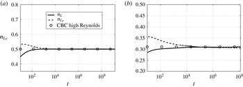
After a transient relaxation phase, the kinetic and scalar characteristic length scales exhibit the same behaviour and their decay exponents
 $n_{L}$
and
 $n_{L_{T}}$
converge toward the same value, as shown in figure 2. Consequently, we consider that
 $n_{L}=n_{L_{T}}$
, and choose as an initial condition
 $L(t=0)=L_{T}(t=0)=1$
to analyse the decay of the scalar field. It will be shown in § 6 that the relative initial position of
 $L$
and
 $L_{T}$
has no consequence for the final decay power laws, and this will justify a posteriori the present choice.
Convergence of the two scalar and kinetic characteristic length exponents
 $n_{L}$
and
 $n_{L_{T}}$
at
 $\mathit{Pr}=1$
for two cases: (a)
 $s=s^{\prime }=1$
; (b)
 $s=s^{\prime }=4$
.

At very large scales, the passive scalar field is fully controlled by the velocity one. The scalar spectrum
 $E_{T}(k,t)$
admits an asymptotic behaviour similar to
 $E(k,t)$
:
 $$\begin{eqnarray}E_{T}(k<k_{T},t)\propto k^{s^{\prime }},\quad \text{where }s^{\prime }\in [1,4],\end{eqnarray}$$
where
 $k_{T}\simeq 1/L_{T}$
is the peak of the scalar spectrum. The scalar variance spectrum depends on various physical quantities: the Prandtl number
 $\mathit{Pr}$
, the scalar dissipation
 ${\it\epsilon}_{T}$
and the kinetic energy dissipation
 ${\it\epsilon}$
. Therefore, using dimensional analysis the scalar spectrum can be written as
 $$\begin{eqnarray}E_{T}(k,t)=\left\{\begin{array}{@{}ll@{}}A_{T}(t)k^{s^{\prime }}\quad & \text{if }k\leqslant k_{T}\\ K_{CO}{\it\epsilon}_{T}{\it\epsilon}^{-1/3}k^{-5/3}\quad & \text{if }k_{T}\leqslant k\leqslant k_{{\it\eta}},\end{array}\right.\end{eqnarray}$$
where
 $K_{CO}\simeq 1.66$
is the Corrsin–Obukhov constant. In the case of a Prandtl number of order one, the scalar dynamics is exclusively dictated by the velocity field at all scales of the spectrum. This is why it exhibits a
 $k^{-5/3}$
inertial range similar to the kinetic spectrum, called the inertial–convective range, when
 $k_{T}\leqslant k\leqslant k_{{\it\eta}}$
. As mentioned in § 1, the shape of both scalar and kinetic spectra exhibits the same behaviour in terms of power-law exponents. Therefore the coefficient
 $A_{T}(t)$
varies as
 $L_{T}^{p^{\prime }}$
where
 $p^{\prime }$
only depends on
 $s$
and
 $s^{\prime }$
, as revealed in table 4.
By writing the continuity of the scalar spectrum at wavenumber
 $1/L_{T}(t)$
and considering that the passive scalar does not affect the kinetic part of the flow, one can use the expressions given in table 2:
 $n_{L}=2/(s-p+3)$
and
 $n_{{\it\epsilon}}=-3((s-p+5/3)/(s-p+3))$
, and conclude that
 $$\begin{eqnarray}{\it\epsilon}_{T}\propto t^{n_{{\it\epsilon}_{T}}},\quad \text{with }n_{{\it\epsilon}_{T}}(s,s^{\prime },p,p^{\prime })=-\frac{s-p+5+2(s^{\prime }-p^{\prime })}{s-p+3}.\end{eqnarray}$$
Moreover, as the scalar dissipation is the time derivative of scalar variance, the exponent of the scalar variance is
 $$\begin{eqnarray}n_{K_{T}}(s,s^{\prime },p,p^{\prime })=-2\frac{s^{\prime }-p^{\prime }+1}{s-p+3}.\end{eqnarray}$$
Details of the derivation of scalar exponents are very similar to those for the kinetic exponents. All corrected exponents for both kinetic and scalar cases are presented in table 2. From the theoretical decay exponents
 $n_{K}$
and
 $n_{K_{T}}$
, it seems that a decay in
 $K_{(T)}\sim t^{-1}$
(Ristorcelli Reference Ristorcelli2006) occurs only for
 $s=s^{\prime }=1$
(Meldi & Sagaut Reference Meldi and Sagaut2013) and corresponds to a constant Reynolds number.
3.4. Evaluation of
 $p^{\prime }$
with EDQNM

When setting the infrared scalar spectrum slope to
 $s^{\prime }=4$
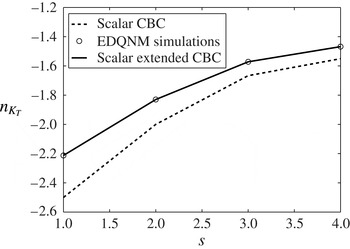
, a significant departure from the exponents obtained with the classical CBC theory and EDQNM simulations is observed. The exponent
 $n_{K_{T}}$
obtained by the classical CBC theory and EDQNM simulations is plotted in figure 3 for
 $s\in \{1,2,3,4\}$
. The observed discrepancy is essentially due to the fact that the CBC analysis of the passive scalar case assumes that the coefficient
 $A_{T}(t)$
in (3.8) is constant. But the time evolution of the scalar spectrum shows that this coefficient evolves. Therefore, the parameter
 $p^{\prime }$
cannot be considered as zero anymore for
 $s^{\prime }=4$
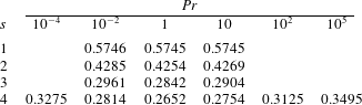
. It strongly depends on the kinetic infrared slope
 $s$
and slightly on
 $\mathit{Pr}$
(see table 4). The extended CBC analysis, also plotted in figure 3, assesses the extension proposed in the previous section.
 $n_{K_{T}}$
as function of
 $s$
obtained by EDQNM and CBC analysis when
 $s^{\prime }=4$
and
 $\mathit{Pr}=1$
.

Considering the case
 $s^{\prime }=4$
and variable infrared kinetic energy spectrum slope
 $s$
, the values of
 $p^{\prime }$
are evaluated by averaging the coefficients obtained with different exponents such as
 $n_{K_{T}}$
and
 ${\it\epsilon}_{T}$
. The estimated error in the evaluation of this parameter is around 0.25 %. Hence, the values of
 $p^{\prime }$
are computed for various Prandtl numbers and presented in table 4:
 $p^{\prime }$
decreases when
 $s$
increases at a fixed
 $\mathit{Pr}$
, and
 $p^{\prime }$
increases when
 $\mathit{Pr}$
departs from unity.
Some values of
 $p^{\prime }$
for various
 $\mathit{Pr}$
and
 $s$
with
 $s^{\prime }=4$
.

3.5. Decay laws for kinetic and scalar cases in the low Reynolds number regime
Here, emphasis is put on the dynamics of the scalar variance when considering small Reynolds numbers at
 $\mathit{Pr}=1$
. In the case of small Reynolds numbers, the inertial effects are rather small, and so inertial zone contributions to the kinetic and scalar spectra become negligible. Thus, the kinetic energy behaviour is assumed to be mainly determined by the contribution of the spectrum at large scales:
 $$\begin{eqnarray}K(t)=\int _{0}^{\infty }E(k,t)\,\text{d}k\approx \int _{0}^{k_{L}}Ck^{s}\,\text{d}k.\end{eqnarray}$$
By dimensional analysis
 $L(t)$
varies as
 $\sqrt{{\it\nu}t}$
and so
 $n_{L}=1/2$
. This leads to
 $$\begin{eqnarray}K(t)\approx \int _{0}^{k_{L}}Ck^{s}\,\text{d}k=\frac{C}{s+1}{\it\nu}^{-(s+1)/2}t^{-(s+1)/2}.\end{eqnarray}$$
Hence, from the kinetic energy
 $K$
, the dissipation rate and other important decay exponents can be deduced, all presented in table 2. One obtains the exponent of the scalar variance using the relation
 $L_{T}(t)\propto \sqrt{{\it\kappa}t}$
. Then, the integration of the scalar spectrum yields
 $$\begin{eqnarray}K_{T}(t)=\int _{0}^{\infty }E_{T}(k,t)\,\text{d}k\approx \int _{0}^{k_{T}}C_{T}k^{s^{\prime }}\,\text{d}k\end{eqnarray}$$
and
 $$\begin{eqnarray}K_{T}(t)\approx \int _{0}^{k_{T}}C_{T}k^{s^{\prime }}\,\text{d}k=\frac{C_{T}}{s^{\prime }+1}{\it\kappa}^{-(s^{\prime }+1)/2}t^{-(s^{\prime }+1)/2}.\end{eqnarray}$$
The other scalar decay exponents derived from
 $n_{K_{T}}$
are also presented in table 2. For instance,
 $n_{{\it\epsilon}_{T}}$
is simply computed using
 $(\text{d}/\text{d}t)(K_{T})={\it\epsilon}_{T}$
. In what follows, all exponents are calculated using the EDQNM simulations for both
 $s$
and
 $s^{\prime }$
in the set
 $\{1,2,3,4\}$
. For the kinetic case, there is an exact superposition of kinetic exponents with those of Lesieur & Ossia (Reference Lesieur and Ossia2000) and Meldi & Sagaut (Reference Meldi and Sagaut2012). For the scalar case, the EDQNM results for
 $s^{\prime }\leqslant 4$
are also significantly close (within 0.25 %) to the values of the CBC analysis.
4. Scalar decay at high Reynolds numbers:
$\mathit{Re}\gg 1$

The emphasis is now put on the case where the initial Reynolds number is sufficiently high to allow the kinetic and scalar spectra
 $E$
and
 $E_{T}$
to decrease according to the extended CBC exponents given in the two first lines of table 2. It will be shown in § 6 that the initial position of
 $L_{T}$
is not a governing parameter. Therefore, the initial condition
 $L(t=0)=L_{T}(t=0)$
to analyse the effect of
 $\mathit{Pr}$
on the decay exponents is relevant. This section is divided into two parts. First, the case of a very conductive passive scalar field
 $\mathit{Pr}\leqslant 1$
is investigated, and then the opposite case where convection dominates,
 $\mathit{Pr}\geqslant 1$
.
4.1. Scalar field with high diffusivity:
$\mathit{Pr}\leqslant 1$

4.1.1. General study: spectrum and decay
In this section, scalar decay exponents provided by the extended CBC theory are found to be still valid in the case where
 $\mathit{Pr}\ll 1$
(i.e.
 ${\it\nu}\ll {\it\kappa}$
). Indeed, for
 $\mathit{Pr}\sim 1$
,
 $E_{T}$
behaves like
 $E$
and all decay exponents follow the CBC extended theory whatever the values of
 $s$
and
 $s^{\prime }$
. In the case of a passive scalar with a strong diffusivity
 ${\it\kappa}$
and in the asymptotic case of high Reynolds numbers, the shape of
 $E_{T}$
is well-attested. Due to the high thermal diffusion, the temperature undergoes a rapid decrease. In this case, a more complex analysis, described by Batchelor, Howells & Townsend (Reference Batchelor, Howells and Townsend1958), is needed to obtain the scalar spectrum shape:
 $$\begin{eqnarray}E_{T}(k,t)=\frac{K_{0}}{3}{\it\epsilon}_{T}{\it\epsilon}^{2/3}{\it\kappa}^{-3}k^{-17/3}\quad \text{for }k_{CO}<k<k_{{\it\eta}}.\end{eqnarray}$$
The range
 $k\in [k_{CO};k_{{\it\eta}}]$
is the inertial–diffusive range. The
 $k^{-17/3}$
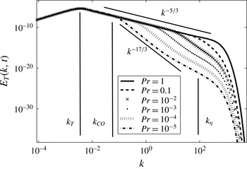
spectrum was assessed by DNS in Chasnov et al. (Reference Chasnov, Canuto and Rogallo1988), has already been observed with EDQNM in Marinis et al. (Reference Marinis, Chibbaro, Meldi and Sagaut2013), and recovered here in figure 4. There, the inertial–diffusive subrange grows in size when
 $\mathit{Pr}$
decreases. One can observe that for
 $\mathit{Pr}=10^{-5}$
there is only one decade left for the
 $k^{-5/3}$
range. The theoretical CBC exponents being based on the existence of an inertial–convective range, cases where
 $\mathit{Pr}<10^{-5}$
will not be investigated: indeed, for decreasing
 $\mathit{Pr}$
at a fixed Reynolds number, the inertial–convective range shrinks even though the kinetic spectrum still displays an inertial range. Near the Kolmogorov wavenumber
 $k_{{\it\eta}}$
, transfers slow down and thus scalar energy accumulates. This phenomenon is studied in detail in Briard & Gomez (Reference Briard and Gomez2015).
Scalar spectrum
 $E_{T}$
for
 $s=s^{\prime }=2$
, with
 $k_{L}$
and
 $k_{{\it\eta}}$
for
 $\mathit{Pr}=10^{-n}$
,
 $n\in \unicode[STIX]{x27E6}0;5\unicode[STIX]{x27E7}$
, and
 $k_{CO}$
for
 $\mathit{Pr}=10^{-5}$
. The Reynolds number is
 $\mathit{Re}_{{\it\lambda}}=5\times 10^{3}$
.

In this section, the initial Reynolds number is
 $\mathit{Re}_{{\it\lambda}}(0)=23\,330$
, high enough to ensure that
 $\mathit{Pe}=\mathit{Re}\,\mathit{Pr}\gg 1$
. As
 $E_{T}(k,t)$
is located under
 $E(k,t)$
, local energy transfers dominate. Therefore, non-local transfers
 $T_{T}^{NL}$
, defined in appendix A, are negligible. Decay exponents of
 ${\it\epsilon}_{T}$
,
 $L_{T}$
and
 $K_{T}$
are investigated in figure 5 for
 $s=s^{\prime }=2$
and
 $s=s^{\prime }=4$
. The scalar decay exponents clearly follow the extended CBC theory. The result is the same for any
 $\mathit{Pr}\leqslant 1$
once the Péclet number is large enough.
Exponents
 $n_{K_{T}}$
,
 $n_{{\it\epsilon}_{T}}$
and
 $n_{L_{T}}$
for
 $\mathit{Pr}=10^{-4}$
: (a,c,e)
 $s=s^{\prime }=2$
; (b,d,f)
 $s=s^{\prime }=4$
.

4.1.2. Remarks on large scales: backscatter and non-local transfers
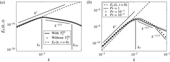
The influence of non-local transfers and Prandtl number on the infrared subrange is briefly discussed. In figure 6(a), with and without non-local transfers
 $T_{T}^{NL}$
, the scalar spectrum
 $E_{T}$
does not change, which is consistent with the previous remark: local transfers dominate. In the next section where
 $\mathit{Pr}\gg 1$
, non-local transfers strongly affect small scales.
Moreover, EDQNM simulations show that the Prandtl number does not influence the backscatter effect (
 $s=4$
or
 $s^{\prime }=4$
) for
 $\mathit{Pr}\in [10^{-5};1]$
(figure 6
b). This means that
 $\mathit{Pr}$
affects only small scales, and that the infrared slopes
 $s$
and
 $s^{\prime }$
are the sole relevant parameters at large scales.
(a) Influence of non-local transfers
 $T_{T}^{NL}$
on large scales of the scalar spectrum
 $E_{T}$
for
 $\mathit{Pr}=10^{-4}$
. (b) Influence of
 $\mathit{Pr}=1$
,
 $10^{-3}$
and
 $10^{-5}$
on backscatter.

4.2. Scalar field with low diffusivity:
$\mathit{Pr}\geqslant 1$

4.2.1. General study: spectrum and decay
In this section, the case
 $\mathit{Pr}\gg 1$
is, finally, addressed, and scalar decay exponents provided by the extended CBC theory are shown to be still valid.
In the asymptotic case of high Reynolds numbers and low diffusivity
 ${\it\kappa}$
, the scalar spectrum
 $E_{T}$
behaves as
 $k^{-1}$
at very small scales. This slope is achieved by dimensional analysis, considering that the velocity fluctuations are strongly damped by viscous effects while diffusion does not affect the temperature fluctuations. The dynamics of temperature fluctuations is then controlled by shear and friction with the characteristic time scale
 ${\it\tau}_{B}=({\it\nu}/{\it\epsilon})^{1/2}$
. In other words, beyond the Kolmogorov wavenumber, scalar fluctuations are agitated by small-scale convection of the velocity field.
Consequently, the scalar spectrum depends on
 $k$
,
 ${\it\epsilon}_{T}$
, and
 ${\it\tau}_{B}$
. Dimensional analysis leads to
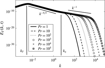
 $$\begin{eqnarray}E_{T}(k,t)=\frac{K_{0}}{3}{\it\epsilon}_{T}\sqrt{\frac{{\it\nu}}{{\it\epsilon}}}k^{-1}\quad \text{for }k_{{\it\eta}}<k<k_{B}\end{eqnarray}$$
in the so-called viscous–convective zone
 $k\in [k_{{\it\eta}};k_{B}]$
. The
 $k^{-1}$
spectrum was assessed by DNS in Yeung et al. (Reference Yeung, Xu, Donzis and Sreenivasan2004). This range is followed by a zone in which an exponential destruction of scalar fluctuations by diffusivity occurs, referred to as the viscous–diffusive range (
 $k\gg k_{B}$
).
In this section, the initial Reynolds number is
 $\mathit{Re}_{{\it\lambda}}(0)=2335$
. Unlike the previous case, non-local transfers
 $T_{T}^{NL}$
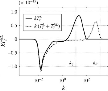
, defined in (A 23), are not negligible. Indeed, as the
 $k^{-1}$
range is located outside the kinetic spectrum
 $E$
(beyond
 $k_{{\it\eta}}$
), local energy transfers are very weak in the viscous–convective range, whereas scalar non-local transfers take energy from large scales and bring it to the very small ones (see figure 9 below). Hence, non-local transfers are dominant in the viscous–convective range. Consequently, the scalar spectrum exhibits up to a 2-decades long
 $k^{-1}$
range for a sufficiently high Prandtl number. The growth of the
 $k^{-1}$
range when
 $\mathit{Pr}$
increases is displayed in figure 7.
Scalar spectrum
 $E_{T}$
for
 $s=s^{\prime }=2$
, with
 $k_{L}$
and
 $k_{{\it\eta}}$
for
 $\mathit{Pr}=10^{n}$
,
 $n\in \unicode[STIX]{x27E6}0;5\unicode[STIX]{x27E7}$
. The Reynolds number is
 $\mathit{Re}_{{\it\lambda}}=500$
.

Finally, the decay exponents of
 ${\it\epsilon}_{T}$
,
 $L_{T}$
and
 $K_{T}$
are shown in figure 8 for
 $s=s^{\prime }=2$
and
 $s=s^{\prime }=4$
. The scalar exponents clearly follow the extended CBC theory. The result is similar for any
 $\mathit{Pr}\geqslant 1$
.
Exponents
 $n_{K_{T}}$
,
 $n_{{\it\epsilon}_{T}}$
and
 $n_{L_{T}}$
for
 $\mathit{Pr}=10^{4}$
: (a,c,e)
 $s=s^{\prime }=2$
; (b,d,f)
 $s=s^{\prime }=4$
.

4.2.2. Remarks on large scales and non-local transfers
As in the previous case,
 $\mathit{Pr}\ll 1$
, EDQNM simulations allow one to conclude that for a low diffusivity
 ${\it\kappa}$
(
 $\mathit{Pr}\gg 1$
), the Prandlt number does not affect the backscatter for
 $s=s^{\prime }=4$
; neither do the scalar non-local transfers
 $T_{T}^{NL}$
. Their impact on the total transfer (
 $\text{local}+\text{non\text{-}local}$
) is presented in figure 9 using the equality
 $$\begin{eqnarray}\int _{0}^{\infty }T_{T}^{NL}(k,t)\,\text{d}k=\int _{0}^{\infty }kT_{T}^{NL}(k,t)\,\text{d}(\log k).\end{eqnarray}$$
The non-local transfers
 $T_{T}^{NL}$
take energy from large scales and move it further than local ones, directly into the
 $k^{-1}$
viscous–convective range.
Impact of the scalar non-local transfers
 $T_{T}^{NL}$
on the total budget term
 $k\,(T_{T}+T_{T}^{NL})$
for
 $\mathit{Pr}=10^{4}$
with
 $s=s^{\prime }=4$
.

5. Transition to low Reynolds and Péclet numbers:
$\mathit{Re}\sim \mathit{Pe}\sim O(1)$

In this section, the transition from high to low Reynolds numbers with various Prandtl numbers is investigated. A detailed comparison with experimental results is performed to provide some explanations of the scattering between existing measured scalar decay exponents.
5.1. Reference case
$\mathit{Pr}=1$

5.1.1. Validation of decay exponents
The numerical method based on EDQNM analysis allows one to illustrate the transition from high to low Reynolds numbers. Several simulations are made down to very low Reynolds numbers
 $\mathit{Re}_{{\it\lambda}}\sim 10^{-1}$
, starting from
 $\mathit{Re}_{{\it\lambda}}(t=0)=236$
. This Reynolds number is high enough to capture the beginning of the transition. As will be shown, the values of all exponents obtained by EDQNM simulations are equal (within 1 % error) to their corresponding values in the CBC analysis. Hence, the scalar-extended CBC theory presented in § 3 gives a satisfactory approximation of decay exponents in the low Reynolds and Péclet number regimes.
According to the theory for the case
 $s=1$
, the same exponents for both large and small Reynolds numbers are found. It is only from the shape of the spectrum that these two cases can be distinguished. For infrared exponents
 $s\geqslant 2$
and
 $s^{\prime }\geqslant 2$
, the Reynolds number decreases over time and inertial ranges of both spectra disappear. This is the low Reynolds numbers regime and the decay exponents
 $n_{K}$
and
 $n_{K_{T}}$
converge to the values expected by the extended CBC analysis given in table 2. This transition grows more rapidly for higher values of infrared spectral slope
 $s$
and
 $s^{\prime }$
.
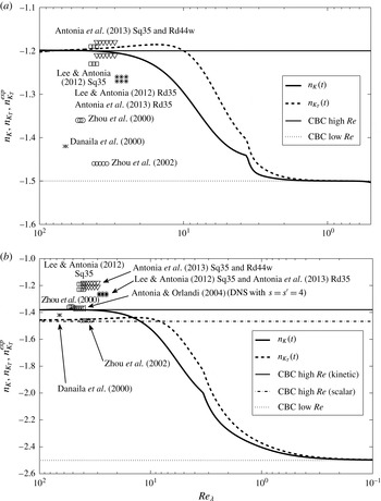
Transitions are shown for
 $s=s^{\prime }=2$
and
 $s=s^{\prime }=4$
in figure 10 along with experimental results. The case
 $s=s^{\prime }=3$
, similar to
 $s=s^{\prime }=2$
, is not presented. The small peak that appears around
 $\mathit{Re}_{{\it\lambda}}=5$
is due to the disappearance of the inertial subrange in both
 $E$
and
 $E_{T}$
. This corresponds to a transition between a regime dominated by inertial effects and a regime dominated by viscous ones. The horizontal lines correspond to theoretical predictions from the CBC theory. The experimental scalar decay exponents are displayed for both cases
 $s=s^{\prime }=2$
and
 $s=s^{\prime }=4$
.
Let us mention that, if one chooses a different initial Reynolds number, higher or lower, the resulting curve would collapse onto the present one after two turnover times
 ${\it\tau}_{0}\simeq K(0)/{\it\epsilon}(0)$
. Similarly, if different initial spectra
 $E$
and
 $E_{T}$
are prescribed, there is only a slight change during the transition. Hence, the present curves for
 $n_{K}$
and
 $n_{K_{T}}$
in the transition zone seem quite robust. Nevertheless, there is no clear power law for the decay exponent in the transition.
The critical Reynolds number at which the transition to the low Reynolds number regime begins is now briefly discussed. Two critical Reynolds numbers are observed for different kinetic and scalar cases, with infrared slope
 $s=s^{\prime }\in \{2,3,4\}$
. The critical Reynolds number for the kinetic case
 $\mathit{Re}_{{\it\lambda}}^{c}$
depends on
 $s$
, and decreases when
 $s$
increases. Transitions happen at:
-
(i) case
$s=2$
:
$\mathit{Re}_{{\it\lambda}}^{c}\approx 38$
; -
(ii) case
$s=3$
:
$\mathit{Re}_{{\it\lambda}}^{c}\approx 20$
; -
(iii) case
$s=4$
:
$\mathit{Re}_{{\it\lambda}}^{c}\approx 17$
.


The transition for the scalar field always happens around
 $\mathit{Re}_{{\it\lambda}_{T}}^{c}\approx 12$
. Other scalar exponents such as
 $n_{{\it\epsilon}_{T}}$
and
 $n_{L_{T}}$
also follow the CBC theory for low Reynolds and Péclet number regimes.
Experimental scalar decay exponents
 $n_{K_{T}}$
at
 $\mathit{Pr}\sim 1$
in comparison with high and low Reynolds number CBC theory and EDQNM simulations at
 $\mathit{Pr}=1$
. Initially,
 $L(0)=L_{T}(0)=1$
. (a)
 $s=s^{\prime }=2$
; (b)
 $s=s^{\prime }=4$
.

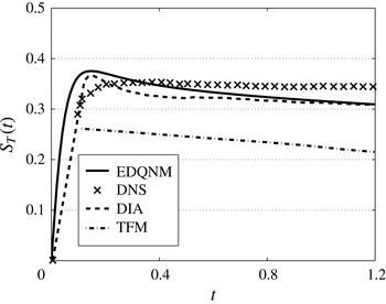
For the low Reynolds number regime itself, a validation of the EDQNM closure is proposed in appendix B where the mixed-derivative skewness
 $S_{T}$
is compared with DNS, direct-interaction approximation (DIA) and test field model (TFM) (Herring & Kerr Reference Herring and Kerr1982).
5.1.2. Review of experimental results
The aim in this section is to provide an overview of experiments for the passive scalar. In such works, the fluid is often air with
 $\mathit{Pr}\simeq 0.7$
. In figure 10, several experimental results regarding the scalar decay exponent
 $n_{K_{T}}^{exp}$
are presented in order to compare them to simulations. These values are mainly provided by Antonia & Orlandi (Reference Antonia and Orlandi2004), Lee & Antonia (Reference Lee and Antonia2012), Antonia et al. (Reference Antonia, Lee, Djenidi and Danaila2013) (DNS), Danaila et al. (Reference Danaila, Zhou, Anselmet and Antonia2000) and Zhou et al. (Reference Zhou, Antonia, Danaila and Anselmet2000, Reference Zhou, Antonia and Chua2002). One can note that experimental scalar decay exponents
 $n_{K_{T}}^{exp}$
are not close to
 $-1$
and that there is no clear tendency toward
 $-1$
with increasing Reynolds number. First, it is important to stress here that, in these experiments, the Reynolds number is rather low,
 $\mathit{Re}_{{\it\lambda}}\leqslant 70$
. EDQNM simulations show that such Reynolds numbers correspond to the beginning of the transition zone between high and low Reynolds number regimes. This could explain the broad range of scalar decay exponents that have been measured in previous years. The
 $\mathit{Re}_{{\it\lambda}}$
value is not high enough to completely match with the high Reynolds and high Péclet number regimes, and thus the
 $n_{K_{T}}^{exp}$
measured could be misrepresented by the transitional
 $\mathit{Re}_{{\it\lambda}}$
state. Even with DNS, Antonia & Orlandi (Reference Antonia and Orlandi2004) found an
 $n_{K_{T}}$
value which is not the one predicted by the CBC theory. Once again, this might be because of the low
 $\mathit{Re}_{{\it\lambda}}$
and a too low resolution of large scales (which are determinant for the decay exponents) as well. In addition to this, the infrared initial slopes
 $s$
and
 $s^{\prime }$
cannot be fixed in grid turbulence. Hence, it is impossible to compare rigorously
 $n_{K_{T}}^{exp}$
with the CBC theory.
Nevertheless, interesting results have been obtained experimentally that deserve to be emphasized. First, the scattering of the measured scalar decay exponents
 $n_{K_{T}}$
is more important than for the kinetic ones
 $n_{K}$
(Lavoie, Djenidi & Antonia Reference Lavoie, Djenidi and Antonia2007; Antonia et al.
Reference Antonia, Lee, Djenidi and Danaila2013). In addition to the two facts mentioned earlier (low
 $\mathit{Re}_{{\it\lambda}}$
and undefined infrared slopes),
 $n_{K_{T}}$
varies a lot depending on how the temperature fluctuations are generated. It has been shown (Warhaft & Lumley Reference Warhaft and Lumley1978; Sreenivasan et al.
Reference Sreenivasan, Tavoularis, Henry and Corrsin1980; Zhou et al.
Reference Zhou, Antonia, Danaila and Anselmet2000) that the measured value of
 $n_{K_{T}}$
varies significantly depending on the experimental apparatus: the power used to create the temperature fluctuations or the influence of the measurement origin (the grid, corresponding to the kinetic integral scale
 $L$
, or the heated screen, corresponding to the scalar one
 $L_{T}$
).
Recent experiments (Zhou et al.
Reference Zhou, Antonia, Danaila and Anselmet2000, Reference Zhou, Antonia and Chua2002; Lee & Antonia Reference Lee and Antonia2012; Antonia et al.
Reference Antonia, Lee, Djenidi and Danaila2013) have been performed on the scalar decay using similar parameters, which allows one to make useful comparisons. More or less all recent experiments were done with a mesh size
 $M=24.76~\text{mm}$
, an input speed
 $U\simeq 6~\text{m s}^{-1}$
, a mandoline (screen of heated wires) located at
 $x_{T}=1.5M$
and heated with 2 kW which generates temperature fluctuations
 $T\in [2~\text{K},3~\text{K}]$
. Scalar quantities are measured with the cold wires technique and the Reynolds number is
 $\mathit{Re}_{{\it\lambda}}\in [30,70]$
. However, while
 $\mathit{Re}_{{\it\lambda}}$
remains low, there is an uncertainty due to the transient phase from high Reynolds numbers to low Reynolds numbers. Finally, as the temperature is a passive scalar, it is still subjected to the variations of the kinetic field induced by the kind of grid chosen for experiments (square, round, solidity, active, passive, …). Therefore, in addition to the moderate
 $\mathit{Re}_{{\it\lambda}}$
effect, the various techniques used to create the turbulent kinetic and scalar fluctuations may be responsible for the scattering.
5.2. Case
$\mathit{Pr}\neq 1$

In the previous high Reynolds and high Péclet numbers cases, it has been shown numerically that the Prandtl number does not affect the scalar decay exponents predicted by the CBC theory. The relevant question now is to determine if this behaviour is still observed in the case of low Reynolds and low Péclet numbers. An important fact is stressed here: if the Reynolds number is low, it implies a low Péclet number regime. In other words, the case of a kinetic field in a low Reynolds number regime with a scalar field in a large Péclet regime does not exist.
5.2.1. Transition: case
$\mathit{Pr}\gg 1$

First, the case
 $\mathit{Pr}\gg 1$
is considered: for this kind of fluid, the simulations have to last longer than in the case
 $\mathit{Pr}\ll 1$
. Indeed,
 $\mathit{Re}_{{\it\lambda}}$
has to decrease a lot in order to reach the low
 $\mathit{Pe}$
regime.
The transition to a low Reynolds number regime begins when the inertial range
 $k^{-5/3}$
in the kinetic energy spectrum tends to disappear. From this point, the scalar spectrum
 $E_{T}$
still contains a
 $k^{-1}$
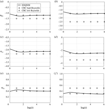
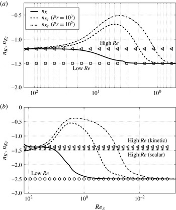
viscous–convective zone wherein the scalar destruction is fairly weak. At the beginning of the transition, with the disappearance of the inertial range, the production of small vortices stops but the friction between small scales creates some temperature fluctuations. Because of this production of temperature variance, the scalar decay slows down and the exponent of scalar variance increases. Then with the disappearance of the viscous–convective zone, the destruction of scalar variance accelerates under the cumulated effects of diffusive and dissipative processes. Hence, the scalar variance decreases with a smaller exponent. Such a behaviour is recovered in figure 11 where
 $n_{K_{T}}$
is investigated for various
 $s=s^{\prime }$
at
 $\mathit{Pr}=10^{3}$
and
 $\mathit{Pr}=10^{5}$
. The first conclusion is that scalar decay exponents provided by the extended CBC theory are still valid in the case of large Prandtl numbers. Only the behaviour of
 $n_{K_{T}}$
, before reaching its asymptotic limit, is modified by
 $\mathit{Pr}$
. Moreover, two critical Reynolds numbers are observed for the scalar field: a first one from which
 $n_{K_{T}}$
increases, and a second one from which it decreases, corresponding respectively to the disappearance of the inertial–convective and viscous–convective ranges. The second one is smaller than the one found in the case
 $\mathit{Pr}=1$
, which was
 $\mathit{Re}_{{\it\lambda}_{T}}^{c}\simeq 12$
in figure 10. Indeed, as mentioned before, reaching a low Péclet number regime with a large Prandtl number takes longer than with
 $\mathit{Pr}=1$
. Hence,
 $\mathit{Re}_{{\it\lambda}}$
has to decrease more.
Evolution of kinetic and scalar decay exponents for
 $\mathit{Re}_{{\it\lambda}}(t=0)=236$
at
 $\mathit{Pr}=10^{3}$
and
 $\mathit{Pr}=10^{5}$
: (a)
 $s=s^{\prime }=2$
; (b)
 $s=s^{\prime }=4$
.

5.2.2. Transition: case
$\mathit{Pr}\ll 1$

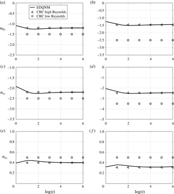
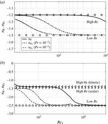
Finally, the case of a strongly diffusive fluid is studied. In figure 12, scalar decay exponents follow, once again, the extended CBC theory. There is no special behaviour of
 $n_{K_{T}}$
during the decay: indeed, all scales of the scalar spectrum
 $E_{T}$
are fully controlled by the kinetic one. In the case
 $\mathit{Pr}\ll 1$
, the main difference with respect to the case
 $\mathit{Pr}=1$
in figure 10 is that the transition happens earlier: the scalar critical Reynolds number
 $\mathit{Re}_{{\it\lambda}_{T}}^{c}(\mathit{Pr}\ll 1)$
is higher than
 $\mathit{Re}_{{\it\lambda}_{T}}^{c}(\mathit{Pr}=1)$
. As the Prandtl number is very small, the Péclet number
 $\mathit{Pe}=\mathit{Re}\,\mathit{Pr}$
tends to the low Péclet number regime faster, and so the critical Reynolds number
 $\mathit{Re}_{{\it\lambda}_{T}}^{c}$
is larger.
Evolution of kinetic and scalar decay exponents for
 $\mathit{Re}_{{\it\lambda}}(t=0)=1621$
at
 $\mathit{Pr}=10^{-3}$
and
 $\mathit{Pr}=10^{-4}$
: (a)
 $s=s^{\prime }=2$
; (b)
 $s=s^{\prime }=4$
.

It has been shown in §§ 4 and 5 that, whatever the Prandtl number is, the scalar decay exponents follow the extended CBC theory in both high and low Reynolds and Péclet number regimes. The Prandtl number does not influence the large scales of the scalar spectrum: therefore, the only relevant parameters that lead the decay of the passive scalar are the infrared slopes
 $s$
and
 $s^{\prime }$
.
6. Study of integral scales
$L$
and
$L_{T}$


In this section, emphasis is put on the evolution of the kinetic and scalar integral scales
 $L$
and
 $L_{T}$
, defined as
 $$\begin{eqnarray}L(t)=\frac{3{\rm\pi}}{4K}\int _{0}^{\infty }k^{-1}E(k,t)\,\text{d}k\end{eqnarray}$$
and
 $$\begin{eqnarray}L_{T}(t)=\frac{{\rm\pi}}{2K_{T}}\int _{0}^{\infty }k^{-1}E_{T}(k,t)\,\text{d}k.\end{eqnarray}$$
6.1. Evolution of
$L_{T}$
: Lesieur et al.’s law

The aim of this section is to show that, whatever the Prandtl number is, the relative initial position of the kinetic and scalar integral scales
 $L(t=0)$
and
 $L_{T}(t=0)$
does not change the dynamics of the decay. The law provided by Lesieur et al. (Reference Lesieur, Montmory and Chollet1987) gives the following temporal evolution of the scalar integral scale:
 $$\begin{eqnarray}L_{T}(t)=\left(\frac{n_{K}}{n_{K_{T}}}\right)^{3/2}L(t)(1+Bt^{(n_{K}-2/3)})^{3/2},\end{eqnarray}$$
where
 $B$
is a constant close to
 $-1$
evaluated from the initial conditions. The first order of this equation is
 $$\begin{eqnarray}\frac{L_{T}}{L}=\left(\frac{n_{K}}{n_{K_{T}}}\right)^{3/2}.\end{eqnarray}$$
Such an equation is obtained by dimensional analysis, assuming that in the inertial ranges,
 ${\it\epsilon}$
and
 ${\it\epsilon}_{T}$
scale as
 $$\begin{eqnarray}{\it\epsilon}=2K{\it\epsilon}^{1/3}L^{-2/3},\quad {\it\epsilon}_{T}=2K_{T}{\it\epsilon}^{1/3}L_{T}^{-2/3}.\end{eqnarray}$$
However, in the low Reynolds and low Péclet number regimes, inertial and inertial–convective ranges no longer exist. Therefore (6.3) is only valid when
 $\mathit{Re}\gg 1$
and
 $\mathit{Pe}\gg 1$
. In their paper, Lesieur et al. claim that (6.3) is only valid in the case
 $L_{T}(t=0)<L(t=0)$
, meaning that the scalar energy is injected at smaller scales than the kinetic energy.
Below, it is shown that all the three different cases,
 $L_{T}(t=0)=L(t=0)$
,
 $L_{T}(t=0)>L(t=0)$
and
 $L_{T}(t=0)<L(t=0)$
, collapse onto the same evolution after a transient phase. The cases where
 $L_{T}(t=0)=10^{2}$
and
 $10^{-2}$
, for
 $\mathit{Pr}=10^{-2}$
and
 $\mathit{Pr}=10^{2}$
with
 $L(t=0)=1$
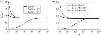
, are investigated in figure 13. Despite the large final turnover time (
 $t\sim 10^{11}$
), the Reynolds number is still high enough to ensure that there is a clear inertial range (
 $\mathit{Re}_{{\it\lambda}}\geqslant 300$
). Results before
 $t=10$
are not shown for the sake of clarity as
 $L/L_{T}$
is too high. The first conclusion is that the Prandtl number
 $\mathit{Pr}$
does not affect the time evolution of
 $L_{T}$
, as predicted by (6.3):
-
(i) if
$L_{T}(t=0)<L(t=0)$
,
$L_{T}$
catches up with the case
$L_{T}(t=0)=L(t=0)$
after a short transient state; -
(ii) if
$L_{T}(t=0)>L(t=0)$
,
$L_{T}$
catches up with the case
$L_{T}(t=0)=L(t=0)$
after a long transient state; -
(iii) this temporary state occurs whatever the Prandtl number is.






Evolution of
 $L/L_{T}$
for the three different cases
 $L_{T}(t=0)=L(t=0)$
,
 $L_{T}(t=0)>L(t=0)$
and
 $L_{T}(t=0)<L(t=0)$
: (a)
 $\mathit{Pr}=10^{-2}$
; (b)
 $\mathit{Pr}=10^{2}$
.

In conclusion, the initial position of
 $L_{T}$
is not a relevant parameter to study the decay of a passive scalar field because it does not modify its long-time dynamics. This is why, in all the previous computations, both initial temperature and velocity integral scales were assumed to be of the same order. Consequently, the initial peaks of both the kinetic and scalar spectra,
 $k_{L}$
and
 $k_{T}$
, were such that
 $k_{L}(0)=k_{T}(0)=1$
.
The result presented here is a theoretical one as
 $L$
and
 $L_{T}$
collapse onto each other for very large turnover times (at least
 $t\sim 10^{5}$
). Such large turnover times are never reached in practice in experiments. Nevertheless, the three cases
 $L(0)>L_{T}(0)$
,
 $L(0)<L_{T}(0)$
and
 $L(0)=L_{T}(0)$
are physically meaningful: the first case corresponds to an apparatus where the velocity fluctuations are heated after the grid by a mandoline for instance; the second case corresponds to a ‘toaster’, where the laminar field before the grid is heated. A comparison of these two settings has been done by Sirivat & Warhaft (Reference Sirivat and Warhaft1983). The third case corresponds to a heated grid (Warhaft & Lumley Reference Warhaft and Lumley1978).
In the high Reynolds and high Péclet number regimes, the common assumptions
 $k_{L}\simeq 1/L$
and
 $k_{T}\simeq 1/L_{T}$
are made. In the following section, a formula that allows one to predict the relative position of
 $k_{T}$
and
 $k_{L}$
is provided, valid only in the high Reynolds and Péclet number regimes.
6.2. Prediction of
$k_{L}$
and
$k_{T}$


Here, a law able to predict the relative position of the peaks of both kinetic and scalar spectra, respectively
 $k_{L}$
and
 $k_{T}$
, is derived. This law is valid in high Reynolds and Péclet number regimes, as soon as kinetic and scalar integrated quantities start to decay according to the CBC theory. We define the ratio
 $$\begin{eqnarray}{\it\beta}=\frac{k_{T}}{k_{L}}.\end{eqnarray}$$
The assumption
 ${\it\beta}=1$
is commonly made, but this value is not obtained with EDQNM simulations. Moreover, the fact that
 $k_{T}\neq k_{L}$
has already been observed in experiments: Warhaft & Lumley (Reference Warhaft and Lumley1978) and Sreenivasan et al. (Reference Sreenivasan, Tavoularis, Henry and Corrsin1980) noted that there was a link between the scalar decay exponent
 $n_{K_{T}}$
and the ratio
 $k_{T}/k_{L}={\it\beta}$
. Zhou et al. (Reference Zhou, Antonia, Danaila and Anselmet2000) also made the observation and proposed a correlation. Nevertheless, as the infrared exponents are unknown in experiments, it is impossible to make relevant comparisons. This is the reason why an analytical law linking
 ${\it\beta}$
and
 $n_{K_{T}}$
in the high Reynolds and Péclet number regimes is proposed here. For convenience, in the calculations piecewise spectra are used:
 $$\begin{eqnarray}E(k,t)=\left\{\begin{array}{@{}ll@{}}A(t)k^{s}\quad & \text{for }k<k_{L}\\ K_{0}k^{-5/3}{\it\epsilon}^{2/3}\quad & \text{for }k\in [k_{L};k_{{\it\eta}}],\end{array}\right.\end{eqnarray}$$
and
 $$\begin{eqnarray}E_{T}(k,t)=\left\{\begin{array}{@{}ll@{}}A_{T}(t)k^{s^{\prime }}\quad & \text{for }k<k_{T}\\ K_{CO}{\it\epsilon}_{T}{\it\epsilon}^{-1/3}k^{-5/3}\quad & \text{for }k_{T}<k<k_{{\it\eta}}\\ \displaystyle K_{B}{\it\epsilon}_{T}\sqrt{\frac{{\it\nu}}{{\it\epsilon}}}k^{-1}\quad & \text{for }k_{{\it\eta}}<k<k_{B}\end{array}\right.\end{eqnarray}$$
for
 $\mathit{Pr}\geqslant 1$
, and
 $$\begin{eqnarray}E_{T}(k,t)=\left\{\begin{array}{@{}ll@{}}A_{T}(t)k^{s^{\prime }}\quad & \text{for }k<k_{T}\\ K_{CO}{\it\epsilon}_{T}{\it\epsilon}^{-1/3}k^{-5/3}\quad & \text{for }k_{T}<k<k_{CO}\\ K_{B}{\it\epsilon}_{T}a^{-3}{\it\epsilon}^{2/3}k^{-17/3}\quad & \text{for }k_{CO}<k<k_{{\it\eta}}\end{array}\right.\end{eqnarray}$$
for
 $\mathit{Pr}\leqslant 1$
. The computation of the ratio
 $L/L_{T}$
yields
 $$\begin{eqnarray}\frac{L}{L_{T}}=\frac{3C^{\prime }C_{T}}{2CC_{T}^{\prime }}{\it\beta},\end{eqnarray}$$
where
 $C=(1/(1+s-p))+3/2$
,
 $C_{T}=(1/(1+s^{\prime }-p^{\prime }))+3/2$
,
 $C^{\prime }=(1/(s-p))+3/5$
and
 $C^{\prime }=(1/(s^{\prime }-p))+3/5$
. Then, using the Lesieur et al. model
 $L/L_{T}=(n_{K_{T}}/n_{K})^{3/2}$
, an explicit law for
 ${\it\beta}$
is obtained:
 $$\begin{eqnarray}{\it\beta}=\frac{2}{3}\left(\frac{s-p}{s^{\prime }-p^{\prime }}\right)\left(\frac{1+s^{\prime }-p^{\prime }}{1+s-p}\right)\left(\frac{n_{K_{T}}}{n_{K}}\right)^{3/2}.\end{eqnarray}$$
The law (6.11) is valid as soon as there are inertial and inertial–convective subranges in
 $E$
and
 $E_{T}$
, i.e. at high Reynolds and Péclet numbers. In order to show the relevance of this formula,
 ${\it\beta}$
has been computed in several cases with
 $s=s^{\prime }$
and with
 $s\neq s^{\prime }$
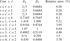
. The results are presented in table 5, where
 ${\it\beta}_{N}$
refers to the numerical results and
 ${\it\beta}_{th}$
to the theoretical ones from (6.11). This formula provides an error of less than 1 % when
 $s=s^{\prime }\leqslant 3$
and a maximum of 6.64 % when
 $s^{\prime }=4$
. Finally, the law (6.11) does not depend on the Prandtl number: all cases in table 5 give the same value for
 $\mathit{Pr}=10^{3}$
and
 $\mathit{Pr}=10^{-3}$
, consistent with the fact that
 $\mathit{Pr}$
does not affect large scales.
This law completes the work of Ristorcelli (Reference Ristorcelli2006) regarding the time scale ratio
 $r$
: in the analytical computation of
 $r$
, the ratio
 $k_{T}/k_{L}$
is introduced but no explicit formula is given.
Numerical and theoretical values of the ratio
 ${\it\beta}=k_{T}/k_{L}$
and relative error for several simulations with
 $s=s^{\prime }$
and
 $s\neq s^{\prime }$
,
 $\forall \mathit{Pr}\in [10^{-5};10^{5}]$
.

7. Conclusion
The aim of this paper is to characterize the decay of a passive scalar field in homogeneous isotropic turbulence. To this end, results from EDQNM simulations are compared to the Comte-Bellot and Corrsin (CBC) analysis, which is a simplified approach based on dimensional analysis. So far, the CBC analysis has given the exact values of the decay exponents obtained by EDQNM simulations for the infrared slopes
 $s\in \{1,2,3,4\}$
in the kinetic case. Based on the results of EDQNM simulations, an extension of the CBC analysis for passive scalar decay is presented. This corrects all scalar decay exponents of integrated quantities when the scalar infrared spectral slope
 $s^{\prime }=4$
.
The main result of this paper is that the theoretical scalar decay exponents of the extended CBC theory are valid whatever the Prandtl number is (very large, very small, and close to one) in both high and low Reynolds and Péclet number regimes. A broad range of Prandtl numbers spanning from
 $\mathit{Pr}=10^{-5}$
to
 $\mathit{Pr}=10^{5}$
was used in simulations to obtain such a general result. The main consequence of this study is that the Prandtl number only affects small scales of the scalar spectrum
 $E_{T}$
. The large scales (
 $k<k_{L}$
) depend only on the infrared slopes
 $s$
and
 $s^{\prime }$
, which is confirmed by the matching of theoretical CBC exponents and EDQNM simulations.
The impact of the relative initial position of the scalar integral scale
 $L_{T}(t=0)$
with respect to the kinetic one
 $L(t=0)$
in the case where
 $\mathit{Re}\gg 1$
and
 $\mathit{Pe}=\mathit{Re}\,\mathit{Pr}\gg 1$
is also studied. Neither the Prandtl number nor the initial position of
 $L_{T}$
affect the final result of the passive scalar decay provided that the high Reynolds and high Péclet number regimes are maintained. This result is important for a complete understanding of passive scalar decay, and shows that
 $L_{T}(t=0)$
is not a necessary parameter in long time simulations.
In other words, the problem of passive scalar decaying turbulence has been simplified, reducing the relevant parameters from (
 $\mathit{Re}$
,
 $\mathit{Pr}$
,
 $s$
,
 $s^{\prime }$
,
 $L_{T}(t=0)$
) to (
 $\mathit{Pe}$
,
 $s$
,
 $s^{\prime }$
). As a continuation of this study, a law able to predict the relative position of the peaks of both kinetic and scalar spectra
 $k_{L}$
and
 $k_{T}$
was proposed. This law, derived for the high Reynolds and high Péclet number regimes, is valid whatever the values of the Prandtl number and the infrared slopes
 $s$
and
 $s^{\prime }$
are.
In conclusion, this paper can be seen as a general study of passive scalar decay in the framework of homogeneous isotropic freely decaying turbulence. The consistency of the results over a wide range of Prandtl numbers shows that the decay of the passive scalar is driven only by the most energetic large scales of the initial spectra. Neither the initial position of the scalar integral scale nor the Prandtl number are observed to affect the final result of the decay.
Appendix A. EDQNM modelling for the kinetic and scalar fields
The spectral counterpart of the Navier–Stokes equation is written as
 $NS(k)$
:
 $$\begin{eqnarray}\frac{\partial u(k)}{\partial t}=\widehat{uu}-{\it\nu}k^{2}u(k)\end{eqnarray}$$
on the plane perpendicular to
 $k$
in order to remove the pressure term. Here,
 $u$
is the fluctuating velocity field,
 $k$
the wavenumber, and
 $\widehat{(\,)}$
the convolution product. If this equation is summed at two points
 $u(p)NS(k)$
and
 $u(k)NS(p)$
and averaged
 $\langle (\,)\rangle$
, the spectral equation of the correlation at two points is obtained:
 $$\begin{eqnarray}\left[\frac{\partial }{\partial t}+{\it\nu}(k^{2}+p^{2})\right]\langle u(k)u(p)\rangle =\langle uuu\rangle .\end{eqnarray}$$
With
 $k=p$
, the so-called Lin equation is recovered:
 $$\begin{eqnarray}\frac{\partial E(k,t)}{\partial t}+2{\it\nu}k^{2}E(k,t)=T(k,t),\end{eqnarray}$$
where
 $T(k,t)$
denotes the energy transfer between different turbulent scales. This term can be split into two types of transfers: local transfers
 $T^{L}$
representing energy exchanges between two vortices of similar size; and non-local transfers
 $T^{NL}$
representing exchanges between eddies of different size. Indeed, the kinetic energy can be transferred from one scale to another. The energy transfer of turbulent fluctuations created at a given scale to smaller ones is called the direct cascade of kinetic energy. The inverse cascade refers to the transfer occurring from small to large scales (Lesieur & Schertzer Reference Lesieur and Schertzer1978).
If the process from (A 1) to (A 2) is repeated for a three-point correlation, the following equation is obtained:
 $$\begin{eqnarray}\left[\frac{\partial }{\partial t}+{\it\nu}(k^{2}+p^{2}+q^{2})\right]\langle u(k)u(p)u(q)\rangle =\langle uuuu\rangle .\end{eqnarray}$$
One can repeat the transition from (A 2) to (A 4), but after each iteration a higher-order term appears. This is the closure problem.
In the quasi-normal approximation, the fourth-order moment of (A 4) is assumed to behave as a Gaussian random variable and can be written as the sum of the product of second-order moments:
 $$\begin{eqnarray}\left[\frac{\text{d}}{\text{d}t}+{\it\nu}(k^{2}+p^{2}+q^{2})\right]\langle u(k)u(p)u(q)\rangle =\sum \langle uu\rangle \langle uu\rangle .\end{eqnarray}$$
Orszag (Reference Orszag1970) proposed a compensation of the error due to this approximation by introducing a characteristic eddy-damping rate
 ${\it\mu}_{kpq}$
of the third-order moment associated with the triad
 $[k,p,q]$
:
 $$\begin{eqnarray}\left[\frac{\partial }{\partial t}+{\it\nu}(k^{2}+p^{2}+q^{2})+{\it\mu}_{kpq}\right]\langle u(k)u(p)u(q)\rangle =\sum \langle uu\rangle \langle uu\rangle ,\end{eqnarray}$$
with
 $$\begin{eqnarray}{\it\mu}_{kpq}={\it\nu}(k^{2}+p^{2}+q^{2})+{\it\eta}^{ED}(k,t)+{\it\eta}^{ED}(p,t)+{\it\eta}^{ED}(q,t)\end{eqnarray}$$
and
 $$\begin{eqnarray}{\it\eta}^{ED}(k,t)=a_{1}\sqrt{\int _{0}^{k}p^{2}E(p,t)\,\text{d}p},\end{eqnarray}$$
where
 $a_{1}=0.36$
so that the Kolmogorov constant
 $K_{0}=1.40$
is recovered. With this triad notation, the kinetic energy spectrum evolution equation reads
 $$\begin{eqnarray}\frac{\partial E(k,t)}{\partial t}+2{\it\nu}k^{2}E(k,t)=\int _{0}^{t}\,\text{d}{\it\tau}\int _{p+q=k}[\exp (-{\it\nu}(k^{2}+p^{2}+q^{2})(t-{\it\tau}))]\sum \langle uu\rangle \langle uu\rangle \,\text{d}p.\end{eqnarray}$$
The Markovianization consists of assuming that the exponential term in the integral does not depend on time so that integrals in (A 9) can be permuted. In addition, the characteristic time of the exponential is assumed to vary less than the one linked to
 $\sum \langle uu\rangle \langle uu\rangle$
. Therefore, the formula (A 9) can be simplified and written as
 $$\begin{eqnarray}\displaystyle & \displaystyle \frac{\partial E(k,t)}{\partial t}+2{\it\nu}k^{2}E(k,t)=\int _{p+q=k}{\it\theta}_{kpq}\sum \langle uu\rangle \langle uu\rangle (t)\,\text{d}p, & \displaystyle\end{eqnarray}$$
 $$\begin{eqnarray}\displaystyle & \displaystyle {\it\theta}_{kpq}=\int _{0}^{t}[\exp (-{\it\nu}(k^{2}+p^{2}+q^{2})(t-{\it\tau}))]\,\text{d}{\it\tau}={\it\theta}_{kpq}=\frac{1-\text{e}^{-{\it\mu}_{kpq}t}}{{\it\mu}_{kpq}}. & \displaystyle\end{eqnarray}$$
Finally the Lin equation reads
 $$\begin{eqnarray}\frac{\partial E(k,t)}{\partial t}+2{\it\nu}k^{2}E(k,t)=T^{NL}(k,t)+T^{L}(k,t),\end{eqnarray}$$
with the kinetic local transfers
 $$\begin{eqnarray}T^{L}(k,t)=\int _{{\it\Delta}_{k}}{\it\theta}_{kpq}(xy+z^{3})\frac{E(q,t)}{q}[k^{2}E(p,t)-p^{2}E(k,t)]\,\text{d}p\,\text{d}q\end{eqnarray}$$
and the non-local ones
 $$\begin{eqnarray}T^{NL}(k,t)=-\frac{\partial {\it\Pi}^{NL}}{\partial k}=-\frac{\partial ({\it\Pi}^{NL^{+}}-{\it\Pi}^{NL^{-}})}{\partial k},\end{eqnarray}$$
where
 ${\it\Pi}^{NL}$
is the non-local flux
 $$\begin{eqnarray}\displaystyle {\it\Pi}^{NL}(k,t) & = & \displaystyle \left[\frac{2}{15}k\left(E(k)-k\frac{\partial E}{\partial k}\right)\int _{0}^{ak}{\it\theta}_{kkq}q^{2}E(q)\,\text{d}q+\frac{2}{15}\frac{E(k)^{2}}{k}\int _{0}^{ak}{\it\theta}_{kkq}q^{4}\,\text{d}q\right]\nonumber\\ \displaystyle & & \displaystyle -\left[-\frac{2}{15}\int _{0}^{k}k^{\prime 2}E(k^{\prime })\,\text{d}k^{\prime }\int _{\mathit{sup}(k,k^{\prime }/a)}^{\infty }{\it\theta}_{k^{\prime }pp}\left(5E(p)+p\frac{\partial E}{\partial p}\right)\text{d}p\right.\nonumber\\ \displaystyle & & \displaystyle +\left.\frac{14}{15}\int _{0}^{k}k^{\prime 4}\,\text{d}k^{\prime }\int _{\mathit{sup}(k,k^{\prime }/a)}^{\infty }{\it\theta}_{k^{\prime }pp}\frac{E(p)^{2}}{p^{2}}\,\text{d}p\right].\end{eqnarray}$$
Due to the logarithmic discretization, the elongated triads such that
 $$\begin{eqnarray}\frac{\inf (k,p,q)}{\sup (k,p,q)}\leqslant a\end{eqnarray}$$
are not taken into account in the numerically computed energy transfers (except for isosceles interactions
 $k=p=q$
). To get rid of this difficulty a method has been developed by Lesieur & Schertzer (Reference Lesieur and Schertzer1978) and also applied to two-dimensional turbulence by Pouquet et al. (Reference Pouquet, Lesieur, Andre and Basdevant1975). In practice the non-local parameter
 $a$
is taken of
 $O(10^{-1})$
to evaluate correctly the non-local transfers due to the triadic interactions. In our simulations, the non-local parameter is
 $a=10^{1/17}-1=0.1450$
, where 17 is the number of points per decade.
The process is similar for the passive scalar. Starting from the spectral equation
 $$\begin{eqnarray}\frac{\partial T(k)}{\partial t}+{\it\kappa}k^{2}T(k)=\widehat{Tu},\end{eqnarray}$$
the characteristic third-order correlation time is
 $$\begin{eqnarray}\displaystyle & \displaystyle {\it\theta}_{kpq}^{T}=\frac{1-\exp [-({\it\kappa}(k^{2}+p^{2})+{\it\nu}q^{2}+{\it\mu}^{\prime }(k)+{\it\mu}^{\prime }(p)+{\it\mu}^{\prime \prime }(q))t]}{{\it\kappa}(k^{2}+p^{2})+{\it\nu}q^{2}+{\it\mu}^{\prime }(k)+{\it\mu}^{\prime }(p)+{\it\mu}^{\prime \prime }(q)}, & \displaystyle\end{eqnarray}$$
 $$\begin{eqnarray}\displaystyle & \displaystyle {\it\mu}^{\prime }(k)=a_{2}\sqrt{\int _{0}^{k}p^{2}E(p,t)\,\text{d}p},\quad {\it\mu}^{\prime \prime }(k)=a_{3}\sqrt{\int _{0}^{k}p^{2}E(p,t)\,\text{d}p}, & \displaystyle\end{eqnarray}$$
with
 $a_{2}=0$
and
 $a_{3}=1.3$
(see the discussion in Herring et al.
Reference Herring, Schertzer, Lesieur, Newman, Chollet and Larcheveque1982, Lesieur Reference Lesieur2008). The choice of
 $a_{2}$
and
 $a_{3}$
is based on experimental considerations so that the Corrsin constant
 $K_{CO}=0.66$
is recovered. This choice is also convenient for numerical computation. Nevertheless, a different setting (for instance
 $a_{1}=a_{2}=a_{3}$
) would lead to the same result. Finally, the so-called scalar Lin equation is obtained:
 $$\begin{eqnarray}\frac{\partial E_{T}(k,t)}{\partial t}+2{\it\kappa}k^{2}E_{T}(k,t)=T_{T}^{L}(k,t)+T_{T}^{NL}(k,t),\end{eqnarray}$$
with the scalar local transfers
 $$\begin{eqnarray}T_{T}^{L}(k)=\int _{{\it\Delta}_{k}}{\it\theta}_{kpq}^{T}\frac{k}{pq}(1-y^{2})E(q)[k^{2}E_{T}(p)-p^{2}E_{T}(k)]\,\text{d}p\,\text{d}q,\end{eqnarray}$$
and the non-local ones
 $$\begin{eqnarray}T_{T}^{NL}(k,t)=-\frac{\partial {\it\Pi}_{T}^{NL}}{\partial k}=-\frac{\partial ({\it\Pi}_{T}^{NL^{+}}-{\it\Pi}_{T}^{NL^{-}})}{\partial k},\end{eqnarray}$$
where
 ${\it\Pi}_{T}^{NL}$
is the non-local scalar flux satisfying
 $$\begin{eqnarray}\displaystyle {\it\Pi}_{T}^{NL}(k,t) & = & \displaystyle \left[k\left(2E_{T}(k)-k\frac{\partial E_{T}}{\partial k}\right)\frac{2}{15}\int _{0}^{ak}{\it\theta}_{kkq}^{T}q^{2}E(q)\,\text{d}q\right.\nonumber\\ \displaystyle & & \displaystyle +\left.\frac{1}{4}E(k)\int _{0}^{ak}{\it\theta}_{kkq}^{T}q^{3}E_{T}(q)\,\text{d}q-\frac{1}{4}\frac{E(k)E_{T}(k)}{k^{2}}\int _{0}^{ak}{\it\theta}_{kkq}^{T}q^{5}\,\text{d}q\right]\nonumber\\ \displaystyle & & \displaystyle -\left[-\frac{4}{3}\int _{0}^{k}k^{\prime 2}E_{T}(k^{\prime })\,\text{d}k^{\prime }\int _{\mathit{sup}(k,k^{\prime }/a)}^{\infty }{\it\theta}_{k^{\prime }pp}^{T}E(p)\,\text{d}p\right.\nonumber\\ \displaystyle & & \displaystyle +\left.\frac{4}{3}\int _{0}^{k}k^{\prime 4}\,\text{d}k^{\prime }\int _{\mathit{sup}(k,k^{\prime }/a)}^{\infty }{\it\theta}_{k^{\prime }pp}^{T}\frac{E(p)E_{T}(p)}{p^{2}}\,\text{d}p\right].\end{eqnarray}$$
The first term on the right-hand side of
 ${\it\Pi}_{T}^{NL}$
is responsible for the
 $k^{-1}$
viscous–convective subrange.
Appendix B. Mixed scalar skewness
$S_{T}$
in the low Reynolds number regime

An EDQNM model has already been used to study third-order statistics in homogeneous isotropic turbulence for the velocity field, for instance by Meldi & Sagaut (Reference Meldi and Sagaut2013) where the velocity skewness and palinstrophy were investigated. Here a brief validation of EDQNM closure is presented for the mixed scalar skewness
 $$\begin{eqnarray}S_{T}=\frac{\langle (\partial u/\partial x)(\partial {\it\theta}/\partial x)^{2}\rangle }{\left\langle \sqrt{(\partial u/\partial x)^{2}}\right\rangle \langle (\partial {\it\theta}/\partial x)^{2}\rangle }\end{eqnarray}$$
for low Reynolds numbers. A comparison with DNS of two-point closures has been performed in this framework by Herring & Kerr (Reference Herring and Kerr1982), where the TFM and DIA are investigated. Here, it is shown that the EDQNM model captures well the behaviour of third-order statistics.
The scalar Lin equation reads
 $$\begin{eqnarray}\left(\frac{\partial }{\partial t}+2{\it\kappa}k^{2}\right)E_{T}(k,t)=T_{T}(k,t),\end{eqnarray}$$
where
 $T_{T}$
is the total nonlinear scalar transfer. One can deduce the evolution equation of the scalar dissipation rate
 ${\it\epsilon}_{T}$
, as done by Ristorcelli (Reference Ristorcelli2006):
 $$\begin{eqnarray}\frac{\partial {\it\epsilon}_{T}}{\partial t}=-\left(\sqrt{\frac{5}{3}}S_{T}\sqrt{\mathit{Re }_{T}}+\frac{5}{9}rG_{T}\right)\frac{{\it\epsilon}{\it\epsilon}_{T}}{K}.\end{eqnarray}$$
 $S_{T}$
is the mixed scalar skewness
 $$\begin{eqnarray}S_{T}(t)=-\sqrt{\frac{3}{10}}\frac{\displaystyle \int _{0}^{\infty }k^{2}T_{T}\,\text{d}k}{\sqrt{\displaystyle \int _{0}^{\infty }k^{2}E\,\text{d}k}\displaystyle \int _{0}^{\infty }k^{2}E_{T}\,\text{d}k},\end{eqnarray}$$
 $G_{T}$
is the scalar palinstrophy
 $$\begin{eqnarray}G_{T}(t)=\frac{18}{5}{\it\kappa}\frac{K_{T}}{{\it\epsilon}_{T}}\frac{\displaystyle \int _{0}^{\infty }k^{4}E_{T}\,\text{d}k}{\displaystyle \int _{0}^{\infty }k^{2}E_{T}\,\text{d}k},\end{eqnarray}$$
 $\mathit{Re}_{T}$
is the turbulent Reynolds number
 $\mathit{Re}_{T}=K^{2}/({\it\nu}{\it\epsilon})$
, and
 $r$
is the time-scale ratio
 $(K{\it\epsilon}_{T})/(K_{T}{\it\epsilon})$
.
Comparison of the mixed scalar skewness computed with the EDQNM model with DNS, DIA and TFM of Herring & Kerr (Reference Herring and Kerr1982).

Figure 2 of Herring and Kerr shows that
 $\mathit{Re}_{{\it\lambda}}$
decreases from 12 to 6 with initial Batchelor
 $k^{4}$
spectrum. In figure 14 here,
 $S_{T}$
computed with the EDQNM model is displayed. The same initial conditions as in Herring and Kerr have been used. The final value obtained with the EDQNM model is in good agreement with DIA, close to DNS, and does not present the same problem as TFM, which slightly underestimates
 $S_{T}$
for low Reynolds numbers. The initial growth phase is well-captured with regard to DNS as well.