





1. Introduction
Moving fluid through a conduit requires energy to overcome the friction between the fluid and the bounding walls. A pumping device provides this energy, which dissipates in stationary flows. Many investigations have focused on reducing energy costs by rearranging fluid motion to minimize friction – this is the primary objective of flow control research, where the goal is to reach conditions in which the energy saved through drag reduction exceeds the energy cost of control (Ricco, Skote & Leschnizer Reference Ricco, Skote and Leschnizer2021). This direction was pursued primarily through the analysis of the effect of flow modulations created by wall transpiration (Min et al. Reference Novak and Floryan2006; Mamori, Iwamoto & Murata Reference Novak and Floryan2014; Gomez et al. Reference Novak and Floryan2016; Han & Huang Reference Novak and Floryan2020; Jiao & Floryan Reference Novak and Floryan2021a , Reference Novak and Floryanb ), even attaining sustained sublaminar levels of drag (Min et al. Reference Novak and Floryan2006; Jiao & Floryan Reference Novak and Floryan2021a , Reference Novak and Floryanb ). Bewley (Reference Floryan, Haq and Panday2009) and Fukagata, Sugiyama & Kasagi (Reference Novak and Floryan2009) proved that net energy reduction could not be achieved. Recent results indicate that combining different forms of modulation, such as adding in-plane wall oscillations, can lead to net energy savings (Floryan Reference Floryan2023).
The amount of fluid being moved depends on the available pumping power, and the properties of pumping devices limit the power they can deliver. This leads to a search for alternative propulsion systems, where energy is invested in reducing friction rather than overpowering it. Such methods enable higher flow rates at the same pumping power. The success of this concept is measured by increased flow rate rather than net energy savings, offering an alternative perspective on flow control.
Fluid heating generates a buoyancy force that acts in the opposite direction to gravity. This force has been widely used in venting combustion gases from fireplaces and is known as the chimney effect (Putnam Reference Putnam1882). This effect occurs in conduits with an orientation that provides a buoyancy force component parallel to the conduit axis – heated fluid inside the chimney is lighter than the fluid outside, creating a pressure gradient that pumps the fluid upwards passively. The conduit vertical placement is most effective, with chimney-effect strength decreasing as the conduit inclination increases away from vertical and disappearing altogether in horizontal conduits. This effect has been used for passive cooling (Naylor, Floryan & Tarasuk Reference Novak and Floryan1991; Straatman et al. Reference Straatman, Tarasuk and Floryan1993, Reference Straatman, Tarasuk and Floryan1994; Novak & Floryan Reference Novak and Floryan1995; Shahin & Floryan Reference Shahin and Floryan1999) and passive ventilation (Linden Reference Novak and Floryan1999; Tournier, Gethon & Rabinowicz Reference Tournier, Gethon and Rabinowicz2000; Wong & Heryanto Reference Wong and Heryanto2004; Andreozzi, Buonomo & Manca Reference Floryan, Haq and Panday2005; Weil Reference Weil2012; Song et al. Reference Song, Huang, Kuenzer, Zhu, Jiang, Pan and Zhong2020; Nagler Reference Novak and Floryan2021).
An effect similar to the chimney effect can be created in horizontal slots through a pattern interaction effect, which requires a proper combination of heating and topography patterns (Abtahi & Floryan Reference Floryan, Haq and Panday2017; Inasawa, Hara & Floryan Reference Inasawa, Hara and Floryan2021; Floryan & Inasawa Reference Novak and Floryan2021). The heating pattern creates a pattern of convection rolls, which induce a pattern of pressure in the slot. The pressure field projects onto the groove pattern, creating a net horizontal pressure force at the grooved wall that drives the fluid in the horizontal direction in the absence of a mean horizontal pressure gradient (Abtahi & Floryan Reference Floryan, Haq and Panday2017). The position of the heating pattern dictates the position of the pressure field, so varying the position of the heating pattern leads to different projections of the pressure field on the grooved wall, producing net flow either to the left or to the right, or no net flow at all. Results reported by Abtahi & Floryan (Reference Floryan, Haq and Panday2017) are limited to small groove amplitude (
 $A\lt 0.16$
in the notation used in this paper; see figure 1 for the definition of
 $A$
), demonstrating the efficacy of using pattern interaction for pumping (Floryan et al. Reference Floryan, Haq and Panday2022a
) and providing a basis for the development of passive ventilation systems. The flow rate driven by the pattern interaction effect increases linearly with increasing groove amplitude (Abtahi & Floryan Reference Floryan, Haq and Panday2017). It must decrease to zero as the groove tips approach the opposite wall, where the flow would be choked. Therefore, there must be a groove amplitude that maximizes the flow rate. This investigation aims to determine the groove geometry and the relative position of topography and temperature patterns required to achieve the maximum flow rate, providing the basis for estimating the viability and capabilities of passive ventilation systems based on the principle of pattern interaction.
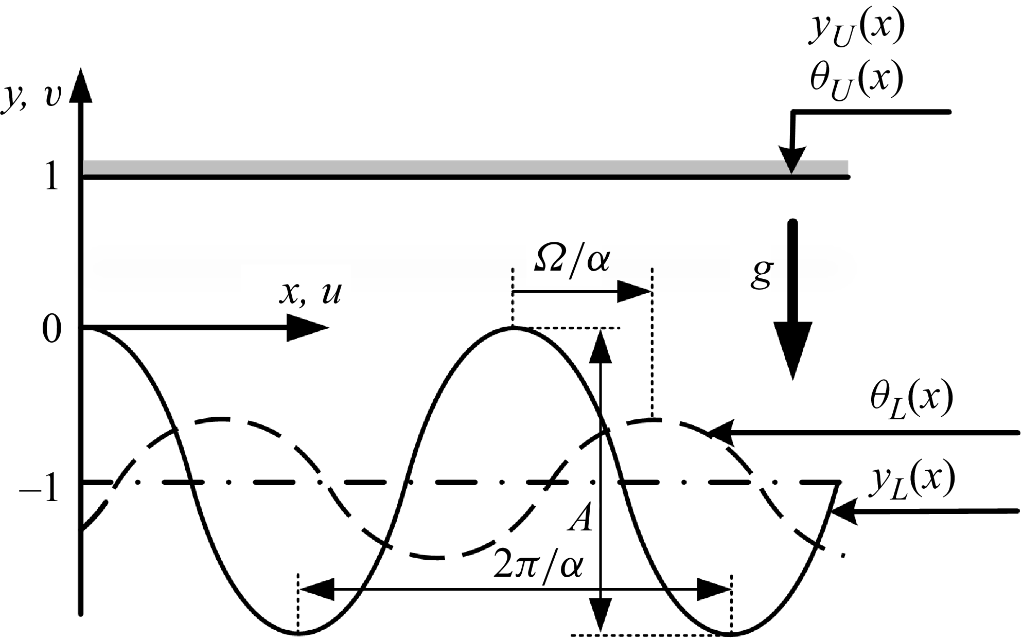
A schematic of the flow system. The lower plate temperature is given by (2.2a
). The groove and heating patterns are characterized by the wavenumber
 $\alpha$
with
 $\varOmega$
describing their relative position.

The fluid pumping created by the pattern interaction effect can be used to reduce flow losses in conduits. The heating in the case of a smooth conduit generates three effects: (i) a system of rolls that reduces the direct contact between the stream and the bounding walls; (ii) adds propulsion as buoyancy gradients drive fluid rotation within the rolls; (iii) reduces the flow cross-sectional area. The pressure losses are reduced as long as the rolls remain in the flow (Hossain, Floryan & Floryan Reference Novak and Floryan2012; Floryan & Floryan Reference Floryan, Haq and Panday2015; Hossain & Floryan Reference Hossain and Floryan2016; Inasawa, Taneda & Floryan Reference Novak and Floryan2019). An excessively fast stream washes these rolls away, which limits this technique to applications in flows with the Reynolds number
 $\textit{Re}={U_{\textit{max}}h}/{\nu }\lt 100$
where
 $h$
stands for the half-channel height,
 $U_{\textit{max}}$
stands for the maximum velocity of unmodified flow and
 $\nu$
represents the kinematic viscosity. The addition of grooves activates pumping driven by the pattern interaction effect. Proper positioning of both patterns can lead to a substantial reduction in flow losses, even self-pumping or a substantial increase in flow losses (Floryan, Shadman & Hossain Reference Floryan, Shadman and Hossain2018; Hossain & Floryan Reference Hossain and Floryan2020; Floryan et al. Reference Floryan, Wang and Bassom2024a
,
Reference Floryan, Shadman and Hossainc
). Similar effects occur in inclined slots, but the system response is more complex due to a combination of the pattern interaction effect with the component of buoyancy force acting along the conduit axis (Floryan et al. Reference Novak and Floryan2022b
,
Reference Novak and Floryanc
, Reference Floryan, Wang and Bassom2023a
, Reference Floryan, Wang and Bassom2024b
). It is worth mentioning the use of thermal waves for pumping and reducing flow losses, as such waves can be viewed as moving heating patterns (Hossain & Floryan 2023, 2024).
This presentation begins with § 2, providing a brief description of the model problem used to demonstrate pumping effectiveness and the numerical methods employed to solve the model equations. Section 3 discusses the system performance achieved with heated grooves placed on a single plate. Section 4 discusses heated grooves on both plates, divided into three parts. Section 4.1 describes grooves placed in a manner that form a wavy slot; § 4.2 deals with grooves placed in a manner leading to a converging–diverging slot; § 4.3 considers a configuration that is halfway between the converging–diverging and wavy slots. A summary of the main results is provided in § 5.
2. Problem formulation
We demonstrate the pumping capabilities of the pattern interaction effect by considering a simple model problem introduced by Abtahi & Floryan (Reference Floryan, Haq and Panday2017), which preserves all essential physics. The following presentation provides a brief outline. The model consists of an infinite horizontal slot formed by parallel plates, with the lower plate equipped with grooves, as illustrated in figure 1. The x-axis is horizontal, and the y-axis is upward. The resulting slot geometry has the form
 \begin{equation}y_{L}(x)=-1+\frac{1}{2}A\cos \alpha x,\quad y_{U}(x)=1,\end{equation}
where the subscripts L and U refer to the lower and upper plates, respectively, and the half-mean slot opening h is used as the length scale. The grooves have peak-to-trough amplitudes
 $A,$
and their pattern is characterized by the wavenumber
 $\alpha$
(or of wavelength
 $\lambda =2\pi /\alpha )$
.
The upper plate is isothermal, and the lower plate is periodically heated. The upper and lower temperature distributions are given by
 \begin{equation}\theta _{L}(x)={\textit{Ra}_{\textit{uni}}}+\frac{1}{2}\textit{Ra}_{\!p}\cos \left(\alpha x+\varOmega \right) \quad \text{and} \quad\theta _{U}(x)=0,\end{equation}
where
 $\theta$
denotes the dimensionless temperature field defined to be
 $\theta =T-T_{U}$
, and the temperature of the upper plate
 $T_{U}$
is used as a reference. Here
 $\theta$
has been scaled on
 $\kappa \nu /(g\varGamma h^{3})$
, where g is the gravitational acceleration,
 $\varGamma$
denotes the thermal expansion coefficient,
 $\nu$
is the kinematic viscosity and
 $\kappa$
is the thermal diffusivity. The periodic Rayleigh number
 $\textit{Ra}_{\!p}$
and the uniform Rayleigh number
 $\textit{Ra}_{\textit{uni}}$
measure the amplitude of periodic temperature variations and the intensity of the uniform heating, respectively.
We wish to examine the horizontal flow rate
 $Q$
induced by the interaction of heating and topography patterns (see (2.6) for its definition). To address this issue, we solve for the two-dimensional convection of Boussinesq fluid within the slot, which is governed by the continuity, Navier–Stokes and energy equations, which we write in the form
 \begin{equation}\frac{\partial u}{\partial x}+\frac{\partial v}{\partial y}=0,\quad u\frac{\partial u}{\partial x}+v\frac{\partial u}{\partial y}=-\frac{\partial p}{\partial x}+\boldsymbol{\nabla} ^{2}u,\end{equation}
 \begin{equation}u\frac{\partial v}{\partial x}+v\frac{\partial v}{\partial y}=-\frac{\partial p}{\partial y}+\boldsymbol{\nabla} ^{2}v+\textit{Pr}^{-1}\theta,\quad u\frac{\partial \theta }{\partial x}+v\frac{\partial \theta }{\partial y}=\textit{Pr}^{-1}\boldsymbol{\nabla} ^{2}\theta.\end{equation}
In the above, (
 $u$
,
 $v$
) denotes the velocity components in the (x, y) directions, respectively, scaled with
 $U_{v}=\nu /h$
while
 $p$
is the pressure relative to the hydrostatic component and scaled on
 ${\rho U}_{\nu }^{2}$
where
 $\rho$
stands for fluid density. The parameter
 $\textit{Pr}=\nu /\kappa$
is the Prandtl number, and computations reported in the paper have been carried out with Pr = 0.73 (the value appropriate to air). In deriving the system (2.3), we have implemented the Boussinesq approximation, a standard procedure. Please see Tritton (Reference Tritton1977) for a discussion of the circumstances under which this approximation is valid. Experiments conducted under thermal conditions similar to those used in the present analysis demonstrate that the Boussinesq approximation accurately describes the fluid response (Inasawa et al. Reference Novak and Floryan2019, Reference Inasawa, Hara and Floryan2021; Floryan & Inasawa Reference Novak and Floryan2021).
The flow and temperature conditions are used to supplement (2.3). We impose no slip on the sides of the slot as well as plate temperatures, so that
 \begin{align}u(x,y_{L})=u(x,y_{U})=0,\ \ v(x,y_{L})=v(x,y_{U})=0,\ \ \theta (x,y_{L})=\theta _{L}(x),\ \ \theta (x,y_{U})=\theta _{U}(x)=0,\end{align}
where
 $y_{L}$
and
 $y_{U}$
are defined in (2.1), and the temperature profile
 $\theta _{L}(x)$
is given by (2.2a
). We complete the problem specification by noting that the solution should be periodic in x (with the periodicity dictated by the heating and groove patterns), and we set the mean pressure gradient to be zero, i.e.
 \begin{equation}\left.\frac{\partial p}{\partial x}\right| _{\textit{mean}}=0,\end{equation}
so that it cannot drive the flow along the slot. System (2.3)–(2.5) was solved numerically using two methods to verify the accuracy of the results. In the first method, the stream function formulation was employed using the standard formulation of the stream function
 $\psi$
where
 $u={\partial \psi }/{\partial y},\, v=-{\partial \psi }/{\partial x}$
. The unknown
 $\psi$
was expressed as Fourier expansions in the x-direction and Chebyshev expansions in the y-direction. The irregularity of the solution domain was addressed using the immersed boundary conditions (IBC) method (Szumbarski & Floryan Reference Szumbarski and Floryan1999; Hussain & Floryan Reference Husain and Floryan2008; Hussain et al. Reference Husain, Szumbarski and Floryan2009; Hussain & Floryan Reference Husain, Szumbarski and Floryan2010), with the resulting constraints implemented using the τ-method (Canuto et al. Reference Floryan, Haq and Panday1992). This method circumvents the need to construct intricate grids to replicate various groove geometries numerically. The grid generation process can be labour-intensive, prone to error and requires grid convergence studies, which are sidestepped by using IBC. All elements of the discretization process had spectral accuracy, so the global accuracy of the computations was controlled by changing the number of Fourier modes and Chebyshev polynomials. It was found that the use of five Fourier modes and 41 Chebyshev polynomials provided at least four digits of accuracy for the quantities of interest in this analysis. The groove shape was encoded in the algorithm using appropriate Fourier expansions, allowing variations in groove geometry to be accounted for by simply adjusting the coefficients. A detailed description of this algorithm may be found in Panday & Floryan (Reference Panday and Floryan2020). This algorithm was found to be suitable for grooves with amplitudes less than 0.3, necessitating a different solution method for larger grooves.
The second method was grid-based, using a primitive-variable formulation and a finite-volume discretization (Moukalled, Mangani & Darwish Reference Novak and Floryan2015) in OpenFOAM (Weller et al. Reference Weller, Tabor, Jasak and Fureby1998). The required grids were constructed numerically (Geuzaine & Remacle Reference Novak and Floryan2009) for each combination of groove wavenumber and amplitude, making the process very laborious. The structure of a typical grid is illustrated in figure 2. The grid convergence study shown in figure 2 demonstrates that the flow rate was determined with an accuracy of at least 1 %. The relative error
 $R_{\textit{rel}}$
used in figure 2 is defined as
 $R_{\textit{rel}}={| f_{h}-f_{2h}| }/{f_{h}}\times 100\,\%$
, in which
 $f_{h}$
and
 $f_{2h}$
are solutions determined with fine and coarse grids, respectively.
Results of the grid independence study. The parameters used in the study are
 $\textit{Ra}_{\!p}=500$
,
 $\textit{Ra}_{\textit{uni}}=0$
,
 $\textit{Pr}=0.73$
,
 $A=3$
,
 $\varOmega =0.45\pi$
and
 $\alpha =1$
. The grid size is defined as the element length divided by the half-mean slot opening, h.

It has been determined that both methods produced the same results within four digit accuracy for grooves with an amplitude less than 0.3, a limitation imposed by the IBC method.
The net horizontal flow rate
 $Q$
, defined as
 \begin{equation}Q=\left[{\int }_{y_{L} (x)}^{y_{U} (x)}u (x,y)\,\text{d}y\right]_{\textit{mean}},\end{equation}
was determined during postprocessing in the finite volume solution and directly in the IBC method. This flow rate defines the Reynolds number based on the mean horizontal velocity
 $U_{m}$
, i.e.
 $\textit{Re}={U_{m}h}/{\nu }=Q$
.
The discussion of the physical mechanism requires evaluating the surface forces acting on the fluid. The x-component of the stress vector at the lower plate has the form
 \begin{equation}\sigma _{x,L}=\sigma _{xv,L}+\sigma _{xp,L}=N_{\!L}\! \left[2\frac{\partial y_{L}}{\partial x}\left.\frac{\partial u}{\partial x}\right| _{{y_{L}}}-\left.\left(\frac{\partial u}{\partial y}+\frac{\partial v}{\partial x}\right)\right| _{{y_{L}}}\right]-N_{\!L}\left.\frac{\partial y_{L}}{\partial x}p\right| _{{y_{L}}},\end{equation}
where
 $\sigma _{xv,L}$
and
 $\sigma _{xp,L}$
denote the viscous and pressure contributions, respectively, and
 $N_{\!L}= [1+ ({\partial y_{L}}/{\partial x} )^{2} ]^{-{1}/{2}}$
. The x-component of the total force
 $F_{X,L}$
(per unit length and unit width of the slot) is expressed as
 \begin{equation}F_{x,L}=F_{xv,L}+F_{xp,L}=\lambda ^{-1}{\int }_{0}^{\lambda }\big(\sigma _{xv,L}+\sigma _{xp,L}\big){N_{\!L}}^{-1}\,\text{d}x,\end{equation}
where
 $F_{xp,L}$
denotes the pressure contributions while
 $F_{xv,L}$
stands for the viscous contributions. A similar process applied to the upper plate yields
 \begin{equation}\sigma _{x,U}=\sigma _{xv,U}=\left.\left(\frac{\partial u}{\partial y}\right)\right| _{{y_{U}}},\quad F_{x,U}=F_{xv,U}=\lambda ^{-1}{\int }_{0}^{\lambda }\left.\left(\frac{\partial u}{\partial y}\right)\right| _{{y_{U}}}\,\text{d}x.\end{equation}
This analysis focuses on low heating intensity to reduce energy costs, with such heating defined as heating with
 $\textit{Ra}_{P}\lt 1000$
. It aims to achieve a high flow rate by properly combining heating and geometry patterns, along with their relative positioning and groove amplitude.
3. Flow generated by heated grooves placed on one plate
Consider heated grooves placed on the lower plate and exposed to periodic heating intensity measured by
 $\textit{Ra}_{\!p}$
in the absence of uniform heating (
 $\textit{Ra}_{\textit{uni}}=0)$
. Transformation
 $u$
→ −
 $U$
,
 $v$
→ −
 $V$
,
 $p$
→
 $P$
,
 $\theta$
→ −
 $\Theta$
,
 $x$
→ −
 $X + \pi$
,
 $y$
→ −
 $Y$
, and the transfer of heated grooves to the upper plate result in unchanged field equations but with the thermal boundary conditions reversed in sign. There is no need, therefore, to consider flow response to heated grooves placed at the upper plate, as all the interesting properties can be inferred directly from the results obtained for heated grooves placed at the lower plate. The relative positions of groove and heating patterns are described by the phase shift
 $\varOmega,$
and its range is
 $(0,2\pi )$
, which is determined by the system's periodicity. It is sufficient, however, to consider
 $\varOmega \in (0,\pi )$
as
 $\varOmega \in (\pi ,2\pi )$
generates an equal and opposite flow.
The typical low patterns are displayed in figure 3. There is no net flow in the horizontal direction when the hot spots overlap with the groove tips
 $(\varOmega =0$
, figure 3
a) or troughs
 $(\varOmega =\pi$
, figure 3
e). There is a net flow for all other positions of the hot spots (figures 3
b, 3
c and 3
d). The flow topology includes two separation bubbles when the groove amplitude is not too large (figure 3
a i–e i). An increase of the amplitude reduces and eventually eliminates the left-hand bubble with only right-hand bubble visible for the largest groove amplitude
 $A=2.5$
considered (figure 3
a iii–e iii).
The flow and temperature fields for
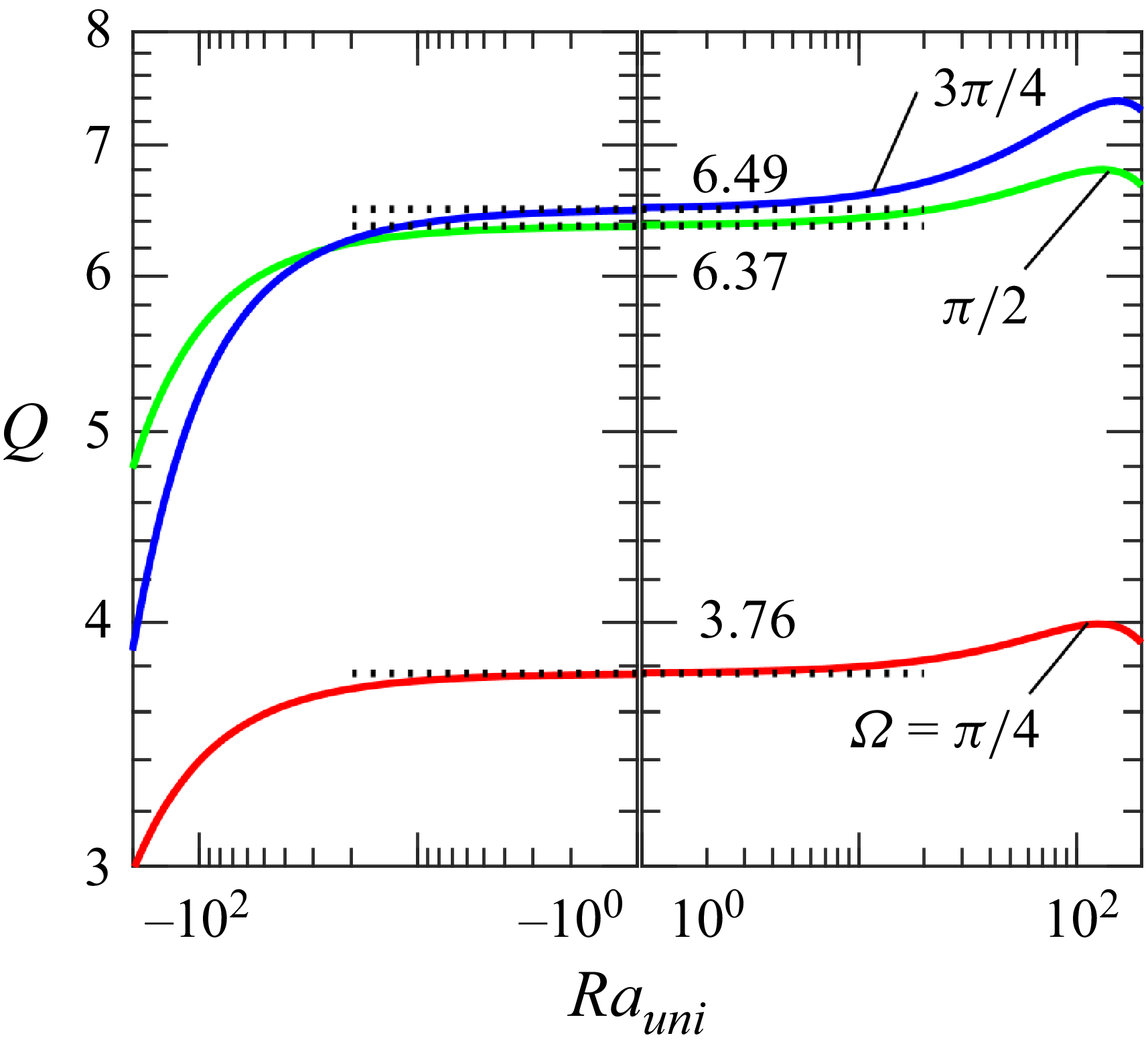
 $\textit{Ra}_{\!p}=500$
,
 $\textit{Ra}_{\textit{uni}}=0$
and
 $\alpha =1.$
The flow conditions in these figures are marked in figure 5 using magenta circles. The temperature was normalized to its maximum. An example of the magnitude of the stream function is shown in the figure corresponding to
 $A=0.5$
and
 $\varOmega =\pi /4$
.

As there is no mean horizontal pressure gradient, the net flow is driven by the pressure forces acting on the fluid at the grooved plate. The distributions and mean values of these forces change significantly with the position of the hot spot relative to the groove peak, as illustrated in figure 4. The distributions are symmetric for
 $\varOmega =0,\pi ,$
yielding zero mean and being unable to drive the net flow. For a small groove amplitude
 $(A=0.5)$
, placing a hot spot on the left-hand side of the groove peak
 $(\varOmega =\pi /4$
, figure 4
a) results in a positive pressure force at the downwelling (in the flow direction) part of the groove, which dominates the opposing force generated on the upwelling part. Increasing the phase difference to
 $\varOmega =\pi /2$
results in a positive force generated for the whole groove. Further increasing the phase difference to
 $\varOmega =3\pi /4$
results in negative forces acting on the downwelling part and positive forces acting on the upwelling part, with the latter dominating. Increasing groove amplitude to
 $A=1.5$
retains the qualitative character of distributions of these forces, with their amplitudes increasing almost by a factor of four (figure 4
b). Further increase of the groove amplitude to
 $A=2.5$
(figure 4
c) follows the same trend, with the amplitudes of pressure forces rising by another factor of almost two.
Variations of the x-component of the pressure force acting on the fluid at the lower plate (
 $\sigma _{xp,L}$
) for
 $\textit{Ra}_{\!p}=500$
,
 $\textit{Ra}_{\textit{uni}}=0$
,
 $\alpha =1$
and
 $A=0.5$
(a),
 $1.5$
(b) and
 $2.5$
(c). The dashed lines show the mean values for
 $\varOmega =\pi /4$
(green),
 $\pi /2$
(blue)
 $3\pi /4$
(cyan), and are 10.82, 17.40, 15.95 in (a), 22.00, 34.94, 32.09 in (b) and 22.15, 33.42, 27.04 in (c). The flow conditions in these figures are marked in figure 5 using magenta circles.

The variations of flow rate
 $Q$
as a function of the groove amplitude
 $A$
and the phase shift
 $\varOmega$
in (a), and as a function of the groove amplitude for selected
 $\varOmega$
’s in (b). All results are for
 $\alpha =1$
,
 $\textit{Ra}_{\!p}=500$
and
 $\textit{Ra}_{\textit{uni}}=0$
. The red solid line in (a) identifies conditions leading to the largest flow rate for a specified
 $A,$
with the blue triangle identifying the largest flow rate, i.e.
 $(\varOmega ,A)=(0.65\pi ,1.38)$
. In (a), the magenta circles mark the flow conditions used in figure 3, the horizontal green solid, dashed, and dashed–dotted lines mark the flow conditions used in figure 6(a), and the vertical blue solid, dashed and dashed–dotted lines identify the conditions used in (b).

Variations of the flow rate
 $Q$
for
 $\alpha =1$
,
 $\textit{Ra}_{\!p}=500$
and
 $\textit{Ra}_{\textit{uni}}=0$
(a) as a function of the phase shift
 $\varOmega$
and (b) as a function of the heating intensity
 $\textit{Ra}_{\!p}$
for
 $\varOmega =\pi /2$
. The flow conditions used in (a) are indicated in figures 5 and 7 using horizontal green solid, dashed and dashed–dotted lines, and those used in (b) are indicated in figure 7 using vertical blue solid, dashed and dashed–dotted lines. Panel (b) also displays variations of
 $Q$
for a special case with
 $\varOmega =0.97\pi$
and
 $A=2.5$
where the solid light-green line corresponds to the positive
 $Q$
and dashed light-green line to negative
 $Q$
. The red square in the top right-hand corner of (b) identifies the flow conditions used in figure 8.

The variations of flow rate
 $Q$
as a function of the phase shift
 $\varOmega$
and heating intensity
 $\textit{Ra}_{\!p}$
for
 $\alpha =1$
,
 $\textit{Ra}_{\textit{uni}}=0$
and
 $A=0.5$
(a),
 $1.5$
(b) and
 $2.5$
(c). The red curves identify conditions leading to the largest flow rate for a specified
 $\textit{Ra}_{\!p}$
. The solid, dashed, and dashed–dotted horizontal green lines identify the flow conditions used in figure 6(a). The solid, dashed and dashed–dotted vertical blue lines identify the flow conditions used in figure 6(b). The vertical solid light-green line in (c) identifies the flow conditions used in figure 6(b). The red square in the top right-hand corner of (c) identifies conditions used in figure 8. The magenta circles mark the flow conditions used in figure 3.

Illustration of the flow response for
 $\textit{Ra}_{\!p}=1000$
,
 $\textit{Ra}_{\textit{uni}}=0$
,
 $\alpha =1$
,
 $A=2.5$
,
 $\varOmega =0.97\pi$
. The flow and temperature fields are displayed in (a), the flow and pressure fields are displayed in (b) and the distributions of the x-component of pressure force and the x-component of shear force at the lower plate are displayed in (c). The flow conditions used in these figures are indicated in figures 6(b) and 7(c) with red squares.

The effects of the groove amplitude are explicitly illustrated in figure 5. The flow rate
 $Q$
increases proportionally to the groove amplitude
 $A$
until
 $A\approx 0.2$
(see figure 5
b), then this increase slows down with
 $Q$
reaching a maximum around
 $A=1-1.5$
, and begins to decrease with a further rise of
 $A$
. The decrease of
 $Q$
is due to a reduction in the effective slot opening as the tip of the groove approaches the opposite wall, increasing flow resistance, which we shall refer to as flow choking. The reader may note that the net flow will be eliminated for
 $A=4$
as the peak of the groove meets the upper plate. The relative position of the groove peaks and hot spots, giving the largest flow rate, changes with
 $A$
. It corresponds to
 $\varOmega =\pi /2$
at small groove amplitudes, increases up to approximately
 $\varOmega \approx 0.65\pi$
for
 $A\approx 1.38$
, which approximately corresponds to the largest flow rate, and then decreases back to
 $\varOmega =\pi /2$
with a further increase of
 $A$
(see figure 5
a).
The effects of the relative position of the hot spots and groove peaks are explicitly illustrated in figure 6. The largest flow rate is obtained for
 $\varOmega$
between
 $\pi /2$
and
 $3\pi /4$
(see figure 6
a). This flow rate increases proportionally to
 $\textit{Ra}_{\!p}$
in the heating range considered in this study (see blue curves in figure 6
b).
A more global look at variations of the flow rate as a function of various flow parameters is provided in figure 7. The most effective positioning of the hot spot changes from
 $\varOmega \approx \pi /2$
at small heating intensity, regardless of the groove amplitude
 $A$
, up to
 $\varOmega \approx 11\pi /16$
at the highest heating rate of
 $\textit{Ra}_{\!p}=1000$
considered in this study. An increase in the groove amplitude reduces the change of the most effective
 $\varOmega$
associated with a rise in
 $\textit{Ra}_{\!p}$
(see figure 7
c).
Peculiar flows occur for
 $\varOmega \approx \pi$
and high groove amplitudes as illustrated in figure 8. These flow conditions are marked using light-green squares in figures 6 and 7. The flow rate increases with
 $\textit{Ra}_{\!p}$
, as illustrated by the light-green line in figure 6(b), and then decreases and changes direction. The flow, pressure and temperature patterns corresponding to the reversed flow are illustrated in figure 8. The flow field exhibits two large vortical rolls, with a narrow stream tube meandering between them and directed towards the left-hand side. They demonstrate that the bottom of the trough, where pressure is low, plays a marginal role in the overall fluid movement. Comparisons with the patterns shown in the right column of figure 3(a iii–e iii) demonstrate a qualitative, rapid change in the flow character with increasing heating intensity. The resulting flow generates very large changes in the shear acting on the plates, as shown in figure 8(c).
The flow rate changes with the groove wavenumber as illustrated in figure 9. The most effective wavenumber is
 $\alpha \approx 0.8$
for all flow conditions considered, but the most effective relative position of heating and groove patterns changes with
 $\alpha$
, and varies between
 $\varOmega \approx \pi /2$
when
 $\alpha =0.1$
, to
 $\varOmega \approx 5\pi /8$
when
 $\alpha \approx 1$
and back to
 $\varOmega \approx 3\pi /8$
when
 $\alpha \approx 5$
(see figure 9
a). The flow rate decreases proportionally to
 $\alpha$
when
 $\alpha \rightarrow 0$
(see figure 9
b), similarly as in the case of small groove amplitudes (Abtahi & Floryan Reference Floryan, Haq and Panday2017). It decreases proportionally to
 $\alpha ^{-3}$
when
 $\alpha \rightarrow \infty$
(see figure 9
b); the character of variations in the large
 $\alpha$
limit was established through numerical experiments.
Variations of the flow rate
 $Q$
as a function of the wavenumber
 $\alpha$
and the phase shift
 $\varOmega$
in (a) and as a function of the wavenumber
 $\alpha$
for selected
 $\varOmega$
’s in (b). All results are for
 $\textit{Ra}_{\!p}=500$
,
 $\textit{Ra}_{\textit{uni}}=0$
and
 $A=1.5.$
The red solid line in (a) identifies conditions leading to the largest flow rate for a specified
 $\alpha ,$
with the blue triangle identifying the conditions for the largest flow rate, i.e.
 $(\varOmega ,\alpha )=(0.65\pi ,0.815)$
. The vertical blue solid, dashed and dashed–dotted lines in (a) identify the flow conditions used in (b). The horizontal green dashed line in (a) identifies the condition used in figure 6(a), and cyan circles identify conditions used figures 3(a ii), 3(b ii), 3(c ii), 3(d ii) and 3(e ii). The blue square identifies conditions used in figure 10.

Details of the flow for
 $\textit{Ra}_{\!p}=500$
,
 $\textit{Ra}_{\textit{uni}}=0$
,
 $\alpha =5$
,
 $A=1.5$
,
 $\varOmega =\pi /2$
. The flow and temperature fields are shown in (a). The y-distributions of the x-velocity component u (solid curves) and the temperature
 $\theta$
(dash–dot curves) are shown in (b). The flow conditions used in these figures are indicated in figure 9 with blue squares.

The typical flow and temperature fields, as well as distributions of the longitudinal velocity component for large wavenumbers, are displayed in figure 10. The flow pattern is nearly symmetric with respect to the groove trough (see figure 10
a), with the fluid jetting to the right above groove peaks, and similar jetting at
 ${x}/{\lambda }={1}/{4},{3}/{4}$
and a jetting to the right-hand side near the groove bottom and to the left-hand side near the upper plate above the groove trough (see figure 10
b). The temperature pattern is nearly antisymmetric with respect to the groove trough.
Creating purely periodic heating is very challenging, so it would be helpful to determine the effect of any mean temperature difference between the plates. This can be done by adding a uniform heating/cooling component to the lower plate. Results displayed in figure 11 demonstrate that such heating has a marginal effect on the flow rate, with cooling decreasing the flow rate and heating increasing it (see figure 11) within the heating range considered in this analysis.
Variations of the flow rate
 $Q$
as a function of the uniform heating intensity
 $\textit{Ra}_{\textit{uni}}$
for
 $\alpha =1$
,
 $A=1.5$
and
 $\textit{Ra}_{\!p}=500.$
.

4. Flow generated by heated grooves placed on both plates
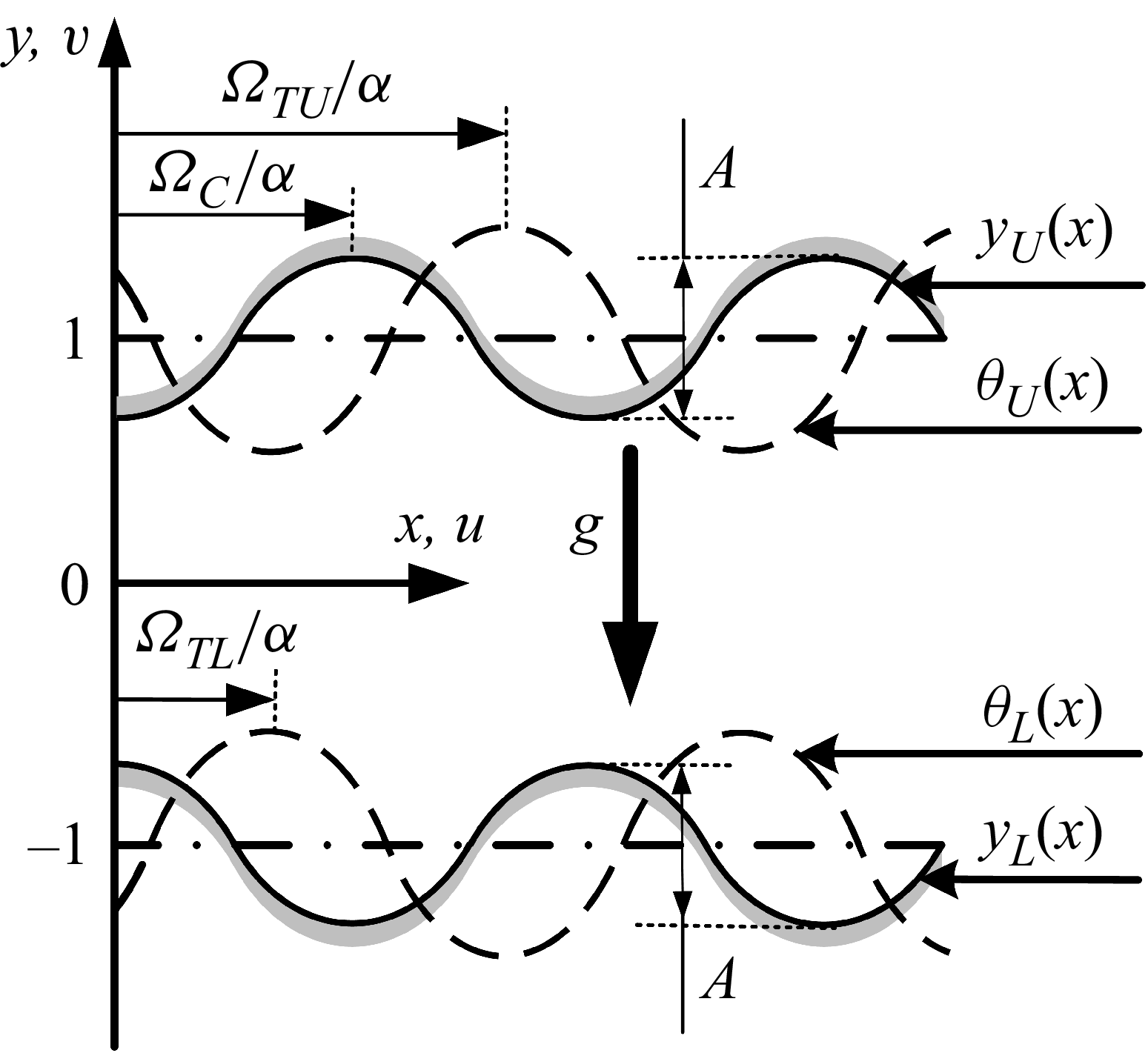
One may expect that equipping both plates with heated grooves should increase the flow rate. To quantify this effect, consider a horizontal slot formed by two corrugated plates sketched in figure 12, whose geometry is described by the following relations:
 \begin{equation}y_{L}(x)=-1+\frac{1}{2}\mathrm{A}\cos \alpha x,\quad y_{U}(x)=1+\frac{1}{2}A\cos (\alpha x+\varOmega _{C}),\end{equation}
where the upper and lower grooves were assumed to have the same amplitudes to reduce the number of parameters, and the phase shift
 $\varOmega _{C}$
describes their relative position. Variations of
 $\varOmega _{C}$
alter the geometry of the slot, with the largest and smallest possible slot openings being
 $2+A$
and
 $2-A$
, respectively.
A schematic of the flow system. The slot is located between
 $y_{L}(x)$
and
 $y_{U}(x)$
. The phases
 $\varOmega _{C}$
,
 $\varOmega _{\textit{TL}}$
and
 $\varOmega _{\textit{TU}}$
define the relative positions of the upper and lower grooves, and the grooves and the heating at the lower and upper plates, respectively.

The lower and upper plates are heated, resulting in the plates' temperature distributions being of the form
 \begin{equation}\theta _{L}(x)={\textit{Ra}_{\textit{uni}}}+\frac{1}{2}\textit{Ra}_{\!p}\cos (\alpha x+\varOmega _{\textit{TL}}),\quad \theta _{U}(x)=\frac{1}{2}\textit{Ra}_{\!p}\cos (\alpha x+\varOmega _{\textit{TU}}).\end{equation}
As a multitude of geometries can be created by varying
 $\varOmega _{\mathrm{C}}$
, the discussion is focused on two limiting cases, i.e. a wavy slot
 $(\varOmega _{\mathrm{C}}=0)$
and a converging–diverging slot
 $(\varOmega _{\mathrm{C}}=\pi )$
, and an in between case corresponding to
 $\varOmega _{\mathrm{C}}=\pi /2$
. The discussion is limited to the same heating intensity for both plates to avoid multiplying cases.
4.1. Wavy slot
The wavy slot is formed by setting the phase difference
 $\varOmega _{\mathrm{C}}$
to zero. The presentation begins with the mean plates’ temperatures being identical, i.e.
 $\textit{Ra}_{\textit{uni}}=0$
.
Variations of the flow rate
 $Q$
as a function of different positionings of the upper and lower heating patterns are illustrated in figure 13(a). The flow response is symmetric with respect to the diagonal emerging from the left-hand lower corner
 $(\varOmega _{\textit{TL}}=\varOmega _{\textit{TU}})$
and antisymmetric with respect to the diagonal emerging from the right-hand lower corner
 $(\varOmega _{\textit{TU}}=2\pi -\varOmega _{\textit{TL}})$
. As a result, it is sufficient to analyse the parameter range identified in yellow in figure 13(a), as flow properties for the remaining range can be inferred from the symmetry properties. Variations of
 $\varOmega _{\textit{TL}}$
and
 $\varOmega _{\textit{TU}}$
lead to significant changes in the flow rate, including a shift in the flow direction, with the maximum
 $Q$
of 15.30 achieved using
 $(\varOmega _{\textit{TL}},\varOmega _{\textit{TU}})\approx (3\pi /4,3\pi /4)$
. The corresponding flow and temperature fields displayed in figure 14 demonstrate that the heating is concentrated in the upwelling segment of the slot (in the flow direction), producing a positive chimney effect, and cooling in the downwelling segment, producing a negative chimney effect (Naylor et al. Reference Novak and Floryan1991; Straatman et al. Reference Straatman, Tarasuk and Floryan1993, Reference Straatman, Tarasuk and Floryan1994; Novak & Floryan Reference Novak and Floryan1995; Shahin & Floryan Reference Shahin and Floryan1999), with both effects reinforcing each other and producing a smooth flow with no separation bubbles. Multiple flow-field configurations can be generated for the same conditions over a specific range of parameters, as illustrated in figure 13(b). This issue will be discussed in detail later in this presentation.
Variations of the flow rate
 $Q$
as a function of the phase shift
 $\varOmega _{\textit{TL}}$
and
 $\varOmega _{\textit{TU}}$
in a wavy slot
 $(\varOmega _{\mathrm{C}}=0)$
for
 $\alpha =1$
,
 $A=1.5$
,
 $\textit{Ra}_{\!p}=500$
and
 $\textit{Ra}_{\textit{uni}}=0$
. In (a), the red circle identifies the best positioning of the heating patterns leading to the largest flow rate, i.e.
 $(\varOmega _{\textit{TL}},\varOmega _{\textit{TU}})\approx (3\pi /4,3\pi /4)$
. The black circles and triangles identify the flow conditions used in figures 15 and 16, respectively, and the horizontal red, green and blue dotted lines identify the flow conditions used in figure 17. The beige strip identifies conditions where multiple solutions exist (see text for details). Variations of
 $Q$
as a function of
 $\varOmega _{\textit{TL}}=2\pi -\varOmega _{\textit{TU}}$
, i.e. along the diagonal from the bottom right-hand corner to the centre in (a), are illustrated in (b). A black filled-in circle identifies the bifurcation point. The blue square and triangle identify the flow condition used in figures 18(c) and 18(d).

The flow and temperature field corresponding to the highest flow rate in a wavy slot
 $(\varOmega _{\mathrm{C}}=0)$
for
 $\alpha =1$
,
 $A=1.5$
,
 $\textit{Ra}_{\!p}=500$
,
 $\textit{Ra}_{\textit{uni}}=0, \varOmega _{\textit{TL}}=3\pi /4$
,
 $\varOmega _{\textit{TU}}=3\pi /4$
. These flow conditions are identified with a red circle in figure 13(a).

Detailed discussion of the flow and temperature field topologies begins with conditions corresponding to the bottom of figure 13(a), i.e.
 $\varOmega _{\textit{TU}}=0$
(position of the upper heating pattern is fixed with a hot spot located at
 $x=0$
while the lower pattern changes its location). The flow field is symmetric with respect to
 ${x}/{\lambda }=0.5$
when
 $\varOmega _{\textit{TL}}=0$
(the
 $x$
-positions of the upper and lower hot spots are the same, figure 15
a) and consists of two large rolls with the fluid drawn away from the lower trough along the lower plate. The flow field is also symmetric when
 $\varOmega _{\textit{TL}}=\pi$
(lower hot spot is at
 $x/\lambda =0.5$
; figure 15
c) and involves four rolls. Positioning of the lower hot spot between these two locations results in a net flow to the right-hand side when
 $\varOmega _{\textit{TL}}=\pi /2$
(figure 15
b) and to the left-hand side when
 $\varOmega _{\textit{TL}}=3\pi /2$
(figure 15
d).
The flow and temperature fields in a wavy slot
 $(\varOmega _{\mathrm{C}}=0)$
for
 $\textit{Ra}_{\!p}=500$
,
 $\textit{Ra}_{\textit{uni}}=0$
,
 $\alpha =1$
,
 $A=1.5$
and
 $\varOmega _{\textit{TU}}=0$
for
 $\varOmega _{\textit{TL}}=0,\pi /2,\pi ,3\pi /2$
in (a), (b), (c), (d), respectively. The flow conditions in these figures are identified in figure 13(a) using black circles. The temperature was normalized to its maximum.

The flow and temperature fields in a wavy slot
 $(\varOmega _{\mathrm{C}}=0)$
for
 $\textit{Ra}_{\!p}=500$
,
 $\textit{Ra}_{\textit{uni}}=0$
,
 $\alpha =1$
,
 $A=1.5$
, for
 $(\varOmega _{\textit{TL}},\varOmega _{\textit{TU}})=(\pi /2,\pi /2),(\pi ,\pi /2),(3\pi /2,\pi /2),(\pi ,\pi )$
in (a–d). The flow conditions in these figures are identified in figure 13(a) using black triangles. The temperature was normalized to its maximum.

Variations of the flow rate
 $Q$
as a function of the phase shift
 $\varOmega _{\textit{TL}}$
for selected values of
 $\varOmega _{\textit{TU}}$
for
 $\alpha =1$
,
 $A=1.5$
,
 $\textit{Ra}_{\!p}=500$
and
 $\textit{Ra}_{\textit{uni}}=0$
for a wavy slot
 $(\varOmega _{C}=0)$
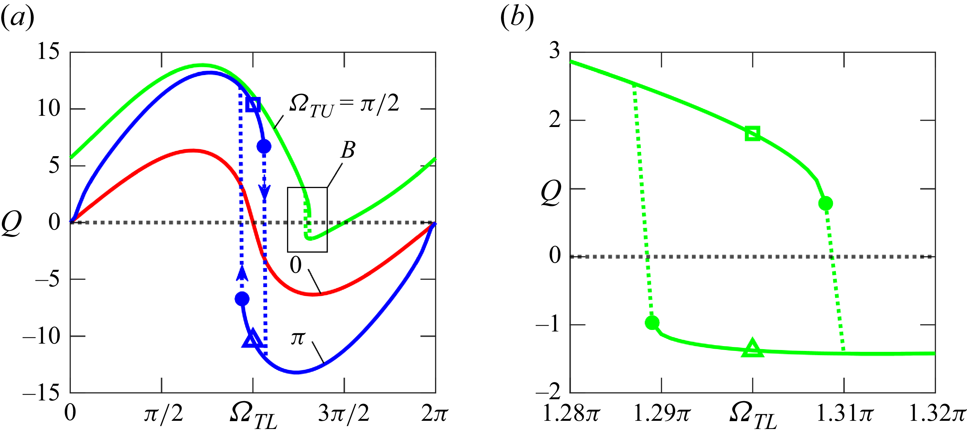
. Panel (b) displays the enlargement of the box marked in (a). Squares and triangles identify the flow conditions used in figure 18. Filled-in circles identify limit points. The flow and temperature fields corresponding to blue symbols in (a) are displayed in figures 18(c) and 18(d), and corresponding to green symbols in (b) are displayed in figures 18(a) and 18(b).

The flow and temperature fields for
 $\varOmega _{C}=0$
,
 $\alpha =1$
,
 $A=1.5$
,
 $\textit{Ra}_{\!p}=500$
,
 $\textit{Ra}_{\textit{uni}}=0$
. Two possible flow patterns for
 $\varOmega _{\textit{TU}}=\pi /2$
and
 $\varOmega _{\textit{TL}}=1.3\pi$
are displayed in (a) and (b), while two possible patterns for
 $\varOmega _{\textit{TU}}=\varOmega _{\textit{TL}}=\pi$
are displayed in (c) and (d). The flow conditions used in these figures are identified in figure 17, denoted by squares and triangles.

Examples of flow patterns corresponding to conditions in the interior of the yellow triangle in figure 13(a) are displayed in figure 16. The patterns are simple in figures 16(a) and 16(b), but become complex in figures 16(c) and 16(d), especially for figure 16(c). In figure 16(c), flow streams form along the top and bottom plates with a central recirculating zone in between. The upper stream carries more fluid to the right-hand side than the lower stream carries to the left-hand side, producing a net rightward flow (see figure 13
a). A similar flow pattern is also observed in figures 18(a) and 18(b). The conditions used in the last two figures correspond to the left-hand diagonal in figure 13(a), which serves as the antisymmetry axis. The solution is non-unique for conditions near this axis (the beige diagonal strip in figure 13
a), as illustrated in figure 17. Consider
 $\varOmega _{\textit{TU}}=\pi$
(blue line in figure 17
a), as
 $\varOmega _{\textit{TL}}$
increases from zero, the flow rate increases and reaches a maximum near
 $\varOmega _{\textit{TL}}\approx 3\pi /4$
and then starts to decrease, reaching a limit point at
 $\varOmega _{\textit{TL}}=1.06\pi$
. Further increase of
 $\varOmega _{\textit{TL}}$
causes an abrupt change in the flow pattern, including a reversal in the flow direction, then the flow rate reaches a negative maximum, and eventually decreases to zero when
 $\varOmega _{\textit{TL}}=2\pi$
. Reversing the direction of changes of
 $\varOmega _{\textit{TL}}$
, i.e. reducing
 $\varOmega _{\textit{TL}}$
from
 $2\pi$
down to zero, demonstrates the formation of another limit point at
 $\varOmega _{\textit{TL}}=0.94\pi$
creating a hysteresis loop where two different flow patterns may exist for the same flow conditions (see figures 17
a, 18
c and 18
d). A qualitatively similar character of the flow response is observed for
 $\varOmega _{\textit{TU}}=\pi /2$
(green line in figure 17) with the dual solutions occurring near
 $\varOmega _{\textit{TL}}=1.3\pi$
(see figures 17
b, 18
a and 18
b).
Effects of variations of the groove amplitude are illustrated in detail in figure 19(a). The system produces a larger driving force due to an increase of
 $A$
. At the same time, an increase of
 $A$
changes the channel geometry by bringing both plates together in a nearly parallel manner, forming a wavy channel whose effective length (compared with the length of a straight channel with the same x-extent) is larger, thereby increasing flow resistance. For small enough amplitudes, the first effect dominates, and
 $Q$
increases proportionally to
 $A$
(see figure 19
b). This growth slows down with further increases in
 $A$
, as the second effect begins to dominate, reducing the flow rate. The magnitude of slowing down changes significantly with the position of the hot spots. The most effective position of hot spots is identified with a cyan line in figure 19(a), and it is
 $\varOmega _{\textit{TL}}=\varOmega _{\textit{TU}}\approx \pi /2$
for small amplitudes and increases to
 $\varOmega _{\textit{TL}}=\varOmega _{\textit{TU}}\approx 3\pi /4$
for the largest amplitude considered. The case of
 $\varOmega _{\textit{TL}}=\varOmega _{\textit{TU}}=\pi$
is special as there is no net horizontal flow until the amplitude reaches a certain critical magnitude (see figures 19
a and 19
c). Then, the symmetric flow becomes unstable and bifurcates, creating two flows with opposite horizontal flow rates, as depicted in figures 18(c) and 18(d).
Variations of the flow rate
 $Q$
as a function of the groove amplitude
 $A$
and the phase shifts
 $\varOmega _{\textit{TL}}=\varOmega _{\textit{TU}}$
for a wavy slot (
 $\varOmega _{C}=0$
) and
 $\alpha =1$
,
 $\textit{Ra}_{\!p}=500$
,
 $\textit{Ra}_{\textit{uni}}=0.$
The beige strip in (a) identifies conditions where multiple solutions exist (see text for details). The solid cyan lines identify the phase shift
 $\varOmega _{\textit{TL}}=\varOmega _{\textit{TU}}$
producing the largest flow rate for a specified
 $A$
. The red, green, blue and magenta dotted lines identify flow conditions used in (b). Panel (c) displays variations of
 $Q$
as a function of
 $A$
for
 $\varOmega _{\textit{TL}}=\varOmega _{\textit{TU}}=\pi$
. The magenta triangle and square in (c) identify conditions used in figures 18(c), 18(d) and 17(a).

Effects of variations of the heating intensity are illustrated in detail in figure 20(a). The flow rate
 $Q$
initially increases proportionally to
 $\textit{Ra}_{\!p}$
(see figure 20
b) and then its growth slows, and its value approaches a constant with a further increase of
 $\textit{Ra}_{\!p}$
. Variations of
 $Q$
are similar for all positions of hot spots except when they are placed at a location corresponding to the trough of the lower groove
 $(\varOmega _{\textit{TL}}=\varOmega _{\textit{TU}}=\pi )$
. In this case, the flow is symmetric for sufficiently weak heating, producing no net horizontal flow. Increase of heating intensity results in system bifurcation, as illustrated in figure 20(c), producing either negative or positive net flows for the otherwise identical conditions, with the resulting flow fields depicted in figures 18(c) and 18(d). The most effective position of hot spots is identified with a cyan line in figure 20(a), and it is
 $\varOmega _{\textit{TL}}=\varOmega _{\textit{TU}}\approx \pi /2$
for small amplitudes and increases to
 $\varOmega _{\textit{TL}}=\varOmega _{\textit{TU}}\approx 3\pi /4$
for the largest amplitude considered.
Variations of the flow rate
 $Q$
as a function of the heating intensity
 $\textit{Ra}_{\!p}$
and the phase shifts
 $\varOmega _{\textit{TL}}=\varOmega _{\textit{TU}}$
for a wavy slot
 $(\varOmega _{C}=0)$
and
 $\alpha =1$
,
 $A=1.5$
,
 $\textit{Ra}_{\textit{uni}}=0$
. The beige strip in (a) identifies conditions where multiple solutions exist (see text for details). The cyan line identifies conditions leading to the largest flow rate for a specified
 $\textit{Ra}_{\!p}$
. The red, green, blue and magenta dotted lines identify the flow conditions used in (b). Panel (c) displays variations of
 $Q$
as a function of
 $\textit{Ra}_{\!p}$
for
 $\varOmega _{\textit{TL}}=\varOmega _{\textit{TU}}=\pi$
. The magenta triangle and square in (c) identify conditions used in figures 18(c), 18(d) and 17(a).

Effects of variations of the system wavenumber are illustrated in figure 21(a). There is an optimal wavenumber that produces the largest flow rate. The optimal wavenumber is
 $\alpha \approx (0.5-0.7)$
, as illustrated in figures 21(a) and 21(b), and it changes marginally with the location of the hot spots. A reduction of
 $\alpha$
(long wavelength systems) decreases
 $Q$
proportionally to
 $\alpha ,$
while an increase of
 $\alpha$
(short wavelength systems) reduces
 $Q$
proportionally to
 $\alpha ^{-3}$
, as illustrated in figure 21(b). The system response is peculiar for
 $\varOmega _{\textit{TL}}=\varOmega _{\textit{TU}}=\pi$
. There is no net flow if the system wavenumber is either too small or too large; two flows, giving opposite flow rates, occur between these limits, as illustrated in figure 21(c), with the possible flow fields shown in figures 18(c) and 18(d).
Variations of the flow rate
 $Q$
as a function of the wavenumber
 $\alpha$
and the phase shifts
 $\varOmega _{\textit{TL}}=\varOmega _{\textit{TU}}$
for a wavy slot
 $(\varOmega _{C}=0)$
and
 $\alpha =1$
,
 $A=1.5$
,
 $\textit{Ra}_{\!p}=500$
,
 $\textit{Ra}_{\textit{uni}}=0$
. The beige strip in (a) identifies conditions where multiple solutions exist (see text for details). The cyan curves identify conditions leading to the largest flow rate for a specified
 $\alpha$
, and the red, green, blue and magenta dotted lines identify the flow conditions used in (b). The data in (c) are for
 $\varOmega _{\textit{TL}}=\varOmega _{\textit{TU}}=\pi$
. Filled-in circles identify bifurcation points. Flow and temperature fields corresponding to conditions identified with a magenta triangle and square are displayed in figures 18(c) and 18(d).

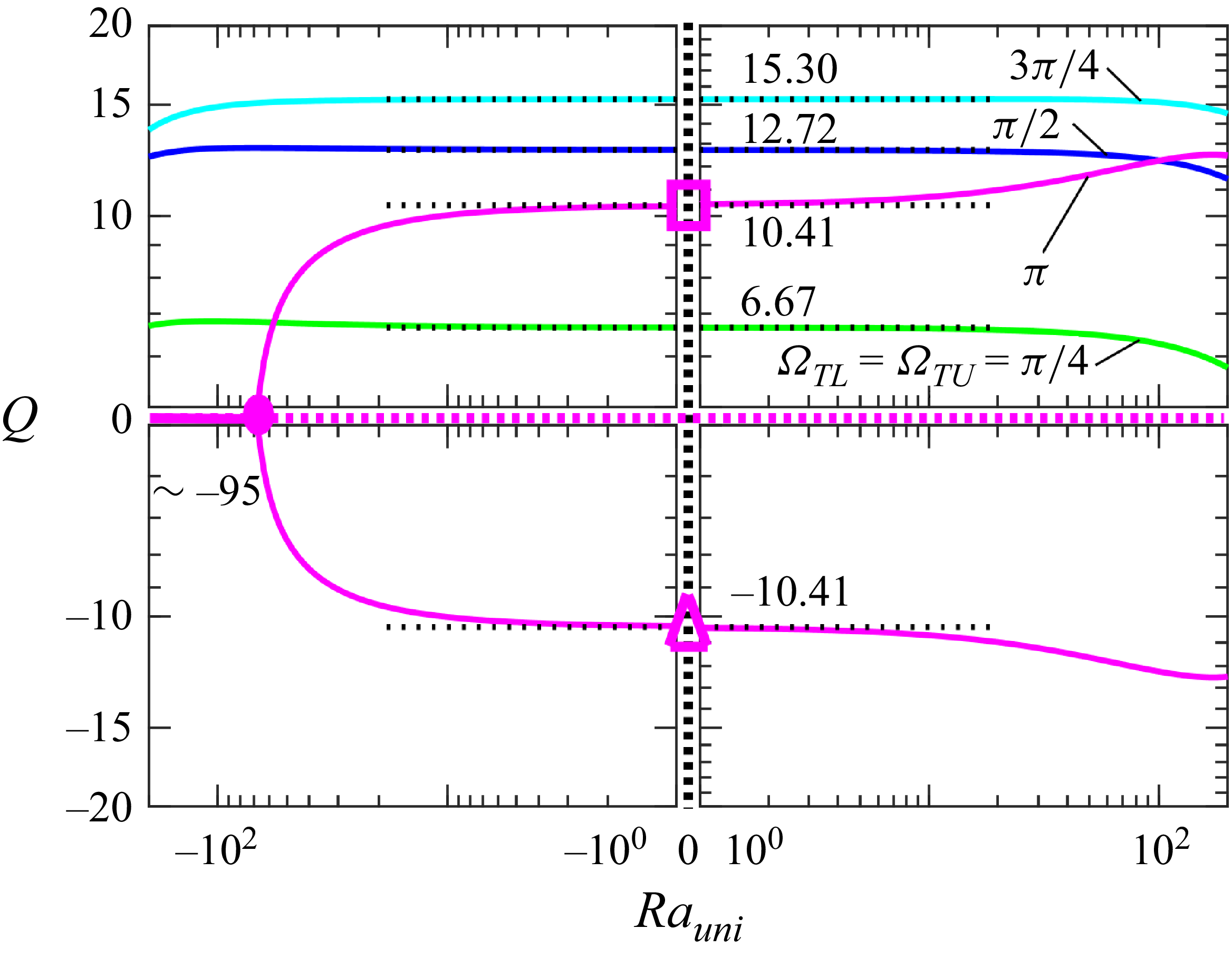
This discussion is completed by assessing the effect of a uniform heating component. Here
 $Q$
changes marginally in the range of variations of
 $\textit{Ra}_{\textit{uni}}$
that are of interest in this analysis, except for
 $\varOmega _{\textit{TL}}=\varOmega _{\textit{TU}}\approx \pi$
as illustrated in figure 22. In this case, cooling of the lower plate results in a complete elimination of the net flow for
 $\textit{Ra}_{\textit{uni}}\lt \sim -95$
. As
 $\textit{Ra}_{\textit{uni}}$
increases from −95, the system goes through a bifurcation that can produce a positive or negative
 $Q$
for otherwise identical conditions.
Variations of the flow rate
 $Q$
as a function of the uniform heating intensity
 $\textit{Ra}_{\textit{uni}}$
for a wavy slot
 $(\varOmega _{C}=0)$
and
 $\alpha =1$
,
 $A=1.5$
,
 $\textit{Ra}_{\!p}=500$
. The filled-in circle marks the bifurcation point. Flow and temperature fields corresponding to conditions identified with a magenta triangle and square are displayed in figures 18(c) and 18(d).

Variations of the flow rate
 $Q$
as a function of the phase shifts
 $\varOmega _{\textit{TL}}$
and
 $\varOmega _{\textit{TU}}$
for a converging–diverging slot
 $(\varOmega _{\mathrm{C}}=\pi )$
for
 $\alpha =1$
,
 $\textit{Ra}_{\!p}=500$
,
 $\textit{Ra}_{\textit{uni}}=0$
,
 $A=1.5$
. The red circle identifies the overall best conditions leading to the largest flow rate, which is
 $ (\varOmega _{\textit{TL}},\varOmega _{\textit{TU}} )\approx ({3\pi }/{2},{\pi }/{2} )$
. The black circles in figure identify the flow conditions used in figure 25.

4.2. Converging–diverging slot
The converging–diverging slot corresponds to
 $\varOmega _{\mathrm{C}}=\pi$
. The discussion begins with the slot formed by plates with the same mean temperatures, i.e.
 $\textit{Ra}_{\textit{uni}}=0$
. The reader may note that the slot evolves towards a rectangular cavity with lateral walls kept at different temperatures as
 $A\rightarrow 4$
. Such cavities have been frequently studied in the past (Paolucci Reference Paolucci1994; Hussein et al. Reference Novak and Floryan2014; Liu & Zhang Reference Novak and Floryan2022).
Variations of the flow rate
 $Q$
as a function of different positionings of the upper and lower heating patterns are illustrated in figure 23 for
 $A=1.5$
. The flow response has symmetries in the sense that the transformations
 $\varOmega _{\textit{TU}}\rightarrow 2\pi -\varOmega _{\textit{TU}}$
and
 $\varOmega _{\textit{TL}}\rightarrow 2\pi -\varOmega _{\textit{TL}}$
result in
 $Q\rightarrow -Q$
. All information about flow responses can be deduced by considering the range of parameters identified in yellow in figure 23. In general, the magnitude of the flow rate achieved in this geometry is by an order of magnitude smaller than that achieved with a wavy slot. Conditions leading to the largest
 $Q$
are
 $ (\varOmega _{\textit{TL}},\varOmega _{\textit{TU}} )= ({3\pi }/{2},{\pi }/{2} )$
(see red circle in figure 23) and produce
 $Q=-1.2$
.
The flow and temperature fields for a converging–diverging slot
 $(\varOmega _{\mathrm{C}}=\pi )$
for
 $\textit{Ra}_{\!p}=500$
,
 $\textit{Ra}_{\textit{uni}}=0$
,
 $\alpha =1$
,
 $A=1.5$
and
 $\varOmega _{\textit{TU}}=\varOmega _{\textit{TL}}=0$
in (a) and
 $\varOmega _{\textit{TU}}=\varOmega _{\textit{TL}}=\pi$
in (b). The temperature was normalized to its maximum.

The flow and temperature fields for a converging–diverging slot
 $(\varOmega _{\mathrm{C}}=\pi )$
for
 $\textit{Ra}_{\!p}=500$
,
 $\textit{Ra}_{\textit{uni}}=0$
,
 $\alpha =1$
,
 $A=1.5$
and
 $(\varOmega _{\textit{TL}},\varOmega _{\textit{TU}})=(0,{\pi }/{2}),({\pi }/{2},{\pi }/{2}),(\pi ,{\pi }/{2}),({3\pi }/{2},{\pi }/{2})$
in (a), (b), (c), (d), respectively. The temperature was normalized to its maximum. The flow conditions used in these figures are marked with black circles in figure 23.

There is no net horizontal flow when hot spots overlap with the largest and smallest slot openings, as illustrated in figure 24. Examples of flow and temperature fields for other positions of hot spots displayed in figure 25 demonstrate that fluid movement is mainly confined to the largest slot opening, producing a marginal net horizontal flow rate and resemble flow in rectangular cavities whose lateral sides are kept at different temperatures (Paolucci Reference Paolucci1994; Hussein et al. Reference Novak and Floryan2014; Liu & Zhang Reference Novak and Floryan2022).
The variations of
 $Q$
as a function of
 $\alpha$
,
 $\textit{Ra}_{\!p}$
and
 $A$
are qualitatively similar to the case of a wavy slot. Here
 $Q$
initially increases proportionally to
 $\textit{Ra}_{\!p}$
until flow saturation slows it down. It initially increases proportionally to
 $A$
, reaches a maximum and starts to decrease as the reduction of the minimum distance between the plates chokes the flow. It decreases proportionally to
 $\alpha$
when
 $\alpha \rightarrow 0$
and proportionally to
 $\alpha ^{-3}$
when
 $\alpha \rightarrow \infty ,$
with the largest flow rate generated for
 $\alpha \approx 1-2$
. Details of the analysis are not provided. Multiple solutions are possible for the same conditions. Still, they require a significantly higher heating intensity than wavy slots do.
Analysis of the effects of uniform heating shows marginal changes in
 $Q$
with
 $\textit{Ra}_{\textit{uni}}$
, as in the case of wavy slots, in the range of parameters considered in this study. Details are not given.
4.3. Slot with a geometry in between the wavy and converging–diverging slots
 $({\varOmega }_{{C}}= {\pi }/ {2})$

It is of interest to inquire about the system response if an ‘irregular’ slot geometry is used. The term ‘irregular’ is used here in the sense that geometry does not have any symmetries. Figure 26 illustrates the flow and temperature fields for a slot with
 $\varOmega _{C}=\pi /2$
. This series of plots corresponds to a fixed position for the upper heating pattern and varying positions for the lower pattern. It is clear that this geometry lacks symmetries, so one must investigate the full range of relevant parameters. Figure 27 illustrates variations of the flow rate
 $Q$
for the full range of possible positioning of the upper and lower heating patterns for
 $A=1.5$
. The magnitude of
 $Q$
is similar to that in a converging–diverging slot and much smaller than that achievable in the wavy slot, making this configuration of marginal interest from an application point of view. Interestingly, the variations of
 $Q$
display antisymmetry with respect to the line giving
 $Q=0$
going approximately from the right-hand lower corner to the left-hand upper corner, as marked in figure 27. The yellow colour identifies the relevant range of
 $\varOmega _{\textit{TL}}$
and
 $\varOmega _{\textit{TU}}$
, as the
 $Q$
for the remaining range can be deduced from the antisymmetric properties.
The flow and temperature fields for a slot
 $(\varOmega _{\mathrm{C}}=\pi /2)$
for
 $\textit{Ra}_{\!p}=500$
,
 $\textit{Ra}_{\textit{uni}}=0$
,
 $\alpha =1$
,
 $A=1.5$
and
 $(\varOmega _{\textit{TL}},\varOmega _{\textit{TU}})=(0,0.2975\pi ), ({\pi }/{2},0.2975\pi ), (\pi ,0.2975\pi), ({3\pi }/{2},0.2975\pi)$
in (a), (b), (c), (d), respectively. The temperature was normalized to its maximum. The flow conditions used in these figures are marked with black circles in figure 27.

Variations of the flow rate
 $Q$
as a function of the phase shifts
 $\varOmega _{\textit{TL}}$
and
 $\varOmega _{\textit{TU}}$
for a slot with
 $\varOmega _{\mathrm{C}}=\pi /2$
for
 $\alpha =1$
,
 $\textit{Ra}_{\!p}=500$
,
 $\textit{Ra}_{\textit{uni}}=0$
,
 $A=1.5$
. The red circle identifies the overall best conditions leading to the largest flow rate, which are
 $(\varOmega _{\textit{TL}},\varOmega _{\textit{TU}})\approx (0.5425\pi ,0.2975\pi )$
and
 $(1.2025\pi ,0.9575\pi )$
. The black circles identify the flow conditions used in figure 26. The blue circles identify the flow conditions used in figure 28. The cyan squares in figure identify the flow conditions used in figure 29.

The flow and temperature fields for a slot
 $(\varOmega _{\mathrm{C}}=\pi /2)$
for
 $\textit{Ra}_{\!p}=500$
,
 $\textit{Ra}_{\textit{uni}}=0$
,
 $\alpha =1$
,
 $A=1.5$
and
 $(\varOmega _{\textit{TL}},\varOmega _{\textit{TU}})=(\pi /2,\pi ),(3\pi /4,3\pi /4),(\pi ,\pi /2)$
in (a), (b) and (c), respectively. The temperature was normalized to its maximum. The flow conditions used in these figures are marked with blue circles in figure 27.

The flow and temperature fields for a slot with
 $\varOmega _{\mathrm{C}}=\pi /2$
for
 $\textit{Ra}_{\!p}=500$
,
 $\textit{Ra}_{\textit{uni}}=0$
,
 $\alpha =1$
,
 $A=1.5$
. Results for
 $(\varOmega _{\textit{TL}},\varOmega _{\textit{TU}})=(\pi /2,\pi /2),(\pi ,\pi )$
are presented in (a) and (b), respectively. The temperature was normalized to its maximum. The flow conditions used in these figures are marked with cyan squares in figure 27.

The character of the flow and temperature fields resulting in
 $Q=0$
at a few points along the lower boundary of the yellow zone in figure 27 are illustrated in figure 28. It is rather difficult to predict the forms of such fields without a detailed analysis, as the positions of the heating patterns must be coordinated to produce no net flow. Figure 29 displays the form of these fields for the conditions selected to illustrate antisymmetry of
 $Q$
. Their forms are difficult to predict, even qualitatively, without detailed analysis.
The variations of
 $Q$
as a function of
 $\alpha$
,
 $\textit{Ra}_{\!p}$
and
 $A$
are qualitatively similar to the case of a wavy and converging–diverging slots. Details of the analysis are not provided. Multiple solutions are possible for the same conditions, but require a significantly higher heating intensity. Adding a uniform heating component produces minor changes, as in the previous two cases, so no details are provided.
5. Closing remarks
Fluid pumping in a horizontal slot using the pattern interaction effect has been analysed. The field equations were solved using spectrally accurate IBC and a second-order finite-volume method. Both methods produced the same results in the parameter range where the IBC method was applicable.
The pumping method that utilizes the pattern interaction effect is a passive approach, requiring no moving parts and no external energy input beyond the use of appropriate heating patterns. The essence of the method is the use of grooves heated to achieve a proper plate-temperature pattern. Its mechanics have been described in the context of a one-grooved plate. The heating can be generated from waste heat, reducing the energy cost of pumping. The direction and intensity of the horizontal flow can be controlled by adjusting the relative positions of the heating and groove patterns. While groove positions are fixed in practical applications, the heating pattern can be easily adjusted by turning heat sources on or off or by moving heat shields. The method's effectiveness increases linearly with groove amplitude until the distance between the groove peak and the opposing plate becomes so small that the flow chokes. The best performance is achieved using groove and heating patterns with a wavenumber
 $\alpha$
of approximately 0.8. The flow rate drops off proportionally to
 $\alpha$
when
 $\alpha \rightarrow 0$
and proportionally to
 $\alpha ^{-3}$
when
 $\alpha \rightarrow \infty$
.
The use of heated grooves on both plates yields a multitude of geometries, resulting in flow rates that vary by an order of magnitude. The analysis considered three cases, i.e. the groove positions resulting in (i) the formation of wavy slots, (ii) the formation of converging–diverging slots and (iii) an in between case with an irregular geometry, that is, a geometry that does not have any symmetry properties. It was shown that wavy slots produce flow rates an order of magnitude higher than those of the other geometries, making the wavy slot the configuration of primary interest for applications. A detailed analysis of wavy slots is presented, focusing on the proper placement of heat sources on the walls. It was shown that the best performance was achieved by placing these sources halfway between the groove's extremities and using a groove wavenumber in the range of 0.5–0.7. It was found that multiple flow responses were possible for certain positions of heat sources.
The future analysis should focus on developing methods to create the required temperature patterns in an energy-efficient manner, as well as on utilizing grooves with simple shapes, such as triangular or trapezoidal, which are easy to manufacture. The theoretical questions that remain to be addressed are the system response when groove and heating patterns are characterized by different wavenumbers, which may lead to the formation of commensurate systems with very long wavelengths, as well as incommensurate systems, and the determination of the optimal groove shapes and optimal temperature distributions producing the highest flow rate.
Acknowledgements
This work was carried out with the support of the NSERC of Canada.
Declaration of interests
The authors report no conflict of interest.










 Open access

