1 Introduction
Large-eddy simulation (LES) has become a widely used numerical technique for studying turbulent flows. Turbulence often consists of a wide range of scales, which increases with the Reynolds number (Tennekes & Lumley Reference Tennekes and Lumley1972). For example, the largest scale in the atmospheric boundary layer is of the order of 1 km, while the smallest scale is of the order of 1 mm (Stull Reference Stull1988). The essence of LES is to resolve the large scales but parameterize the effects of small scales using so-called subgrid-scale (SGS) models (Pope Reference Pope2000). This is motivated by the turbulent energy cascade in which the large scales extract energy from the mean flow and transfer it to the small scales. As a result, the small scales are less affected by the boundary conditions and should thus be easier to model.
In particular, the pioneering work of Kolmogorov (Reference Kolmogorov1941) hypothesized that, if a sufficiently large scale separation exists between the largest scale and the smallest scale (i.e. the turbulent flow has a sufficiently large Reynolds number like the flow in the atmospheric boundary layer), then an inertial subrange exists in which turbulence is homogeneous and isotropic. His work further demonstrated that the turbulent kinetic energy (TKE) spectra in the inertial subrange follow the nowadays well-known ‘
 $-5/3$
’ scaling. The temperature spectra in the inertial subrange were later found to also follow such scaling by Obukhov (Reference Obukhov1949) and Corrsin (Reference Corrsin1951). The Kolmogorov–Obukhov–Corrsin theory provides the basis for developing SGS models.
The most widely used SGS model is arguably the Smagorinsky model (Smagorinsky Reference Smagorinsky1963), which is analogous to the mixing-length model proposed by Prandtl for Reynolds-averaged Naiver–Stokes (RANS) simulations. In this model, the SGS momentum (heat) flux is assumed to be proportional to the resolved velocity (temperature) gradient and the proportionality is termed SGS eddy viscosity (eddy diffusivity). The ratio of SGS eddy viscosity and eddy diffusivity is called the SGS Prandtl number, which is the focus of this study. Lilly was the first to estimate the SGS eddy viscosity based on the Kolmogorov theory (Lilly Reference Lilly1967), and others extended the analysis to the SGS eddy diffusivity (Schumann, Grötzbach & Kleiser Reference Schumann, Grötzbach, Kleiser and Kollmann1980; Moeng & Wyngaard Reference Moeng and Wyngaard1988; Mason Reference Mason1989). However, such analysis yielded an SGS Prandtl number that is both stability- (or buoyancy-) independent and scale-invariant, which is inconsistent with recent field experiments (Porté-Agel et al. Reference Porté-Agel, Parlange, Meneveau and Eichinger2001; Bou-Zeid et al. Reference Bou-Zeid, Vercauteren, Parlange and Meneveau2008; Vercauteren et al. Reference Vercauteren, Bou-Zeid, Parlange, Lemmin, Huwald, Selker and Meneveau2008; Bou-Zeid et al. Reference Bou-Zeid, Higgins, Huwald, Parlange and Meneveau2010) and new computational developments (Porté-Agel Reference Porté-Agel2004; Basu & Porté-Agel Reference Basu and Porté-Agel2006; Stoll & Porté-Agel Reference Stoll and Porté-Agel2006, Reference Stoll and Porté-Agel2008; Calaf, Parlange & Meneveau Reference Calaf, Parlange and Meneveau2011) showing that the SGS Prandtl number is stability-dependent and varies with scales.
In this study, the SGS Prandtl number is revisited by solving the SGS co-spectral budgets of momentum and heat fluxes. It is shown that even under stationary and horizontally homogeneous conditions that are often assumed to be associated with high-Reynolds-number flows in the atmospheric surface layer (ASL, which is the lowest 10 %–20 % of the atmospheric boundary layer and corresponds to the logarithmic region in wall-bounded turbulence), the SGS Prandtl number is strongly impacted by thermal stratification and the filter scale. This co-spectral budget model is in good agreement with recent field experimental data collected in the ASL and can be readily implemented in LES.
2 Theory
The SGS turbulent momentum (
 $\unicode[STIX]{x1D70F}$
) and heat (
 $h$
) fluxes are modelled as
 $$\begin{eqnarray}\displaystyle & \displaystyle \unicode[STIX]{x1D70F}_{ij}=-2c_{s}^{2}\unicode[STIX]{x1D6E5}^{2}|\widetilde{S}|\widetilde{S}_{ij}, & \displaystyle\end{eqnarray}$$
 $$\begin{eqnarray}\displaystyle & \displaystyle h_{i}=-Pr^{-1}c_{s}^{2}\unicode[STIX]{x1D6E5}^{2}|\widetilde{S}|\widetilde{D}_{i}, & \displaystyle\end{eqnarray}$$
respectively, where
 $|\widetilde{S}|=(2\widetilde{S}_{ij}\widetilde{S}_{ij})^{1/2}$
,
 $\widetilde{S}_{ij}=0.5(\unicode[STIX]{x2202}\widetilde{u_{i}}/\unicode[STIX]{x2202}x_{j}+\unicode[STIX]{x2202}\widetilde{u_{j}}/\unicode[STIX]{x2202}x_{i})$
,
 $\widetilde{D}_{i}=\unicode[STIX]{x2202}\widetilde{\unicode[STIX]{x1D703}}/\unicode[STIX]{x2202}x_{i}$
,
 $u_{i}$
is the velocity,
 $\unicode[STIX]{x1D703}$
is the potential temperature,
 $c_{s}$
is the Smagorinsky coefficient,
 $\unicode[STIX]{x1D6E5}$
is the filter scale and
 $Pr$
is the SGS Prandtl number. The tilde (
 ${\sim}$
) denotes the filtering operation.
2.1 Prior model
Theoretical derivations of the SGS Prandtl number can be found in previous studies (Schumann et al.
Reference Schumann, Grötzbach, Kleiser and Kollmann1980; Moeng & Wyngaard Reference Moeng and Wyngaard1988; Mason Reference Mason1989), all of which were built on Lilly’s thinking (Lilly Reference Lilly1967). By assuming that the inertial subrange spectra of TKE (
 $E_{TKE}=C_{TKE}\unicode[STIX]{x1D716}^{2/3}k^{-5/3}$
) and temperature (
 $E_{TT}=C_{T}\unicode[STIX]{x1D716}^{-1/3}\unicode[STIX]{x1D716}_{T}k^{-5/3}$
) apply to the wavenumber range from 0 to
 $k_{\unicode[STIX]{x1D6E5}}$
(
 $=\unicode[STIX]{x1D70B}/\unicode[STIX]{x1D6E5}$
), one arrives at
 $$\begin{eqnarray}\displaystyle & \displaystyle \tilde{S}^{2}=2\int _{0}^{k_{\unicode[STIX]{x1D6E5}}}k^{2}E_{TKE}(k)\,\text{d}k=\frac{3}{2}C_{TKE}\unicode[STIX]{x1D716}^{2/3}k_{\unicode[STIX]{x1D6E5}}^{4/3}, & \displaystyle\end{eqnarray}$$
 $$\begin{eqnarray}\displaystyle & \displaystyle \tilde{D}^{2}=2\int _{0}^{k_{\unicode[STIX]{x1D6E5}}}k^{2}E_{TT}(k)\,\text{d}k=\frac{3}{2}C_{T}\unicode[STIX]{x1D716}^{-1/3}\unicode[STIX]{x1D716}_{T}k_{\unicode[STIX]{x1D6E5}}^{4/3}, & \displaystyle\end{eqnarray}$$
where
 $|\widetilde{D}|=(\widetilde{D}_{i}\widetilde{D}_{i})^{1/2}$
,
 $k$
is the wavenumber,
 $C_{TKE}$
is the Kolmogorov constant for TKE,
 $C_{T}$
is the Obukhov–Corrsin constant, and
 $\unicode[STIX]{x1D716}$
and
 $\unicode[STIX]{x1D716}_{T}$
are dissipation rates for TKE and temperature variance, respectively. It is pointed out here that the original work of Kolmogorov assumed that
 $\unicode[STIX]{x1D716}$
is the dissipation rate of the ensemble mean TKE, but here
 $\unicode[STIX]{x1D716}$
(and
 $\unicode[STIX]{x1D716}_{T}$
) is the dissipation rate for the SGS TKE (and temperature variance). Assuming that the budgets for SGS TKE and temperature variance are in equilibrium and neglecting the effect of thermal stratification, one can show that
 $\unicode[STIX]{x1D716}/\unicode[STIX]{x1D716}_{T}=Pr\tilde{S}^{2}/\tilde{D}^{2}$
(Schumann et al.
Reference Schumann, Grötzbach, Kleiser and Kollmann1980; Moeng & Wyngaard Reference Moeng and Wyngaard1988; Mason Reference Mason1989). As such,
 $$\begin{eqnarray}Pr=\frac{C_{T}}{C_{TKE}}\approx 0.47.\end{eqnarray}$$
The assumption that the inertial subrange spectra apply to the wavenumber range from 0 to
 $k_{\unicode[STIX]{x1D6E5}}$
is clearly questionable. The above model also results in a
 $Pr$
that is independent of stability and
 $k_{\unicode[STIX]{x1D6E5}}$
, which is inconsistent with recent field experiments (Porté-Agel et al.
Reference Porté-Agel, Parlange, Meneveau and Eichinger2001; Bou-Zeid et al.
Reference Bou-Zeid, Vercauteren, Parlange and Meneveau2008; Vercauteren et al.
Reference Vercauteren, Bou-Zeid, Parlange, Lemmin, Huwald, Selker and Meneveau2008; Bou-Zeid et al.
Reference Bou-Zeid, Higgins, Huwald, Parlange and Meneveau2010) and dynamic model results (Porté-Agel Reference Porté-Agel2004; Basu & Porté-Agel Reference Basu and Porté-Agel2006; Stoll & Porté-Agel Reference Stoll and Porté-Agel2006, Reference Stoll and Porté-Agel2008; Calaf et al.
Reference Calaf, Parlange and Meneveau2011) showing that
 $Pr$
is stability-dependent and varies with scales.
Deardorff (Reference Deardorff1973, Reference Deardorff1980) tried to account for the impact of stable stratification on
 $Pr$
based on heuristic arguments and used a
 $Pr$
that gradually increased from
 $1/3$
under unstable and neutral conditions to 1 under very stable conditions. Others used empirical functions to account for the effect of stability on
 $Pr$
(Brown, Derbyshire & Mason Reference Brown, Derbyshire and Mason1994; Mason & Brown Reference Mason and Brown1999). Schumann (Reference Schumann1991) solved the SGS momentum and heat flux budgets algebraically in the physical space, which yielded a
 $Pr$
that increases with stable stratification. This study builds on the study by Schumann (Reference Schumann1991) but solves the momentum and heat flux budgets in the spectral space under both stable and unstable stratification and considers the influence of the filter scale on
 $Pr$
.
2.2 The co-spectral budget model
To simplify the problem, let’s consider the SGS momentum and heat fluxes in a high-Reynolds-number ASL flow that is stationary, horizontally homogeneous and without subsidence, which can be linked to their co-spectra (
 $F_{uw}$
and
 $F_{wT}$
) via
 $\unicode[STIX]{x1D70F}_{13}=\int _{k_{\unicode[STIX]{x1D6E5}}}^{\infty }F_{uw}(k)\,\text{d}k$
and
 $h_{3}=\int _{k_{\unicode[STIX]{x1D6E5}}}^{\infty }F_{wT}(k)\,\text{d}k$
, respectively. Here
 $k$
is interpreted as a one-dimensional wavenumber in the longitudinal direction since most field experiments calculate spectra and co-spectra from single-point measurements of time series using Taylor’s hypothesis of frozen turbulence (Taylor Reference Taylor1938) to convert time to one-dimensional longitudinal wavenumber. The co-spectral budgets of momentum and heat fluxes under the same assumptions are as follows (Panchev Reference Panchev1971; Bos et al.
Reference Bos, Touil, Shao and Bertogli2004; Katul et al.
Reference Katul, Li, Chamecki and Bou-Zeid2013, Reference Katul, Porporato, Shah and Bou-Zeid2014):
 $$\begin{eqnarray}\displaystyle & \displaystyle \frac{\unicode[STIX]{x2202}F_{uw}(k)}{\unicode[STIX]{x2202}t}=0=P_{uw}(k)+T_{uw}(k)+\unicode[STIX]{x1D70B}_{u}(k)+\unicode[STIX]{x1D6FD}F_{uT}(k)-2\unicode[STIX]{x1D708}k^{2}F_{uw}(k), & \displaystyle\end{eqnarray}$$
 $$\begin{eqnarray}\displaystyle & \displaystyle \frac{\unicode[STIX]{x2202}F_{wT}(k)}{\unicode[STIX]{x2202}t}=0=P_{wT}(k)+T_{wT}(k)+\unicode[STIX]{x1D70B}_{T}(k)+\unicode[STIX]{x1D6FD}E_{TT}(k)-(\unicode[STIX]{x1D708}+D_{m})k^{2}F_{wT}(k). & \displaystyle\end{eqnarray}$$
The terms on the left-hand side of the equations represent temporal changes in the co-spectra. The terms on the right-hand side represent (in order): shear production (
 $P$
), flux transfer (
 $T$
), pressure decorrelation (
 $\unicode[STIX]{x1D70B}$
), buoyancy (
 $\unicode[STIX]{x1D6FD}F_{uT}$
and
 $\unicode[STIX]{x1D6FD}E_{TT}$
) and molecular destruction. The exact formulation for each term can be found elsewhere (Katul et al.
Reference Katul, Li, Chamecki and Bou-Zeid2013, Reference Katul, Porporato, Shah and Bou-Zeid2014).
 $\unicode[STIX]{x1D6FD}=g/\tilde{\unicode[STIX]{x1D703}}$
is the buoyancy parameter and
 $g$
is the gravitational acceleration. The effect of co-spectra between the longitudinal velocity and temperature (
 $F_{uT}$
) is assumed to be sufficiently small compared to
 $P_{uw}$
as demonstrated by direct numerical simulations and scaling arguments (Katul et al.
Reference Katul, Porporato, Shah and Bou-Zeid2014).
 $\unicode[STIX]{x1D708}$
is the kinematic viscosity and
 $D_{m}$
is the molecular thermal diffusivity. The molecular destruction terms are also assumed to be small since they are significant only at scales comparable to
 $\unicode[STIX]{x1D702}$
, the Kolmogorov length scale that is of the order of 1 mm in the ASL. This requires that
 $\unicode[STIX]{x1D6E5}\gg \unicode[STIX]{x1D702}$
, which is not always the case in LES. With these additional assumptions, the co-spectral budgets of momentum and heat fluxes are simplified to
 $$\begin{eqnarray}\displaystyle & \displaystyle P_{uw}(k)+T_{uw}(k)+\unicode[STIX]{x1D70B}_{u}(k)=0, & \displaystyle\end{eqnarray}$$
 $$\begin{eqnarray}\displaystyle & \displaystyle P_{wT}(k)+T_{wT}(k)+\unicode[STIX]{x1D70B}_{T}(k)+\unicode[STIX]{x1D6FD}E_{TT}(k)=0. & \displaystyle\end{eqnarray}$$
By performing direct Fourier transformation of the shear production terms in the physical space and invoking the Rotta model (Pope Reference Pope2000) for parameterizing the pressure decorrelation terms (
 $\unicode[STIX]{x1D70B}_{u}$
and
 $\unicode[STIX]{x1D70B}_{T}$
) and a spectral gradient diffusion model (Bos et al.
Reference Bos, Touil, Shao and Bertogli2004) for parameterizing the flux transfer terms (
 $T_{uw}$
and
 $T_{wT}$
),
 $$\begin{eqnarray}\displaystyle & \displaystyle P_{uw}(k)=-E_{ww}(k)S, & \displaystyle\end{eqnarray}$$
 $$\begin{eqnarray}\displaystyle & \displaystyle P_{wT}(k)=-E_{ww}(k)\unicode[STIX]{x1D6E4}, & \displaystyle\end{eqnarray}$$
 $$\begin{eqnarray}\displaystyle & \displaystyle \unicode[STIX]{x1D70B}_{u}(k)=-A_{U}\frac{F_{uw}(k)}{\unicode[STIX]{x1D716}^{-1/3}k^{-2/3}}-C_{IU}P_{uw}(k), & \displaystyle\end{eqnarray}$$
 $$\begin{eqnarray}\displaystyle & \displaystyle \unicode[STIX]{x1D70B}_{T}(k)=-A_{T}\frac{F_{wT}(k)}{\unicode[STIX]{x1D716}^{-1/3}k^{-2/3}}-C_{IT}P_{wT}(k), & \displaystyle\end{eqnarray}$$
 $$\begin{eqnarray}\displaystyle & \displaystyle T_{uw}(k)=-A_{UU}\frac{\unicode[STIX]{x2202}}{\unicode[STIX]{x2202}k}(\unicode[STIX]{x1D700}^{1/3}~k^{5/3}F_{uw}(k)), & \displaystyle\end{eqnarray}$$
 $$\begin{eqnarray}\displaystyle & \displaystyle T_{wT}(k)=-A_{TT}\frac{\unicode[STIX]{x2202}}{\unicode[STIX]{x2202}k}(\unicode[STIX]{x1D700}^{1/3}~k^{5/3}F_{wT}(k)), & \displaystyle\end{eqnarray}$$
equations (2.8) and (2.9) reduce to
 $$\begin{eqnarray}\displaystyle & \displaystyle \frac{\unicode[STIX]{x2202}F_{uw}(k)}{\unicode[STIX]{x2202}k}+D_{1}k^{-1}F_{uw}(k)=D_{2}E_{ww}(k)k^{-5/3}, & \displaystyle\end{eqnarray}$$
 $$\begin{eqnarray}\displaystyle & \displaystyle \frac{\unicode[STIX]{x2202}F_{wT}(k)}{\unicode[STIX]{x2202}k}+D_{3}k^{-1}F_{wT}(k)=D_{4}E_{ww}(k)k^{-5/3}+D_{5}E_{TT}(k)k^{-5/3}, & \displaystyle\end{eqnarray}$$
where
 $$\begin{eqnarray}\left.\begin{array}{@{}c@{}}D_{1}={\displaystyle \frac{A_{U}}{A_{UU}}}+{\displaystyle \frac{5}{3}},\quad D_{2}=-{\displaystyle \frac{(1-C_{IU})S}{A_{UU}\unicode[STIX]{x1D716}^{1/3}}},\quad D_{3}={\displaystyle \frac{A_{T}}{A_{TT}}}+{\displaystyle \frac{5}{3}},\\ D_{4}=-{\displaystyle \frac{(1-C_{IT})\unicode[STIX]{x1D6E4}}{A_{TT}\unicode[STIX]{x1D716}^{1/3}}},\quad D_{5}={\displaystyle \frac{\unicode[STIX]{x1D6FD}}{A_{TT}\unicode[STIX]{x1D716}^{1/3}}},\end{array}\right\}\end{eqnarray}$$
 $E_{ww}$
is the spectrum of vertical velocity,
 $E_{TT}$
is the spectrum of temperature,
 $S=\text{d}\tilde{u} /\text{d}z$
and
 $\unicode[STIX]{x1D6E4}=\text{d}\tilde{\unicode[STIX]{x1D703}}/\text{d}z$
are the resolved longitudinal velocity and temperature gradients in the vertical (
 $z$
) direction, respectively,
 $A_{U}$
and
 $A_{T}$
are the Rotta constants (Pope Reference Pope2000),
 $C_{IU}$
and
 $C_{IT}$
are constants associated with isotropization of production terms (Pope Reference Pope2000) whose value can be determined using Rapid Distortion Theory for homogeneous turbulence (
 $=0.6$
), and
 $A_{UU}$
and
 $A_{TT}$
are constants in the gradient diffusion model. These constants are not necessarily identical for momentum and heat (Li, Katul & Bou-Zeid Reference Li, Katul and Bou-Zeid2015a
). Similarity between momentum and heat (i.e. Reynolds analogy) will be assumed for Rotta and isotropization constants only when analysing the influence of
 $A_{TT}/A_{UU}$
on
 $Pr$
, as shall be seen later.
The above equations for
 $F_{uw}(k)$
and
 $F_{wT}(k)$
can be solved once
 $E_{ww}(k)$
and
 $E_{TT}(k)$
are known. It is convenient to begin with a general power-law formulation with
 $E_{ww}(k)=C_{ww}k^{-\unicode[STIX]{x1D6FC}}$
and
 $E_{TT}(k)=C_{TT}k^{-\unicode[STIX]{x1D6FE}}$
, where
 $\unicode[STIX]{x1D6FC}$
and
 $\unicode[STIX]{x1D6FE}$
are spectral scaling exponents and
 $C_{ww}$
and
 $C_{TT}$
are normalization factors, which yield
 $$\begin{eqnarray}\displaystyle & \displaystyle F_{uw}(k)=\frac{D_{2}}{-\unicode[STIX]{x1D6FC}-2/3+D_{1}}C_{ww}k^{-\unicode[STIX]{x1D6FC}-2/3}+E_{1}k^{-D_{1}},\qquad & \displaystyle\end{eqnarray}$$
 $$\begin{eqnarray}\displaystyle & \displaystyle F_{wT}(k)=\frac{D_{4}}{-\unicode[STIX]{x1D6FC}-2/3+D_{3}}C_{ww}k^{-\unicode[STIX]{x1D6FC}-2/3}+\frac{D_{5}}{-\unicode[STIX]{x1D6FE}-2/3+D_{3}}C_{TT}k^{-\unicode[STIX]{x1D6FE}-2/3}+E_{2}k^{-D_{3}},\qquad & \displaystyle\end{eqnarray}$$
where
 $E_{1}$
and
 $E_{2}$
are integration constants appearing due to the consideration of flux transfer among scales. To prohibit up-gradient fluxes generated by shear production and buoyancy terms,
 $D_{1}>\unicode[STIX]{x1D6FC}+2/3$
and
 $D_{3}>\max (\unicode[STIX]{x1D6FC}+2/3,\unicode[STIX]{x1D6FE}+2/3)$
. That is,
 $A_{U}/A_{UU}>\unicode[STIX]{x1D6FC}-1$
and
 $A_{T}/A_{TT}>\max (\unicode[STIX]{x1D6FC}-1,\unicode[STIX]{x1D6FE}-1)$
.
In the inertial subrange,
 $\unicode[STIX]{x1D6FC}=\unicode[STIX]{x1D6FE}=5/3$
,
 $C_{ww}=C_{o}\unicode[STIX]{x1D716}^{2/3}$
(where
 $C_{o}$
is the Kolmogorov constant for the vertical velocity variance) and
 $C_{TT}=C_{T}\unicode[STIX]{x1D716}_{T}\unicode[STIX]{x1D716}^{-1/3}$
. Hence
 $A_{U}/A_{UU}>2/3$
and
 $A_{T}/A_{TT}>2/3$
. Further assuming that the inertial subrange scaling applies for
 $k>k_{\unicode[STIX]{x1D6E5}}$
, which requires the Ozmidov scale to be larger than
 $\unicode[STIX]{x1D6E5}$
(Bou-Zeid et al.
Reference Bou-Zeid, Higgins, Huwald, Parlange and Meneveau2010; Katul et al.
Reference Katul, Porporato, Shah and Bou-Zeid2014; Li, Salesky & Banerjee Reference Li, Salesky and Banerjee2016), the SGS momentum and heat fluxes can be evaluated:
 $$\begin{eqnarray}\displaystyle & \displaystyle \unicode[STIX]{x1D70F}_{13}=\int _{k_{\unicode[STIX]{x1D6E5}}}^{\infty }F_{uw}(k)\,\text{d}k=\frac{D_{2}}{(D_{1}-7/3)(4/3)}C_{o}\unicode[STIX]{x1D716}^{2/3}{k_{\unicode[STIX]{x1D6E5}}}^{-4/3}+\frac{E_{1}}{D_{1}-1}{k_{\unicode[STIX]{x1D6E5}}}^{-D_{1}+1}, & \displaystyle\end{eqnarray}$$
 $$\begin{eqnarray}\displaystyle & \displaystyle h_{3}=\int _{k_{\unicode[STIX]{x1D6E5}}}^{\infty }F_{wT}(k)\,\text{d}k=\frac{D_{4}}{(D_{3}-7/3)(4/3)}C_{o}\unicode[STIX]{x1D716}^{2/3}{k_{\unicode[STIX]{x1D6E5}}}^{-4/3}Q+\frac{E_{2}}{D_{3}-1}{k_{\unicode[STIX]{x1D6E5}}}^{-D_{3}+1}, & \displaystyle\end{eqnarray}$$
where
 $$\begin{eqnarray}Q=1-\frac{1}{1-C_{IT}}\frac{C_{T}}{C_{o}}\frac{R_{f}}{(1-R_{f})}.\end{eqnarray}$$
Note the above integration implicitly assumes that
 $S$
and
 $\unicode[STIX]{x1D6E4}$
are independent of
 $k$
and hence they can be viewed as the longitudinal velocity and temperature gradients ‘imposed’ by the resolved flow on the SGS component.
 $R_{f}$
is the flux Richardson number (
 $=\unicode[STIX]{x1D6FD}h_{3}/(S\unicode[STIX]{x1D70F}_{13})$
), which indicates the thermal stratification (
 $R_{f}>0$
denotes stable stratification and
 $R_{f}<0$
denotes unstable stratification). A critical assumption needed in the derivation of
 $Q$
is that the budgets for SGS TKE and temperature variance are in equilibrium (Katul et al.
Reference Katul, Porporato, Shah and Bou-Zeid2014).
In the following, two cases are considered. The first assumes
 $E_{1}=E_{2}=0$
, which yields that
 $F_{uw}$
and
 $F_{wT}$
follow the ‘
 $-7/3$
’ scaling in the inertial subrange. This is supported by many theoretical and experimental studies, especially for
 $F_{uw}$
(Lumley Reference Lumley1964; Kaimal & Finnigan Reference Kaimal and Finnigan1994; Saddoughi & Veeravalli Reference Saddoughi and Veeravalli1994). The second assumes that
 $E_{1}=0$
but
 $E_{2}\neq 0$
, that is,
 $F_{uw}$
follow the ‘
 $-7/3$
’ scaling but
 $F_{wT}$
are ‘contaminated’ by some anomalous scaling (Bos et al.
Reference Bos, Touil, Shao and Bertogli2004; Bos, Touil & Bertoglio Reference Bos, Touil and Bertoglio2005; Bos & Bertoglio Reference Bos and Bertoglio2007). Note
 $E_{1}$
is always 0 because the effects of
 $E_{1}$
and
 $E_{2}$
are taken into account, as shall be seen later, by assuming that they are proportional to the buoyancy term, which has already been neglected in the budget of
 $F_{uw}$
.
2.3 Case 1:
 $E_{1}=E_{2}=0$

With
 $E_{1}=E_{2}=0$
, the co-spectral budget model immediately gives
 $$\begin{eqnarray}Pr=\frac{-\unicode[STIX]{x1D70F}_{13}/S}{-h_{3}/\unicode[STIX]{x1D6E4}}=Pr_{neu}Q^{-1}=Pr_{neu}\left(1-\frac{1}{1-C_{IT}}\frac{C_{T}}{C_{o}}\frac{R_{f}}{(1-R_{f})}\right)^{-1},\end{eqnarray}$$
where
 $Pr_{neu}$
is the SGS Prandtl number under neutral conditions (
 $R_{f}=0$
) given by
 $$\begin{eqnarray}Pr_{neu}=\frac{A_{TT}(1-C_{IU})}{A_{UU}(1-C_{IT})}\frac{(A_{T}/A_{TT}-2/3)}{(A_{U}/A_{UU}-2/3)}.\end{eqnarray}$$
From (2.24) one can see that the SGS Prandtl number is dependent on the atmospheric stability (represented by
 $R_{f}$
) through
 $Q$
, which is fully described by three phenomenological constants (i.e. the Kolmogorov constant
 $C_{o}$
, the Obukhov–Corrsin constant
 $C_{T}$
and the isotropization constant in the Rotta model
 $C_{IT}$
). In this study,
 $C_{o}=0.65$
,
 $C_{T}=0.8$
and
 $C_{IT}=0.6$
are used (Sreenivasan Reference Sreenivasan1995, Reference Sreenivasan1996; Pope Reference Pope2000). This is similar to previous results for the turbulent Prandtl number in RANS modelling (Katul et al.
Reference Katul, Porporato, Shah and Bou-Zeid2014; Li, Katul & Zilitinkevich Reference Li, Katul and Zilitinkevich2015b
). It is interesting to see that
 $Q$
depends on the Kolmogorov constant for the vertical velocity variance (
 $C_{o}=(24/55)C_{TKE}$
) instead of that for TKE (
 $C_{TKE}$
). This is due to the fact that the shear production terms in the co-spectral budgets (
 $P_{uw}$
and
 $P_{wT}$
) involve only the vertical velocity spectra. Note that the SGS Prandtl number from (2.24) remains scale-invariant.
2.4 Case 2:
$E_{1}=0$
and
$E_{2}\neq 0$


If
 $E_{1}=0$
but
 $E_{2}\neq 0$
, one then obtains
 $Pr=Pr_{neu}(Q+A_{s})^{-1}$
, where
 $$\begin{eqnarray}A_{s}=\frac{4}{3}\frac{(A_{T}/A_{TT}-2/3)}{(A_{T}/A_{TT}+2/3)}{k_{\unicode[STIX]{x1D6E5}}}^{-(A_{T}/A_{TT})+(2/3)}\frac{E_{2}/\unicode[STIX]{x1D6E4}}{D_{4}C_{ww}/\unicode[STIX]{x1D6E4}}.\end{eqnarray}$$
For convenience, let’s write
 $E_{2}=A_{E_{2}}D_{5}C_{TT}$
, that is, the impact of
 $E_{2}$
on
 $F_{wT}$
is proportional to the buoyancy term as alluded to earlier. It is assumed to have the opposite sign to the production term (i.e.
 $A_{E_{2}}>0$
for
 $R_{f}>0$
and
 $A_{E_{2}}<0$
for
 $R_{f}<0$
) since the flux transfer term, which gives rise to
 $E_{2}$
, effectively reduces the variability of flux across scales. Substituting the expression for
 $E_{2}$
results in
 $$\begin{eqnarray}Pr=Pr_{neu}\left(1-(1+B_{E_{2}})\frac{1}{1-C_{IT}}\frac{C_{T}}{C_{o}}\frac{R_{f}}{(1-R_{f})}\right)^{-1},\end{eqnarray}$$
where
 $$\begin{eqnarray}B_{E_{2}}=\frac{4}{3}\frac{(A_{T}/A_{TT}-2/3)}{(A_{T}/A_{TT}+2/3)}A_{E_{2}}{k_{\unicode[STIX]{x1D6E5}}}^{-(A_{T}/A_{TT})+(2/3)}.\end{eqnarray}$$
It is clear that the SGS Prandtl number is now also dependent on the filter scale
 $\unicode[STIX]{x1D6E5}$
through
 $B_{E2}$
. When
 $B_{E_{2}}=0$
, equation (2.27) recovers (2.24). Since
 $A_{E2}R_{f}>0$
and thus
 $B_{E2}R_{f}>0$
, it is straightforward to show that, at a given
 $R_{f}$
,
 $Pr$
decreases as
 $k_{\unicode[STIX]{x1D6E5}}$
increases (or as
 $\unicode[STIX]{x1D6E5}$
decreases).
3 Results
First, the stability dependence of
 $Pr$
is examined without considering the influence of the filter scale. As such, equation (2.27) with prescribed values of
 $B_{E_{2}}$
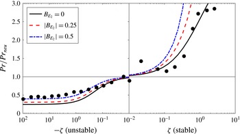
is used. Figure 1 shows the comparison between modelled (lines) and measured (circles)
 $Pr/Pr_{neu}$
as a function of the stability parameter
 $\unicode[STIX]{x1D701}$
in Monin–Obukhov similarity theory (Monin & Obukhov Reference Monin and Obukhov1954).
 $\unicode[STIX]{x1D701}$
is used here instead of
 $R_{f}$
because it is often reported in ASL field experiments.
 $R_{f}$
can be related to
 $\unicode[STIX]{x1D701}$
through
 $R_{f}=\unicode[STIX]{x1D701}/\unicode[STIX]{x1D719}_{m}$
, where
 $\unicode[STIX]{x1D719}_{m}=\unicode[STIX]{x1D705}zS/(-\unicode[STIX]{x1D70F}_{13})^{1/2}$
is the normalized longitudinal velocity gradient for which the Businger–Dyer relation is used (Businger et al.
Reference Businger, Wyngaard, Izumi and Bradley1971; Högström Reference Högström1988),
 $\unicode[STIX]{x1D705}$
is the von Kármán constant and
 $z$
is the height from the ground. It is clear that the model captures the general trend of SGS Prandtl number reported in recent field experiments (Bou-Zeid et al.
Reference Bou-Zeid, Vercauteren, Parlange and Meneveau2008, Reference Bou-Zeid, Higgins, Huwald, Parlange and Meneveau2010). Each circle here is the median value of measured
 $Pr$
over a small range of
 $\unicode[STIX]{x1D701}$
. The model with
 $B_{E_{2}}=0$
better captures the trend under stable conditions while
 $|B_{E_{2}}|=0.5$
(i.e.
 $B_{E_{2}}=-0.5$
when
 $\unicode[STIX]{x1D701}<0$
) better captures the trend under unstable conditions, suggesting that the flux transfer term, which gives rise to
 $B_{E_{2}}$
, is more significant under unstable conditions. This is consistent with many previous studies underscoring the increasingly important role of the flux transport term in the physical domain as the atmosphere becomes more unstable (Stull Reference Stull1988).
Comparison between modelled (lines) and measured (circles)
 $Pr/Pr_{neu}$
as a function of the stability parameter
 $\unicode[STIX]{x1D701}$
. Observational data are taken from field experiments over a lake (Bou-Zeid et al.
Reference Bou-Zeid, Vercauteren, Parlange and Meneveau2008) and a glacier (Bou-Zeid et al.
Reference Bou-Zeid, Higgins, Huwald, Parlange and Meneveau2010).

Second, the sensitivity of
 $Pr$
to the filter scale (
 $\unicode[STIX]{x1D6E5}$
) is investigated. Unlike figure 1 where only one input parameter (
 $B_{E2}$
) was required, the model now needs two input parameters (
 $A_{E_{2}}$
and
 $A_{T}/A_{TT}$
). These two need to satisfy
 $A_{E_{2}}\unicode[STIX]{x1D701}>0$
and
 $A_{T}/A_{TT}>2/3$
. It can be shown that the co-spectral budget model always yields a decreasing
 $Pr$
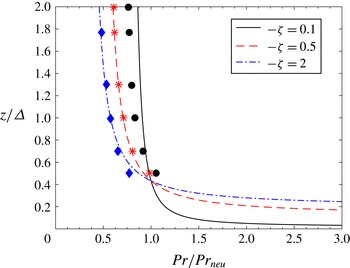
as the filter scale becomes smaller under both stable and unstable conditions. Figure 2 shows three examples under unstable conditions with field experimental data from Vercauteren et al. (Reference Vercauteren, Bou-Zeid, Parlange, Lemmin, Huwald, Selker and Meneveau2008). One can see that both the model and data indicate that the SGS Prandtl number decreases as the filter scale decreases (i.e. as
 $z/\unicode[STIX]{x1D6E5}$
increases), which is also consistent with other experimental studies (Porté-Agel et al.
Reference Porté-Agel, Parlange, Meneveau and Eichinger2001) and the results of dynamic models (Basu & Porté-Agel Reference Basu and Porté-Agel2006). Note that the observational data were averaged over three stability regimes (
 $0<-\unicode[STIX]{x1D701}<0.1$
,
 $0.1<-\unicode[STIX]{x1D701}<1$
,
 $1<-\unicode[STIX]{x1D701}$
) and thus three predictions with different stability parameters are shown in figure 2. It should be also pointed out that
 $\unicode[STIX]{x1D6E5}$
used in the analysis of observational data might not always be in the inertial subrange. Here
 $A_{E_{2}}=-2.7$
and
 $A_{T}/A_{TT}=1.08$
are used in the model but it is not the purpose of this study to calibrate these two parameters using experimental data. Rather the goal here is to study the behaviour of the co-spectral budget model.
Comparison between modelled (lines) and measured (symbols)
 $Pr/Pr_{neu}$
as a function of
 $z/\unicode[STIX]{x1D6E5}$
for three stability regimes.
 $A_{E_{2}}=-2.7$
and
 $A_{T}/A_{TT}=1.08$
are used in the model. Observational data are taken from field experiments over a lake (Vercauteren et al.
Reference Vercauteren, Bou-Zeid, Parlange, Lemmin, Huwald, Selker and Meneveau2008).

The above results focus on the SGS Prandtl number normalized by its neutral value. Here the neutral value of SGS Prandtl number (
 $Pr_{neu}$
) is examined. As already mentioned, earlier theoretical work obtained a value of about 0.47 as the ratio of the Obukhov–Corrsin constant and the Kolmogorov constant for TKE (Schumann et al.
Reference Schumann, Grötzbach, Kleiser and Kollmann1980; Moeng & Wyngaard Reference Moeng and Wyngaard1988; Mason Reference Mason1989). However, there is no consensus on the exact value of
 $Pr_{neu}$
. For example,
 $1/3$
was used by Deardorff (Reference Deardorff1973, Reference Deardorff1980). In addition, the variability of
 $Pr_{neu}$
remains very large in experimental data (Pitsch & Steiner Reference Pitsch and Steiner2000; Porté-Agel et al.
Reference Porté-Agel, Parlange, Meneveau and Eichinger2001; Bou-Zeid et al.
Reference Bou-Zeid, Vercauteren, Parlange and Meneveau2008, Reference Bou-Zeid, Higgins, Huwald, Parlange and Meneveau2010; Vercauteren et al.
Reference Vercauteren, Bou-Zeid, Parlange, Lemmin, Huwald, Selker and Meneveau2008). It can be seen from equation (2.25) that
 $Pr_{neu}$
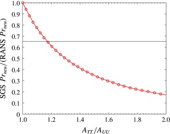
from the co-spectral budget model is dependent on the dissimilarity between momentum and heat in the pressure decorrelation and flux transfer terms. Figure 3 shows the SGS
 $Pr_{neu}$
normalized by its counterpart for RANS modelling when
 $A_{U}/A_{T}=1$
and
 $(1-C_{IU})/(1-C_{IT})=1$
(that is, assuming similarity between momentum and heat in the Rotta model for pressure decorrelation terms). Note that the turbulent Prandtl number for RANS modelling has been previously studied using a similar co-spectral budget model (Katul et al.
Reference Katul, Porporato, Shah and Bou-Zeid2014; Li et al.
Reference Li, Katul and Bou-Zeid2015a
,Reference Li, Katul and Zilitinkevich
b
). It is clear that the value of
 $A_{TT}/A_{UU}$
, which indicates the momentum–heat dissimilarity in the flux transfer term, has a significant impact on the SGS
 $Pr_{neu}$
. The SGS
 $Pr_{neu}$
is only equal to its counterpart in RANS when
 $A_{TT}/A_{UU}=1$
, and the ratio of the two decreases as
 $A_{TT}/A_{UU}$
increases. Typical values used in the literature (i.e.
 $Pr_{neu}=0.47$
and 0.72 for SGS and RANS modelling, respectively) indicate that
 $A_{TT}/A_{UU}\approx 1.18$
, that is, a stronger spectral transfer coefficient for heat than momentum.
The neutral value of SGS Prandtl number normalized by the neutral value of Reynolds-averaged turbulent Prandtl number as a function of
 $A_{TT}/A_{UU}$
. The black line denotes a ratio of
 $0.47/0.72$
.

4 Conclusions and discussion
The subgrid-scale Prandtl number (
 $Pr$
), which is an important parameter in LES, is revisited by solving the co-spectral budgets of momentum and heat fluxes. The co-spectral budget model assumes that the inertial subrange ‘
 $-5/3$
’ scaling applies for
 $k>k_{\unicode[STIX]{x1D6E5}}$
(the wavenumber corresponding to the filter scale
 $\unicode[STIX]{x1D6E5}$
), as compared to prior models that assume that the ‘
 $-5/3$
’ scaling applies for
 $0<k<k_{\unicode[STIX]{x1D6E5}}$
. The model also invokes the Rotta model for parameterizing the pressure decorrelation term and a gradient diffusion model for parameterizing the flux transfer term. The resulting
 $Pr$
is stability- and scale-dependent, which is contrary to prior
 $Pr$
estimates that are stability-independent and scale-invariant. More specifically,
 $Pr$
increases (decreases) as the atmosphere becomes stable (unstable) and decreases as the filter scale becomes smaller, which is in good agreement with field experimental data and the results of dynamic models.
The influence of stability on
 $Pr$
comes from the dependence of
 $Pr$
on the resolved longitudinal velocity and temperature gradients, which are strongly affected by thermal stratification. In this study, the resolved longitudinal velocity and temperature gradients are ‘imposed’ on the SGS flow. This assumption is often made for SGS (and RANS) modelling to simplify the analysis but may not always be realistic, especially for more complex turbulent flows. The trend of
 $Pr$
with stability suggests that buoyancy production (destruction) of TKE enhances (reduces) the turbulent transport efficiency of heat compared to momentum (Li & Bou-Zeid Reference Li and Bou-Zeid2011; Li, Katul & Bou-Zeid Reference Li, Katul and Bou-Zeid2012) even at subgrid scales.
On the other hand, the dependence of
 $Pr$
on the filter scale, even when the filter scale is within the inertial subrange, stems from the fact that the co-spectra of momentum and heat fluxes have different scaling laws, which is further caused by the dissimilarity between the scale-wise transfer of momentum and heat and their interactions with pressure fluctuations. Unlike the energy spectra, which have a well-established ‘
 $-5/3$
’ scaling in the inertial subrange, the flux co-spectra seem to show non-universal behaviours (Bos et al.
Reference Bos, Touil, Shao and Bertogli2004, Reference Bos, Touil and Bertoglio2005; Bos & Bertoglio Reference Bos and Bertoglio2007). The neutral value of
 $Pr$
is also dependent on the momentum–heat dissimilarity in the Rotta model and the gradient diffusion model. If Reynolds analogy is assumed in the Rotta model, the fact that under neutral conditions the SGS Prandtl number is smaller than the Reynolds-averaged turbulent Prandtl number is an indication of a stronger spectral transfer coefficient for heat than for momentum.
The model (2.27) proposed here can be readily implemented and is mainly dependent on three well-established phenomenological constants (i.e. the Kolmogorov constant for the vertical velocity variance, the Obukhov–Corrsin constant and the isotropization constant in the Rotta model). Even for dynamic models, this parameterization for
 $Pr$
can avoid a dynamic determination of SGS heat diffusivity. To account for the stability effect,
 $B_{E_{2}}=0$
and
 $B_{E_{2}}=-0.5$
are recommended for stable and unstable conditions, respectively. The model can also account for the scale dependence given the values of
 $A_{E_{2}}$
and
 $A_{T}/A_{TT}$
, which need further investigations. The exact value of
 $Pr$
under neutral conditions also remains an open question.
Although the model is developed and validated in the atmospheric surface layer, it may be applied to more general conditions (at least as a first-order correction to prior models) if the Reynolds number is sufficiently large and the filter scale is within the inertial subrange (but not too close to the Kolmogorov scale) so that most assumptions made here remain valid. A useful extension of this work would be to compare the performance of the co-spectral budget model to prior models and empirical parameterizations (Brown et al. Reference Brown, Derbyshire and Mason1994; Mason & Brown Reference Mason and Brown1999) for simulation of stratified turbulent flows.
Acknowledgements
The author thanks Professor E. Bou-Zeid from Princeton University for providing the observational data used in figure 1 and for inspiring discussions. Comments and suggestions from the two reviewers are greatly appreciated.