NOMENCLATURE
 $E_0,H$
internal energy, enthalpy [
${\rm J/m}^3$]- f
volumetric force [
${\rm N/m}^3$]- $\overline{f}$
body-force terms vector [-]
- I
shaft inertia [
${\rm kg} \cdot {\rm m}^2$]- i
incidence angle [deg]
- M
Mach number [-]
- $\dot{m}, \dot{m}'$
mass flow [kg/s], design point normalised corrected mass flow [-]
- P
pressure [Pa]
- PR
pressure ratio [-]
- r
radius [m]
- Re
Reynolds number [-]
- $\overline{S}$
source terms vector [-]
- T
temperature [T]
- $t, \mathrm{d}t$
time, time step [s]
- $\overline{U}$
conservative variables [-]
- u
flow velocity [m/s]
- x
axial position [m]
- $W_{\rm EX}$
work exchange [
${\rm W/m}^3$]


Greek symbols
- $\beta$
angle in the streamline direction [deg]
- $\gamma$
stagger angle [deg]
- $\delta$
deviation angle [deg]
- $\theta$
circumferential position [rad]
- $\rho$
density [
${\rm kg/m}^3$]- $\sigma$
solidity [-]
- $\tau$
torque [
${\rm N} \cdot {\rm m}$]- $\tau'$
corrected torque parameter [
${\rm N} \cdot {\rm m/Pa}$]- $\Omega, \Omega'$
rotational speed [rad/s], normalised rotational speed [-]
- $\omega$
pressure loss coefficient [-]


Subscripts
- $r,x,\theta$
radial, axial, circumferential direction
- METAL
direction of the metal camber line
- FLOW
direction of the flow
- IN
blade row inlet conditions
- OUT
blade row outlet conditions
- T
total quantity

1.0 INTRODUCTION
Aviation engines are exposed to the sub-idle regime on start-up or during windmill relight. While these events have historically not warranted a detailed performance evaluation, more stringent certification standards, customer requirements and the push for marginal benefits in fuel efficiency have highlighted the need for accurate sub-idle performance characterisation(1). Additionally, modern engines with increasing by-pass ratios put a strain on relight capability, while larger gearboxes and driven accessories also contribute to increased windmilling drag and reduced starting performance(Reference Zachos2). As the trend towards higher by-pass ratios and geared configurations continues, so too does the need for improved sub-idle performance, requiring improved prediction techniques.
The sub-idle portion of a map can be divided into three distinct regions depending on the sign of the work and total pressure changes, as shown in Fig. 1. While any point with a pressure ratio above unity is considered to lie within the compressor operation region, the regions with a total pressure loss can be divided into stirrer and turbine modes depending on the sign of the work input. In the stirrer mode, there is a work addition to the flow along with a pressure loss, while work extraction and pressure loss define the turbine mode. A key element of the map is the boundary between these last two regions, which corresponds to the torque-free windmilling characteristic in which there is no net torque on the shaft and no net work done on the gas. In the absence of loads and frictional losses, the torque-free windmilling line could be reached by a compressor simply due to the incoming flow, and represents the maximum speed attainable by an unpowered compressor at a given mass flow. In a real-life application, the presence of a turbine can result in steady-state windmilling operation above the torque-free windmilling line. Conversely, frictional losses and work extraction would bring the operational point into the turbine region(Reference Walsh and Fletcher3). At the lower extreme of the map, the locked-rotor line corresponds to zero-speed operation, where flow simply passes through the compressor, incurring a pressure loss and imparting torque on the shaft. Because the net enthalpy change ( $\Delta H$
) becomes zero at the torque-free windmilling and locked-rotor lines of an adiabatic compressor, performance parameters containing an enthalpy term in the denominator are not continuously defined throughout the sub-idle region. For this reason, the corrected torque parameter (
 $\tau'$
) is used alongside the pressure ratio and corrected mass flow to describe compressor performance in the sub-idle region(Reference Riegler, Bauer and Kurzke4). This parameter is defined as the shaft torque divided by the inlet total pressure(Reference Walsh and Fletcher3).
Example of sub-idle compressor map with different operating regimes.

In order to accurately predict whole-engine performance using a synthesis solver, maps for the different engine components are required. As data on performance at speeds lower than the idle conditions are scarce and not generally obtained from rig tests, a way to generate these maps must be devised. Several techniques have been proposed for the generation of sub-idle compressor maps using a variety of graphical(Reference Kurzke5) or analytical methods(Reference Agrawal and Yunis6,Reference Gaudet and Gauthier7) . However, these are generally low-fidelity approximations that limit the accuracy of the generated performance data. A review of these methods can be found in Jones et al(Reference Jones, Pilidis and Curnock8). Previous work at Cranfield University has looked at enhancing map generation by including interpolation from limited sub-idle data, e.g. locked-rotor and windmilling characteristics(Reference Zachos, Ruelke, Pachidis and Singh9,Reference Ferrer-Vidal, Pachidis and Tunstall10) . While these latter methods have been shown to result in viable maps, they highlight the need to accurately calculate the locked rotor and, especially, windmilling characteristics to further improve the reliability of the maps generated. The numerical scheme presented in Righi et al(Reference Righi, Pachidis and KÖnÖzsy11) has shown the capability to model compressor operation in extreme off-design cases, and as such is a strong candidate for application to the sub-idle case. This paper considers the adaptation of the low-order through-flow code presented in that work to the modelling of a modern multi-stage, high-speed, high-pressure compressor in sub-idle conditions along with validation against high-fidelity 3D CFD simulations. The significance of these simulation results is that they may be used as inputs to the map generation method presented in Ferrer-Vidal et al(Reference Ferrer-Vidal, Pachidis and Tunstall10), yielding compressor maps with improved accuracy.
2.0 LOW-ORDER MODELS
2.1 Euler numerical method
The Axial Compressor Rotating Stall and Surge (ACRoSS) code is a through-flow code developed at Cranfield University(Reference Righi, Pachidis and KÖnÖzsy11). The code was originally created to handle compressor stall transients, where a 3D formulation is required for the proper simulation of stall cells. For sub-idle modelling, however, the flow is considered to be axisymmetric and a two-dimensional (2D) formulation is used by setting the number of circumferential elements to one. The flow equations are solved transiently on a relatively coarse grid, as required to maintain acceptable computational cost. A structured mesh is generated based only on the annulus geometry and the input number of elements in the axial, radial and circumferential directions, with no need for detailed mesh generation. The compressor annulus is discretised as an empty duct, and the blade rows are introduced using the body-force method. The equations solved are the unsteady, compressible, cylindrical Euler equations, written in matrix form as
 \begin{align}\frac{\partial}{\partial t}\begin{bmatrix}\rho \\\rho u_r \\\rho u_\theta \\\rho u_x \\\rho E_0\end{bmatrix}&=-\frac{1}{r} \frac{\partial}{\partial r}\begin{bmatrix}\rho r u_r \\\rho r u_r^2 \\\rho r u_\theta u_r \\\rho r u_x u_r \\\rho r H_0 u_r\end{bmatrix}-\frac{1}{r} \frac{\partial}{\partial \theta}\begin{bmatrix}\rho u_\theta \\\rho u_r u_\theta \\\rho u_\theta^2 + P \\\rho u_x u_\theta \\\rho H_0 u_\theta\end{bmatrix}-\frac{\partial}{\partial x}\begin{bmatrix}\rho u_x \\\rho u_r u_x \\\rho u_\theta u_x \\\rho u_x^2 + P \\\rho H_0 u_x\end{bmatrix}\nonumber\\[4pt]
&\quad+\underbrace{\begin{bmatrix}0 \\\frac{\rho u_\theta^2}{r}-\frac{\partial P}{\partial r} \\-\frac{\rho u_\theta u_r}{r} \\0 \\0\end{bmatrix}}_{\overline{S}}+\underbrace{\begin{bmatrix}0 \\f_r \\f_\theta \\f_x \\W_{\rm EX}\end{bmatrix}}_{\overline{f}}\end{align}
where  $\overline{f}$
is the vector of the body-force terms and
 $\overline{S}$
is the source terms vector. The monotone, first-order Godunov scheme is used for the solution of Equation (1), where the time-stepping is performed using an Euler forward scheme.
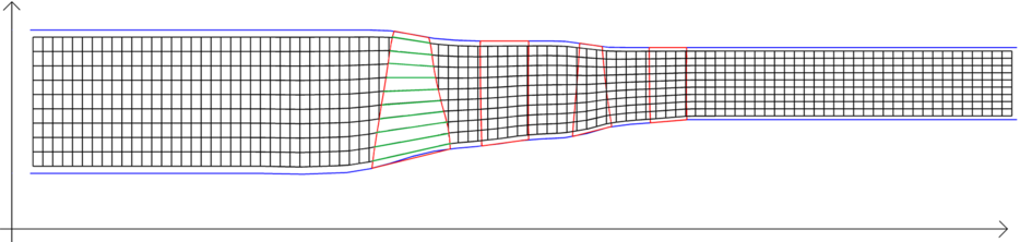
The formulation used to calculate the body forces is derived from those proposed in Longley(Reference Longley12) and Brand(Reference Brand13). The forces are calculated along the pseudo-planes formed by the grid, as shown in Fig. 2. The forces are then decomposed and applied onto the grid in the radial, circumferential and axial directions, represented by  $f_r,f_\theta,f_x$
in the source term of Equation (1). A work exchange term
 $(W_{\rm EX})$
is also included to account for the work input by the rotors to the flow. A detailed explanation of this methodology is given in Righi et al(Reference Righi, Pachidis and KÖnÖzsy11).
Example of the automatically generated grid. Highlighted in green are the pseudo-planes along which the body forces are applied, created by connecting axially the volume centroids.

An external algorithm is necessary to estimate at every iteration the performance of the blade row, expressed as a pressure loss coefficient  $\omega$
and a deviation
 $\delta$
, defined as
 \begin{equation}\omega = \frac{\Delta P_{T}}{0.5\rho u^2} \quad\quad \quad\quad \delta = \beta_{\textrm{{FLOW\:OUT}}}-\beta_{\textrm{{METAL\:OUT}}}\:\end{equation}
These are estimated for every blade row and at every pseudo-plane, based on the blade geometry and the flow conditions at the leading edge (LE) and trailing edge (TE).
A set of empirical correlations taken from literature(Reference Aungier14) and a set developed by Rolls-Royce plc. are implemented in the code to model the performance of the blade during normal operations.
Neither of these sets of correlations is well suited to model separated blade rows, and the performance in such conditions is extrapolated from the normal operation. When separation occurs close to surge margin, it quickly triggers a compressor stall and an accurate prediction of  $\omega$
and
 $\delta$
is not necessary. However, in case of separation due to a highly negative incidence angle i, as occurs during sub-idle conditions, a better prediction is necessary to model the steady, separated flow. In a previous effort, three low-order models for separated passages at negative incidence were tested to model a small multi-stage compressor in sub-idle conditions and the results were compared against experimental data. A set of correlations created by Ferrer-Vidal et al, presented in Ref. (Reference Ferrer-Vidal, Schneider, Allegretti and Pachidis15), was found to be the model with the best accuracy; the results are reported in Section 4.2.
These correlations are implemented here in ACRoSS and used only for negative incidence  $i<0^\circ$
, thus yielding loss and deviation as a function of cascade geometry and inlet conditions:
 \begin{equation}(\omega, \delta)= f(\gamma, \sigma, i, M_{IN})\end{equation}
This new set of correlations is ‘blended’ to the standard set close to  $i=0^\circ$
to avoid sudden jumps in performance.
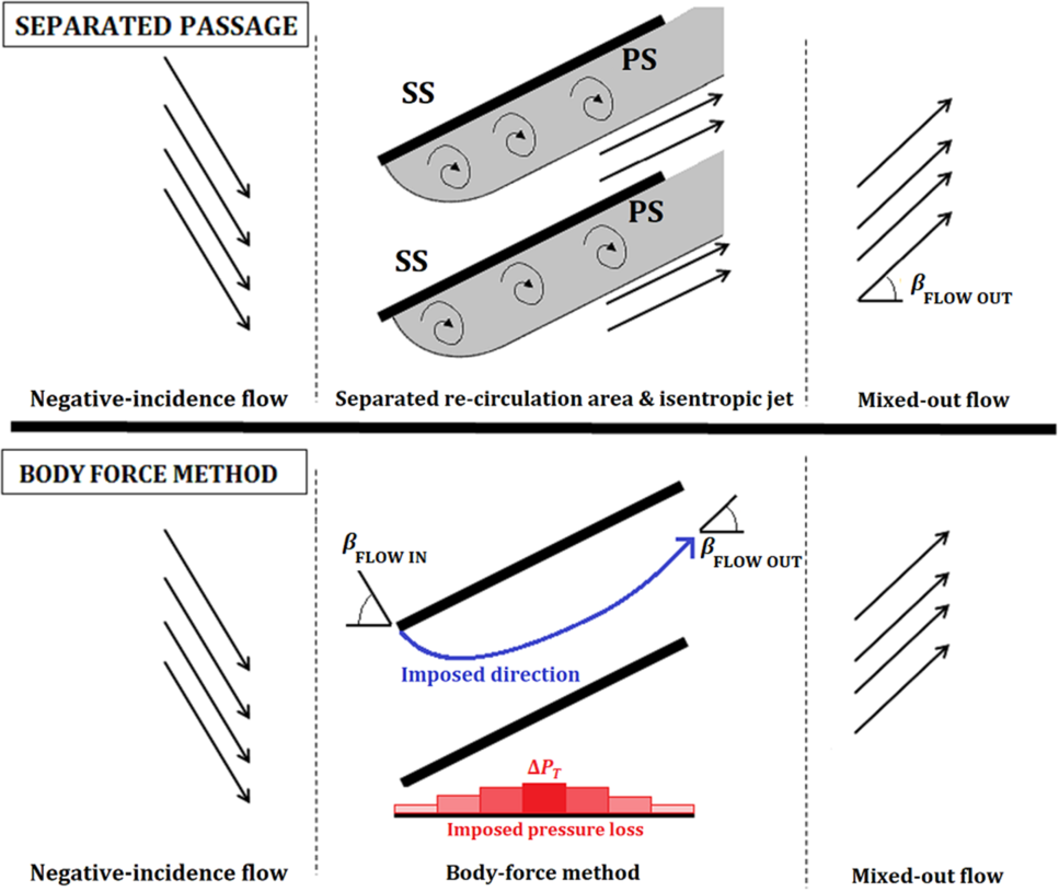
The body-force method imposes the turning and pressure loss on the flow as predicted by the empirical correlations. The body forces also ensure that the flow direction at the TE matches the value predicted by the deviation correlation. The pressure loss  $\Delta P_{T}$
is redistributed in the grid elements inside of the blade row and introduced by means of a force aligned to the flow. This implies that all of the turning and the pressure loss occur inside the blade row while the next blade row will observe a uniform inlet flow.
While this method offers an appropriate representation for unstalled conditions, when flow stalls and separates the physical behaviour can be very different. In the case of a separated passage, a large change in flow direction occurs during mixing downstream of the blade, with the resulting outflow angle being potentially very different from that observed at the TE. Similarly, the separated flow remains mostly isentropic inside the blade passage and the pressure loss occurs mainly during the mixing. In a real compressor, the rows are close enough that typically only part of the mixing will occur between the blades, thus the flow is not uniform at the next row LE.
By introducing the sub-idle model into the low-order tool, we are thus imposing that, even when a passage separates, the uniform, fully mixed conditions (the output of the model) are reached before the next blade LE; the authors refer to this as the fully mixed wake assumption. Figure 3 shows the model of a separated passage blade on which the correlations are based and how it is represented by the body-force model.
Model of a separated blade passage at high negative incidence and its implementation with the body-force method along one of the pseudo-planes at a specific span position.

The assumption introduced has two important implications:
The interaction of the next blade row with the mixing of the wakes is ignored.
The performance of a blade row is estimated using as inlet conditions the uniform representation of the flow, and not the real separated flow.
As the flow is expected to be largely separated at the high negative incidences which occur in sub-idle conditions, the validity of this assumptions needs to be independently investigated.
To model the locked-rotor case, the shaft RPM is set to zero. For the windmilling case, the torque on the rotors is calculated at every iteration and a simple balance equation is used to alter the rotational speed as shown in Equation (4). The rotational speed changes until the torque matches the target value  $\tau_{\rm target}$
, set to zero for the torque-free windmilling case. For the windmilling case, ACRoSS is employed in a pseudo-transient approach, so the shaft inertia I is set to a very low value to accelerate convergence.
 \begin{equation}\Omega^{t+1}=\Omega^t+\frac{\sum \tau + \tau_{\rm target} }{I} \cdot \mathrm{d}t\end{equation}
Non-reflecting boundary conditions are applied at the inlet and outlet of the model(Reference Poinsot and Lele16); total quantities are imposed at the flow inlet, and static pressure is imposed at the outlet. To generate the characteristics, the outlet static pressure is lowered incrementally to simulate throttling.
2.2 Mean-line approach
The mean-line tool employs the well-known mean line, or pitch line, approach to solve the velocity triangles blade-by-blade from knowledge of the compressor mean-line geometry. Such an approach requires knowledge of the blade deviation angles and loss coefficients to calculate the blade outlet conditions through the compressor. The same negative incidence loss and deflection model used for the Euler body-force method has been used here(Reference Ferrer-Vidal, Schneider, Allegretti and Pachidis15). Like in the Euler method, the mean-line approach’s mono-dimensional implementation necessarily implies fully mixed wakes by assuming that all losses have been realised by the time the flow reaches the subsequent blade row. Continuity is conserved through the solution of the axial velocity at the entry to the blade passage, while momentum conservation is also established through the solution of the axial pressure distribution. Changes in the pitch line radius and flow path area are taken into account through conservation of angular momentum. The calculation is however one-dimensional, as only the pitch line geometry is considered. The mean line approach is an established method, and no further details are given here. Good overviews of the method may be found in Refs (Reference Veres17) and (Reference Smith18).
A point to note regarding the mean-line approach for the sub-idle regimes is the selection of the mean radius. In sub-idle conditions, the span-wise work distribution may vary drastically along the span. This is particularly true for single-stage fans, where part of the fan expands the flow while the other compresses it(Reference Binder, Courty-Audren, Duplaa, Dufour and Carbonneau19). In such a case, the selection of a single radial location to characterise performance can yield misleading results. For multi-stage machines with high hub-to-tip ratio, this change in operation occurs primarily with axial rather than radial location. Typically, the front stages compress the flow, the rear stages expand it and an intermediate blade row acts as the switch-over point between the regimes; this is observed in the case analysed and presented in Section 4.3. The selection of a radius to characterise the performance of multi-stage core compressors is therefore not as critical as for fans. In this work, the mean radius used for analysis is just the mean geometric radius between the hub and shroud.
3.0 RANS NUMERICAL METHODS
The compressors studied have been modelled using 3D RANS CFD simulations as a verification of the low-order approach. Two-dimensional (2D) RANS CFD cascade models have also been used to independently investigate the adequacy of the fully mixed wake assumption.
3.1 3D compressor models
The 3D CFD models are generated from geometry provided by Rolls-Royce plc. The geometry is discretised with a structured mesh generated using the ANSYS® TurbogridTM software. The models consist of the clean blade geometry with no bleeds or leaks taken into account. In all cases, a wall-modelled mesh is used with  $y+= \sim30$
. The mesh size is 5
 $\sim$
6
 $\times 10^5$
elements per blade passage. With the sole goal of obtaining pressure ratio and torque values, a mesh sensitivity study was performed on a single-stage simulation at locked-rotor conditions. The error between the employed grid and the finest considered (at 8
 $\times 10^6$
elements per passage) was negligible for pressure ratio and 0.7% for torque. Simulations are run with the ANSYS® CFX® solver, release 18.2, using a
 $k-\omega$
shear stress transport (SST) turbulence model and employing the automatic wall-function treatment. Boundary conditions consist of the inlet total pressure and temperature and mass flow at the outlet. The inlet conditions used are 1 atm and 288.15K. No-slip walls are used on blade and hub surfaces. The casing over the rotor tips is a stationary no-slip wall in the absolute reference frame (counter-rotating wall). Tip gaps are modelled for rotor blades as 1
 $\%$
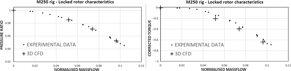
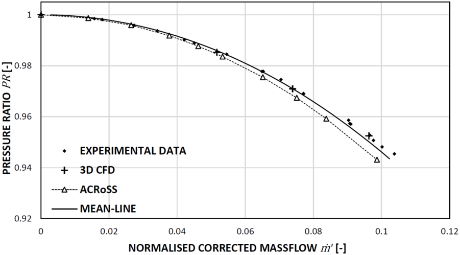
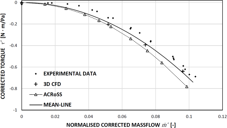
of the span and discretised with 15 elements. The multi-stage compressors are modelled using mixing planes between each blade row, such that the flow field is averaged before passing onto the next blade row. This allows a single-passage model to be used. While the large separated wakes present at locked-rotor conditions would span several passages, forgoing the use of mixing planes requires domain pitches to be matched, which in the case of a modern multi-stage compressor, entails the modelling of large annular sectors, straining computational resources. Since the goal of this investigation is to compare 3D Navier–Stokes CFD results against low-order models which also employ the blade row mixing assumption, this limitation in the numerical model is deemed acceptable for the analysis. The fully mixed wake assumption is discussed in detail below. The known limitations of steady RANS CFD simulations to accurately capture the physics of separated flows needs to be considered when attempting to apply these methods to sub-idle operation. However, as the current application seeks to develop methods that predict bulk performance parameters, the emphasis must be put on using RANS CFD as the highest-fidelity through-flow tool available, used solely to calculate characteristics. A previous study(Reference Righi, Ferrer-Vidal, Allegretti and Pachidis20) already compared CFD results against experimental data with a favourable outcome, as can be seen in Fig. 4.
Locked rotor pressure ratio and corrected torque characteristics as measured in experiment and calculated in CFD. Adapted from Ref. (Reference Righi, Ferrer-Vidal, Allegretti and Pachidis20).

Reduced-order models that are at least able to match the performance of RANS CFD while offering significant reductions in overhead and computational requirements are important to engineers in need of fast and reliable performance data.
3.2 2D cascade study
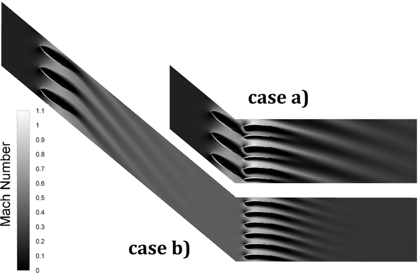
The validity of the fully mixed wake assumption is assessed using a 2D CFD RANS model consisting of two blade rows subjected to a high negative incidence flow. The model is solved using the ANSYS® Fluent® solver, release 18.2. The CFD implementation is purely 2D (no geometry or mesh extrusion), resulting in unity axial–velocity density ratio. Six studies are performed with different sets of blade rows. For each study, we distinguish a case (a) with the rows at short distance (1 chord), and a case (b) with rows far apart ( $\sim$
6 chords) such that the separation wakes from the first row are fully mixed out before reaching the second; an example is presented in Fig. 5.
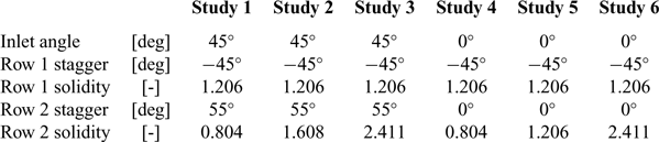
The first blade row has constant stagger and solidity but two different settings of inlet angle, so that two magnitudes of wakes can be studied. The solidity of the downstream blades changes in every study, so that the interaction of wakes and passages changes every time. The details of the studies are reported in Table 1.
Set-up of the CFD studies used to assess the fully mixed wake assumption

Example of CFD simulations using ANSYS® Fluent® software of separated blade rows with normal inter-blade distance, case (a), and large distance, case (b).

All blade rows consist of the same mid-stage rotor profile which was used in the CFD campaign from which the negative incidence loss and deviation models were developed(Reference Ferrer-Vidal, Schneider, Allegretti and Pachidis15). All simulations are run with stationary blade rows. The equations solved are the compressible RANS; the turbulence is modelled using the k– $\omega$
SST model. Total pressure and temperature are prescribed at the inlet; static pressure at the outlet is set to obtain the specified target mass flow. For every study and case, the mesh was checked for grid convergence. The finest grid used on the largest domain, case (b) study 3, has
 ${\sim}1.25 \times 10^6$
elements.
4.0 RESULTS AND DISCUSSION
The fully mixed wake assumption is considered first, followed by a discussion of the application of the low-order models to two specific multi-stage compressor geometries.
4.1 Fully mixed wake assumption
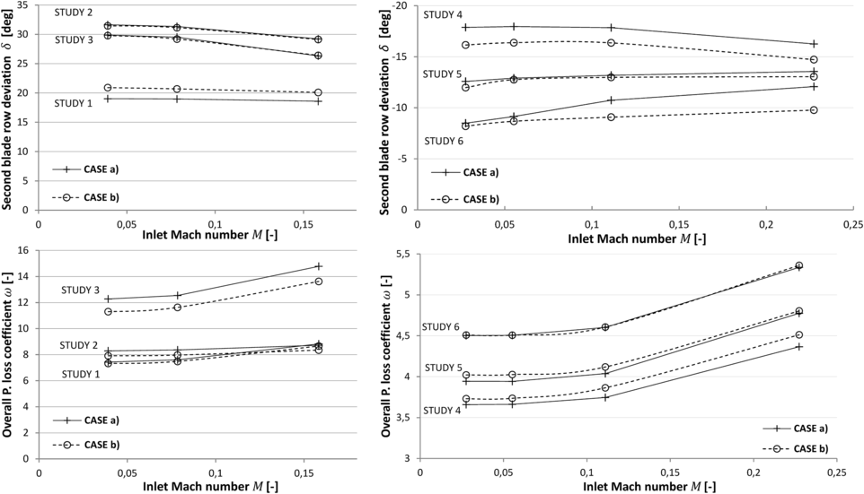
Using the 2D cascade model developed, pressure loss and deviation values obtained with different levels of inter-blade mixing can be compared. These are estimated using the flow at domain inlet and domain outlet. The domain extends several chords downstream of the second blade row. In all studies, the wake mixes fully within the domain and the flow is uniform by the time it reaches the outlet, where it is measured. The results are presented in Fig. 6. The pressure loss is reported using an overall pressure loss coefficient, defined as the total pressure difference between domain inlet and outlet normalised over the dynamic head at domain inlet. The deviation angle reported is calculated on the last blade row, using the mixed-out flow direction at domain outlet. The Reynolds number in the study varies from  $2\times 10^4$
at low Mach number to
 $2\times 10^5$
at maximum Mach number.
Results from the 2D cascade CFD simulations. Overall pressure loss coefficient and deviation angle are compared from six different set-ups with normal inter-blade distance, case (a), and large distance, case (b).

From the results, it can be observed that, in every study, the difference in the deviation angle is less than 2.5 $^\circ$
between the two cases. The discrepancy in pressure loss coefficient is up to
 $\sim$
8%. It should be noted that, as the discrepancy reported is in pressure loss and not pressure ratio, it does not multiply along the blade rows, and in a multi-stage compressor the cumulative error in pressure loss coefficient would not be higher than the maximum error of the individual rows.
Based on these results, the fully mixed assumption is considered accurate enough for the fast creation of windmilling and locked-rotor characteristics.
4.2. Six-stage turbo-shaft compressor
In this study, a six-stage turbo-shaft compressor is modelled using the mean-line tool and the ACRoSS code in windmilling and locked-rotor conditions. The results are compared with 3D RANS CFD and experimental data from Ref. (Reference Righi, Ferrer-Vidal, Allegretti and Pachidis20).
For pressure ratio in the locked-rotor case (Fig. 7), all models match well, with discrepancies from experimental data well below 1%. For the torque however (Fig. 8), the matching is more moderate. The maximum discrepancies in torque reach 20%, although such a large relative discrepancy is simply due to the low torque values considered. The maximum absolute torque discrepancy is  $0.15{\rm N} \cdot {\rm m}$
.
Comparison of the six-stage turbo-shaft locked-rotor pressure ratio characteristics calculated using 3D CFD and the two low-order models, compared with experimental data from Ref. (Reference Righi, Ferrer-Vidal, Allegretti and Pachidis20).

Comparison of the six-stage turbo-shaft locked-rotor torque characteristics calculated using 3D CFD and the two low-order models, compared with experimental data from Ref. (Reference Righi, Ferrer-Vidal, Allegretti and Pachidis20).

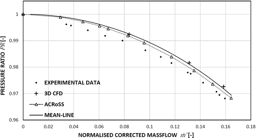
All models including CFD appear to under-predict pressure losses in the torque-free windmilling case, as seen in Fig. 9. The two low-order models match the experimental data more accurately in this case, with the maximum discrepancy between the mean-line method and experiment being  $0.3\%$
.
Comparison of the six-stage turbo-shaft torque-free windmilling pressure ratio characteristics calculated using 3D CFD and the two low-order models, compared with experimental data from Ref. (Reference Righi, Ferrer-Vidal, Allegretti and Pachidis20).

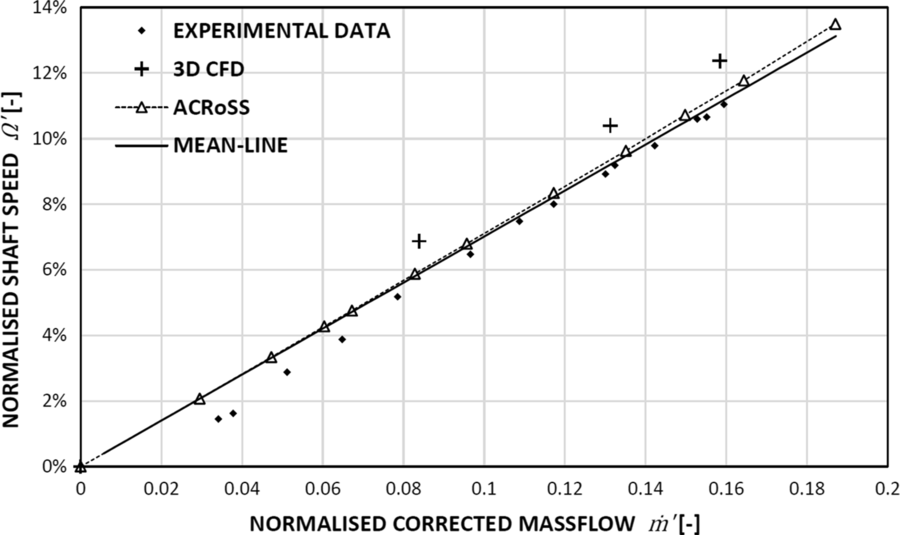
For torque-free windmilling, the net shaft torque is taken as zero and the value worth comparing is the predicted RPM obtained from the low-order models. For the RANS solutions, an iterative approach was taken to vary the outlet boundary condition until torque was zeroed. Figure 10 shows the resulting level of matching for the different models, with the low-order approaches again out-performing the RANS results in this specific case, with a discrepancy in the predicted slope of only  $1.3\%$
for ACRoSS compared with
 $3.1\%$
for the RANS CFD. The improved performance of the low-order models can partly be attributed to the iterative approach used in reaching a zero-torque condition. Iterative variation of the boundary conditions with RANS CFD can only reach torque levels below
 $1{\rm N} \cdot {\rm m}$
before computational time becomes excessive, while two orders of magnitude tighter convergence can be reached with the two low-order models.
Comparison of the six-stage turbo-shaft torque-free windmilling speeds calculated using 3D CFD and the two low-order models, compared with experimental data from Ref. (Reference Righi, Ferrer-Vidal, Allegretti and Pachidis20).

4.3 Six-stage high-pressure compressor
The previous geometry was chosen due to the availability of experimental data, but it is not representative of modern large civil engines. Additionally, the previous test case did not include data at very high mass flows, so the applicability of the methods to conditions near choke could not be readily evaluated. In order to apply the methods to a more relevant case, a six-stage high-speed high-pressure compressor (HPC) representative of modern aero-engines is also investigated and calculations from the mean-line and ACRoSS models are compared with the 3D RANS CFD simulations. As no experimental data are available for this compressor, RANS CFD is taken as the reference, considered here as the conceptually highest-fidelity tool available.
The ACRoSS model has a grid of 920 axial  $ \times\:12$
radial elements, the annulus duct is extended straight in front and behind the blade rows by
 $\sim$
1 front-stage blade chord. This very short domain speeds up the calculation and is acceptable in this application as no mixing is expected in front of or behind the compressor. The results of some selected cases have been also reproduced with longer inlet and outlet ducts, to ensure that no error is introduced by the shortened domain. A convergence study was also performed to check that grid independence is reached.
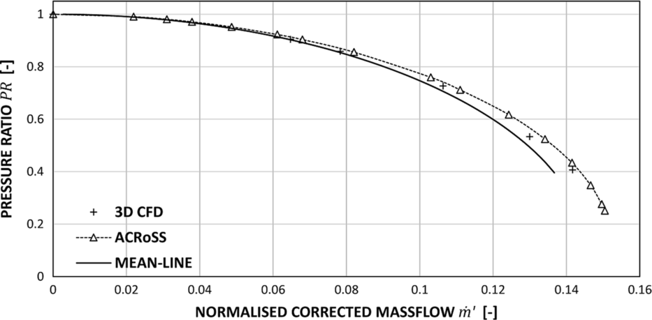
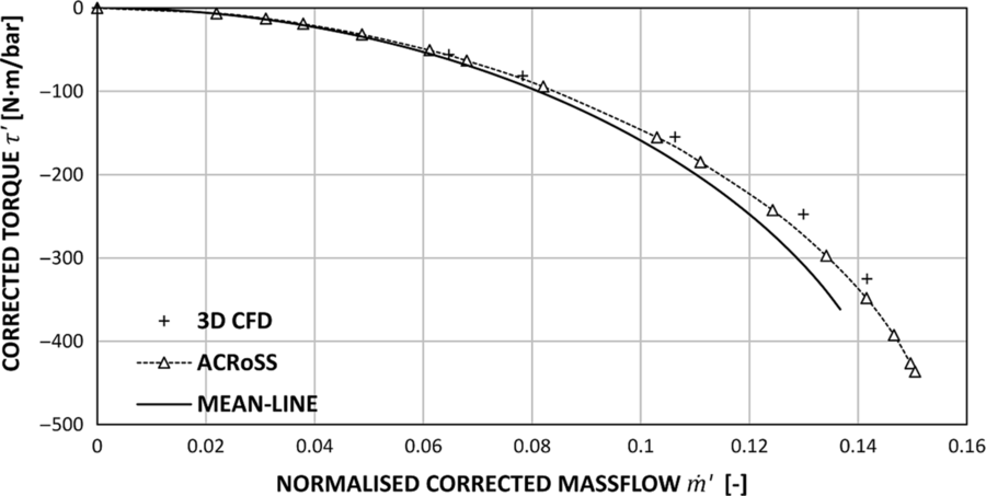
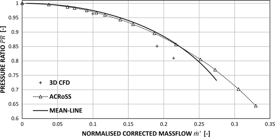
The results for the locked-rotor conditions are presented in Figs 11-12. The characteristics are presented using the corrected mass flow normalised over the design value,  $\dot{m}'$
, total-to-total pressure ratio, PR, normalised shaft speed,
 $\Omega'$
, and the corrected torque parameter,
 $\tau'$
, defined as the torque on the shaft divided by the inlet total pressure. As the present study focuses on sub-idle conditions, these are expected to be much lower than the design value (set at 100% speed). The characteristic created using ACRoSS extends until choking conditions are reached at
 $\dot{m}'=0.15$
. The choking occurs as the flow reaches sonic conditions inside a blade row. This is not accurately modelled by the body-force method, because the blade thickness and the separation in the passages are not taken into account by the Euler solver. However, as the flow approaches choking conditions, the rapid increase of the pressure loss coefficient causes the characteristic to steepen, and choking mass flow is quickly reached.
Comparison of the six-stage HPC locked-rotor pressure characteristic predictions using high-fidelity 3D CFD and the two low-order models.

Comparison of the six-stage HPC locked-rotor torque characteristic predictions using high-fidelity 3D CFD and the two low-order models.

The mean-line analysis matches very closely the data from CFD along the whole characteristic. The ACRoSS code gives better results compared with the mean-line tool, as the latter over-predicts the pressure losses close to choking conditions.
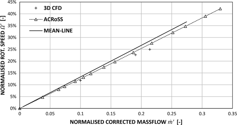
The comparison of the results for windmilling conditions are presented in Figs 13-14. The windmilling signature is reported using the corrected rotational speed normalised by the design value  $\Omega'$
. In the current study, all results are obtained through numerical models in which friction is not included; as a result, the data in Fig. 14 align with the origin of the chart.
Comparison of the six-stage HPC windmilling pressure characteristic predictions using high-fidelity 3D CFD and the two low-order models.

Comparison of the six-stage HPC windmilling signature line predictions using high-fidelity 3D CFD and the two low-order models

Both low-order tools under-predict the pressure losses with respect to the CFD results; as observed in the locked-rotor simulation, the characteristics from the low-order tools diverge close to choking conditions, with the mean-line tool predicting higher pressure losses. Despite the large difference in the pressure characteristics, the signature line is closely reproduced and the discrepancy from CFD data in the line slope is 7.5% for ACRoSS and 12% for the mean-line tool.
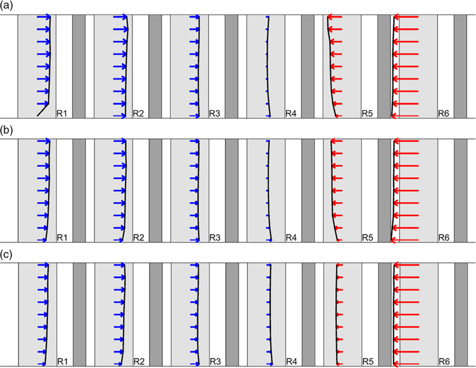
Because of its span-wise resolution, the ACRoSS code can analyse the different torque contributions that blade rows make at different radial positions during windmilling, potentially identifying blades which act both as a compressor and as a turbine. However, the results from ACRoSS show that, for this multi-stage high hub-to-tip ratio machine, the radial distribution of torque is mostly uniform, as shown in Fig. 15, with only some small variations seen at lower speeds. These results justify the use of the mean geometric radius as reference radius in the mean-line code for this type of compressor (i.e. core multi-stage compressors with high hub-to-tip ratio). As previously described by Righi et al(Reference Righi, Ferrer-Vidal, Allegretti and Pachidis20), the axial distribution of torque remains mostly constant at different speeds in windmilling conditions.
Rotor torque distribution in windmilling conditions at different speeds, (a) 5%  $\Omega'$, (b) 19%
 $\Omega'$, (c) 32%
 $\Omega'$. Values not to scale across speeds. Blade rows acting as compressors are presented in blue, and rows acting as turbines are in red.

By analysing the flow field, it was observed that, at rotor 1 hub (and, at higher speed, also rotor 2), the blade is highly loaded, resulting in a stall with positive incidence being predicted by ACRoSS. This yields a large deviation and reduced mass flow and torque locally at the rotor 1 hub, as seen in Fig. 15. Because of the rotor mismatching, the stators in the front stage remain at a high negative incidence angle at the tip. This causes the flow to separate, causing a local increase in deviation. Away from these stalled areas, deviation and pressure loss remain mostly constant or linear in the span-wise direction in all blade rows. The alignment of the characteristics from ACRoSS and the mean-line code indicates that the locally stalled areas have a very limited effect on the overall performance. Radial redistribution of the flow is found to be negligible for these simulations. At all speeds, the flow in the meridional plane is misaligned from the pseudo-planes (and in general from the grid) by less than  $5^{\circ}$
throughout.
4.4 Computational cost
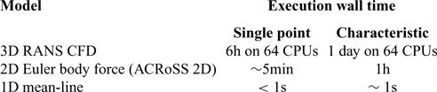
The accuracy of the prediction of the sub-idle characteristics must be considered with the associated computational cost to assess the trade-off. Table 2 presents the computational times required to model a single operating point and a characteristic. Each code has been run using the computational resources which would typically be expected. The mean-line tool and ACRoSS have been run on a single quad-core workstation; ACRoSS is a parallel code, and only one instance of the program is run at a time, requiring all the cores. The 3D CFD model has been run in parallel on a HPC facility, using 64 CPUs distributed across four nodes with MPI and InfiniBand interconnect.
Computational cost of the different models considered

Based on these computational costs, the different methods seem to be appropriate for different applications:
The mean-line method gives the least knowledge of the flow field and has the most discrepancy from RANS CFD near the choke, but it is the only method fast enough to be automated for creation of characteristics or optimisation.
The ACRoSS code offers better resolution and accuracy than the mean-line method, as well as adding the resolution in the span direction. However, this code requires more computational time and more user time to set up and post-process the simulations and create a characteristic.
High-fidelity CFD has the highest fidelity and best resolution of the flow field, especially as the entire blade passage and tip gaps are modelled. However, even for the simplified models used here, large computational power is required to create a single operating point. Coupled to geometry generation, meshing and post-processing requirements, such an approach does not lend itself to use in compressor performance prediction during the design process. Furthermore, if the mixing plane approach were dropped in an effort to increase fidelity, even more computational power would be required due to the requirement for multi-passage simulation. This method is thus more appropriate to analyse a single operating condition of particular interest, rather than creating characteristics.
The locked-rotor and windmilling characteristics created with the low-order tools can be used to extrapolate the compressor map from the idle speed line (known experimentally) down to 0 RPM. This method, described by Ferrer-Vidal et al(Reference Ferrer-Vidal, Pachidis and Tunstall10), when coupled with the mean-line tool can create the whole sub-idle portion of the compressor map in a few seconds.
The ACRoSS code can be used to simulate spool cranking. However, during cranking, the compressor can in some conditions develop a rotating stall, which would not be correctly modelled unless a full annulus simulation is employed. In that case, a much longer computational time would be necessary,  $\sim$
20h for a single operating point. A 3D CFD model would not be able to model rotating stall either, unless the full annulus is modelled, thereby dramatically increasing the computational cost compared with the single-passage simulation presented herein.
5.0 CONCLUSIONS
Two low-order tools, namely a mean-line code and the through-flow code ACRoSS, are presented as an alternative to high-fidelity CFD to predict the sub-idle performance of modern high-speed compressors. The two methods rely on a loss and deviation model capturing high negative incidences on the blading. The assumption of fully mixed wake employed in the low-order methods is verified by comparing the results from 2D RANS simulations of a single compressor stage in sub-idle conditions.
The low-order tools are used to generate the compressor characteristics in the locked-rotor and zero-torque windmilling cases. The characteristics created are compared with 3D RANS simulations of sub-idle conditions run using ANSYS® CFX®. Both low-order tools match closely the results from CFD. The computational cost required by the mean-line tool is negligible even when creating a characteristic. The ACRoSS code requires approximately an hour to create a single characteristic. The 3D RANS CFD requires 6h for a single operating point on 64 CPUs.
The low-order tools presented in this paper represent an alternative to 3D CFD to generate the sub-idle conditions characteristics of modern high-speed compressors. While these tools do not offer the same flow-field resolution as high-fidelity CFD, they have a similar accuracy in predicting performance. Therefore, they can be used to generate performance data useful in system models seeking to analyse the conditions of altitude relighting, cranking and starting, which are of great commercial interest. The analysis of the torque distribution highlighted the fact that, for the high hub-to-tip ratio machine analysed, torque variation is mostly uniform in the radial sense and varies mainly in the axial direction.
Thanks to the lower computational cost and limited geometry input, these methods can be used to predict the performance of a compressor geometry in sub-idle conditions during the early design stage, and can therefore support the development of gas turbines for both propulsion and power-generation applications.
ACKNOWLEDGEMENTS
The authors would like to express their gratitude to Rolls-Royce plc. for funding this research and for permission to publish this paper. This research has been co-funded by Innovate UK. Special thanks to Mr. Richard Tunstall from Rolls-Royce plc. for supervising this work.