1 Introduction
The large-scale dynamics of the atmosphere and ocean are dominated by motion that is slow compared with a day. These dynamics are nearly geostrophic and are referred to as balance dynamics, where dominant forces such as the Coriolis and pressure gradient forces approximately balance each other to the extent that high-frequency motion is not generated. Depending on the problem as well as the level of desired simplicity and accuracy, various balance models such as quasigeostrophy (QG) have been suggested to reduce the dynamics to a slow subset (see Warn et al. Reference Warn, Bokhove, Shepherd and Vallis1995; McIntyre & Norton Reference McIntyre and Norton2000; Mohebalhojeh & Dritschel Reference Mohebalhojeh and Dritschel2001, as examples of balance models and their hierarchy). Inspired by the observed dominance of balance dynamics, initialisation schemes (such as those of Baer & Tribbia Reference Baer and Tribbia1977; Machenhauer Reference Machenhauer1977; Kreiss Reference Kreiss1979, Reference Kreiss1980; Leith Reference Leith1980; Van Kampen Reference Van Kampen1985) produce initial conditions (ICs) that to varying degrees limit the growth or amplitude of the fast modes. These schemes have been used in weather forecast models to filter out spurious fast motion from observed data. Although the large-scale geophysical flows are predominantly balanced, they may still contain intrinsic fast components such as inertia–gravity waves (IGWs), which are referred to as imbalance. Below, we review previous studies that show that balance dynamics break down and generate imbalance once they are introduced into the full equations. Nevertheless, the generated imbalance may be small enough such that balance models remain effective approximations. The degree to which they remain robust depends on the flow parameters such as the Rossby and Froude numbers, defined as
 $$\begin{eqnarray}Ro=\frac{U}{fL},\quad Fr=\frac{U}{NH},\end{eqnarray}$$
in which
 $U$
is the characteristic velocity and
 $L$
and
 $H$
are the characteristic horizontal and vertical length scales respectively, while
 $f$
is the Coriolis parameter and
 $N$
is the stratification frequency. Therefore,
 $Ro$
and
 $Fr$
indicate the strength of rotation and stratification respectively. The main goal of this study is to quantify the interaction between balance and imbalance. To achieve this, we show how the unbalanced energy scales with the balanced energy and at what scales the transfer between balance and imbalance takes place. We also demonstrate how spontaneous imbalance, which is the energy transferred from balance to imbalance, is affected by flow parameters.
Two classes of studies have previously shown that balance dynamics breaks down. The first group considered low-order dynamical systems, which were often derived by modal truncation of the governing partial differential equations (PDEs). Some of these demonstrated that perturbation methods, which reduce the dimensionality of the dynamics, are not convergent, while others concluded that balance relations do not admit an exact solution (see Lorenz Reference Lorenz1986; Vautard & Legras Reference Vautard and Legras1986; Warn & Menard Reference Warn and Menard1986; Lorenz & Krishnamurthy Reference Lorenz and Krishnamurthy1987; Warn Reference Warn1997). In particular, Warn & Menard (Reference Warn and Menard1986) argued that any non-steady solution of their balance model generates some level of IGW activities. Because of these unbalanced IGWs, the solution lies within a ‘fuzzy’ stochastic layer, the thickness of which increases with the Rossby number. Vanneste & Yavneh (Reference Vanneste and Yavneh2004) also studied a low-order model derived from the Boussinesq equations and offered an asymptotic estimate for the amplitude of these waves.
The other group of studies considered full PDEs to study the breakdown of balance. Ford, McIntyre & Norton (Reference Ford, McIntyre and Norton2000) showed that, in the regime of low Froude number (
 $Fr$
) and Rossby number of order unity, balance breaks down by generating IGWs of
 $O(Fr^{2})$
. Molemaker, McWilliams & Capet (Reference Molemaker, McWilliams and Capet2010) and Nadiga (Reference Nadiga2014) performed numerical simulations starting with particular balance solutions and integrated them according to the reduced and full equations. They showed that in time these systems may have different characteristics. For instance, unlike the balance model, the full system can display an internal forward route to dissipation. McKiver & Dritschel (Reference McKiver and Dritschel2008) and Dritschel & McKiver (Reference Dritschel and McKiver2015) studied the breakdown of nonlinear balance for a range of
 $N/f$
. They concluded that the unbalanced energy never exceeds more than a few per cent of the balanced energy when the maximum absolute vertical vorticity is less than
 $f$
. Recently, Kafiabad & Bartello (Reference Kafiabad and Bartello2016) investigated the breakdown of balance from a turbulence perspective. They showed that if the rotation and viscosity are weak enough, a high-order balanced IC develops a shallow tail in its energy spectrum, which signals the breakdown of balance.
To reach our goal, which is the quantification of imbalance generation, we face several challenges. On one hand, balance models are devoid of any interactions with the unbalanced modes. Therefore, they cannot be used to calculate the transfer from balance to imbalance. On the other hand, the Boussinesq equations contain the convoluted evolution of all modes together, where balance and imbalance dynamics cannot be separated easily. In previous studies, two approaches have been used to separate them. The first uses the definition of linear balance, which is decomposition of the flow based on the normal modes of the linearised equations (among others, Bartello Reference Bartello1995; Ngan, Bartello & Straub Reference Ngan, Bartello and Straub2008; Bartello Reference Bartello2010; Deusebio, Vallgren & Lindborg Reference Deusebio, Vallgren and Lindborg2013). More specifically, it approximates the balanced modes with geostrophic (vortical) modes and the unbalanced modes with ageostrophic (wave) modes. Since they are orthogonal, the balanced energy budget can be obtained by taking the appropriate scalar product. This procedure removes the unbalanced modes from the time derivative but maintains them in the nonlinear interactions. However, there is a fundamental ambiguity in this decomposition since the linear wave modes are composed of two components: fast unbalanced wave-like motion as well as slowly varying higher-order corrections to geostrophic balance, such as the omega equation. Therefore, a more general higher-order balance is required to evaluate the importance of this distinction.
In a different approach, Kafiabad & Bartello (Reference Kafiabad and Bartello2017) decomposed the transfer term in the Boussinesq equations into three parts: transfer in the balanced flow, transfer in the unbalanced flow and the transfer cross-terms. The first two parts are derived by setting all unbalanced and balanced modes to zero in the total transfer term respectively. The last term is calculated as a residual. The physical interpretation of these terms is not clear. For instance, the transfer cross-terms do not show to which modes (balanced or unbalanced) the energy is transferred.
Considering the limitations and shortcomings of previous approaches, we propose a new perturbation method to rewrite the non-hydrostatic Boussinesq equations in terms of the time evolution of the balanced and unbalanced modes separately. Unlike its precedents, this method does not rely on the orthogonality of these modes. Hence, it can be applied to higher-order balance. The fundamental assumption we use is the proximity of the solution to balance dynamics. Hence, its utility is in the study of the early stages of spontaneous imbalance from balanced ICs. According to the results presented below, starting from an initial low-
 $Ro$
and low-
 $Fr$
balanced condition, imbalance generation occurs over a range of wavenumbers and times where the flow is predominantly balanced. In this context, the use of this method (which relies on the smallness of imbalance) is justified.
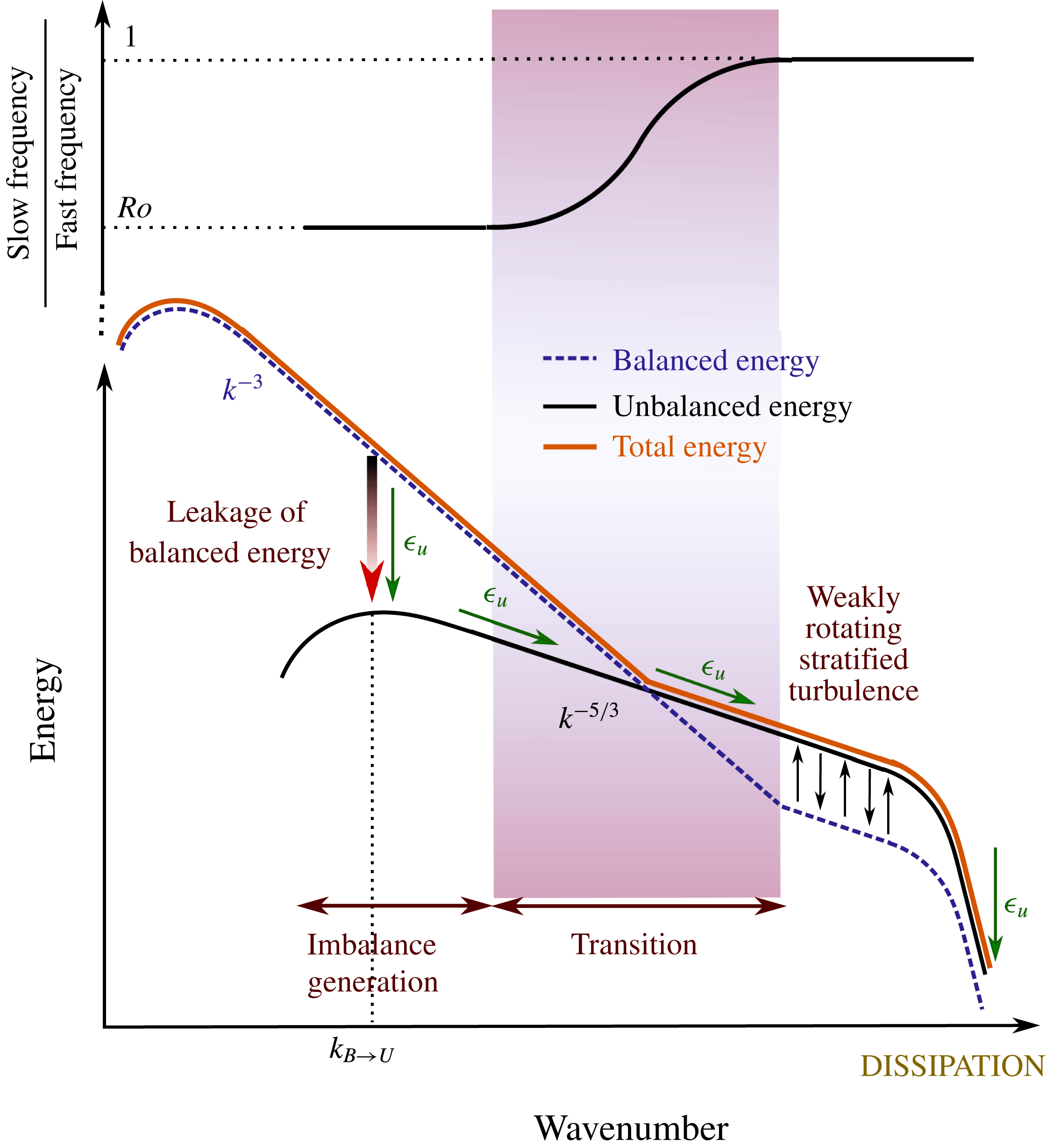
The quantification of imbalance generation can also shed light on the mechanisms that transition the large-scale balanced dynamics to the unbalanced mesoscale dynamics in the atmosphere (or submesoscale dynamics in the ocean). This transition was observed in atmospheric data by Nastrom & Gage (Reference Nastrom and Gage1985) and Lindborg (Reference Lindborg1999). According to these observations, the atmospheric energy spectrum has a slope of
 $-3$
at synoptic scales. This power-law scaling is explained by the theory of geostrophic turbulence (Charney Reference Charney1971). However, at the mesoscales, the energy spectrum develops a shallow tail with a slope of
 $-5/3$
. The steep part of the spectrum at large scales can be viewed as balanced, and much evidence implies that the shallow tail is unbalanced (e.g. see Bartello Reference Bartello2010; Molemaker et al.
Reference Molemaker, McWilliams and Capet2010; Nadiga Reference Nadiga2014; Lindborg Reference Lindborg2015; Kafiabad & Bartello Reference Kafiabad and Bartello2016). Many turbulence studies have been performed to understand the physics behind this transition. Some, such as those of Lindborg (Reference Lindborg2005) and Waite & Bartello (Reference Waite and Bartello2006), focused on strongly stratified turbulence. For instance, Waite & Bartello (Reference Waite and Bartello2006) started from weak rotation with a forward cascade of energy and then decreased
 $Ro$
until an inverse energy cascade appeared. By contrast, more recent rotating stratified turbulence studies have focused on small
 $Ro$
with no significant forward cascade of energy and by weakening the rotation investigated the onset of the forward cascade (Bartello Reference Bartello2010; Vallgren, Deusebio & Lindborg Reference Vallgren, Deusebio and Lindborg2011; Deusebio et al.
Reference Deusebio, Vallgren and Lindborg2013; Marino et al.
Reference Marino, Mininni, Rosenberg and Pouquet2013; Pouquet & Marino Reference Pouquet and Marino2013). The latter approach seems to be more relevant to the development of the shallow mesoscale spectrum. Some of these studies, such as those of Marino et al. (Reference Marino, Mininni, Rosenberg and Pouquet2013), Pouquet & Marino (Reference Pouquet and Marino2013) and Marino et al. (Reference Marino, Rosenberg, Herbert and Pouquet2015), used random forcing in their simulation, whereas others, such as those of Bartello (Reference Bartello2010), Vallgren et al. (Reference Vallgren, Deusebio and Lindborg2011) and Deusebio et al. (Reference Deusebio, Vallgren and Lindborg2013), only forced geostrophic modes. Since geostrophic forcing is linearly balanced, it can more realistically model the large-scale dynamics. Taking balance to higher orders, Kafiabad & Bartello (Reference Kafiabad and Bartello2016) initialised the flow with nonlinearly balanced conditions that included both geostrophic and ageostrophic parts. In this study, after analysing the results based on the definition of linear and nonlinear balance, we find some similarities. Hence, certain qualitative results of previous studies that employed linear balance, such as those of Bartello (Reference Bartello2010), Vallgren et al. (Reference Vallgren, Deusebio and Lindborg2011) and Deusebio et al. (Reference Deusebio, Vallgren and Lindborg2013), can reliably describe the transition from the synoptic to the mesoscale spectrum from a turbulence point of view.
This study, as well as most turbulence studies that have investigated the mesoscale energy spectrum, relies on periodic geometry to have statistical homogeneity. Since atmospheric data were collected close to the tropopause, one may cast doubt on the relevance of triply periodic simulations. In other words, the internal boundary-induced mechanisms may play a more important role in generating imbalance than the fluid interior. A recent study by Asselin, Bartello & Straub (Reference Asselin, Bartello and Straub2018) investigated the comparative significance of these two mechanisms at different Rossby numbers. The authors preformed two sets of simulations: one with constant stratification and the other with a rapid change in the background stratification (which models the tropopause). Starting with QG initial conditions, they found that at characteristic velocities around
 $1~\text{m}~\text{s}^{-1}$
, the former maintains a steep spectrum, while the latter develops a shallow spectrum. This transition from a steep to a shallow slope is consistent with surface quasigeostrophy (SQG), as suggested by Tulloch & Smith (Reference Tulloch and Smith2006). However, for more typical atmospheric Rossby numbers (characteristic velocities of
 $10~\text{m}~\text{s}^{-1}$
), the dynamics with and without a tropopause were reported to be similar. Their results highlight the importance of internal processes in the breakdown of balance and the shallowing of the mesoscale spectrum, which is the focus of this work.
This study can also be viewed as a response to a call for the investigation of balanced turbulence. As mentioned before, most previous studies of balance dynamics relied on either low-order models or special solutions of the governing equations. In his comprehensive review, Vanneste (Reference Vanneste2013) expressed a need to extend balanced methods ‘to treat PDE models and clarify how the full spatiotemporal structure of the balanced motion controls IGW generation’. The current study, which investigates imbalance generation from a rotating stratified turbulence perspective, addresses this need.
This paper is organised as follows. After this introduction, we demonstrate our approach to deriving the transfer between balance and imbalance. This is followed by a section that lays out the specifications of our system as well as the numerical configuration. In the results section, we first compare imbalance generation for different orders of balance. We then analyse the spectrum of transfer to unbalanced motion to find the scales at which most of the balanced energy leaks out. After this, we investigate the effect of different parameters (such as
 $Ro$
and
 $N/f$
) on spontaneous imbalance. We also present a comprehensive section on time scales which investigates the frequency spectra of the different flow regimes. The conclusions are offered in § 5.
2 Theory
2.1 Governing equations and balance dynamics
We consider the non-hydrostatic Boussinesq equation on an
 $f$
-plane, written as
 $$\begin{eqnarray}\displaystyle & \displaystyle \frac{\unicode[STIX]{x2202}\boldsymbol{u}}{\unicode[STIX]{x2202}t}+\boldsymbol{u}\boldsymbol{\cdot }\unicode[STIX]{x1D735}\boldsymbol{u}+f\hat{\boldsymbol{z}}\times \boldsymbol{u}=-\unicode[STIX]{x1D735}p+b\hat{\boldsymbol{z}}+\boldsymbol{D}_{\boldsymbol{u}}, & \displaystyle\end{eqnarray}$$
 $$\begin{eqnarray}\displaystyle & \unicode[STIX]{x1D735}\boldsymbol{\cdot }\boldsymbol{u}=0, & \displaystyle\end{eqnarray}$$
 $$\begin{eqnarray}\displaystyle & \displaystyle \frac{\unicode[STIX]{x2202}b}{\unicode[STIX]{x2202}t}+\boldsymbol{u}\boldsymbol{\cdot }\unicode[STIX]{x1D735}b=-N^{2}w+D_{b}, & \displaystyle\end{eqnarray}$$
 $\boldsymbol{u}$
is the velocity vector,
 $p$
is the pressure perturbation and
 $b$
is the buoyancy perturbation. The operator
 $D_{q}$
represents the dissipation of quantity
 $q$
. Since we are considering large-scale geophysical flows, we neglect the dissipation in our theoretical analysis. Nevertheless, we include it in our numerical simulations to balance the budget of energy. The Brunt–Väisälä frequency
 $N$
and the Coriolis parameter
 $f$
are assumed to be constant.
Instead of velocity components and buoyancy, (2.1) can be expressed in terms of fast and slow modes in the following abstract form (see Warn et al. Reference Warn, Bokhove, Shepherd and Vallis1995; Vanneste Reference Vanneste2013):
 $$\begin{eqnarray}\displaystyle & \displaystyle \frac{\unicode[STIX]{x2202}\boldsymbol{s}}{\unicode[STIX]{x2202}t}=\boldsymbol{N}_{\boldsymbol{s}}(\boldsymbol{s},\boldsymbol{f}), & \displaystyle\end{eqnarray}$$
 $$\begin{eqnarray}\displaystyle & \displaystyle \frac{\unicode[STIX]{x2202}\boldsymbol{f}}{\unicode[STIX]{x2202}t}+\unicode[STIX]{x1D71E}\boldsymbol{f}=\boldsymbol{N}_{\boldsymbol{f}}(\boldsymbol{s},\boldsymbol{f}), & \displaystyle\end{eqnarray}$$
 $\boldsymbol{N}_{\boldsymbol{s}}$
and
 $\boldsymbol{N}_{\boldsymbol{f}}$
are nonlinear functions and
 $\unicode[STIX]{x1D71E}$
is a linear matrix. Here,
 $\boldsymbol{s}$
and
 $\boldsymbol{f}$
denote the slow and fast modes respectively. The flow variables may be decomposed to slow and fast modes in different ways. For instance, Mohebalhojeh & Dritschel (Reference Mohebalhojeh and Dritschel2001) considered the total potential vorticity (PV) as the slow variable and the horizontal divergence and the ageostrophic vorticity as the fast variables. Others such as Baer & Tribbia (Reference Baer and Tribbia1977) and Leith (Reference Leith1980) made their choice of variables based on the normal modes of the linearised equations. Regardless of how these modes are chosen, there are no linear terms in (2.2a
). Hence, the advective time scale (
 $T=L/U$
) characterises the evolution of
 $\boldsymbol{s}$
. On the other hand, the linear term in (2.2b
) may lead to a fast time scale (
 $t^{\ast }$
) for
 $\boldsymbol{f}$
, which is determined by the imaginary part of the eigenvalues of
 $\unicode[STIX]{x1D6E4}$
. It should be noted that
 $\boldsymbol{f}$
may vary on the slow time scale as well. In fact, we will discuss below how the slowly varying component of
 $\boldsymbol{f}$
contributes to high-order balance models. After comparing the two time scales, one finds
 $T=\unicode[STIX]{x1D716}t^{\ast }$
, where
 $\unicode[STIX]{x1D716}$
is a small parameter proportional to
 $Ro$
(e.g. see Vanneste Reference Vanneste2013). Hence, the time derivative can be decomposed into fast and slow components as follows:
 $$\begin{eqnarray}\frac{\unicode[STIX]{x2202}(\,)}{\unicode[STIX]{x2202}t}=\frac{\unicode[STIX]{x2202}(\,)}{\unicode[STIX]{x2202}t^{\ast }}+\unicode[STIX]{x1D716}\frac{\unicode[STIX]{x2202}(\,)}{\unicode[STIX]{x2202}T}.\end{eqnarray}$$
After non-dimensionalising (2.2) and using (2.3), we derive
 $$\begin{eqnarray}\displaystyle & \displaystyle \frac{\unicode[STIX]{x2202}\boldsymbol{s}}{\unicode[STIX]{x2202}t^{\ast }}+\unicode[STIX]{x1D716}\frac{\unicode[STIX]{x2202}\boldsymbol{s}}{\unicode[STIX]{x2202}T}=\unicode[STIX]{x1D716}\boldsymbol{N}_{\boldsymbol{s}}(\boldsymbol{s},\boldsymbol{f}), & \displaystyle\end{eqnarray}$$
 $$\begin{eqnarray}\displaystyle & \displaystyle \frac{\unicode[STIX]{x2202}\boldsymbol{f}}{\unicode[STIX]{x2202}t^{\ast }}+\unicode[STIX]{x1D716}\frac{\unicode[STIX]{x2202}\boldsymbol{f}}{\unicode[STIX]{x2202}T}+\unicode[STIX]{x1D6E4}\boldsymbol{f}=\unicode[STIX]{x1D716}\boldsymbol{N}_{\boldsymbol{f}}(\boldsymbol{s},\boldsymbol{f}). & \displaystyle\end{eqnarray}$$
 $t^{\ast }$
, which leaves the nonlinear interaction of the fast modes with themselves. We restrict ourselves to more traditional balance models, which remove the fast time scale by scale analysis and expansions in terms of the small parameter
 $\unicode[STIX]{x1D716}$
(instead of averaging over
 $t^{\ast }$
). After expanding
 $\boldsymbol{f}$
in terms of
 $\unicode[STIX]{x1D716}$
in (2.4), the leading-order balance dynamics are derived as
 $$\begin{eqnarray}\displaystyle & \displaystyle \frac{\unicode[STIX]{x2202}\boldsymbol{s}}{\unicode[STIX]{x2202}T}=\boldsymbol{N}_{\boldsymbol{s}}(\boldsymbol{s},0), & \displaystyle\end{eqnarray}$$
 $$\begin{eqnarray}\displaystyle & \boldsymbol{f}=0. & \displaystyle\end{eqnarray}$$
 $\boldsymbol{s}=\boldsymbol{s}(T)$
). If
 $\boldsymbol{f}=0$
in (2.4b
), the right-hand side of this equation would be non-zero (
 $\boldsymbol{N}_{\boldsymbol{f}}(\boldsymbol{s},0)\neq 0$
). Hence, it would inevitably generate fast motion in time. To limit this generation, higher-order balance is required. To that end, we seek solutions to (2.4b
) such that
 $\text{d}\boldsymbol{f}/\text{d}t^{\ast }=0$
. The relationship between the remaining terms in (2.4b
) that balance one another can be written in the following generic form:
 $$\begin{eqnarray}\boldsymbol{f}^{b}=\boldsymbol{H}(\boldsymbol{s};\unicode[STIX]{x1D716}).\end{eqnarray}$$
We use the superscript
 $b$
to emphasise that
 $\boldsymbol{f}^{b}$
is a function of only
 $T$
and no longer independently varying. In the context of balance dynamics, (2.6) is known as the slave or balance relation, and
 $\boldsymbol{s}$
and
 $\boldsymbol{f}^{b}$
are referred to as the slaving and slaved variables respectively (Leith Reference Leith1980; Lorenz Reference Lorenz1986; Warn et al.
Reference Warn, Bokhove, Shepherd and Vallis1995).
To derive an expression for (2.6),
 $\boldsymbol{f}^{b}$
can be expanded in terms of
 $\unicode[STIX]{x1D716}$
,
 $$\begin{eqnarray}\boldsymbol{f}^{b}=\unicode[STIX]{x1D6FC}+\unicode[STIX]{x1D716}\unicode[STIX]{x1D6FC}^{\prime }+\unicode[STIX]{x1D716}^{2}\unicode[STIX]{x1D6FC}^{\prime \prime }+O(\unicode[STIX]{x1D716}^{3}).\end{eqnarray}$$
According to (2.5b
),
 $\boldsymbol{f}^{b}$
is zero at
 $O(\unicode[STIX]{x1D716}^{0})$
. Hence,
 $\unicode[STIX]{x1D6FC}=0$
. The next-order balance is derived by keeping the terms at
 $O(\unicode[STIX]{x1D716})$
in (2.4b
) (while setting
 $\text{d}\boldsymbol{f}/\text{d}t^{\ast }=0$
),
 $$\begin{eqnarray}\boldsymbol{f}^{b}=\unicode[STIX]{x1D716}\unicode[STIX]{x1D6FC}^{\prime }=\unicode[STIX]{x1D716}\unicode[STIX]{x1D6E4}^{-1}\boldsymbol{N}_{\boldsymbol{ f}}(\boldsymbol{s},0),\end{eqnarray}$$
which is the first-order approximation for (2.6). Many balance models share (2.8) as their leading-order correction to linear balance (e.g. Baer & Tribbia Reference Baer and Tribbia1977; Machenhauer Reference Machenhauer1977; Warn et al.
Reference Warn, Bokhove, Shepherd and Vallis1995). As shown by Baer & Tribbia (Reference Baer and Tribbia1977) and Warn et al. (Reference Warn, Bokhove, Shepherd and Vallis1995), higher orders of balance are derived systematically by expanding the terms up to higher orders in (2.4b
). In this study, we calculate balance up to
 $O(\unicode[STIX]{x1D716}^{2})$
and compare the results of zeroth-, first- and second-order balance. The derivation of second-order balance is presented in appendix A.
2.2 The interaction between balance and imbalance in the context of the full equations
Equations (2.5a
) and (2.6) together form a balance model that approximates (2.2). However, even at relatively low
 $Ro$
and
 $Fr$
, the solutions of balance models and the full equations may differ in time at least at certain scales (Molemaker et al.
Reference Molemaker, McWilliams and Capet2010; Nadiga Reference Nadiga2014; Kafiabad & Bartello Reference Kafiabad and Bartello2016). Therefore, it is enlightening to study balance dynamics in the context of the full equations to investigate to what extent, when and where it breaks down. The first step in such a study is to decompose solutions of (2.1) into a balanced part,
 $\{\boldsymbol{s},\boldsymbol{f}^{b}\}$
, and an unbalanced part,
 $\boldsymbol{f}^{u}=\boldsymbol{f}-\boldsymbol{f}^{b}$
. This can be readily done by using the definition of
 $\boldsymbol{s}$
and
 $\boldsymbol{f}^{b}$
in a balance model. Many studies performed this decomposition based on the definition of linear balance in (2.5) (among others, Bartello Reference Bartello2010; Deusebio et al.
Reference Deusebio, Vallgren and Lindborg2013; Nadiga Reference Nadiga2014). More recently, Kafiabad & Bartello (Reference Kafiabad and Bartello2017) employed a higher-order nonlinear balance for such an analysis.
In addition to decomposing a flow into a balanced and an unbalanced component, it is insightful to find how they interact with each other in the context of the full dynamics. A balance model on its own cannot describe these interactions. To see this more clearly, we can write the slow-time evolution of balance variables together as
 $$\begin{eqnarray}\displaystyle & \displaystyle \frac{\unicode[STIX]{x2202}\boldsymbol{s}}{\unicode[STIX]{x2202}T}=\boldsymbol{N}_{\boldsymbol{s}}(\boldsymbol{s},0), & \displaystyle\end{eqnarray}$$
 $$\begin{eqnarray}\displaystyle & \displaystyle \frac{\unicode[STIX]{x2202}\boldsymbol{f}^{b}}{\unicode[STIX]{x2202}T}=\frac{\unicode[STIX]{x2202}\boldsymbol{H}}{\unicode[STIX]{x2202}\boldsymbol{s}}\frac{\unicode[STIX]{x2202}\boldsymbol{s}}{\unicode[STIX]{x2202}T}=\frac{\unicode[STIX]{x2202}\boldsymbol{H}}{\unicode[STIX]{x2202}\boldsymbol{s}}\boldsymbol{N}_{\boldsymbol{s}}(\boldsymbol{s},0), & \displaystyle\end{eqnarray}$$
 $$\begin{eqnarray}\displaystyle & \displaystyle \frac{\unicode[STIX]{x2202}\boldsymbol{s}}{\unicode[STIX]{x2202}t}=\unicode[STIX]{x1D716}\boldsymbol{N}_{\boldsymbol{s}}(\boldsymbol{s},\boldsymbol{f}^{b}+\boldsymbol{f}^{u}), & \displaystyle\end{eqnarray}$$
 $$\begin{eqnarray}\displaystyle & \displaystyle \frac{\unicode[STIX]{x2202}(\boldsymbol{f}^{b}+\boldsymbol{f}^{u})}{\unicode[STIX]{x2202}t}+\unicode[STIX]{x1D6E4}(\boldsymbol{f}^{b}+\boldsymbol{f}^{u})=\unicode[STIX]{x1D716}\boldsymbol{N}_{\boldsymbol{ f}}(\boldsymbol{s},\boldsymbol{f}^{b}+\boldsymbol{f}^{u}). & \displaystyle\end{eqnarray}$$
 $\boldsymbol{N}_{\boldsymbol{f}}(\boldsymbol{s},\boldsymbol{f}^{b}+\boldsymbol{f}^{u})$
is transferred to
 $\boldsymbol{f}^{b}$
and what portion to
 $\boldsymbol{f}^{u}$
. If
 $\boldsymbol{f}^{b}$
and
 $\boldsymbol{f}^{u}$
are orthogonal, we can separate the transfer of energy by taking the scalar product of (2.10b
) with
 $\boldsymbol{f}^{b}$
and
 $\boldsymbol{f}^{u}$
separately (it should be noted that in this case the scalar product of
 $\boldsymbol{f}^{b}$
and
 $\boldsymbol{f}^{u}$
is zero). However,
 $\boldsymbol{f}^{b}$
and
 $\boldsymbol{f}^{u}$
are not necessarily orthogonal for nonlinear balance models. Below, we suggest a systematic approach to derive separate equations for the time evolutions of
 $\boldsymbol{f}^{b}$
and
 $\boldsymbol{f}^{u}$
, which can be applied to any balance–imbalance decomposition as long as the flow is predominantly balanced. In this case, the slave relation (2.6) is still a good approximation that relates
 $\boldsymbol{s}$
to
 $\boldsymbol{f}^{b}$
. The time derivative of this relation in the context of the full dynamics is
 $$\begin{eqnarray}\frac{\unicode[STIX]{x2202}\boldsymbol{f}^{b}}{\unicode[STIX]{x2202}t}=\frac{\unicode[STIX]{x2202}\boldsymbol{H}}{\unicode[STIX]{x2202}\boldsymbol{s}}\frac{\unicode[STIX]{x2202}\boldsymbol{s}}{\unicode[STIX]{x2202}t}.\end{eqnarray}$$
We emphasise that
 $\unicode[STIX]{x2202}\boldsymbol{f}^{b}/\unicode[STIX]{x2202}t$
and
 $\unicode[STIX]{x2202}\boldsymbol{s}/\unicode[STIX]{x2202}t$
described by (2.11) and (2.10a
) are the time evolutions of the balanced modes according to the full equations, whereas
 $\unicode[STIX]{x2202}\boldsymbol{f}^{b}/\unicode[STIX]{x2202}T$
and
 $\unicode[STIX]{x2202}\boldsymbol{s}/\unicode[STIX]{x2202}T$
are the slow-time evolutions of these modes according to the reduced balance model. Therefore,
 $\unicode[STIX]{x2202}\boldsymbol{s}/\unicode[STIX]{x2202}t$
in (2.11) should be replaced by (2.10a
), where the balanced modes interact with
 $\boldsymbol{f}^{u}$
and may have a fast time scale
 $$\begin{eqnarray}\frac{\unicode[STIX]{x2202}\boldsymbol{f}^{b}}{\unicode[STIX]{x2202}t}=\frac{\unicode[STIX]{x2202}\boldsymbol{H}}{\unicode[STIX]{x2202}\boldsymbol{s}}\unicode[STIX]{x1D716}\boldsymbol{N}_{\boldsymbol{s}}(\boldsymbol{s},\boldsymbol{f}^{b}+\boldsymbol{f}^{u}).\end{eqnarray}$$
This expression can be calculated for first-order balance, by taking
 $\unicode[STIX]{x2202}/\unicode[STIX]{x2202}t$
of (2.8),
 $$\begin{eqnarray}\frac{\unicode[STIX]{x2202}\boldsymbol{f}^{b}}{\unicode[STIX]{x2202}t}=\unicode[STIX]{x1D716}\frac{\unicode[STIX]{x2202}\unicode[STIX]{x1D6FC}^{\prime }}{\unicode[STIX]{x2202}t}=\frac{\unicode[STIX]{x2202}}{\unicode[STIX]{x2202}t}\unicode[STIX]{x1D716}\unicode[STIX]{x1D6E4}^{-1}\boldsymbol{N}_{\boldsymbol{ f}}(\boldsymbol{s},0)=\unicode[STIX]{x1D716}\unicode[STIX]{x1D6E4}^{-1}\left[\boldsymbol{N}_{\boldsymbol{ f}}\left(\boldsymbol{s}+\frac{\unicode[STIX]{x2202}\boldsymbol{s}}{\unicode[STIX]{x2202}t},0\right)-\boldsymbol{N}_{\boldsymbol{f}}(\boldsymbol{s},0)-\boldsymbol{N}_{\boldsymbol{f}}\left(\frac{\unicode[STIX]{x2202}\boldsymbol{s}}{\unicode[STIX]{x2202}t},0\right)\right].\end{eqnarray}$$
We employed the fact that
 $\boldsymbol{N}_{\boldsymbol{f}}(\boldsymbol{s},0)$
is quadratic with respect to
 $\boldsymbol{s}$
to derive the last expression in (2.13). Substitution of
 $\unicode[STIX]{x2202}\boldsymbol{s}/\unicode[STIX]{x2202}t$
with (2.10a
) in this equation leads to
 $$\begin{eqnarray}\displaystyle \frac{\unicode[STIX]{x2202}\boldsymbol{f}^{b}}{\unicode[STIX]{x2202}t} & = & \displaystyle \unicode[STIX]{x1D716}\frac{\unicode[STIX]{x2202}\unicode[STIX]{x1D6FC}^{\prime }}{\unicode[STIX]{x2202}t}=\unicode[STIX]{x1D716}\unicode[STIX]{x1D6E4}^{-1}[\boldsymbol{N}_{\boldsymbol{ f}}(\boldsymbol{s}+\boldsymbol{N}_{\boldsymbol{s}}(\boldsymbol{s},\boldsymbol{f}^{b}+\boldsymbol{f}^{u}),0)-\boldsymbol{N}_{\boldsymbol{ f}}(\boldsymbol{s},0)-\boldsymbol{N}_{\boldsymbol{f}}(\boldsymbol{N}_{\boldsymbol{s}}(\boldsymbol{s},\boldsymbol{f}^{b}+\boldsymbol{f}^{u}),0)]\nonumber\\ \displaystyle & = & \displaystyle \unicode[STIX]{x1D716}\boldsymbol{M}(\boldsymbol{s},\boldsymbol{f}^{b},\boldsymbol{f}^{u}).\end{eqnarray}$$
Subtraction of (2.14) from (2.10b ) gives the evolution of the unbalanced modes,
 $$\begin{eqnarray}\frac{\unicode[STIX]{x2202}\boldsymbol{f}^{u}}{\unicode[STIX]{x2202}t}+\unicode[STIX]{x1D6E4}(\boldsymbol{f}^{b}+\boldsymbol{f}^{u})=\unicode[STIX]{x1D716}[\boldsymbol{N}_{\boldsymbol{ f}}(\boldsymbol{s},\boldsymbol{f}^{b}+\boldsymbol{f}^{u})-\boldsymbol{M}(\boldsymbol{s},\boldsymbol{f}^{b},\boldsymbol{f}^{u})]=\boldsymbol{Q}(\boldsymbol{s},\boldsymbol{f}^{b},\boldsymbol{f}^{u}).\end{eqnarray}$$
Similarly to the definition of balance,
 $\unicode[STIX]{x2202}\boldsymbol{f}^{b}/\unicode[STIX]{x2202}t$
can be derived systematically at different orders by expanding (2.2b
) in terms of
 $\unicode[STIX]{x1D716}$
and using (2.10a
) (instead of (2.9a
)) to replace
 $\unicode[STIX]{x2202}\boldsymbol{s}/\unicode[STIX]{x2202}t$
. We perform this procedure up to second order in appendix B and compare it with those of lower orders in the results section.
2.3 Normal-mode decomposition
As mentioned earlier, the flow variables can be decomposed into
 $\boldsymbol{s}$
and
 $\boldsymbol{f}$
in different ways. The method introduced in the previous section can be applied to any choice of
 $\boldsymbol{s}$
and
 $\boldsymbol{f}$
as long as the governing equations take the form of (2.2). In this study, we employ the normal modes of the linearised equations, following Baer & Tribbia (Reference Baer and Tribbia1977), Leith (Reference Leith1980) and Bartello (Reference Bartello1995). This requires the boundaries to be periodic, which also allows statistical homogeneity. After transforming (2.1) to Fourier space, we can write it as
 $$\begin{eqnarray}\frac{\text{d}\boldsymbol{X}_{\boldsymbol{k}}}{\text{d}t}=-\text{i}\unicode[STIX]{x1D647}_{\boldsymbol{k}}\boldsymbol{X}_{\boldsymbol{k}}+\boldsymbol{N}_{\boldsymbol{k}}(\boldsymbol{X}),\end{eqnarray}$$
where all of the flow variables (such as velocity components and buoyancy) are grouped together and presented in the state vector
 $\boldsymbol{X}_{\boldsymbol{k}}$
. The matrix
 $\unicode[STIX]{x1D647}_{\boldsymbol{k}}$
represents the linear terms and the function
 $\boldsymbol{N}_{\boldsymbol{k}}$
represents the nonlinear terms. With the assumption of periodicity, the wavevector
 $\boldsymbol{k}=(k_{x},k_{y},k_{z})$
becomes discrete. Hence, it is considered as an index for the flow variables. If the variables in
 $\boldsymbol{X}$
are appropriately chosen,
 $\unicode[STIX]{x1D647}_{\boldsymbol{k}}$
becomes Hermitian, with corresponding orthogonal eigenvectors and real eigenvalues as follows:
 $$\begin{eqnarray}\unicode[STIX]{x1D706}_{\boldsymbol{k}}^{(0)}=0,\quad \unicode[STIX]{x1D706}_{\boldsymbol{ k}}^{\pm }=\pm \unicode[STIX]{x1D70E}_{\boldsymbol{ k}}=\pm \frac{(f^{2}{k_{z}}^{2}+N^{2}{k_{h}}^{2})^{1/2}}{k},\end{eqnarray}$$
where
 $k_{h}=(k_{x}^{2}+k_{y}^{2})^{1/2}$
and
 $k=(k_{h}^{2}+k_{z}^{2})^{1/2}$
. The normal modes are then derived by projecting
 $\boldsymbol{X}_{\boldsymbol{k}}$
onto the eigenvectors. Following Bartello (Reference Bartello1995), we call the modes associated with
 $\unicode[STIX]{x1D706}_{\boldsymbol{k}}^{(0)}$
geostrophic and those associated with
 $\unicode[STIX]{x1D706}_{\boldsymbol{k}}^{(\pm )}$
ageostrophic, and denote them by
 $G_{\boldsymbol{k}}$
and
 $A_{\boldsymbol{k}}$
respectively. We then define
 $\boldsymbol{s}=G_{\boldsymbol{k}}$
and
 $\boldsymbol{f}=A_{\boldsymbol{k}}$
. Consequently, we denote the balanced and unbalanced parts of
 $\boldsymbol{f}$
with
 $A_{\boldsymbol{k}}^{b}$
and
 $A_{\boldsymbol{k}}^{u}$
. More detail on the normal-mode decomposition can be found in Leith (Reference Leith1980) and Bartello (Reference Bartello1995).
2.4 Energy and transfer spectra
We define the geostrophic and ageostrophic energy spectra as follows:
 $$\begin{eqnarray}E_{G}(k_{h})=\sum \unicode[STIX]{x1D6FC}_{\boldsymbol{k}}\langle G_{\boldsymbol{k}},G_{\boldsymbol{k}}\rangle ,\quad E_{A}(k_{h})=\sum \unicode[STIX]{x1D6FC}_{\boldsymbol{k}}\langle A_{\boldsymbol{k}},A_{\boldsymbol{k}}\rangle ,\end{eqnarray}$$
where the scalar product is defined as
 $\langle A,A\rangle \equiv A_{i}{A_{i}}^{\ast }$
(
 $i$
being a dummy index and
 $A^{\ast }$
the complex conjugate of
 $A$
). The summations are carried over cylindrical shells (with varying
 $k_{z}$
and constant
 $k_{h}$
) to derive horizontal energy spectra, which enables us to compare our results with the observed atmospheric data (e.g. Nastrom & Gage Reference Nastrom and Gage1985). Depending on how
 $G_{\boldsymbol{k}}$
and
 $A_{\boldsymbol{k}}$
are defined, the terms inside the summations may not have the same dimension as the energy spectrum. Hence, the constant
 $\unicode[STIX]{x1D6FC}_{\boldsymbol{k}}$
(which may be a function of
 $k_{h}$
) is introduced to keep the dimensions consistent. An appropriate choice of
 $\unicode[STIX]{x1D6FC}$
also leads to
 $E=E_{G}+E_{A}$
, where
 $E$
is the total energy spectrum. Following the definition of
 $G_{\boldsymbol{k}}$
and
 $A_{\boldsymbol{k}}$
in Bartello (Reference Bartello1995), we derive
 $\unicode[STIX]{x1D6FC}_{\boldsymbol{k}}=1/(2{k_{h}}^{2})$
. The ageostrophic energy spectrum may be further decomposed into a balanced part
 $E_{A^{b}}$
and an unbalanced part
 $E_{A^{u}}$
,
 $$\begin{eqnarray}E_{A^{b}}(k_{h})=\sum \unicode[STIX]{x1D6FC}_{\boldsymbol{k}}\langle A_{\boldsymbol{k}}^{b},A_{\boldsymbol{ k}}^{b}\rangle ,\quad E_{A^{u}}(k_{h})=\sum \unicode[STIX]{x1D6FC}_{\boldsymbol{k}}\langle A_{\boldsymbol{k}}^{u},A_{\boldsymbol{ k}}^{u}\rangle .\end{eqnarray}$$
The balanced energy can then be defined as
 $E_{B}=E_{G}+E_{A^{b}}$
and the unbalanced energy as
 $E_{U}=E_{A^{u}}$
. We ultimately want to obtain the budget of
 $E_{B}$
and
 $E_{U}$
from the governing equations as
 $$\begin{eqnarray}\displaystyle & \displaystyle \frac{\text{d}}{\text{d}t}E_{\boldsymbol{B}}(k_{h})=T_{B}(k_{h}), & \displaystyle\end{eqnarray}$$
 $$\begin{eqnarray}\displaystyle & \displaystyle \frac{\text{d}}{\text{d}t}E_{\boldsymbol{U}}(k_{h})=T_{U}(k_{h}), & \displaystyle\end{eqnarray}$$
 $T_{B}(k_{h})$
and
 $T_{U}(k_{h})$
are the spectra of energy transferred to the balanced and unbalanced modes respectively. Equation (2.20b
) can be derived by taking the scalar product of (2.15) with
 $\boldsymbol{f}^{u}$
and then summing over cylindrical shells in Fourier space. For the first-order balance–imbalance decomposition, this procedure leads to
 $$\begin{eqnarray}T_{U}(k_{h})=\sum \langle \boldsymbol{Q}_{\boldsymbol{k}},A_{\boldsymbol{k}}^{u}\rangle +\text{c.c.},\end{eqnarray}$$
where c.c. denotes the complex conjugate. A similar expression can be derived for
 $T_{B}$
. The energies
 $E_{B}$
and
 $E_{U}$
may be different for different orders of balance. We compare the results at zeroth, first and second order in this study. For linear balance (i.e. zeroth order),
 $E_{B}=E_{G}$
and
 $E_{U}=E_{A}$
.
3 Numerical settings
The PDEs in (2.1) need a set of ICs to be integrated. As expressed in previous sections, we want the flow to be predominantly balanced. Therefore, we seek sets of
 $\{G_{\boldsymbol{k}}\}$
and
 $\{A_{\boldsymbol{k}}^{b}\}$
as ICs. We obtain
 $\{G_{\boldsymbol{k}}\}$
by running a QG model that has the same resolution and dissipation as the corresponding Boussinesq simulation. Then, we use (2.6) accurate to second order in
 $\unicode[STIX]{x1D716}$
to derive
 $\{A_{\boldsymbol{k}}^{b}\}$
. More detail on producing this initial condition can be found in Kafiabad & Bartello (Reference Kafiabad and Bartello2016).
We employ the de-aliased pseudospectral method with centred time stepping. The size of our domain is set to
 $2\unicode[STIX]{x03C0}$
in the horizontal and to
 $2\unicode[STIX]{x03C0}\times (f/N)$
in the vertical. In this configuration, the aspect ratio,
 $H/L$
, is equal to
 $f/N$
, which makes the domain a cube of
 $(2\unicode[STIX]{x03C0})^{3}$
in the classical QG coordinates (Charney Reference Charney1971). We employ equally spaced grids in physical space, i.e.
 $\unicode[STIX]{x0394}x=\unicode[STIX]{x0394}y=\unicode[STIX]{x0394}z$
. An alternative grid is equally spaced in the scaled coordinate, i.e.
 $\unicode[STIX]{x0394}x=\unicode[STIX]{x0394}y=N/f\unicode[STIX]{x0394}z$
. We compared the results on both grids in Kafiabad & Bartello (Reference Kafiabad and Bartello2017) and expressed the benefits and shortcomings of each. We concluded that the former grid might better suit our study which is focused on the breakdown of balance. Therefore, all simulations in this paper are performed on the isotropic grid.
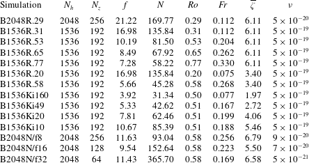
The simulations presented in the following sections are listed in table 1. They employ either 2048 or 1536 grid points in the horizontal. The ratio of horizontal to vertical resolution is
 $N/f$
to keep
 $\unicode[STIX]{x0394}x=\unicode[STIX]{x0394}z$
. For most of our simulations,
 $N/f=8$
. However, we performed several simulations with
 $N/f=16$
and 32 to investigate the effect of
 $N/f$
on the breakdown of balance.
The non-hydrostatic Boussinesq simulations presented in this paper. The values of
 $Ro$
,
 $Fr$
and
 $\overline{\unicode[STIX]{x1D701}}$
are calculated at
 $t=0$
.

All of the simulations in this paper are of decaying turbulence. Nevertheless, forcing with high-order nonlinear balance would yield virtually identical results. This is simply because the length of our simulations is based on the relatively quick spontaneous imbalance and generation of a shallow tail in the spectrum. This is at most a few eddy turnover times during which the energy dissipation is weak. Starting with a jet, as opposed to fully developed QG turbulence, is another matter. First, it is necessary to add the higher-order ageostrophic corrections to the geostrophic jet in order to get something analogous to the high-order balanced IC employed here. Second, after at most a couple more eddy turnover times, the jet would go unstable and we would have an array of eddies much like the fields we used as ICs, which in our view resemble smaller-scale synoptic features in a typical atmosphere, or mesoscale eddies in the ocean.
We use the following form of hyperdissipation for
 $D_{\boldsymbol{u}}$
and
 $D_{b}$
in (2.1):
 $$\begin{eqnarray}D_{\boldsymbol{u},b}=-\unicode[STIX]{x1D708}_{h}\unicode[STIX]{x1D6FB}_{h}^{8}(\boldsymbol{u},b)-\unicode[STIX]{x1D708}_{z}\frac{\unicode[STIX]{x2202}^{8}}{\unicode[STIX]{x2202}z^{8}}(\boldsymbol{u},b).\end{eqnarray}$$
We assume the same dissipation for buoyancy and velocity. Since the flow is expected to be close to isotropic at small scales, we set
 $\unicode[STIX]{x1D708}_{h}=\unicode[STIX]{x1D708}_{z}=\unicode[STIX]{x1D708}$
. All of the times reported in this paper are normalised with
 $\overline{\unicode[STIX]{x1D701}}$
, which is the root-mean-square geostrophic contribution to the vertical vorticity at
 $t=0$
. Hence, the reported values can be considered as initial eddy turnover times.
The non-dimensional parameters in table 1 are calculated as
 $$\begin{eqnarray}Ro=\frac{\overline{\unicode[STIX]{x1D714}_{z}^{2}}^{1/2}}{f},\quad Fr=\frac{\overline{\unicode[STIX]{x1D714}_{x}^{2}+\unicode[STIX]{x1D714}_{y}^{2}}^{1/2}}{N},\end{eqnarray}$$
in which
 $\unicode[STIX]{x1D74E}=(\unicode[STIX]{x1D714}_{x},\unicode[STIX]{x1D714}_{y},\unicode[STIX]{x1D714}_{z})$
is the vorticity vector and an overbar denotes a spatial average.
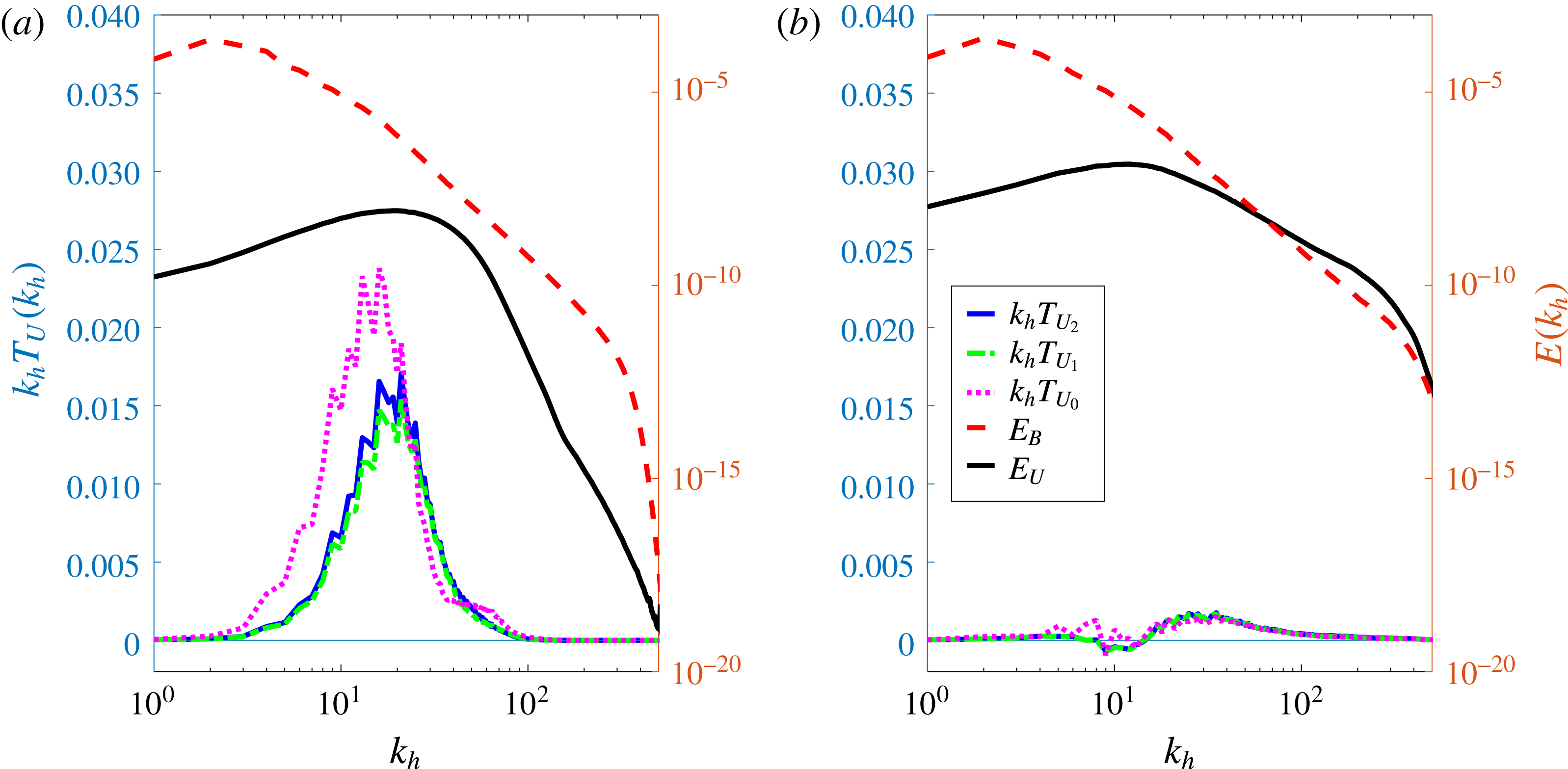
The transfer
 $T_{U}(k_{h})$
, at early times in (a) and at late times in (b). For the early times, the spectra are averaged over the time interval of
 $[0,0.1\overline{\unicode[STIX]{x1D701}}]$
, and for the late times, over
 $[0.4\overline{\unicode[STIX]{x1D701}},0.5\overline{\unicode[STIX]{x1D701}}]$
. The energies
 $E_{B}$
and
 $E_{U}$
of the same simulations are also plotted. The left axis is associated with the transfer spectra and the right axis with the energy spectra. Here,
 $Ro=0.29$
(simulation B2048R.29).

4 Results
4.1 Transfer of energy to unbalanced modes
Figure 1 portrays
 $T_{U}(k_{h})$
at
 $Ro=0.29$
at zeroth, first and second orders (denoted by
 $T_{U_{0}}$
,
 $T_{U_{1}}$
and
 $T_{U_{2}}$
). Here,
 $T_{U_{0}}$
is simply transfer to ageostrophic modes, while
 $T_{U_{1}}$
is derived from (2.21). The transfer
 $T_{U_{2}}$
is calculated by repeating the same procedure laid out in § 2.4 for the second-order balance (which is explained in appendix (B 2)). The balanced and unbalanced energy spectra are also portrayed in the background. The spectra of (a) and (b) are calculated at the beginning and end of the integration period respectively. For this flow,
 $E_{U}$
surpasses
 $E_{B}$
at later times. Hence, the total energy spectrum displays a kink at
 $k_{h}\simeq 60$
. At early times, the energy is transferred to imbalance at scales larger than this kink, where the flow is still predominantly balanced. This transfer generates an unbalanced energy spectrum that peaks at the same wavenumber as
 $T_{U}$
does. This spectrum has a steep slope initially, but it shallows in time, and its peak moves to larger scales. The transfer
 $T_{U}$
decreases considerably in time and its peak moves towards smaller scales. On comparing (a) and (b) of figure 1, we find that the unbalanced transfer mainly happens at the early times, but nevertheless occurs on the slow nonlinear time scale. The solution of a hypothetical balance model would, therefore, break down compared with the Boussinesq equations at early times. This result is robust to our definition of balance, which is after all only approximate. Given that these simulations are decaying, the early period is the one with the highest energy and the largest Rossby numbers. At the later time, there is a negative transfer at very large scales, followed by a positive transfer. This indicates that the unbalanced modes cascade the energy (which they initially received from the balanced modes) forward towards the dissipation range. The lin–log plot of
 $k_{h}~T_{U}$
is area-preserving, which indicates that the net transfer to imbalance is negligible at the end of the simulation.
On comparing different orders, one finds that the zeroth order is somewhat different from the higher orders. The transfer
 $T_{U_{0}}$
is larger than
 $T_{U_{1}}$
and
 $T_{U_{2}}$
, and peaks at smaller wavenumber at the early time. Later, the difference between
 $T_{U_{0}}$
and higher orders decreases, because
 $Ro$
decreases in our decaying simulations and the expansion in (2.7) converges. Comparison of
 $T_{U_{1}}$
and
 $T_{U_{2}}$
at early times shows that they are very similar. They marginally differ at the peak of the transfer spectrum. However, the difference between them is not noticeable at later times as the two curves lie on top of one another at considerably lower amplitude. This comparison demonstrates that first-order balance (in which nonlinear interactions are considered to the leading order) is a good approximation for the relatively low Rossby number of 0.29.
4.2 The contribution of different triads
Since the nonlinearities in the Boussinesq equations are quadratic, the transfer terms in (2.20) are due to interactions between three modes, known as triads (see, e.g., Kraichnan Reference Kraichnan1967). Here, we classify them based on the type of their interactions. For instance,
 $\boldsymbol{B}\boldsymbol{B}\boldsymbol{U}$
represents the interactions between one unbalanced and two balanced modes. Separation of the contributions to
 $T_{B}$
and
 $T_{U}$
according to the type of interaction leads to
 $$\begin{eqnarray}\displaystyle & \displaystyle T_{B}(k_{h})=T_{BB\rightarrow B}(k_{h})+T_{BU\rightarrow B}(k_{h})+T_{UU\rightarrow B}(k_{h}), & \displaystyle\end{eqnarray}$$
 $$\begin{eqnarray}\displaystyle & \displaystyle T_{U}(k_{h})=T_{BB\rightarrow U}(k_{h})+T_{BU\rightarrow U}(k_{h})+T_{UU\rightarrow U}(k_{h}), & \displaystyle\end{eqnarray}$$
 $T_{BU\rightarrow B}(k_{h})$
is the net transfer of all
 $\boldsymbol{B}\boldsymbol{B}\boldsymbol{U}$
interactions to
 $\boldsymbol{B}$
at wavenumber
 $k_{h}$
.
We can numerically calculate the different nonlinear terms defined in (4.1). The term
 $T_{BB\rightarrow U,B}$
is determined by filtering out the unbalanced modes. Similarly,
 $T_{UU\rightarrow U,B}$
is calculated by setting the balanced modes to zero. The term
 $T_{BU\rightarrow U,B}$
is the residual derived by subtracting
 $T_{BB\rightarrow U,B}$
and
 $T_{UU\rightarrow U,B}$
from the total transfer
 $T_{B,U}$
. To simplify the computations, we only consider first-order balance for this decomposition.
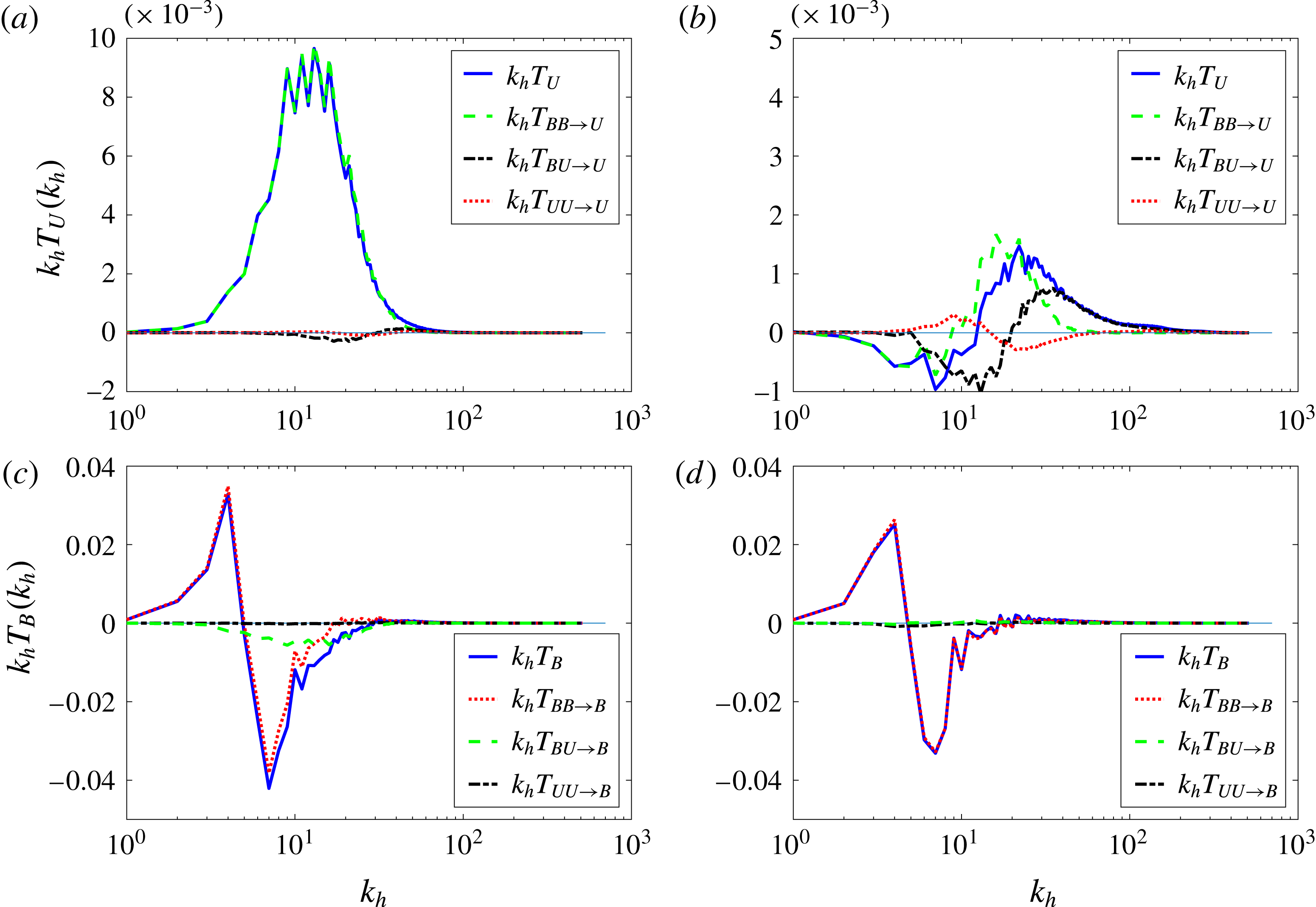
(a,b) Unbalanced transfer spectra. (c,d) Balanced transfer spectra. Here,
 $Ro=0.53$
(simulation B1536R.533). (a,c) The early time (averaged over
 $t~\unicode[STIX]{x1D716}~[0,0.1\overline{\unicode[STIX]{x1D701}}]$
). (b,d) The later time (averaged over
 $t~\unicode[STIX]{x1D716}~[0.4\overline{\unicode[STIX]{x1D701}},0.5\overline{\unicode[STIX]{x1D701}}]$
). The total transfer to balance/imbalance is shown by solid (blue) lines and is decomposed into its constituent triads according to the legends.

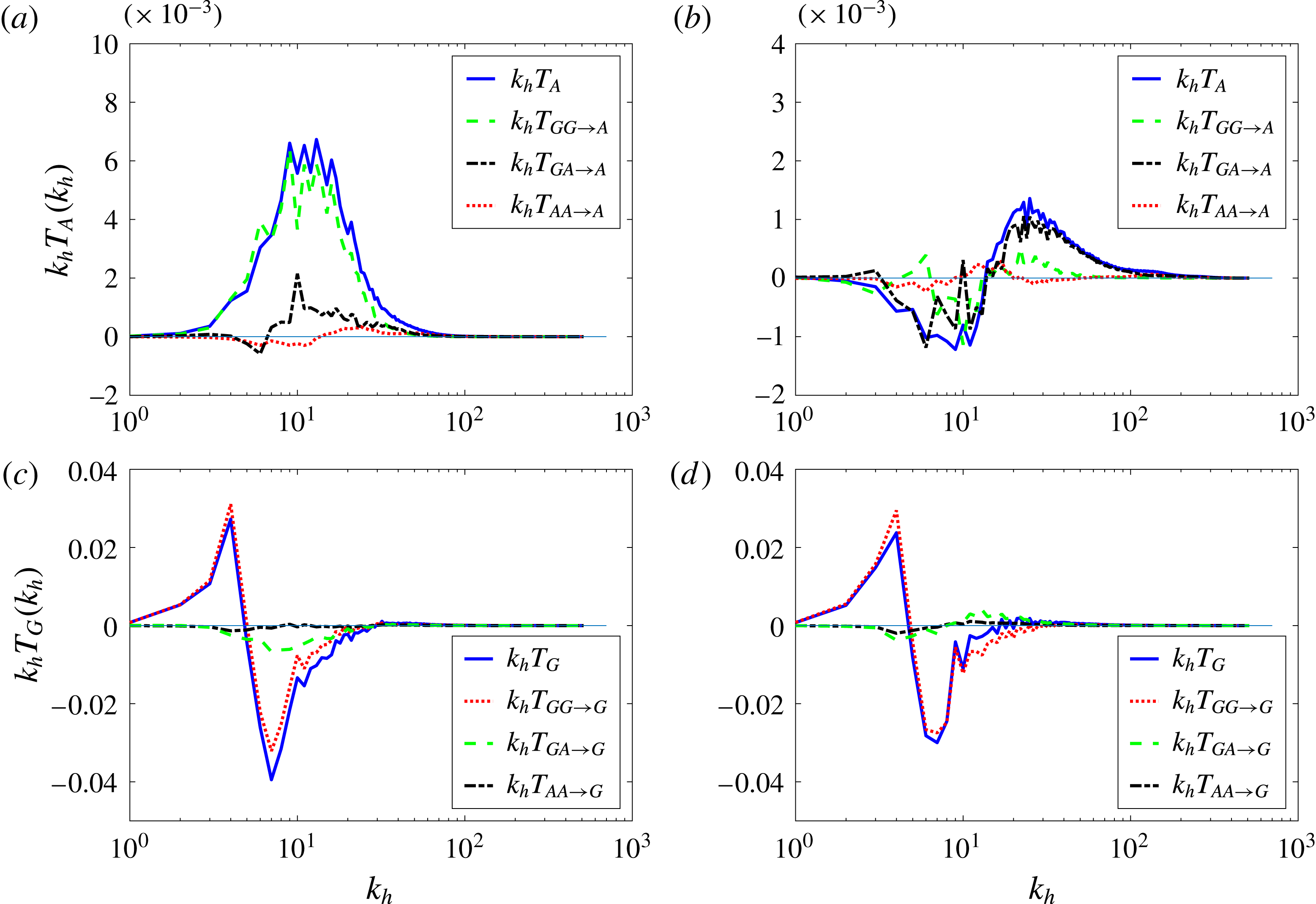
The results of these calculations are shown in figure 2. Panels (a) and (b) display the transfer to unbalanced modes, and panels (c) and (d) the transfer to balanced modes. Panels (a) and (c) correspond to transfer at early times when balance breaks down, and panels (b) and (d) correspond to later times when the shallow tail is developed in the energy spectrum. At early times, the leading-order interaction between balance and imbalance takes place via
 $\boldsymbol{B}\boldsymbol{B}\boldsymbol{U}$
triads since the unbalanced modes tend to zero as
 $t\rightarrow 0$
. This is consistent with figure 2(a), where
 $T_{U}\simeq T_{BB\rightarrow U}$
.
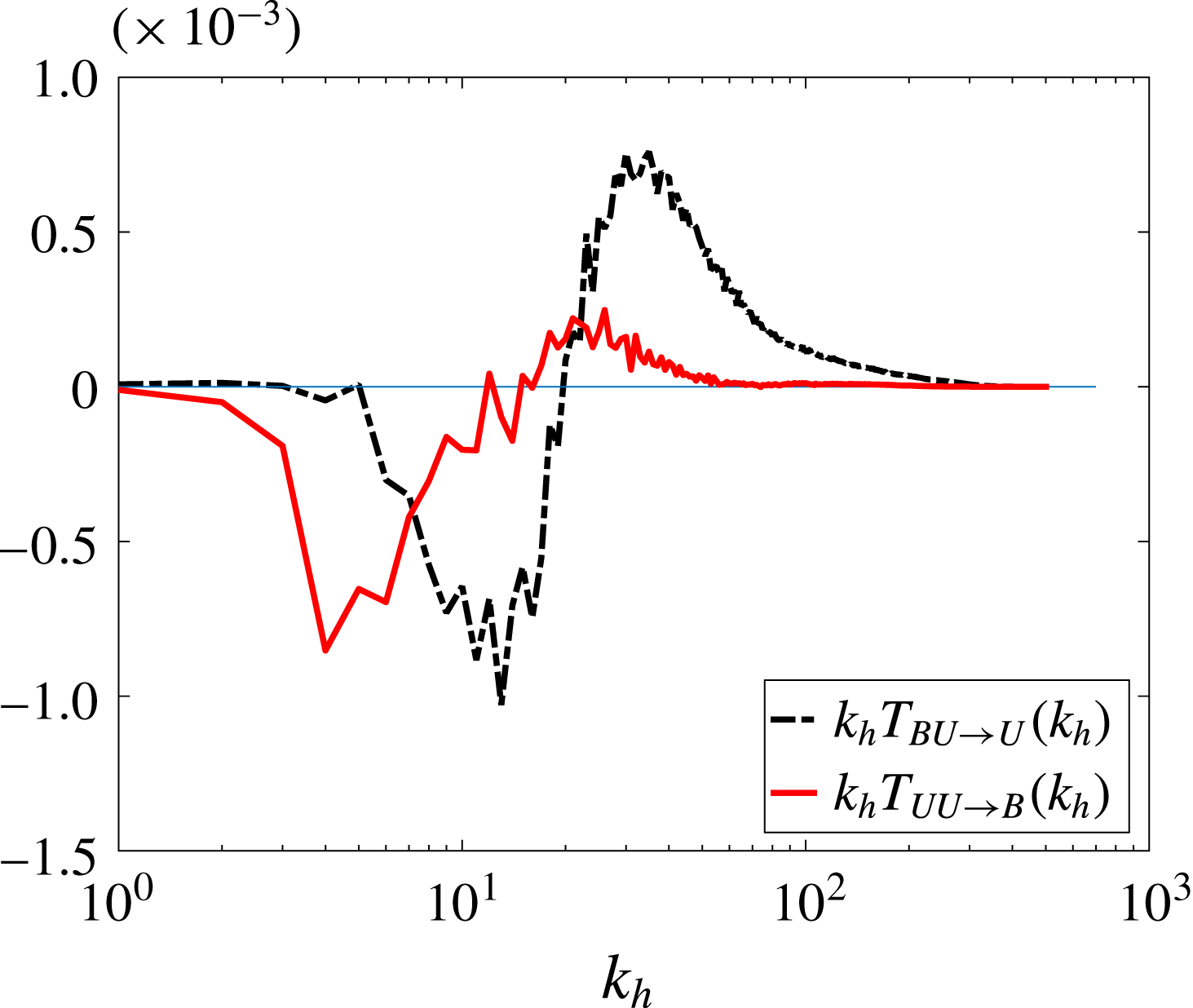
The terms
 $T_{BU\rightarrow U}$
and
 $T_{UU\rightarrow B}$
averaged over
 $[0.4\overline{\unicode[STIX]{x1D701}},0.5\overline{\unicode[STIX]{x1D701}}]$
.

Figure 2(b) shows the transfers to imbalance at the end of the integration time, in which
 $T_{BB\rightarrow U}$
decreases and
 $T_{BU\rightarrow U}$
increases significantly. Therefore, the two terms become comparable but peak at different wavenumbers. Based on this plot,
 $\boldsymbol{B}\boldsymbol{B}\boldsymbol{U}$
triads are still more important at larger scales, where they cascade energy forward towards smaller scales. At smaller scales, however,
 $\boldsymbol{B}\boldsymbol{U}\boldsymbol{U}$
triads become more important and
 $T_{U}$
follows
 $T_{BU\rightarrow U}$
. These triads transfer the balanced energy, which was channelled to the unbalanced flow, to the dissipation range. Figure 3 compares
 $T_{BU\rightarrow U}$
and
 $T_{UU\rightarrow B}$
at later times. At the scales that
 $\boldsymbol{B}\boldsymbol{U}\boldsymbol{U}$
triads are more important,
 $T_{BU\rightarrow U}$
is substantially larger than
 $T_{UU\rightarrow B}$
, signalling that
 $\boldsymbol{B}$
acts somewhat like a catalyst facilitating the transfer between the two unbalanced modes and remains approximately unchanged. Since the fast time scale is present at later times, resonant catalytic interactions may occur. Bartello (Reference Bartello1995) demonstrated that two opposite-signed ageostrophic modes in
 $GAA$
triads can resonate and transfer significant amounts of energy. The geostrophic mode in this resonant interaction plays the role of a catalyst and remains rather unchanged, as long as the PV is close to linear. Knowing that the balanced modes are predominantly geostrophic and the unbalanced modes ageostrophic, a similar mechanism might have occurred in our simulation.
Figure 2(d) shows that in time the flow transforms to another state of balance that it maintains. This can be considered as a nonlinear geostrophic adjustment (Zeitlin, Reznik & Ben Jelloul Reference Zeitlin, Reznik and Ben Jelloul2003). At the end of the integration time,
 $T_{B}$
is approximately equal to
 $T_{BB\rightarrow B}$
, indicating that the interactions with imbalance are too small to affect the balanced flow. At very small wavenumbers in figure 2(b), the total transfer to imbalance is negative followed by a positive transfer at higher wavenumbers. This is consistent with a forward cascade of unbalanced energy without significant interaction with the balanced part. The term
 $T_{UU\rightarrow U}$
, which represents the
 $\boldsymbol{U}\boldsymbol{U}\boldsymbol{U}$
interactions, is very small compared with all other terms. At the end of the integration time, this term is positive at large scales and then becomes negative at smaller scales and then positive again, although this structure is uncertain, possibly due to insufficient averaging.
The same features as figure 2 for the same simulations, except that
 $\boldsymbol{B}$
is replaced by
 $G$
and
 $\boldsymbol{U}$
by
 $A$
.

Several studies such as those of Bartello (Reference Bartello1995), Ngan et al. (Reference Ngan, Bartello and Straub2008) and Deusebio et al. (Reference Deusebio, Vallgren and Lindborg2013) investigated the nonlinear transfer by decomposing it into the interactions between geostrophic and ageostrophic modes (i.e. based on triads of type
 $GGG$
,
 $GGA$
,
 $GAA$
and
 $AAA$
). Unlike these studies, we employ a higher-order balance to classify the types of nonlinear interactions. To show how this improves the analysis, we compare figure 2 with its zero-order counterpart (figure 4), in which
 $\boldsymbol{B}$
is replaced by
 $G$
and
 $\boldsymbol{U}$
by
 $A$
. The same simulation as that of figure 2 is used to derive figure 4. All features of these figures are kept the same to have a meaningful comparison.
Despite their similarities, the transfer to the ageostrophic modes in figure 4(a) has some differences from the transfer to the unbalanced modes in figure 2(a). The total transfer to
 $T_{A}$
is slightly smaller than
 $T_{U}$
, indicating that part of the transfer to imbalance comes from the balanced ageostrophic modes. The transfer
 $T_{U}$
is approximately equal to
 $T_{BB\rightarrow U}$
in figure 2(a), whereas in figure 4(a) there is a more distinguishable difference between
 $T_{A}$
and
 $T_{GG\rightarrow A}$
. This is because, unlike the unbalanced modes, the ageostrophic modes are not zero initially (
 $A=A^{b}\neq 0$
), which leads to noticeable
 $T_{GA\rightarrow A}$
. This transfer is likely from
 $A^{b}$
to
 $A^{u}$
since the transfers due to
 $\boldsymbol{B}\boldsymbol{U}\boldsymbol{U}$
are negligible initially. At later times,
 $T_{BB\rightarrow U}$
and
 $T_{BU\rightarrow U}$
peak at two different wavenumbers in figure 2(b), demonstrating the importance of
 $\boldsymbol{B}\boldsymbol{B}\boldsymbol{U}$
and
 $\boldsymbol{B}\boldsymbol{U}\boldsymbol{U}$
in different ranges of scales. This cannot be seen clearly in figure 4(b) as
 $T_{GG\rightarrow A}$
is smaller than
 $T_{BB\rightarrow U}$
and does not have a distinct peak.
Transfers to balanced and geostrophic modes are alike at early time, as figures 4(c) and 2(c) are very similar. However, at later times, figures 4(d) and 2(d) display more noticeable differences. As mentioned earlier,
 $T_{B}$
is almost equal to
 $T_{BB\rightarrow B}$
in figure 2(d), showing that the balance flow becomes self-contained in time. Nonetheless,
 $T_{G}$
is not equal to
 $T_{GG\rightarrow G}$
, implying that the geostrophic and ageostrophic modes interact with one another, whereas the properly defined balanced and unbalanced modes do not. This highlights the fact that the balanced ageostrophic motion plays a non-negligible role in the new state of balance that the flow reaches in time. Recalling that in linear balance geostrophic modes are not affected by ageostrophic modes, this shows that the flow adjusts to higher-order balance.
4.3 The effect of Rossby number
Previous studies such as Nadiga (Reference Nadiga2014) and Kafiabad & Bartello (Reference Kafiabad and Bartello2016) observed that the kink of the energy spectrum moves to smaller scales as
 $Ro$
is decreased. In other words, the scale at which balance breaks down depends on
 $Ro$
. Kafiabad & Bartello (Reference Kafiabad and Bartello2017) investigated this dependence further and showed that the wavenumber at which
 $E_{B}$
and
 $E_{U}$
cross-scales with
 $Ro^{-2}$
. This may raise the question of whether the peak of
 $T_{U}$
depends on
 $Ro$
as well.
(a) The transfer
 $T_{U}(k_{h})$
averaged over the time interval of
 $[0,0.1]$
for
 $Ro=0.314$
, 0.533, 0.650 and 0.772 marked in the legend (simulations B1536R.314, B1536R.533, B1536R.650 and B1536R.772). (b) Total horizontal energy spectra of the Rossby numbers shown in (a) at
 $t=0.5$
. Only parts of the energy spectra are shown to magnify the differences between the kinks at different values of
 $Ro$
.

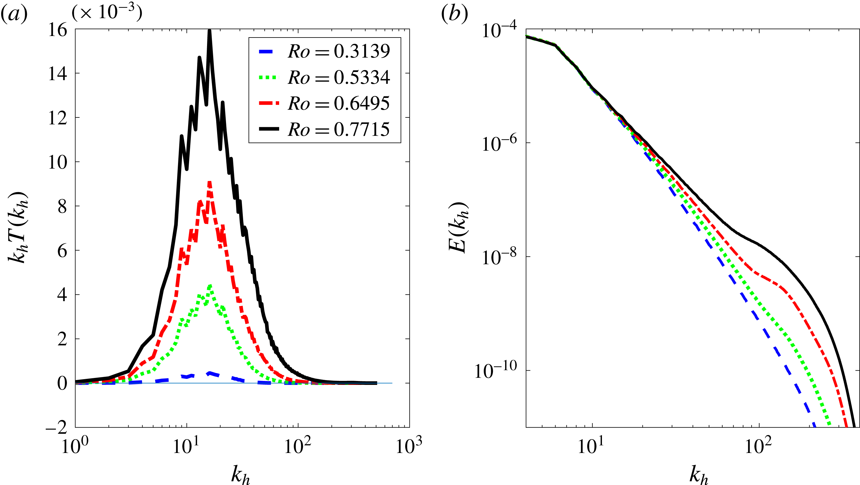
To address this question, we present the spectrum of transfer to imbalance for four different Rossby numbers in figure 5(a). The corresponding energy spectra are also plotted in figure 5(b). The transfer spectra are calculated at the beginning of the integration interval, as the most significant energy transfer takes place early in the simulations. It leads to a shallower tail of
 $E(k_{h})$
later, as shown in figure 5(b). In agreement with previous studies such as those of Nadiga (Reference Nadiga2014) and Kafiabad & Bartello (Reference Kafiabad and Bartello2016), the kink of the energy spectrum changes considerably with
 $Ro$
for these simulations, as does the amplitude of transfer from balanced to unbalanced components. However,
 $T_{U}$
peaks at the same wavenumber (
 $k_{h}\simeq 20$
) for all Rossby numbers. Only the magnitude of the maximum
 $T_{U}$
increases as rotation weakens. This demonstrates that the scale at which the balanced energy flows into the unbalanced motion is invariant to the strength of rotation. This also implies that the breakdown of balance begins in the larger scales where
 $Ro$
and
 $Fr$
are small.
(a) Plots of
 $k_{h}T_{U_{0}}(k_{h})$
divided by
 $Ro^{2}$
. (b) Plots of
 $k_{h}T_{U_{2}}(k_{h})$
divided by
 $Ro^{4.4}$
. Each curve corresponds to the initial Rossby number shown in the legend and all of the spectra are averaged over the interval of
 $[0,0.02\overline{\unicode[STIX]{x1D701}}]$
.

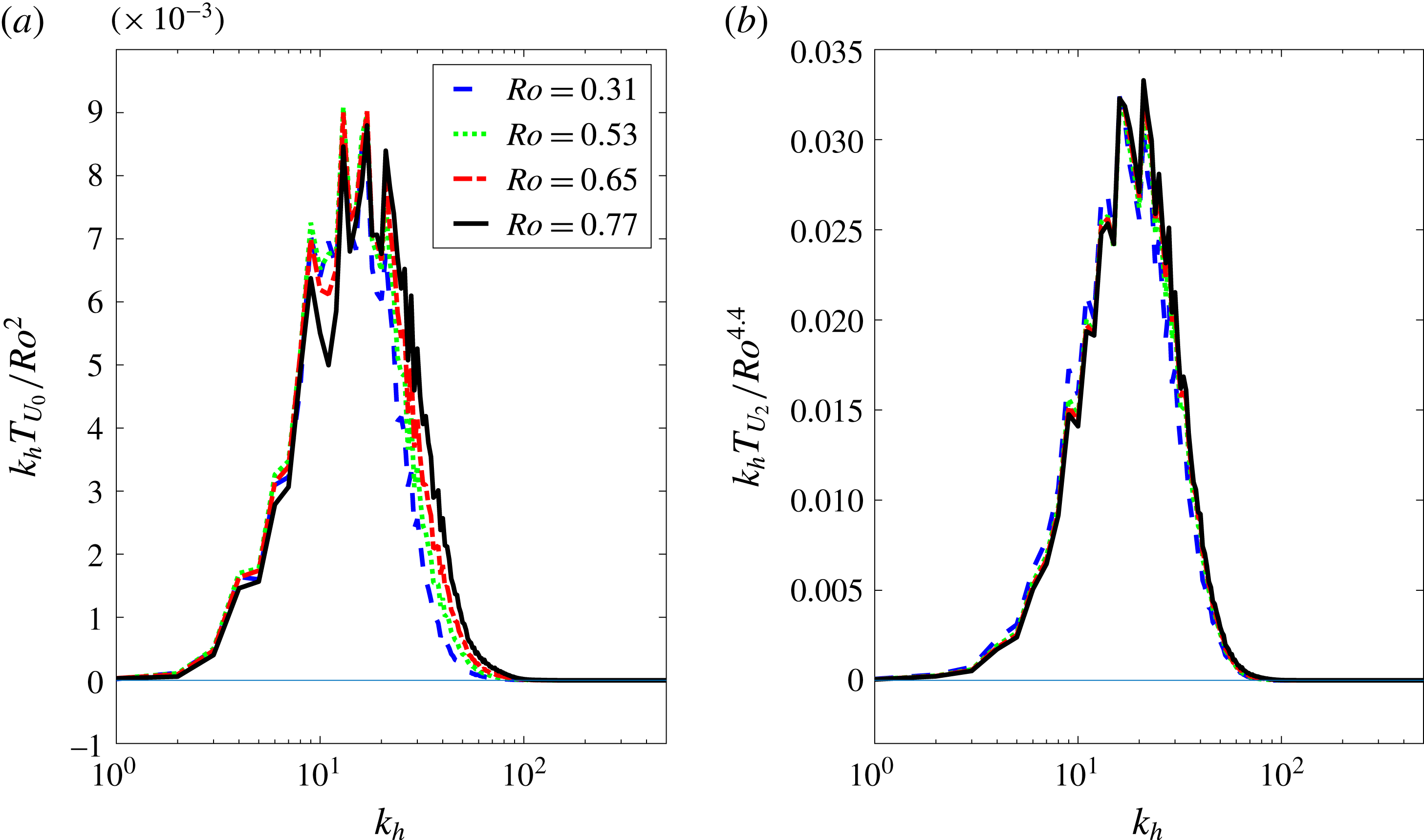
As will be discussed in § 4.6, the unbalanced modes can contain IGWs as well as other dynamics. However, after investigating the frequency spectra of the scales at which
 $T_{U}$
peaks initially (
 $k_{h}\simeq 20$
), we find that the unbalanced modes are predominantly IGWs at these wavenumbers. Therefore, by studying the initial
 $T_{U}$
, we derive how the generated IGWs scale with
 $Ro$
. Figure 6 portrays the unbalanced transfer of four different Rossby numbers scaled with
 $Ro^{n}$
for two different orders of balance, where
 $n$
is the best-fit exponent. Figure 6(a) indicates that the transfer at zeroth order (which is merely transfer to ageostrophic modes) scales with
 $Ro^{2}$
and the transfer at second order scales with
 $Ro^{4.4}$
. Although figure 1 implies that the wavenumber at which
 $T_{U}$
peaks does not change considerably with the order of balance, the results of figure 6 demonstrate that the scaling of its magnitude does change substantially. As will be shown in § 4.6, ageostrophic modes can have a balanced part that behaves like geostrophic modes. Therefore, a substantial part of
 $T_{U_{0}}$
does not display wave-like dynamics. Higher orders of balance such as those shown in figure 6(b) are more indicative of IGW generation. In both panels of this figure, the curves have almost the same profile after scaling. The reason behind the scaling in (b) (
 $Ro^{4.4}$
) is an open question to the authors.
Vanneste & Yavneh (Reference Vanneste and Yavneh2004) presented an example of IGW generation from a particular balanced solution. They showed numerically and analytically that the amplitude of IGWs scales exponentially with the inverse Rossby number. Several other studies, such as those of Vanneste (Reference Vanneste2013) and Nadiga (Reference Nadiga2014), reported similar scalings for low-order dynamics or particular solutions of the primitive equations. Unlike the examples of Vanneste (Reference Vanneste2013), the scaling of
 $T_{U}$
with
 $Ro$
in figure 6 is power law and not exponential. This is mainly because the turbulent flow has a spectrum of scale-dependent
 $Ro$
(and
 $Fr$
) numbers as opposed to one distinct value. Vanneste (Reference Vanneste2013) himself expressed that ‘the power-law wavenumber and frequency spectra of turbulence suggest that the exponential dependence of IGW amplitudes on
 $\unicode[STIX]{x1D716}$
found in smooth flows is replaced by a power-law dependence’. Nadiga (Reference Nadiga2014) studied the evolution of a baroclinic wave in a high-resolution Boussinesq model and observed the exponential scaling as well. His IC had only a limited number of geostrophic modes at zero-order balance (geostrophic thermal-wind balance), whereas ours is a broad distribution that is the output of a QG turbulence simulation at second-order balance.
4.4 The effect of
 $L$

It can be inferred from figure 5 that imbalance generation depends mostly on the larger scales that are predominantly balanced. One of the characteristic parameters of the large-scale dynamics is the wavenumber at which the horizontal energy spectrum peaks, which we denote by
 $L$
. If
 $H$
is defined as the most energetic vertical scale, then
 $L$
is proportional to
 $NH/f$
in these simulations (Charney Reference Charney1949). To derive initial conditions with different
 $L$
, we performed different preliminary QG simulations. These decaying QG simulations started with a distribution of energy proportional to
 $\text{e}^{(k-k_{i})^{2}}$
. Simulations B1536Ki10, B1536Ki20, B1536Ki49 and B1536Ki160 are based on ICs produced by the QG runs with
 $k_{i}=10$
, 20, 49 and 160 respectively. After running the QG models for
 $t=5\overline{\unicode[STIX]{x1D701}}$
, these simulations reached a fully developed state and the peak of the energy spectrum moved towards smaller wavenumbers. Then, we derived the balanced ageostrophic modes associated with the output of the QG simulations and used them as ICs in B1536Ki10, B1536Ki20, B1536Ki49 and B1536Ki160. We adjusted
 $f$
such that the Rossby number based on the initial geostrophic vertical vorticity remained the same (
 $Ro=0.5$
).
The spectra of transfer to imbalance (a), balanced energy (b) and unbalanced energy spectra (c) for simulations B1536Ki10, B1536Ki20, B1536Ki49 and B1536Ki160. The energy spectra are calculated at
 $t=2.5$
eddy turnover times and the transfer spectra at
 $t=0.5$
eddy turnover times. The vertical lines mark the discrete wavenumber at which each curve reaches its maximum.

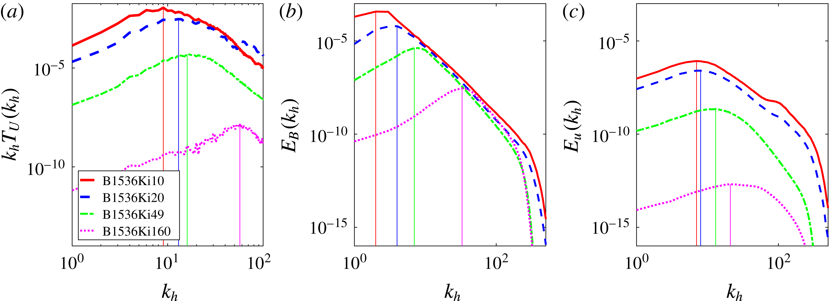
Figure 7(b) portrays
 $E_{B}(k_{h})$
of these simulations. As was the goal, each curve has a peak at a different wavenumber. The initial
 $T_{U}(k_{h})$
depicted in figure 7(a) has the same sequence of peaks as those of the balanced energy. As discussed in § 4.2, the initial
 $T_{U}$
is mostly the transfer from balance to imbalance. Therefore, it can be concluded that by decreasing
 $L$
, the scale at which imbalance is generated decreases as well. For the unbalanced energy spectrum in (c), the maxima occur in the same sequence as those of (a) and (b). Knowing that the unbalanced energy is formed by the initial transfer from the balanced modes, it is expected that figures 7(c) and 7(a) have the same sequence of maxima. Considering the similar sequences of maxima for
 $T_{U}$
,
 $E_{B}$
and
 $E_{U}$
, one may try to quantify how these wavenumbers scale with respect to one another. This is hard to do in our simulations for two reasons. First, the energy spectrum peaks at very low wavenumbers for some of them. Since these wavenumbers are discrete values, the difference between them cannot be measured accurately. Second, we are suspicious of the spurious effect of the box size in B1536Ki10 and B1536Ki20, because the peaks of their energy spectra are close to the scale of the domain. Further investigation of the relationship between the wavenumbers of maximum
 $T_{U}$
,
 $E_{B}$
and
 $E_{U}$
requires the employment of a larger computational domain.
4.5 The effect of
$N/f$

In the simulations that have been presented so far,
 $N/f$
has been kept the same and equal to 8. However, this ratio is measured to be around 30 in the ocean and 100 in the atmosphere. To project the results to higher
 $N/f$
, we present two other sets of simulations with
 $N/f=16$
and 32. The simulations B2048N/f8, B2048N/f16 and B2048N/f32 in table 1 represent
 $N/f=8$
, 16 and 32 respectively. As explained in § 3, the aspect ratio of the domain has to change proportionally to
 $N/f$
to keep the grid points equally spaced. Hence, to produce ICs for each simulation with different
 $N/f$
, different QG simulations are performed. The outputs of these QG simulations have slightly different levels of energy, which leads to a small modification of
 $f$
to keep the Rossby number the same (see table 1). Since
 $f$
is kept similar,
 $N$
changes substantially, leading to a smaller Froude number at higher
 $N/f$
. The nearly geostrophic balanced flow at large scales is characterised by small
 $Ro$
and
 $Fr$
numbers. If
 $Fr$
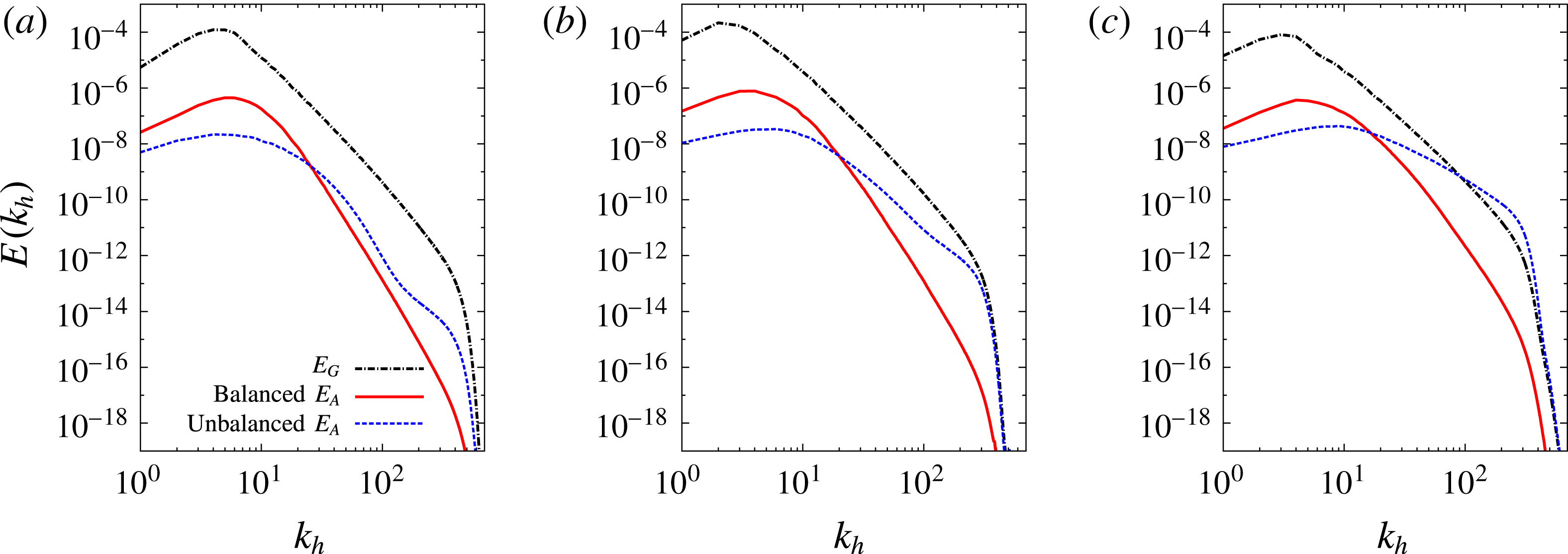
is smaller for a flow, balance is expected to prevail up to smaller scales. Therefore, as shown in figure 8, the shallow tail of the energy spectrum develops at smaller scales when
 $N/f$
is increased.
The energies
 $E_{G}$
,
 $E_{A^{b}}$
and
 $E_{A^{u}}$
at
 $Ro=0.58$
after 27 eddy turnover times for (a)
 $N/f=32$
(resolution
 $2048^{2}\times 64$
), (b)
 $N/f=16$
(resolution
 $2048^{2}\times 128$
) and (c)
 $N/f=8$
(resolution
 $2048^{2}\times 256$
).

4.6 Time scales and frequency spectra
As mentioned in § 2.1, the concept of balance is entwined with the separation of time scales. The filtering of the fast motion in balance dynamics is possible only when there is a considerable disparity between time scales. At smaller scales, the time scale decreases in isotropic turbulence. Therefore, the turbulent time scale changes across length scales. In this section, we study the time scales of balanced and unbalanced modes at different wavenumbers to shed more light on the interaction between them and whether they can be viewed as quasilinear modes.
The normal-mode decomposition that was reviewed in § 2.3 has been extensively used in geophysical fluid dynamics. This decomposition, as explained, is based on the linear part of the equations. The ageostrophic modes defined there are also frequently referred to as wave modes (e.g. Lelong & Riley Reference Lelong and Riley1991; Bühler, Callies & Ferrari Reference Bühler, Callies and Ferrari2014). This is because they exhibit wave dynamics if the nonlinear terms are neglected, not because they have wave-like properties in the fully nonlinear context. This gives rise to the question of the extent to which these modes behave like IGWs. The answer, of course, depends on how small the nonlinear terms are compared with the linear terms in different regimes. The recent applications of normal-mode decomposition to observed data raise the importance of addressing this question. More specifically, Bühler et al. (Reference Bühler, Callies and Ferrari2014) suggested a method to apply the wave–vortex (geostrophic–ageostrophic) decomposition to the one-dimensional spectra of the observed horizontal velocity and buoyancy. They applied their method to aircraft data (Callies, Ferrari & Bühler Reference Callies, Ferrari and Bühler2014; Callies, Bühler & Ferrari Reference Callies, Bühler and Ferrari2016) and concluded that the shallow part of the atmospheric mesoscale spectrum is dominated by IGWs as the energy spectrum of the wave modes exceeds the energy spectrum of the vortical modes in these scales. Without concluding that the mesoscale spectrum is dominated by IGWs, idealised turbulence simulations also reported that linear wave modes have larger amplitudes than vortical modes do in this shallow range (e.g. Bartello Reference Bartello1995, Reference Bartello2010; Deusebio et al.
Reference Deusebio, Vallgren and Lindborg2013). Using the weather research and forecasting (WRF) model, Waite & Snyder (Reference Waite and Snyder2009, Reference Waite and Snyder2013) also investigated the shallow part of the mesoscale spectrum from a turbulence perspective by simulating an idealised baroclinic wave. In their dry simulations, they observed that in the upper troposphere, the rotational energy is much larger than the divergent energy. However, by including moist processes, they reported that the divergent energy increases. Knowing that only wave modes have a divergent part, they expressed that ‘the divergence field in physical space is consistent with IGWs being generated in regions of latent heating’. Lindborg (Reference Lindborg2015) argued that if IGWs prevail, in theory the ratio of rotational to divergent structure functions must be smaller than unity. However, he showed that this ratio was somewhat larger than 1 for the observed data. Hence, he concluded that IGWs cannot be the principal explanation of the shallow mesoscale energy spectrum. In response, Callies et al. (Reference Callies, Bühler and Ferrari2016) mentioned that structure functions suffer from the aliasing of large-scale rotational energy to smaller scales. Therefore, the rotational structure function in the mesoscale can have spuriously large values. Most recently, Asselin et al. (Reference Asselin, Bartello and Straub2018) employed a rapidly varying stratification profile to account for the tropopause in their turbulence simulations. They performed a detailed frequency analysis and concluded that it is unlikely to observe wave-like dynamics in the shallow mesoscale range for the regime of intermediate and high Rossby numbers. However, they reported significant wave activity in the scales larger than the shallow range, where the slope of the spectrum was steep (close to
 $-3$
). In light of these arguments, we found it insightful to thoroughly investigate the frequency spectrum of balanced and unbalanced modes. This analysis can delineate at which scale and to what extent wave-like dynamics are present. Knowing the limitations of our idealised simulations compared with the real ocean and atmosphere, it is hoped that this frequency analysis adds to the picture drawn by the aforementioned studies.
We use horizontal isotropy of the flow to ensure that the frequency spectra of figures 10 and 11 are statistically reliable. In so doing, we save the time series of the complex variables
 $G_{\boldsymbol{k}}$
,
 $A_{\boldsymbol{k}}^{b}$
and
 $A_{\boldsymbol{k}}^{u}$
for all wavenumbers that lie on half-rings (constant
 $k_{h}$
and
 $k_{z}$
, and
 $k_{x}>0$
). The set of
 $\{5,10,25,97,197\}$
is selected for horizontal wavenumbers and marked by vertical lines in figure 9. Then, we take the Fourier transform of these time series and average them over all of the modes with the same
 $k_{h}$
and
 $k_{z}$
. We implement this procedure on the real and imaginary parts of these modes to double the number of samples. This leads to 12 independent modes overall for
 $k_{h}\in \{5,10,97,197\}$
and 20 modes for
 $k_{h}=25$
. For each mode, 9650 points are sampled from
 $t=0$
to
 $t=3.14\overline{\unicode[STIX]{x1D701}}$
, and the Hann window is employed to minimise the spectral leakage due to the non-periodicity of the signals. We carried out our analysis for barotropic modes as well as a baroclinic mode (
 $k_{z}=3\times N/f=24$
), which is marked in the inset of figure 9.
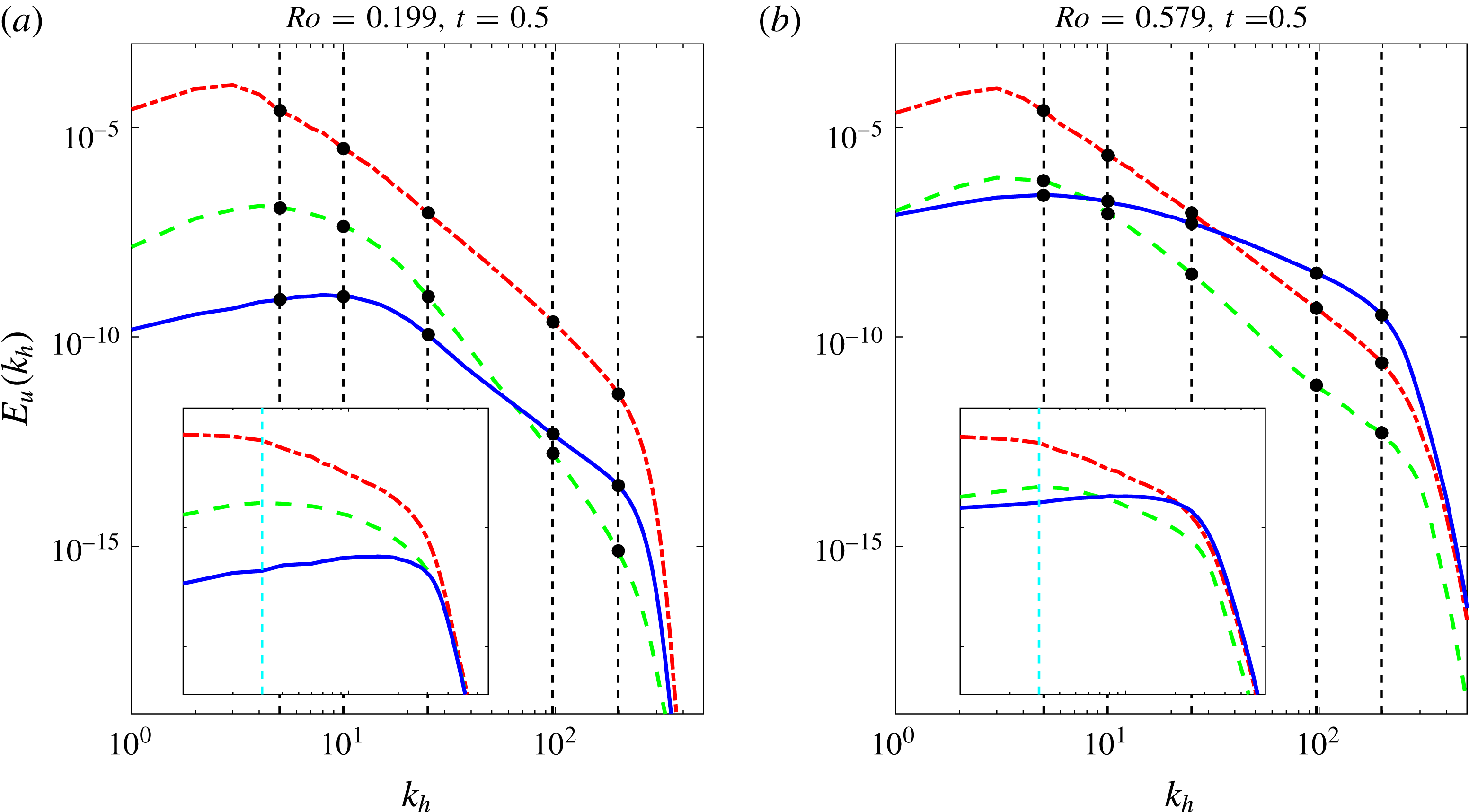
The geostrophic (red dash-dotted curve), balanced ageostrophic (dashed green curves) and unbalanced ageostrophic (sold blue curves) energy spectra of simulations with
 $Ro=0.199$
(a) and
 $Ro=0.579$
(b). The main plots are horizontal energy spectra and the insets are vertical energy spectra. The dashed vertical lines show the set of
 $k_{h}$
and
 $k_{z}$
for which the time series are saved and the frequency spectra are calculated.

We illustrate how the time scales of different regimes of flow change by studying the frequency spectra of two simulations with different Rossby numbers. The energies
 $E_{G}$
,
 $E_{A^{b}}$
and
 $E_{A^{u}}$
of these Rossby numbers are shown in figure 9 to clarify which regime of the flow is analysed. At the low Rossby number,
 $E_{G}$
and
 $E_{A}$
do not cross each other in the resolved range of scales. However,
 $E_{A^{b}}$
and
 $E_{A^{u}}$
cross at
 $k_{h}\simeq 60$
. Below this wavenumber,
 $E_{A^{b}}$
is larger than
 $E_{A^{u}}$
, marking the regime of balance. At
 $Ro=0.579$
,
 $E_{U}$
exceeds
 $E_{B}$
for wavenumbers
 $k_{h}>37$
, which marks the regime that contains imbalance. The inset plots show that the difference between the balanced and unbalanced energies decreases when
 $k_{z}$
is increased from 0 to 24.
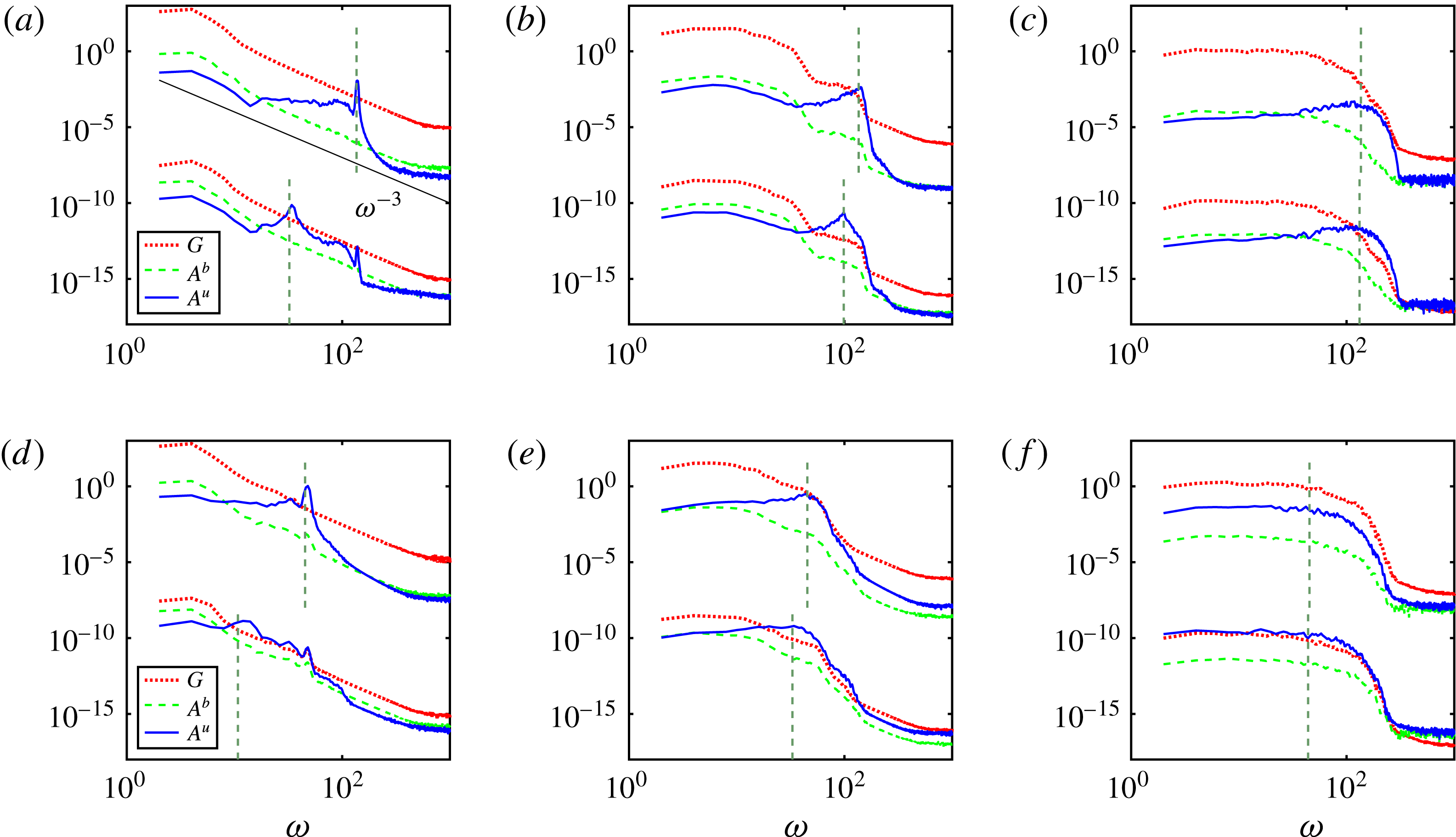
The geostrophic (red dotted), balanced ageostrophic (green dashed) and unbalanced ageostrophic (solid blue) frequency spectra of modes with fixed
 $k_{h}$
and
 $k_{z}$
for (a,d)
 $k_{h}=5$
, (b,e)
 $k_{h}=25$
and (c,f)
 $k_{h}=97$
. The baroclinic modes (
 $k_{z}=24$
) are shifted down (multiplied by
 $10^{-10}$
) for better visualisation. Hence, they lie below the barotropic modes (
 $k_{z}=0$
). (a–c) The simulation with
 $Ro=0.199$
; (d–f) the simulation with
 $Ro=0.579$
. The dashed vertical lines are the linear frequencies.

Figure 10 displays the frequency power spectrum of the geostrophic as well as the balanced and unbalanced ageostrophic modes. Figure 10(a) represents the regime of low
 $k_{h}$
and small Rossby number. At the low frequencies of this panel, the amplitudes of the balanced modes are higher than those of the unbalanced modes. However, close to the linear frequency, the amplitudes of the unbalanced modes exceed those of the balanced modes. Considering that the maximum amplitude of
 $G$
(at low frequencies) is still much larger than the peak of
 $A^{u}$
at
 $\unicode[STIX]{x1D70E}_{\boldsymbol{k}}$
, we expect the wave dynamics to be overshadowed by geostrophic motion in this regime. Excluding the balanced part,
 $A^{u}$
displays a sharp peak at low
 $Ro$
and low
 $k_{h}$
, signalling that the unbalanced motion in this regime behaves like linear IGWs. This is quite expected as the scale-dependent
 $Ro$
is very low at this small wavenumber. Hence, nonlinear interactions are weak. Here,
 $G$
and
 $A^{b}$
show similar behaviour as the balanced ageostrophic modes are approximately slaved to geostrophic modes according to the slave relation (2.6).
The spectra of
 $k_{h}=25$
delineate the role of IGWs in the breakdown of balance. At this wavenumber, the amplitude of
 $A^{u}$
increases more significantly from
 $\unicode[STIX]{x1D714}=36$
to
 $\unicode[STIX]{x1D714}=136$
. Over this range of frequencies, the geostrophic amplitude plateaus. Therefore, unlike the corresponding spectrum at
 $k_{h}=5$
, it is shallower and no longer shows the
 $-3$
slope. This is due to the interaction between the balanced and unbalanced modes at these frequencies and indicates that the geostrophic time scale is being influenced by the wave time scale. This influence leads to further amplification of geostrophic modes close to the linear frequency at
 $k_{h}=97$
. At this wavenumber, the balanced modes have no distinct slow time scale since the geostrophic curve stays rather flat from the very low frequencies to the linear frequency. Knowing that at this
 $Ro$
the total energy spectrum does not display a shallow tail, one can conclude that the separation of time scales breaks at wavenumbers smaller than the kink of the energy spectrum.
By comparing the corresponding results for the two Rossby numbers (panels a–c and d–f of figure 10), we find that the peaks of
 $A^{u}$
at
 $Ro=0.579$
are less sharp but have higher amplitudes. In other words, at higher Rossby numbers, the wave modes are stronger but also interact more with the other modes, and hence behave less linearly. For example, the peak of the barotropic
 $A^{u}$
has an amplitude of 0.012 at
 $Ro=0.199$
and 1.053 at
 $Ro=0.579$
. The former peak is also much spikier than the latter.
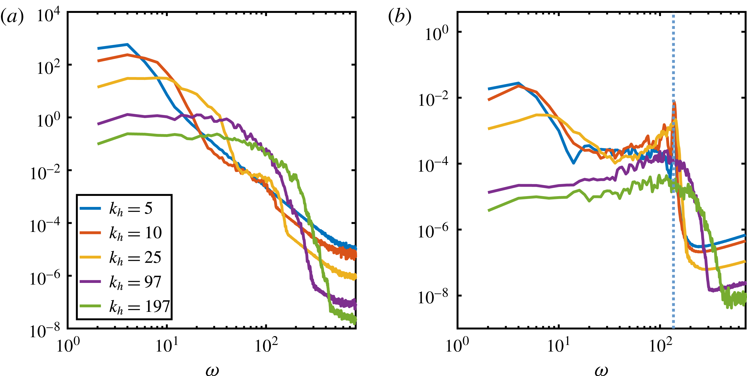
The frequency spectra of the geostrophic (a) and unbalanced ageostrophic (b) modes for
 $k_{h}\in \{5,10,25,97,197\}$
. Here,
 $Ro=0.199$
.

The change of frequency spectra across different scales can better be seen in figure 11, where more horizontal wavenumbers are displayed together. The frequency spectra of geostrophic and ageostrophic modes have been previously studied by Deusebio et al. (Reference Deusebio, Vallgren and Lindborg2013) and Kafiabad & Bartello (Reference Kafiabad and Bartello2017). The former used forcing for geostrophic modes and the latter performed decaying simulations with nonlinearly balanced ICs. Most features of figure 11 qualitatively agree with the results of the aforementioned studies. By increasing
 $k_{h}$
, the peak of
 $A^{u}$
at the linear frequency spreads out to the extent that, at
 $k_{h}=97$
and
 $k_{h}=197$
, there is no distinct peak in the unbalanced frequency spectrum. Hence, it can be concluded that at the shallow range of the energy spectrum, the unbalanced modes do not exhibit wave-like dynamics. At
 $k_{h}=5$
, there is a distinct peak in the geostrophic spectra, which corresponds to the slow geostrophic time scale. However, by increasing
 $k_{h}$
, the geostrophic peaks spread towards higher frequencies. Therefore, these curves become nearly flat over a wide range of frequencies, confirming that the time scale disparity loses its meaning at smaller scales. The other interesting features of the geostrophic curves are the secondary plateaus at
 $k_{h}=10$
and
 $k_{h}=25$
, which appear after a drop from the largest amplitudes. As discussed, these ranges coincide with the peaks of the unbalanced curves close to the linear frequency and reflect the interactions between balanced and unbalanced modes.
Parts of the trends observed across the different scales in figure 11 corroborate the results of Asselin et al. (Reference Asselin, Bartello and Straub2018). These authors also investigated the level of wave amplitude for the unbalanced motions at different wavenumbers. Due to the complications of their geometry and their stratification profile, they could not employ a linear or high-order balance–imbalance decomposition. Instead, they employed high-pass filtering of the superinertial frequencies (
 $\unicode[STIX]{x1D714}>f$
) to derive their high-frequency modes. They examined the time-lagged correlation between the velocity components of these high-pass-filtered modes to investigate the level of wave activity. They concluded that even the unbalanced modes show less and less wave behaviour as
 $k_{h}$
increases.
In figure 10, there is a support around the unbalanced peaks, where the amplitude of
 $A^{u}$
rises and has higher values than the neighbouring frequencies. For instance, this support starts from
 $\unicode[STIX]{x1D714}=14$
ends at
 $\unicode[STIX]{x1D714}=N=136$
in figure 10(a). Although at lower
 $k_{h}$
the peaks are spikier, the supports around them are wider. This is probably due to the disparity between the linear frequencies of the modes with similar
 $k_{h}$
but different
 $k_{z}$
. More specifically, changing
 $k_{z}$
at low
 $k_{h}$
affects the linear frequency more than a similar change at higher
 $k_{h}$
. If we change
 $k_{z}$
from zero to
 $\unicode[STIX]{x0394}k_{z}$
, according to (2.17a,b
), the linear frequency changes from
 $N$
to
 $$\begin{eqnarray}\unicode[STIX]{x1D70E}_{\boldsymbol{k}}^{\ast }=f\sqrt{1+\frac{N^{2}/f^{2}-1}{1+{\unicode[STIX]{x0394}k_{z}}^{2}/k_{h}^{2}}}.\end{eqnarray}$$
If
 ${\unicode[STIX]{x0394}k_{z}}^{2}/k_{h}^{2}$
is small,
 $\unicode[STIX]{x1D70E}_{\boldsymbol{k}}^{\ast }$
stays closer to
 $N$
. Larger values of
 $k_{h}$
keep
 ${\unicode[STIX]{x0394}k_{z}}^{2}/k_{h}^{2}$
small. Hence, the linear frequency gets less affected by changing
 $k_{z}$
at larger
 $k_{h}$
. As a result, in figure 10, the dashed vertical lines of the barotropic and baroclinic modes get closer to one another as
 $k_{h}$
increases. According to the locality assumption, triad interactions are more effective when their wavenumbers are close to each other. If this assumption holds in our simulations, at low
 $k_{h}$
, the local wavenumbers have a wider range of frequencies, and their nonlinear interactions can widen the support around the peak of
 $A^{u}$
. The secondary peaks of the baroclinic modes in figure 10(a,d) may also corroborate the reasoning above, since they occur close to
 $\unicode[STIX]{x1D714}=N$
.
From this analysis, we conclude that spontaneously generated IGWs are observed when (1)
 $Ro$
is large enough that the unbalanced ageostrophic modes are comparable to the balanced geostrophic modes or (2) balance still dominates imbalance such that there is a separation of time scales and nonlinear interactions are not too strong. These opposing conditions mark the regime in which wave dynamics are most sensibly observed. It occurs at atmospheric scales slightly larger than the kink of the energy spectrum, but not too large such that unbalanced motion is overshadowed by balanced dynamics. This range of scales is similar to that at which the maximum transfer between balance and imbalance occurs (discussed in § 4.2). Although the scale range of maximum wave energy is relatively narrow, it plays an important role in the breakdown of balance. This breakdown of balance subsequently leads to the development of shallow spectra at smaller scales. We can also conclude that wave dynamics are more pronounced in large-scale baroclinic modes than barotropic modes since their unbalanced contributions have higher amplitudes.
5 Conclusion
Employing high-order balance, we elaborated on an internal mechanism that transfers energy from the balanced to the unbalanced part of a turbulent rotating stratified flow. This transfer of energy leads to a change of spectral scaling from
 $k_{h}^{-3}$
to
 $k_{h}^{-5/3}$
. This mechanism is summarised in figure 12, where the energy spectra and the ratio of characteristic slow to fast frequencies are schematically portrayed. The total energy spectrum, which is the sum of the balanced and unbalanced energy spectra, has two power-law subranges. The large-scale subrange has a steep slope of
 $-3$
and is dominated by balanced energy. The small-scale subrange, on the other hand, is predominantly unbalanced and displays a shallow slope of
 $-5/3$
(see Kafiabad & Bartello Reference Kafiabad and Bartello2016, Reference Kafiabad and Bartello2017). At the small-scale end of the steeper subrange, the balanced energy leaks into the unbalanced motion. The wavenumber at which the maximum transfer from balance to imbalance occurs is marked by
 $k_{B\rightarrow U}$
in figure 12. We showed that
 $k_{B\rightarrow U}$
is slightly larger than the peak of the balanced energy spectrum, indicating that balance breaks down at scales where the energy spectrum is still steep. This fact stems from the decreasing of the difference between the fast and slow time scales which starts at these scales according to our frequency analysis. As shown in figure 12, the ratio of characteristic slow to fast frequencies is equal to
 $Ro$
at small wavenumbers and starts to increase at a wavenumber larger than
 $k_{B\rightarrow U}$
. Therefore, there is a range of wavenumbers larger than
 $k_{B\rightarrow U}$
where the separation of time scales is somewhat maintained. This range of wavenumbers is marked as imbalance generation in figure 12 and has several characteristics. First, the fast frequency is approximately equal to the linear frequency of IGWs in this range, according to our frequency analysis in § 4.6. Hence, one may conclude that the leaked balanced energy is mostly transferred to IGWs, and they play an important role in the onset of balance breakdown. Second, once the IGWs are generated, resonant catalytic interactions probably enhance the forward cascade of energy in this range. In a resonant catalytic interaction, a balanced mode facilitates the transfer of energy between two opposite-signed unbalanced modes and remains unchanged, as described by Bartello (Reference Bartello1995). In the range of Rossby numbers investigated in this study,
 $k_{B\rightarrow U}$
is found to be dependent on the characteristic horizontal scale but invariant to a change of Rossby number. Unlike this wavenumber, the flux of energy from balance to imbalance (marked by
 $\unicode[STIX]{x1D716}_{u}$
in figure 12) depends sensitively on
 $Ro$
(as also reported by Vallgren et al.
Reference Vallgren, Deusebio and Lindborg2011). This flux is directed towards smaller scales and forms a power-law scaling of
 $k_{h}^{-5/3}$
.
The schematic picture of the break in spectral scaling due to the breakdown of balance.

At very small scales, in addition to the unbalanced spectrum, the tail of the balanced spectrum becomes shallow as well, confirming previous studies such as those of Bartello (Reference Bartello2010), Deusebio et al. (Reference Deusebio, Vallgren and Lindborg2013) and Kafiabad & Bartello (Reference Kafiabad and Bartello2016). At these scales, the balanced and unbalanced modes exchange energy, as the fast and slow time scales become the same. Consequently, the distinction between balance and imbalance breaks down completely and the flow becomes weakly rotating stratified turbulence. Therefore, the energy tends to equipartition among different modes, with
 $k_{h}^{-5/3}$
scaling eventually leading to stratified turbulence (e.g. see Billant & Chomaz Reference Billant and Chomaz2001; Lindborg Reference Lindborg2006; Bartello & Tobias Reference Bartello and Tobias2013). There is a transition range of wavenumbers marked in figure 12 where the difference between the fast and slow time scales decreases until they merge into a single turbulent time scale. In this range, the unbalanced modes show less and less wave-like behaviour and their nonlinear interactions with one another increase.
There have been previous studies relying on linear balance to decompose rotating stratified flows to a set of geostrophic and ageostrophic modes (Bartello Reference Bartello1995; Ngan et al.
Reference Ngan, Bartello and Straub2008; Bartello Reference Bartello2010; Deusebio et al.
Reference Deusebio, Vallgren and Lindborg2013). Some of the ageostrophic motion is slowly varying and slaved to the geostrophic modes, which cannot participate in a down-scale cascade. The rest of the ageostrophic motion has high frequencies and contributes to energy, but not potential enstrophy, at low
 $Ro$
and
 $Fr$
. In the latter case, a down-scale cascade via the catalytic interaction is the inevitable result, according to the arguments presented in Bartello (Reference Bartello1995). In this study, we extended the balance–imbalance decomposition to higher orders to show how the relative mix of these two components is distributed in wavenumber, and how they vary with the Rossby number. We found that both linear and nonlinear balance decompositions yield the shallow small-scale range in the energy spectrum. However, the source of this energy is in the large scales where the difference between linear and nonlinear balance can be substantial. Some of these differences are listed below.
(i) The most important difference between the generated ageostrophic energy and spontaneous imbalance is their scaling with
$Ro$
. Ageostrophic energy scales with
$Ro^{2}$
, whereas the scaling exponent is larger than 2 for spontaneous imbalance. At second-order balance, we found this exponent to be approximately 4.4. The spontaneous generation of IGWs in low-order dynamical systems or special solutions of the fluid equations has been shown to scale inverse-exponentially with
$Ro$
(Vanneste & Yavneh Reference Vanneste and Yavneh2004; Nadiga Reference Nadiga2014). We, on the other hand, simulated turbulent balanced flows and considered imbalance generation in a broader sense. For these reasons, the exponential dependence of IGWs on
$Ro$
was replaced by power-law dependence in our simulations, as speculated by Vanneste (Reference Vanneste2013). While we covered only a limited range of Rossby numbers (from
$Ro=0.3$
to
$Ro=0.8$
), consideration of a broader range of Rossby numbers could make the scaling cleaner.(ii) The energy transfer from geostrophic to ageostrophic modes reported by linear balance is higher than the energy transfer from balance to imbalance reported by high-order balance. This is because a part of geostrophic energy is transferred to balanced ageostrophic modes, which is rightly not accounted for in the transfer to imbalance at higher orders.
(iii) High-order balance displays a small kink in the ageostrophic energy spectrum, which is steep at low wavenumbers. Kafiabad & Bartello (Reference Kafiabad and Bartello2016) showed that the steep part of the ageostrophic energy spectrum is associated with balance and the shallow part with imbalance. GCM studies such as those Hamilton, Takahashi & Ohfuchi (Reference Hamilton, Takahashi and Ohfuchi2008) and Evans et al. (Reference Evans, Lauritzen, Mishra, Neale, Taylor and Tribbia2013) reported that the divergent energy spectra display a kink as well, consistent with the likelihood that the large-scale dynamics of these models are nonlinearly balanced.
(iv) Imbalance generation takes place at early times. However, at later times, as the Rossby number decays, the transfer between balance and imbalance reduces substantially. This transfer is less negligible for linear balance than high-order balance, which indicates that the flow adjusts to a new high-order state of balance.


It should be noted that the method employed for calculating spontaneous imbalance is justified if the flow is predominantly balanced. More particularly, the slave relation (2.6) is required to be a valid approximation. In hindsight, our results show that spontaneous imbalance occurs at scales where the scale-dependent
 $Fr$
and
 $Ro$
are low and the total energy spectrum is steep. Therefore, in this regime, the flow is predominantly balanced. Moreover, it was observed that, starting from an initially balanced condition, imbalance is mostly generated at early times, when the unbalanced shallow tail has not yet developed.
It is hoped that our study can be employed to formulate subgrid parametrisation schemes that judiciously remove balanced energy and dissipate it without necessarily resolving the small-scale unbalanced dynamics. Moreover, our results can be used to determine the resolution that realistic models require to reliably describe large-scale atmospheric and oceanic dynamics.
The break of spectral scaling portrayed in this study is consistent with atmospheric observations (Nastrom & Gage Reference Nastrom and Gage1985; Lindborg Reference Lindborg1999). Nevertheless, several atmospheric phenomena are missing in our idealised simulations. Among these are the presence of external and internal boundaries (tropopause and topography) and convective processes. Hence, we cautiously avoid interpreting the results as the sole explanation of the mesoscale spectral scaling. Yet, the internal mechanism that was delineated here may be part of the explanation for the shallowing of the atmospheric (and the oceanic) spectrum. A different hypothesis was proposed by Gage (Reference Gage1979) and expanded by Lilly (Reference Lilly1983) to explain the
 $k^{-5/3}$
scaling of the mesoscale. This hypothesis attributes the slope of the energy spectrum at mesoscales to the upscale (inverse) cascade of energy in quasi-2D stratified turbulence. The source of this energy was associated with small-scale convective processes by Lilly (Reference Lilly1983). By contrast with this inverse-cascade scenario, we supported the hypothesis of a forward cascade of energy via unbalanced ageostrophic modes (see Lindborg Reference Lindborg2005, Reference Lindborg2006; Brethouwer et al.
Reference Brethouwer, Billant, Lindborg and Chomaz2007; Vallgren et al.
Reference Vallgren, Deusebio and Lindborg2011). Mesoscale meteorologists emphasise the necessity to consider convective sources, which may contribute to the scaling of the mesoscale energy spectrum concurrently (see, e.g., Sun, Rotunno & Zhang Reference Sun, Rotunno and Zhang2017). However, their comparative significance is not clear. As future work, properly designed simulations can include the effects of both the forward cascade of energy that is leaked from large-scale balance dynamics and the convective injection of unbalanced energy at smaller scales. GCM studies, which more realistically model large-scale balance dynamics, cannot resolve the convective scales. Hence, they rely on parametrisation schemes to include these processes (e.g. Hamilton et al.
Reference Hamilton, Takahashi and Ohfuchi2008). On the other hand, mesoscale models, which better resolve the convective scales, cannot extend their large scales to synoptic scales to properly include balance dynamics. Therefore, idealised simulations might be more suitable to incorporate both balance dynamics and convective forcing in one simulation.
Appendix A. Second-order balance
To demonstrate this procedure, we decompose the right-hand side of (2.4) into three parts,
 $\boldsymbol{N}_{\boldsymbol{s}}(\boldsymbol{s},\boldsymbol{f})=\unicode[STIX]{x1D701}_{ss}(\boldsymbol{s})+\unicode[STIX]{x1D701}_{sf}(\boldsymbol{s},\boldsymbol{f})+\unicode[STIX]{x1D701}_{ff}(\boldsymbol{f})$
, where
 $$\begin{eqnarray}\unicode[STIX]{x1D701}_{ss}(\boldsymbol{s})=\boldsymbol{N}_{\boldsymbol{s}}(\boldsymbol{s},0),\quad \unicode[STIX]{x1D701}_{ff}(\boldsymbol{f})=\boldsymbol{N}_{\boldsymbol{s}}(0,\boldsymbol{f}),\quad \unicode[STIX]{x1D701}_{sf}(\boldsymbol{s},\boldsymbol{f})=\boldsymbol{N}_{\boldsymbol{s}}(\boldsymbol{s},\boldsymbol{f})-\unicode[STIX]{x1D701}_{ss}(\boldsymbol{s})-\unicode[STIX]{x1D701}_{ff}(\boldsymbol{f}).\end{eqnarray}$$
Similarly, we can write
 $$\begin{eqnarray}\boldsymbol{N}_{\boldsymbol{f}}(\boldsymbol{s},\boldsymbol{f})=\unicode[STIX]{x1D702}_{ss}(\boldsymbol{s})+\unicode[STIX]{x1D702}_{sf}(\boldsymbol{s},\boldsymbol{f})+\unicode[STIX]{x1D702}_{ff}(\boldsymbol{f}).\end{eqnarray}$$
Expansion of (2.4b
) at
 $O(\unicode[STIX]{x1D716}^{2})$
leads to
 $$\begin{eqnarray}\unicode[STIX]{x1D716}\frac{\unicode[STIX]{x2202}\unicode[STIX]{x1D716}\unicode[STIX]{x1D6FC}^{\prime }}{\unicode[STIX]{x2202}T}+\unicode[STIX]{x1D6E4}\unicode[STIX]{x1D716}^{2}\unicode[STIX]{x1D6FC}^{\prime \prime }=\unicode[STIX]{x1D716}\unicode[STIX]{x1D702}_{\boldsymbol{ s}\boldsymbol{f}}(\boldsymbol{s},\unicode[STIX]{x1D716}\unicode[STIX]{x1D6FC}^{\prime })=\unicode[STIX]{x1D716}^{2}\unicode[STIX]{x1D702}_{\boldsymbol{s}\boldsymbol{f}}(\boldsymbol{s},\unicode[STIX]{x1D6FC}^{\prime }).\end{eqnarray}$$
Therefore,
 $$\begin{eqnarray}\unicode[STIX]{x1D6FC}^{\prime \prime }=\unicode[STIX]{x1D6E4}^{-1}\left[\unicode[STIX]{x1D702}_{\boldsymbol{s}\boldsymbol{f}}(\boldsymbol{s},\unicode[STIX]{x1D6FC}^{\prime })-\frac{\unicode[STIX]{x2202}\unicode[STIX]{x1D6FC}^{\prime }}{\unicode[STIX]{x2202}T}\right],\end{eqnarray}$$
in which
 $\unicode[STIX]{x1D6FC}^{\prime }$
is derived from (2.8). We need an expression for
 $\unicode[STIX]{x2202}\unicode[STIX]{x1D6FC}^{\prime }/\unicode[STIX]{x2202}T$
to complete (A 4). In so doing, we take the slow-time derivate of (2.8),
 $$\begin{eqnarray}\displaystyle \frac{\unicode[STIX]{x2202}\unicode[STIX]{x1D6FC}^{\prime }}{\unicode[STIX]{x2202}T} & = & \displaystyle \unicode[STIX]{x1D6E4}^{-1}\frac{\unicode[STIX]{x2202}}{\unicode[STIX]{x2202}T}\unicode[STIX]{x1D702}_{\boldsymbol{s}\boldsymbol{s}}(\boldsymbol{s})=\unicode[STIX]{x1D6E4}^{-1}\left[\unicode[STIX]{x1D702}_{\boldsymbol{s}\boldsymbol{s}}\left(\boldsymbol{s}+\frac{\unicode[STIX]{x2202}\boldsymbol{s}}{\unicode[STIX]{x2202}T}\right)-\unicode[STIX]{x1D702}_{\boldsymbol{s}\boldsymbol{s}}(\boldsymbol{s})-\unicode[STIX]{x1D702}_{\boldsymbol{s}\boldsymbol{s}}\left(\frac{\unicode[STIX]{x2202}\boldsymbol{s}}{\unicode[STIX]{x2202}T}\right)\right]\nonumber\\ \displaystyle & = & \displaystyle \unicode[STIX]{x1D6E4}^{-1}[\unicode[STIX]{x1D702}_{\boldsymbol{s}\boldsymbol{s}}(\boldsymbol{s}+\unicode[STIX]{x1D701}_{\boldsymbol{s}\boldsymbol{s}}(\boldsymbol{s}))-\unicode[STIX]{x1D702}_{\boldsymbol{s}\boldsymbol{s}}(\boldsymbol{s})-\unicode[STIX]{x1D702}_{\boldsymbol{s}\boldsymbol{s}}(\unicode[STIX]{x1D701}_{\boldsymbol{s}\boldsymbol{s}}(\boldsymbol{s}))].\end{eqnarray}$$
Appendix B. Interaction with imbalance at second order
As shown in § 2.2,
 $\unicode[STIX]{x2202}\boldsymbol{f}^{b}/\unicode[STIX]{x2202}t$
in the context of full dynamics can be derived from (2.11). However, calculation of
 $\unicode[STIX]{x2202}\boldsymbol{H}/\unicode[STIX]{x2202}\boldsymbol{s}$
explicitly might be tedious for high-order balance models. Instead, we derive
 $\unicode[STIX]{x2202}\boldsymbol{f}^{b}/\unicode[STIX]{x2202}t$
according to the balance model and use
 $\unicode[STIX]{x2202}\boldsymbol{s}/\unicode[STIX]{x2202}t$
(derived from (2.10a
)) whenever
 $\unicode[STIX]{x2202}\boldsymbol{s}/\unicode[STIX]{x2202}T$
needs to be calculated. Here, we simplify the notation by using
 $\boldsymbol{N}_{\boldsymbol{s}}$
and
 $\boldsymbol{M}$
for
 $\boldsymbol{N}_{\boldsymbol{s}}(\boldsymbol{s},\boldsymbol{f}^{b}+\boldsymbol{f}^{u})$
and
 $\boldsymbol{M}(\boldsymbol{s},\boldsymbol{f}^{b}+\boldsymbol{f}^{u})$
respectively. The time derivative of (2.7) yields
 $$\begin{eqnarray}\frac{\unicode[STIX]{x2202}\boldsymbol{f}^{b}}{\unicode[STIX]{x2202}t}=\frac{\unicode[STIX]{x2202}\unicode[STIX]{x1D6FC}}{\unicode[STIX]{x2202}t}+\unicode[STIX]{x1D716}\frac{\unicode[STIX]{x2202}\unicode[STIX]{x1D6FC}^{\prime }}{\unicode[STIX]{x2202}t}+\unicode[STIX]{x1D716}^{2}\frac{\unicode[STIX]{x2202}\unicode[STIX]{x1D6FC}^{\prime \prime }}{\unicode[STIX]{x2202}t}+O(\unicode[STIX]{x1D716}^{3}).\end{eqnarray}$$
We already showed that
 $\unicode[STIX]{x1D6FC}=0$
and derived an expression for
 $\unicode[STIX]{x2202}\unicode[STIX]{x1D6FC}^{\prime }/\unicode[STIX]{x2202}t$
in (2.14). For the next-order correction, we first use the balance relation at second order (A 4) to derive
 $$\begin{eqnarray}\unicode[STIX]{x1D716}^{2}\unicode[STIX]{x1D6FC}^{\prime \prime }=\unicode[STIX]{x1D6E4}^{-1}\unicode[STIX]{x1D716}\left[\unicode[STIX]{x1D702}_{\boldsymbol{s}\boldsymbol{f}}(\boldsymbol{s},\unicode[STIX]{x1D716}\unicode[STIX]{x1D6FC}^{\prime })-\frac{\unicode[STIX]{x2202}\unicode[STIX]{x1D6FC}^{\prime }}{\unicode[STIX]{x2202}t}\right]=\unicode[STIX]{x1D6E4}^{-1}\unicode[STIX]{x1D716}[\unicode[STIX]{x1D702}_{\boldsymbol{ s}\boldsymbol{f}}(\boldsymbol{s},\unicode[STIX]{x1D716}\unicode[STIX]{x1D6FC}^{\prime })-\boldsymbol{M}],\end{eqnarray}$$
where (2.14) is used to substitute for
 $\unicode[STIX]{x2202}\unicode[STIX]{x1D6FC}^{\prime }/\unicode[STIX]{x2202}t$
. Next, we take the time derivative of (B 2),
 $$\begin{eqnarray}\displaystyle \unicode[STIX]{x1D716}^{2}\frac{\unicode[STIX]{x2202}\unicode[STIX]{x1D6FC}^{\prime \prime }}{\unicode[STIX]{x2202}t} & = & \displaystyle \unicode[STIX]{x1D6E4}^{-1}\unicode[STIX]{x1D716}\left[\unicode[STIX]{x1D702}_{\boldsymbol{s}\boldsymbol{f}}\left(\frac{\unicode[STIX]{x2202}\boldsymbol{s}}{\unicode[STIX]{x2202}t},\unicode[STIX]{x1D716}\unicode[STIX]{x1D6FC}^{\prime }\right)+\unicode[STIX]{x1D702}_{\boldsymbol{ s}\boldsymbol{f}}\left(\boldsymbol{s},\frac{\unicode[STIX]{x2202}\unicode[STIX]{x1D716}\unicode[STIX]{x1D6FC}^{\prime }}{\unicode[STIX]{x2202}t}\right)-\frac{\unicode[STIX]{x2202}\boldsymbol{M}}{\unicode[STIX]{x2202}t}\right]\nonumber\\ \displaystyle & = & \displaystyle \unicode[STIX]{x1D6E4}^{-1}\unicode[STIX]{x1D716}\left[\unicode[STIX]{x1D702}_{\boldsymbol{s}\boldsymbol{f}}(\unicode[STIX]{x1D716}\boldsymbol{N}_{\boldsymbol{s}},\unicode[STIX]{x1D716}\unicode[STIX]{x1D6FC}^{\prime })+\unicode[STIX]{x1D702}_{\boldsymbol{s}\boldsymbol{f}}(\boldsymbol{s},\unicode[STIX]{x1D716}\boldsymbol{M})-\frac{\unicode[STIX]{x2202}\boldsymbol{M}}{\unicode[STIX]{x2202}t}\right],\end{eqnarray}$$
where
 $\unicode[STIX]{x2202}\boldsymbol{M}/\unicode[STIX]{x2202}t$
can be calculated by taking the time derivative of (2.14) as follows:
 $$\begin{eqnarray}\frac{\unicode[STIX]{x2202}\boldsymbol{M}}{\unicode[STIX]{x2202}t}=\unicode[STIX]{x1D6E4}^{-1}\unicode[STIX]{x1D716}\left[\unicode[STIX]{x1D702}_{ss}\left(\boldsymbol{N}_{\boldsymbol{s}}+\frac{\unicode[STIX]{x2202}\boldsymbol{N}_{\boldsymbol{s}}}{\unicode[STIX]{x2202}t}\right)-\unicode[STIX]{x1D702}_{ss}(\boldsymbol{N}_{\boldsymbol{s}})-\unicode[STIX]{x1D702}_{ss}\left(\frac{\unicode[STIX]{x2202}\boldsymbol{N}_{\boldsymbol{s}}}{\unicode[STIX]{x2202}t}\right)\right].\end{eqnarray}$$