1. Introduction
Modelling of the macroscopic behaviour of a medium that contains microscopic details such as flow in the vicinity of a porous surface (microstructure) that exhibits rapidly varying properties associated with the heterogeneity of the medium has become one of the long-standing sources of challenging problems for mathematical analysis. This requires understanding of the transport phenomena that account for coupled motion between a free-fluid region and a porous medium saturated by the same fluid as well as description of the transitional region at a fluid–porous dividing surface/inter-region responsible for mass and momentum transfer. This poses a great numerical challenge since it involves point-wise computation of flow and pressure fields in the vicinity of the surface micro-structures. The necessity for addressing this problem stems not only from the significant influence exerted by the presence of small-scale surface inhomogeneities at the interface on the transport phenomena, but also from its ubiquitous occurrence in nature and in many industrial and environmental applications (see, e.g. Alazmi & Vafai Reference Alazmi and Vafai2001; Gavrilov et al. Reference Gavrilov, Accary, Morvan, Lyubimov, Méradji and Bessonov2011; Lyubimova et al. Reference Lyubimova, Lepikhin, Parshakova and Tiunov2016; Bottaro Reference Bottaro2019; Angot et al. Reference Angot, Goyeau and Ochoa-Tapia2021).
From a macroscopic perspective, where the concept of surface/interface is related to the average representation, the fluid flow in a coupled flow system and the behaviour at the interface have been characterised by two modelling approaches, the one-domain approach (ODA) and the two-domain approach (TDA). The mesoscopic description (ODA) is based on local volume-averaged equations which are assumed to be valid throughout the domain; a diffuse interface layer of thickness
 $\delta$
larger than the microscopic length scale
 $\ell$
(with
 $\ell \ll l$
, where
 $l$
characterises a macroscopic length scale) appears and the ODA requires prior knowledge of effective properties (permeability, porosity etc.) that vary as the dividing surface is crossed.
The ODA considers the system as a continuum, where the geometrical properties (porosity, permeability) and transport phenomena display rapid spatial changes in the inter-region (Goharzadeh et al. Reference Goharzadeh, Khalili and Jørgensen2005; Valdés-Parada et al. Reference Valdés-Parada, Goyeau and Ochoa-Tapia2007b ; Morad & Khalili Reference Morad and Khalili2009; Terzis et al. Reference Terzis, Zarikos, Weishaupt, Yang, Chu, Helmig and Weigand2019; Valdés-Parada & Lasseux Reference Valdés-Parada and Lasseux2021), regarded as a thin transition porous layer (see figure 1). Ochoa-Tapia & Whitaker (Reference Ochoa-Tapia and Whitaker1995) were among the earliest researchers who presented generalised transport equations (GTE), valid everywhere in the entire system. It is worth mentioning that the ODA comes from a penalisation approach as suggested by Caltagirone & Arquis (Reference Caltagirone and Arquis1986), during the 1980s and a very simple form of the ODA has been proposed by Valdés-Parada & Lasseux (Reference Valdés-Parada and Lasseux2021) which has a Darcy structure with position-dependent coefficients and does not require the inclusion of any Brinkman terms. The subsequent efforts to fulfil the above requirements are based on GTE formulations, free of length constraints, and account for porosity variations by including first and second Brinkman correction terms (Valdés-Parada et al. Reference Valdés-Parada, Alberto Ochoa-Tapia and Alvarez-Ramirez2007a ). Hernandez-Rodriguez et al. (Reference Hernandez-Rodriguez, Angot, Goyeau and Ochoa-Tapia2022) have presented a momentum GTE, valid everywhere in the system and expressed in terms of position-dependent effective medium coefficients, containing the two Brinkman corrective terms along with the Darcy term. The ODA predictions compare well with the results generated by averaging the local profiles resulting from pore-scale simulations. They have predicted the position-dependent permeability tensor from both pore-scale simulations (PSS) and the solution of the corresponding local closure problem in a typical domain of the fluid–porous medium boundary. Their analysis reveals that including the first and the second Brinkman correction terms, along with the position-dependent intrinsic permeability tensor in the Darcy term in the GTE for momentum transport, facilitates accurate predictions of the average velocity profiles of parallel flows everywhere in the system.
It is important to note that the formulation proposed by Valdés-Parada et al. (Reference Valdés-Parada, Alberto Ochoa-Tapia and Alvarez-Ramirez2007a
) is based on a length scale referred to as the Brinkman boundary-layer thickness, which corresponds to the distance across which there is a drastic decrease in velocity at the surface of the porous medium to the Darcy seepage velocity. Note that there are situations when this length scale (
 $\unicode{x1D6E5} _B$
) deviates from the length scale (
 $\delta _B$
) below which the Brinkman diffusion terms are dominant in the bulk of the porous medium. In that case, there can only be a weak influence of the Brinkman correction terms on the base velocity profile. Further, the predictions obtained by Hernandez-Rodriguez et al. (Reference Hernandez-Rodriguez, Angot, Goyeau and Ochoa-Tapia2022) from the modelling of the permeability distribution within the interfacial region (ODA) demonstrate a strong dependence on the size of the averaging volume (
 $r_0$
), discontinuity in the gradient of permeability
 $\kappa$
at the porous side and discontinuity of
 $1/\kappa$
at the fluid end of the transition layer and weak variation in the upper portion of the interfacial region. Besides, it is important that the choice of the permeability distribution in the interfacial region ensures that the averaged velocity distribution in the fluid region remains independent of the size of the averaging volume, as can be observed from the PSS performed by Valdés-Parada & Lasseux (Reference Valdés-Parada and Lasseux2021).
This suggests that one needs to address the following questions pertaining to the inclusion of Brinkman correction terms and the selection of the ODA permeability distribution for accurate and reliable ODA predictions that match well with PSS and experiments: (i) For which situations does one need to include the second Brinkman correction terms in the momentum GTE in the ODA? (ii) How is the Brinkman boundary-layer thickness
 $\unicode{x1D6E5} _B$
related to the size of the averaging volume
 $r_0$
in the homogenisation method? (iii) What should be the choice of the ODA permeability distribution that would ensure agreement of the ODA predicted velocity profiles with the averaged solution of the PSS? It is proposed to address these considerations along with other issues (elaborated below) that are related to modelling appropriate boundary conditions at a porous–fluid interface and propose a predictive model for two-dimensional flows, in the present study.
The TDA considers the porous medium–fluid region as two continuous regions separated by a dividing surface (see figure 1). When
 $\ell \ll l$
, the solution technique comprises describing the micro-scale average behaviour by means of effective surface models, which replace the heterogeneous boundary by a smooth surface on which effective boundary conditions are prescribed. It is crucial to examine the general form of the admissible boundary conditions from a mathematical point of view, given the models in the fluid and the porous regions. It is also important to characterise the transfer in the transition region (mass, momentum) and to model these by appropriate boundary conditions.
In the case of flows over porous media, the development of boundary conditions has been revisited since the empirical condition of Beavers & Joseph (Reference Beavers and Joseph1967), through different up-scaling methods such as the volume-averaging approach (Goyeau et al. Reference Goyeau, Lhuillier, Gobin and Velarde2003), matched asymptotic expansions (Chandesris & Jamet Reference Chandesris and Jamet2006) and multi-scale asymptotic homogenisation (Auriault et al. Reference Auriault, Boutin and Geindreau2009; Jäger & Mikelić Reference Jäger and Mikelić2009). Different models for the fluid and the porous medium scales have been implemented and matched through the corresponding developed jump conditions at the dividing surface (Wood et al. Reference Wood, Quintard and Whitaker2000; Valdés-Parada et al. Reference Valdés-Parada, Goyeau and Alberto Ochoa-Tapia2006). The solution of the associated closure problems has supplied the coefficients involved in the jump conditions. There have been continued efforts in proposing adequate boundary conditions at the interface of the two domains, but there are certain features of the momentum and the mass transport phenomena that have not been accounted for, resulting in some failure to capture significant physical characteristics of the porous surface. These efforts have revealed that the derivation of the boundary conditions must incorporate a direct correlation between the microscopic geometrical details of the porous medium and the corresponding macroscopic transport of mass and momentum; this being a complicated effort in such multi-scale problems, an effective approach has been proposed to capture the averaged effect of the micro-scale characteristics on the macroscopic processes within the framework of TDA. This corresponds to imposing the boundary conditions at a fictive interface between the free fluid and the porous region. Note that the jump boundary conditions are a result of the integration of the momentum transport over a thin transition layer of the ODA (Goyeau et al. Reference Goyeau, Lhuillier, Gobin and Velarde2003; Valdés-Parada et al. Reference Valdés-Parada, Aguilar-Madera, Ochoa-Tapia and Goyeau2013). The derived jump boundary conditions based on the combination of the ODA and the TDA have either assumed the volume-averaging method (Ochoa-Tapia & Whitaker Reference Ochoa-Tapia and Whitaker1995), or are based on the solution of an ancillary closure problem related to macroscopic deviations (Valdés-Parada et al. Reference Valdés-Parada, Aguilar-Madera, Ochoa-Tapia and Goyeau2013) or used matched asymptotic expansion (Chandesris & Jamet Reference Chandesris and Jamet2009) or asymptotic analysis (Angot et al. Reference Angot, Goyeau and Ochoa-Tapia2017).
Valdés-Parada et al. (Reference Valdés-Parada, Aguilar-Madera, Ochoa-Tapia and Goyeau2013) have derived jump boundary conditions for one-dimensional momentum transport in a system composed of a porous medium and a fluid under a constant pressure gradient. These boundary conditions involve a jump in both the velocity and the viscous stress and are presented in terms of the jump coefficients. The jump coefficients are computed from the solution of an ancillary closure problem related to macroscopic deviations of the TDA with respect to the ODA and the study is restricted to parallel flows.
In a recent study by Naqvi & Bottaro (Reference Naqvi and Bottaro2021), interfacial conditions at the dividing surface between a free fluid and regularly micro-structured porous medium (isotropic spherical or circular solid grains) arising from homogenisation theory have been presented under the assumption that the inter-grain distance
 $\ell$
is much smaller than a characteristic length scale
 $l$
of the macroscopic flow in the free flow region. The developed interface conditions and coefficients have been shown to compare well with PSS that resolve microscopic details within the porous medium for the incompressible stagnation point flow over a porous medium and a backward-facing step with porous step region, and are useful to solve problems where the fluid flows parallel to the porous layer or infiltrates the porous medium. Their approach is based on the numerical solutions of a closure problem and assumes the Darcy model equations in the porous region. Ahmed & Bottaro (Reference Ahmed and Bottaro2024) studied the validity of the boundary conditions proposed by Naqvi & Bottaro for a parallel flow over rough or permeable surfaces for a wide range of surface/substrate microstructures. They found an excellent agreement with the PSS up to moderate values of the shear-velocity Reynolds number. They proposed an extension of the theory to account for inertial effects.
Invoking the Darcy equation implies that the lowest typical scale that is retained (
 $\delta$
size of the interfacial region) is much larger than the typical diffusion length in the homogeneous porous medium (
 $\delta _B$
). In fact, we infer from Naqvi & Bottaro’s study (Appendix A in Naqvi & Bottaro Reference Naqvi and Bottaro2021) that, for high porosity of
 $0.9999$
, the bulk permeability coefficient (
 $\kappa _H$
) of the interface condition for the three-dimensional grains arrangement of isotropic solid grains is
 $O(\ell ^2)$
, where
 $\ell$
is the typical size of the grain distribution in their study. This gives
 $\delta _B \sim \sqrt \kappa _H = O(\ell )$
. Thus, it appears that they have considered a case where
 $\delta =O(\ell ) \sim \delta _B$
. This scenario may be not accurately handled with the Darcy equations only and a priori requires Brinkman terms to be incorporated in the model equation for the porous medium. Further, there are other practical situations where the diffusion effects (Brinkman corrections) outside the transition region are significant, namely, when diffusion effects occur on a scale that is larger than the averaging scale
 $r_0 \sim \delta \lt \delta _B$
. This motivates the derivation of effective boundary conditions within the framework of TDA that is capable of dealing with the diffusion effects outside the transition region, thereby linking the Ochoa-Tapia & Whitaker boundary conditions (for the Brinkman equations) with those developed by Naqvi & Bottaro (Reference Naqvi and Bottaro2021) (for the Darcy equations).
This suggests that it is important to propose an appropriate location of the interface and boundary conditions at a sharp interface within the interfacial region, taking into account the thickness of the transitional region. This requirement is also supported by experimental observations on the transition-layer thickness at a fluid porous interface in packed beds by Goharzadeh et al. (Reference Goharzadeh, Khalili and Jørgensen2005). The thickness
 $2\delta$
of the transition zone, namely, the height below the permeable interface up to which the averaged velocity decreases to the Darcy seepage velocity, which corresponds to the definition of the thickness of the Brinkman boundary layer
 $\unicode{x1D6E5} _B$
, has been shown to be of the order of the grain diameter and hence much larger than the square root of the permeability.
Motivated by the above mentioned considerations, the present study aims at deriving boundary conditions for the TDA which enable us to recover accurately the ODA results far from the interfacial region. The focus in this study is towards a volume-averaging point of view, which is one among many modelling choices to investigate the system. The two proposed sets of boundary conditions (2.15) and (2.23) at the fluid–porous interface for the two-domain description are derived by solving a macroscopic closure problem. Equipped with the proposed boundary conditions, the TDA achieves a similar accuracy to the ODA at a far lower numerical cost.
Care has been taken to model the permeability distribution appropriately in the transition region so as to ensure reliable ODA predictions and that the results by the ODA are in qualitative agreement with the PSS and experiments. Quantitative agreement can be achieved by solving pore-scale closure problems to determine appropriate permeability distributions, as already shown elsewhere (Valdés-Parada & Lasseux Reference Valdés-Parada and Lasseux2021; Hernandez-Rodriguez et al. Reference Hernandez-Rodriguez, Angot, Goyeau and Ochoa-Tapia2022).
In our geometrical argument, we have accounted for the following two effects within the TDA: (i) the effect of the transition between the fluid and the porous region and (ii) the Brinkman diffusion within the bulk of the porous medium. It is crucial to note that if the Brinkman sub-layer, defined as the region of the flow predicted by TDA where Brinkman diffusive terms are non-negligible, is included within the interfacial region, it makes no sense to include Brinkman corrections in the bulk of the porous medium within the framework of the TDA. In that case, it seems more appropriate to use the Darcy approximation of the porous flow coupled with appropriate jump boundary conditions. In this regard, we have identified two parameters that characterise the interfacial region, namely, the thickness of the interfacial region,
 $\delta$
, over which porosity and permeability vary, and the ratio
 $a = \delta /\delta _B$
of interfacial thickness to the Brinkman penetration depth
 $\delta _B$
(the depth below which the Brinkman diffusive terms are dominant), and propose to present the appropriate boundary conditions for the TDA.
In this effort, the macroscopic closure problem formulated by Valdés-Parada et al. (Reference Valdés-Parada, Aguilar-Madera, Ochoa-Tapia and Goyeau2013) has been corrected and extended to two-dimensional non-parallel flows. We have obtained formulations for the wall-normal velocity for the framework adapted, by accounting for mass transfer to the exterior fluid that takes place due to streamwise variation of the slip velocity across a depth below the interface where a wall-normal velocity exists and is non-zero. The formulation also considers the jump in pressure as evidenced by the theoretical and numerical predictions (Levy & Sanchez-Palencia Reference Levy and Sanchez-Palencia1975; Hou et al. Reference Hou, Holmes, Lai and Mow1989; Lācis & Bagheri Reference Lācis and Bagheri2017). Note that there are also systems (non-parallel flows) such as turbulent channel flow (Zampogna et al. Reference Zampogna, Magnaudet and Bottaro2019; Lācis et al. Reference Lācis, Sudhakar, Pasche and Bagheri2020), in which the wall-normal velocity fluctuations contribute to the friction at a rough/porous wall. Our formulation, under appropriate limits, reduces to conditions similar to the ones proposed by Lācis et al. (Reference Lācis, Sudhakar, Pasche and Bagheri2020), wherein they have introduced a resistance coefficient that quantifies the friction induced by the crossing of the interface, as well as a transpiration length that represents the distance from the interface below which the transpiration velocity is non-zero. Note that higher-order homogenised boundary conditions for porous surfaces have been proposed by Bottaro & Naqvi (Reference Bottaro and Naqvi2020)and Sudhakar et al. (Reference Sudhakar, Lācis, Pasche and Bagheri2021), in which they have accounted for the transpiration velocity and the pressure jump at the fluid–porous interface.
In order to make meaningful progress in understanding where to place the effective dividing interface in the TDA, we have proposed a strategy that minimises the ‘distance’ between the full-scale physics and the reduced-order models. Although it is a challenge to define this ‘distance’, it has been considered in this study by comparison of local velocity profiles. Our approach reveals that the reliability of the TDA with Brinkman terms (TDAB) depends on the value of the ratio
 $a=\delta /\delta _B$
of the interfacial region and the Brinkman penetration depth and that there is no advantage of using TDAB for
 $a \gg 1$
. However, for moderate values of
 $a$
, the TDAB is more accurate in bringing better predictions of the pressure field. Also, the results compare well with the experimental observations of Goharzadeh et al. (Reference Goharzadeh, Khalili and Jørgensen2005). Further, the available PSS of the channel-flow problem provide reference solutions based on which the ODA and TDA solutions are compared. It has been shown that the velocity distribution in the free-fluid region is unaffected by the averaging process (Valdés-Parada & Lasseux Reference Valdés-Parada and Lasseux2021). This demands the use of appropriate permeability distributions to accomplish satisfactory comparisons with the PSS.
Thus, an attempt has been made in the present study to derive a predictive model for non-parallel flows within the framework of the volume-averaging approach and TDA for an isotropic and homogeneous porous material. Our formulation can be easily extended to three-dimensional flows and to homogeneous anisotropic porous media. Appendix C applies the proposed approach to the case of an anisotropic porous media modelled by a symmetric definite positive permeability tensor.
The paper is organised as follows: § 2 presents the mathematical description of the proposed model problem considered for the ODA and TDA in the limit of a thin transitional region. The macroscopic closure problem is formulated for non-parallel flows in terms of macroscopic deviation velocities and the appropriate effective homogenised boundary conditions at the dividing interface determined using the proposed strategy are derived for the TDA, with coefficients obtained from a macroscopic closure problem. The proposed boundary conditions (2.15) and (2.23) for the TDA are validated for channel flow and stagnation point flow over a porous wall in §§ 3 and 4. The proposed boundary conditions enable the TDA solutions to match closely the ODA ones for all tested permeability distributions. The proposed ad hoc permeability distribution enables us to recover qualitatively the PSS solutions. Section 5 presents the concluding remarks.
2. Mathematical modelling
We consider a system comprising fluid and porous regions separated by a planar diffuse interface at
 $y=0$
, of thickness
 $2{\bar \delta }$
. The porous bed is isotropic and homogeneous, i.e. the permeability and porosity in the bulk of the porous region are assumed constant,
 $\kappa _H$
and
 $\unicode{x03B5} _H$
, and to vary continuously as functions
 $\kappa (y)$
and
 $\unicode{x03B5} (y)$
within the diffuse interfacial region. Fundamental properties of the fluid, density (
 $\rho$
) and dynamic viscosity (
 $\mu$
), are considered to remain constant. The kinematic viscosity is denoted by
 $\nu =\mu /\rho$
. For simplicity, we limit ourselves to considering a two-dimensional (2-D) flow, although the analysis can be generalised to 3-D flows without difficulty.
Within the ODA (for details see Ochoa-Tapia & Whitaker Reference Ochoa-Tapia and Whitaker1995; Hernandez-Rodriguez et al. Reference Hernandez-Rodriguez, Angot, Goyeau and Ochoa-Tapia2022), the flow is governed by the GTE
 \begin{align} \boldsymbol{\nabla } \cdot \mathbf{v} & = 0 , \end{align}
 \begin{align} \frac {Re}{\unicode{x03B5} } \left [ \mathbf{v}_t + \boldsymbol{\nabla }\cdot \left (\frac {1}{\unicode{x03B5} }\mathbf{v} \otimes \mathbf{v}\right ) \right ] & = - \boldsymbol{\nabla } p + \frac {1}{\unicode{x03B5} }\nabla ^2 \mathbf{v} -\frac {1}{\kappa } \mathbf{v} - \frac {1}{\unicode{x03B5} } \boldsymbol{\nabla }\unicode{x03B5} \cdot \boldsymbol{\nabla }\left (\frac {\mathbf{v}}{\unicode{x03B5} } \right ) , \end{align}
where subscripts denote partial derivatives. Body forces, such as gravity, are here assumed to derive from a potential and are included in the definition of the pressure field
 $p$
. The last terms
 $- \unicode{x03B5} ^{-1} \boldsymbol{\nabla }\unicode{x03B5} \cdot \boldsymbol{\nabla } (\unicode{x03B5} ^{-1}\mathbf{v} )$
are the second Brinkman corrections, which are non-zero only in the diffuse interfacial regions where the porosity gradients cannot be a priori neglected. However, these terms are generally considered to be weak, although Hernandez-Rodriguez et al. (Reference Hernandez-Rodriguez, Angot, Goyeau and Ochoa-Tapia2022) have shown that they may be retained in order to capture precisely the velocity profile of parallel flows. Yet, we have found that these terms have a weak influence on the base flow profile. We will therefore neglect them in our analysis of the interfacial region.
The governing equations have been made dimensionless using characteristic length
 $\bar L$
and velocity
 $\bar U$
scales, e.g. the total thickness of the entire continuum and the averaged velocity of the fluid. The pressure scale is equal to
 $\mu {\bar U}/{\bar L}$
. Three dimensionless groups characterise the flow, namely the Reynolds number
 $Re = {\bar U} {\bar L}/\nu$
, the Darcy number
 $Da = \kappa _H/{\bar L}^2$
and the dimensionless thickness of the interfacial region
 $\delta = {\bar \delta }/{\bar L}$
.
In contrast, within the TDA, the porous and fluid domains are separated by a sharp interface of zero thickness, the fluid and porous regions being homogeneous. Within the TDA, the location
 $y_i$
of the sharp interface dividing the fluid and porous regions can be chosen arbitrarily. The solution to the TDA, labelled with
 $f$
and
 $p$
superscripts, is governed by the Navier–Stokes equations in the fluid phase
 \begin{align} \boldsymbol{\nabla } \cdot \mathbf{v}^f = 0 ,\quad Re\left [ \mathbf{v}_t^f + \boldsymbol{\nabla }\cdot \left (\mathbf{v}^f \otimes \mathbf{v}^f\right ) \right ] = - \boldsymbol{\nabla } p^f + {\boldsymbol{\nabla }}^2\mathbf{v}^f , \end{align}
and the Darcy–Brinkman equations
 \begin{align} \boldsymbol{\nabla } \cdot \mathbf{v}^p = 0 ,\quad 0 = - \boldsymbol{\nabla } p^p + \frac {1}{\unicode{x03B5} _H}{\boldsymbol{\nabla }}^2\mathbf{v}^p -\frac {1}{Da} \mathbf{v}^p , \end{align}
or the Darcy equations
 \begin{align} \boldsymbol{\nabla } \cdot \mathbf{v}^p = 0 ,\quad 0 = - \boldsymbol{\nabla } p^p -\frac {1}{Da} \mathbf{v}^p, \end{align}
if the first Brinkman correction is neglected or not in the porous phase.
2.1. Interfacial problem
We first define an asymptotic problem to be solved for the ODA and TDA in the limit of thin interfacial regions (
 ${\delta } \ll 1$
).
Sketches of the fluid–porous interfacial region modelled by the ODA and TDA. The solid porous matrix is represented by a dotted pattern. The solid black curves represent typical tangential velocity profiles. The limit of the porous solid phase corresponds to the origin of the ordinates. (a) The Brinkman boundary layer extends from
 $y=-\unicode{x1D6E5} _B$
to
 $y=0$
. The limits of the interfacial region are indicated by dotted red lines. (b) The sharp dividing surface separating the uniform fluid and porous regions is located at
 $y=y_i$
. The Brinkman sub-layer extends from
 $y=y_i-\delta _B$
to
 $y=y_i$
.

We introduce the scale
 $\delta _B = \sqrt {Da/\unicode{x03B5} _H}$
below which Brinkman diffusive terms are dominant in the bulk of the porous medium. We will thus refer to
 $\delta _B$
as a Brinkman penetration depth. Noteworthy is that our definition of the Brinkman penetration depth differs from the thickness of the Brinkman boundary layer, which we denote here by
 $\unicode{x1D6E5} _B$
, as identified by Hernandez-Rodriguez et al. (Reference Hernandez-Rodriguez, Angot, Goyeau and Ochoa-Tapia2020) as the typical distance over which the velocity profile decreases drastically from the velocity at the surface of the porous medium to the Darcy seepage velocity. To distinguish this Brinkman boundary layer from the region of the TDA solution over which the Brinkman diffusive terms are effective, whose thickness is of the order of
 $\delta _B$
, we refer to the latter as the Brinkman sub-layer. The differences between the lengths
 $\unicode{x1D6E5} _B$
and
 $\delta _B$
, and the Brinkman boundary layer and sub-layer are illustrated in figure 1. Hernandez-Rodriguez et al. (Reference Hernandez-Rodriguez, Angot, Goyeau and Ochoa-Tapia2022) have shown that the extension of the Brinkman boundary layer is of the order of the size
 $r_0$
of the averaging domain in the volume-averaging method, which also corresponds to the typical extension of the variations of the permeability distribution obtained by the same method. Thus
 $\unicode{x1D6E5} _B = O(\delta )$
, and may be much larger than the Brinkman penetration depth
 $\delta _B$
in their computations. We thus infer that the Brinkman boundary layer has a thickness
 $\unicode{x1D6E5} _B$
of the order of the maximum of
 $\delta _B$
and
 $\delta \sim r_0$
. We introduce the ratio
 $a= \delta /\delta _B$
of the two characteristic lengths.
As the interfacial region is thin in comparison with the macro-scale, we stretch the normal coordinate as
 $Y = y/\delta$
. The continuity equation thus reads
 \begin{align} \delta u_x + v_Y = 0, \end{align}
where the subscripts indicate derivatives. Since
 $u_x = O(1)$
and, in the bulk of the porous region, the velocity is governed by the Darcy law, i.e.
 $v= O(Da)= O(\delta _B^2)=O(\delta ^2/a^2)$
, we conclude that
 $v =O(\delta )$
in the interfacial region. We thus rescale the normal velocity component such that
 $V= v/\delta$
.
The governing equations (2.1) then read
 \begin{align} V_Y & = - u_x , \\[-12pt] \nonumber \end{align}
 \begin{align} \frac {1}{\unicode{x03B5} } u_{YY} - \delta ^2 \frac {u}{\kappa } & = \delta ^2\frac {Re}{\unicode{x03B5} } \left [u_t + \left (\frac {u^2}{\unicode{x03B5} }\right )_x + \left (\frac {u\,V}{\unicode{x03B5} }\right )_Y \right ] + \delta ^2 p_x - \frac {\delta ^2}{\unicode{x03B5} } u_{xx} , \\[-12pt] \nonumber \end{align}
 \begin{align} \frac {1}{\unicode{x03B5} } V_{YY} - \delta ^2 \frac {V}{\kappa } & = \delta ^2 \frac {Re}{\unicode{x03B5} } \left [V_t + \left (\frac {u\,V}{\unicode{x03B5} }\right )_x + \left (\frac {V^2}{\unicode{x03B5} }\right )_Y \right ] + p_Y - \frac {\delta ^2}{\unicode{x03B5} } V_{xx} , \\[6pt] \nonumber \end{align}
where
 $\delta ^2/\kappa = O(1)$
. Truncating at order
 $\delta$
, we obtain a set of equations that we rewrite with the original scales
 \begin{align} v_y & = - u_x , \end{align}
 \begin{align} \frac {1}{\unicode{x03B5} } u_{yy} - \frac {u}{\kappa } & = 0 , \end{align}
 \begin{align} \frac {1}{\unicode{x03B5} } v_{yy} - \frac {v}{\kappa } & = p_y . \\[6pt] \nonumber \end{align}
Thus, at the leading order, inertia is negligible in the interfacial region provided
 $\delta ^2 Re \ll 1$
. The pressure gradient is oriented orthogonally to the interface and drives a flow in the normal direction. Solving (2.7) cannot be done analytically due to the non-trivial behaviour of the porosity and permeability distribution in the interfacial region. Notice that system (2.7) differs from the asymptotic problem considered by Angot et al. (Reference Angot, Goyeau and Ochoa-Tapia2017), where the continuity equation (2.7a
) was in effect replaced by
 $v_y=0$
, as
 $u_x$
was assumed to be negligible, with the consequence that these authors found that the normal velocity predicted by the TDA should be continuous at the dividing interface, which is not guaranteed.
We assume that the solution to the TDA, labelled with
 $f$
and
 $p$
superscripts to denote the fluid and porous regions, coincides with the ODA solution outside the diffuse interface. Considering again a thin diffuse interface, i.e.
 $\delta \ll 1$
, a boundary-layer analysis gives at leading order
 \begin{align} v^p_y & = - u^p_x,\quad \frac {1}{\unicode{x03B5} _H}u_{yy}^p - \frac {u^p}{Da} =0,\quad \frac {1}{\unicode{x03B5} _H }v_{yy}^p - \frac {v^p}{Da} -p^p_y = 0, \end{align}
 \begin{align} v^f_y & = - u^f_x,\quad u_{yy}^f =0,\quad v_{yy}^f -p^f_y = 0. \end{align}
Taking the divergence of the momentum balances yields Laplace equations for the pressure field, i.e.
 \begin{align} p_{yy}^f = 0 ,\qquad p_{yy}^p=0, \end{align}
from which we deduce that the pressure gradients
 $p_y^f$
and
 $p_y^p$
are independent of
 $y$
at leading order within the interfacial region. Matching with the outer regions thus ensures that
 $p_y^f$
and
 $p_y^p$
are
 $O(1)$
quantities. Therefore,
 $v^p=O(Da)=O(\delta ^2)$
considering
 $a=O(1)$
. Consequently,
 $v^p_y= O(v^p/\delta )= O(\delta )$
and
 $v^p_{yy}=O(v^p/\delta ^2)= O(1)$
. A similar argument gives
 $v^f= O(\delta ^2)$
,
 $v_y^f = O(\delta )$
and
 $v_{yy}^f = O(1)$
. Finally, the continuity equations provide the estimates
 $u^p=O(\delta )$
,
 $u^p_y= O(1)$
,
 $u^f= O(\delta )$
,
 $u_y^f = O(1)$
within the interfacial region.
We solve (2.8) with reference to the velocities and pressures at the sharp interface. Thus, the tangential velocity component can easily be integrated to give
 \begin{align} u^p = u^p \big|_i \cosh {\frac {y-y_i}{\delta _B}} + \delta _B u_y^p \big|_i \sinh {\frac {y-y_i}{\delta _B}},\qquad u^f = u^f \big|_i + (y-y_i) u^f_y \big|_i \end{align}
where the subscripts ‘
 $i$
’ refer to the dividing surface. From which the normal velocity component can be obtained with the help of the continuity equation
 \begin{align} v^p &= v^p \big|_i + v_y^p \big|_i \delta _B \sinh {\frac {y-y_i}{\delta _B}} + v_{yy}^p \big|_i \delta _B^2 \left [\cosh {\frac {y-y_i}{\delta _B}} -1 \right ],\notag\\ v^f &= v^f \big|_i + (y-y_i)\,v_y^f \big|_i + \frac {(y-y_i)^2}{2} v^f_{yy} \big|_i , \end{align}
and the pressure distribution
 \begin{align} p^p = p^p \big|_i + (y-y_i) \left (\frac {1}{\unicode{x03B5} _H}v_{yy}^p \big|_i - \frac {v^p \big|_i}{Da}\right ),\qquad p^f = p^f \big|_i + (y-y_i)\,v^f_{yy} \big|_i. \end{align}
2.2. Jump boundary conditions for Darcy–Brinkman equations
Following Ochoa-Tapia & Whitaker’s (Reference Ochoa-Tapia and Whitaker1995) seminal work, the introduction of boundary conditions at the dividing interface for the TDA problem enables us to account for the necessary deviations between the TDA and ODA solutions within the interfacial regions. Valdés-Parada et al. (Reference Valdés-Parada, Aguilar-Madera, Ochoa-Tapia and Goyeau2013) thus introduced explicitly the macroscopic deviation velocities
 ${\hat u}^{f,p} = u - u^{f,p}$
,
 ${\hat v}^{f,p} = v - v^{f,p}$
and pressure
 ${\hat p}^{f,p} = p - p^{f,p}$
and formulated an associated macroscopic closure problem (MCP), whose resolution yields appropriate boundary conditions at the dividing interface for TDA. Yet, Valdes-Parada et al.’s formulation is limited to parallel flows. In what follows, we revisit it and adapt it to non-parallel flows. The MCP is detailed in Appendix A.
The MCP is a linear problem with source terms arising from the discontinuities of the TDA solution at the dividing surface. As a consequence, its solutions can be looked for in the form
 \begin{align} {\hat u} & = u^p \big|_i f_1(y) + u^f \big|_i f_2(y) + u^p_y \big|_i f_3(y) + u^f_y \big|_i f_4(y) , \\[-12pt] \nonumber \end{align}
 \begin{align} {\hat v} & = v^p \big|_i g_1(y) + v^f \big|_i g_2(y) + v^p_y \big|_i g_3(y) + v^f_y \big|_i g_4(y) \nonumber \\ & \quad + v^p_{yy} \big|_i g_5(y) + v^f_{yy} \big|_i g_6(y) , \\[-12pt] \nonumber \end{align}
 \begin{align} {\hat p} & = v^p \big|_i m_1(y) + v^f \big|_i m_2(y) + v^p_y \big|_i m_3(y) + v^f_y \big|_i m_4(y) \nonumber \\ & \quad + v^p_{yy} \big|_i m_5(y) + v^f_{yy} \big|_i m_6(y) + \left (p^p \big|_i -p^f \big|_i \right ) m_7(y) . \\[6pt] \nonumber \end{align}
The functions
 $f_{j}$
,
 $g_{j}$
and
 $m_{j}$
verify system (A4) and (A7), which is solved numerically in a domain
 $-l\lt y \lt l$
of large extension such that
 $l\gg \delta$
. Demanding that the deviation velocities vanish at the upper boundary and that the deviation pressure vanishes at the lower boundary, i.e.
 ${\hat u}^f |_l={\hat v}^f|_l={\hat p}^p|_{-l} = 0$
, provides three conditions verified by the discontinuities of the TDA solutions at the dividing surface, namely
 \begin{align} f_1(l) u^p \big|_i - u^f \big|_i + f_3(l) u_y^p \big|_i+ f_4(l) u_y^f \big|_i & = 0 , \\[-12pt] \nonumber \end{align}
 \begin{align} v^p \big|_i - v^f \big|_i + g_3(l) v_y^p \big|_i+ g_4(l) v_y^f \big|_i & \nonumber \\ + g_5(l) v_{yy}^p \big|_i+ g_6(l) v_{yy}^f \big|_i & = 0 , \\[-12pt] \nonumber \end{align}
 \begin{align} m_1(-l) v^p \big|_i + m_3(-l) v_y^p \big|_i+ m_4(-l) v_y^f \big|_i + m_5(-l) v_{yy}^p \big|_i & \nonumber \\ + m_6(-l) v_{yy}^f \big|_i -\left (p^p \big|_i - p^f \big|_i \right ) & =0 . \\[6pt] \nonumber \end{align}
Next, following Ochoa-Tapia & Whitaker (Reference Ochoa-Tapia and Whitaker1995), we demand that the tangential deviation velocity vanishes on average, which reads
 $\int _{-l}^l {\hat u} {\rm d}y =0$
. This kinematic constraint amounts to requiring that the fluid flow rate within the diffuse interfacial region is equal for the ODA and TDA. We thus obtain
 \begin{align} \langle f_1 \rangle u^p \big|_i + \langle f_2 \rangle u^f \big|_i + \langle f_3 \rangle u_y^p \big|_i+ \langle f_4 \rangle u_y^f \big|_i = 0, \end{align}
where
 $\langle \cdot \rangle = (2l)^{-1} \int _{-l}^{l} \cdot {\rm d}y$
. Two more constraints can be found by differentiating (2.12a
) and (2.13) with respect to
 $x$
and by using the continuity equation, which leads to
 \begin{align} f_1(l) v_y^p \big|_i - v_y^f \big|_i + f_3(l) v_{yy}^p \big|_i+ f_4(l) v_{yy}^f \big|_i &= 0 , \\[-12pt] \nonumber \end{align}
 \begin{align} \langle f_1 \rangle v_y^p \big|_i + \langle f_2 \rangle v_y^f \big|_i + \langle f_3 \rangle v_{yy}^p \big|_i+ \langle f_4 \rangle v_{yy}^f \big|_i &= 0 . \\[6pt] \nonumber \end{align}
Using (2.14),
 $v_{yy}^p|_i$
and
 $v_{yy}^f|_i$
can be eliminated from (2.12c
) and (2.12b
).
We thus obtain four jump conditions for the shear stress, velocity and pressure
 \begin{align} u^f \big|_i - a_1 u^p \big|_i & = a_2\delta u_y^f \big|_i - a_3 \delta u_y^p \big|_i , \\[-12pt] \nonumber \end{align}
 \begin{align} u^f \big|_i - b_1 u^p \big|_i & = b_2 \delta u_y^f \big|_i - b_3 \delta u_y^p \big|_i , \\[-12pt] \nonumber \end{align}
 \begin{align} v^f \big|_i - v^p \big|_i & = - d_2 \delta v_y^f \big|_i - d_3 \delta v_y^p \big|_i , \\[-12pt] \nonumber \end{align}
 \begin{align} p^f \big|_i - p^p \big|_i & = - \frac {\delta }{Da} e_1 v^p \big|_i + e_2 \delta v_y^f \big|_i + e_3 \delta v_y^p \big|_i . \\[12pt] \nonumber \end{align}
The expressions of the coefficients
 $a_i$
,
 $b_i$
,
 $d_i$
and
 $e_i$
appearing in (2.15) are listed below
 \begin{align} a_1 & = 2\langle f_1 \rangle ,\quad a_2 = 2\frac {\langle f_4 \rangle }{\delta },\quad a_3 = - 2\frac {\langle f_3 \rangle }{\delta } , \\[-12pt] \nonumber \end{align}
 \begin{align} b_1 & = f_1(l),\quad b_2 = \frac {f_4(l)}{\delta },\quad b_3 = - \frac {f_3(l)}{\delta } , \\[-12pt] \nonumber \end{align}
 \begin{align} c_1 & = \frac {-\langle f_3\rangle + f_3(l)/2 } {\langle f_4\rangle f_3(l) -\langle f_3\rangle f_4(l) },\quad c_2 = \frac {\langle f_3\rangle f_1(l) -\langle f_1\rangle f_3(l) } {\langle f_4\rangle f_3(l) -\langle f_3\rangle f_4(l) } , \\[-12pt] \nonumber \end{align}
 \begin{align} c_3 & = \frac {- f_4(l)/2 + \langle f_4\rangle } {\langle f_4\rangle f_3(l) -\langle f_3\rangle f_4(l) },\quad c_4 = \frac {\langle f_1\rangle f_4(l) -\langle f_4\rangle f_1(l) } {\langle f_4\rangle f_3(l) -\langle f_3\rangle f_4(l) } , \\[-12pt] \nonumber \end{align}
 \begin{align} d_2 & = -\frac {g_4(l) + c_3 g_5(l) + c_1 g_6(l)}{\delta } , \\[-12pt] \nonumber \end{align}
 \begin{align} d_3 & = -\frac {g_3(l) + c_4 g_5(l) + c_2 g_6(l)}{\delta },\quad e_1 = \frac {Da}{\delta } m_1(-l) , \\[-12pt] \nonumber \end{align}
 \begin{align} e_2 & = - \delta ^{-1} \left \{ m_4(-l) +c_3 m_5(-l) + c_1 m_6(-l) \right \}, \\[-12pt] \nonumber \end{align}
 \begin{align} e_3 & = - \delta ^{-1} \left \{ m_3(-l) +c_4 m_5(-l) + c_2 m_6(-l) \right \} , \\[12pt] \nonumber \end{align}
where
 $\langle f_2\rangle = -1/2$
and
 $f_2(l)=-1$
have been used. Note that, in the limit
 $l\gg \delta$
, the MCP (A4), (A2) and (A7) depends only on the porosity and the ratio
 $a=\delta /\delta _B$
of the extension of the interfacial region to the Brinkman penetration depth. This can be shown easily by stretching again the normal coordinate and the normal velocity as
 $Y =y/\delta$
and
 $V = v/\delta$
. As a consequence, the coefficients
 $a_i$
,
 $b_i$
,
 $d_i$
and
 $e_i$
defined in (2.16) are functions of
 $\unicode{x03B5} _H$
,
 $a$
and the location
 $y_i$
of the dividing surface only.
System (A2), (A4) and (A7) differs significantly from the MCP formulated by Valdés-Parada et al. (Reference Valdés-Parada, Aguilar-Madera, Ochoa-Tapia and Goyeau2013) for several reasons: (i) these authors considered only parallel flows, i.e.
 $v^f=v^p=0$
and obtained jump conditions similar to (2.15a
) and (2.15b
); (ii) they assumed constant velocities
 $u^f \approx u^f|_i$
and
 $u^p \approx u^p|_i$
in the diffuse interface region, whereas our formulation accounts for the variations of the velocity distributions and, importantly, the exponential growth of the velocity in the Brinkman sub-layer; (iii) Valdes-Parada et al., required a specific location
 $y_i$
of the dividing surface, a constraint which we found to be unnecessary.
However, although
 $y_i$
can be in principle chosen arbitrarily, the system (A4), (A2) and (A7) is ill-posed at large values of
 $a$
if
 $y_i$
is not chosen appropriately. The reason for this difficulty stems from the exponential behaviour of the TDA solution in the porous region which generates large source terms
 $\propto \cosh [(y-y_i)/\delta _B]$
and
 $\sinh [(y-y_i)/\delta _B]$
in the MCP system. A way to mitigate this difficulty is to locate the dividing interface close to the lower limit of the dividing interface
 $y=-\delta =-\delta _B\,a$
. The choice
 \begin{align} y_i = \delta _B \left (-a + \ln a \right ) \end{align}
turns out to be sufficient to solve this difficulty even at large values of
 $a$
. Yet, once the coefficients (2.16) have been computed for a given location
 $y_i$
of the dividing interface, the boundary conditions (2.15) can be easily written at another location
 ${\tilde y}_i$
using the exact solution (2.10) of the asymptotic TDA problem in the interfacial region. For instance, we have
 \begin{align} u^p \big|_i &= u^p \big|_{y={\tilde y}_i} \cosh {\frac {y_i-{\tilde y}_i}{\delta _B}} + \delta _B u_y^p \big|_{y={\tilde y}_i} \sinh {\frac {y_i - {\tilde y}_i}{\delta _B}},\notag\\ u^f \big|_i &= u^f \big|_{y={\tilde y}_i} + (y_i-{\tilde y}_i) u^f_y \big|_{y={\tilde y}_i} , \end{align}
which after substitution in (2.15b
) enables us to write the jump of tangential velocities at a dividing interface located at
 $y={\tilde y}_i$
. The expressions of the coefficients of the jump boundary conditions (2.15) for the new location
 ${\tilde y}_i$
are provided as functions of their values for the location
 $y_i$
in Appendix B.
This raises the question of how to find the best location of the dividing interface, which has no simple answer. In what follows, in order to limit the discrepancy between the ODA and TDA solutions, we select
 ${\tilde y}_i$
so that it corresponds to the minimum of the jump of tangential velocities
 $u^p|_{\tilde i} - u^f|_{\tilde i}$
. For
 $a \gg 1$
, the Brinkman sub-layer of the TDA solution is entirely included in the interfacial region and (2.10a
) implies that
 $u^p$
remains bounded only if
 $u_y^p|_{\tilde i} = u^p|_{\tilde i}/\delta _B$
. Thus considering
 $u_y^p|_{\tilde i} \approx u^p|_{\tilde i}/\delta _B$
and
 $u_y^f|_{\tilde i}$
is invariant with respect to
 ${\tilde y}_i$
enables us to solve
 $d(u^p|_{\tilde i} - u^f|_{\tilde i})/{\rm d}{\tilde y}_i =0$
with a solution given by
 \begin{align} {\tilde y}_i = y_i +\delta _B \ln \left \{\frac {\langle f_3 \rangle f_2(l) - \langle f_2 \rangle f_3(l) + \delta _B ( \langle f_1 \rangle f_2(l) - \langle f_2 \rangle f_1(l)) }{\langle f_2 \rangle f_4(l) - \langle f_4 \rangle f_2(l) } \right \}. \end{align}
Note that the jump conditions (2.15a
) and (2.15b
) for the tangential velocities and shear stresses may lead to singularity, a problem which we encounter only at large values of parameter
 $a$
and for some peculiar choices of the dividing surface locations. However, this problem is mitigated by choosing
 ${\tilde y}_i$
as in (2.19). The occurrence of a singularity suggests that the Darcy–Brinkman interfacial problem may be ill-posed at large values of
 $a$
, for which the Brinkman sub-layer is entirely contained within the interfacial region and the Brinkman corrections are effective at a scale that is smaller than the smallest resolved scale
 $r_0\sim \delta$
of the macroscopic TDA description. As a consequence, Brinkman corrections might be discarded and the Darcy equations might be preferred in that case.
2.3. Jump boundary conditions for Darcy flow
In this section, we formulate the boundary conditions associated with the TDA where the flow in the homogeneous porous region is governed by the Darcy law. In this case, the porous-side solution to the interfacial problem (2.7) then reduces to a uniform flow in the normal direction driven by the pressure gradient
 \begin{align} u^p = 0,\qquad v^p = v^p \big|_i,\qquad p^p = p^p \big|_i - (y-y_i) \frac {v^p \big|_i}{Da} .\end{align}
The solution to the associated MCP detailed in Appendix A is given by
 \begin{align} {\hat u} & = u^f \big|_i f_2(y) + u^f_y \big|_i f_4(y), \end{align}
 \begin{align} {\hat v} & = v^p \big|_i g_1(y) + v^f \big|_i g_2(y) + v^f_y \big|_i g_4(y) + v^f_{yy} \big|_i g_6(y), \end{align}
 \begin{align} {\hat p} & = v^p \big|_i m_1(y) + v^f \big|_i m_2(y) + v^f_y \big|_i m_4(y) + v^f_{yy} \big|_i m_6(y) + \left (p^p \big|_i -p^f \big|_i \right ) m_7(y), \end{align}
where the eleven functions
 $f_2$
,
 $f_4$
,
 $g_1$
,
 $g_2$
,
 $g_4$
,
 $g_6$
,
 $m_1$
,
 $m_2$
,
 $m_4$
,
 $m_6$
,
 $m_7$
are again solutions to (A4), (A5) and (A7). Consequently, the boundary conditions (2.12) and (2.14a
) then read
 \begin{align} - u^f \big|_i + f_4(l) u_y^f \big|_i & = 0 , \end{align}
 \begin{align} v^p \big|_i - v^f \big|_i + g_4(l) v_y^f \big|_i + g_6(l) v_{yy}^f \big|_i & =0 , \\[-12pt] \nonumber \end{align}
 \begin{align} m_1(-l) v^p \big|_i + m_4(-l) v_y^f \big|_i + m_6(-l) v_{yy}^f \big|_i -\left (p^p \big|_i - p^f \big|_i \right ) & = 0 , \\[-12pt] \nonumber \end{align}
 \begin{align} - v_y^f \big|_i+ f_4(l) v_{yy}^f \big|_i & = 0 . \\[12pt] \nonumber \end{align}
We underline that the constraints (2.13) and (2.14b
) cannot be enforced as a result of the reduction of differential order of the Darcy equation with respect to the Darcy–Brinkman model. Said otherwise, the tangential velocity deviation does not a priori vanish on average, i.e.
 $\int _{-l}^l {\hat u}\,{\rm d}y \ne 0$
. Eliminating
 $v_y^f|_i$
and
 $v_{yy}^f|_i = p_y^f|_i$
from (2.22) gives
 \begin{align} u^f \big|_{i} & = L \,\delta u_y^f \big|_{i} , \\[-12pt] \nonumber \end{align}
 \begin{align} v^f \big|_{i} - v^p \big|_{i} & = M\,\delta ^2 p_y^f \big|_{i}, \\[-12pt] \nonumber \end{align}
 \begin{align} p^f \big|_{i} - p^p \big|_{i} & = - \frac {\delta }{Da} F v^p \big|_{i} + \delta G p_y^f \big|_{i} , \\[12pt] \nonumber \end{align}
where the coefficients
 $L$
,
 $F$
,
 $G$
and
 $M$
are given by
 \begin{align} L & = { b_2 = \delta ^{-1} f_4(l),\quad F = e_1= \delta ^{-1} Da\, m_1(-l) } , \\[-12pt] \nonumber \end{align}
 \begin{align} G & = \delta ^{-1} \left \{ -f_4(l) m_4(-l) - m_6(-l) \right \} , \\[-12pt] \nonumber \end{align}
 \begin{align} M & = \delta ^{-2} \left \{ g_6(l) + f_4(l) g_4(l) \right \} . \\[12pt] \nonumber \end{align}
Finally, we can choose to write the boundary conditions at a location of the dividing interface
 $y={\tilde y}_i$
, which is different from
 $y=y_i$
where the coefficients are numerically computed, using the asymptotic TDA solution in the interfacial region (2.10) and (2.20). For this new location, the coefficients of (2.23) can be computed from (2.24) using
 \begin{align} {\tilde L} = L + \gamma ,\quad {\tilde F} = F - \gamma ,\quad {\tilde G}=G + \gamma ,\quad {\tilde M} = M + \gamma L + \frac {\gamma ^2}{2}\quad \hbox{with}\,\gamma = \frac {{\tilde y}_i-y_i}{\delta }. \end{align}
We expect the Brinkman sub-layer thickness
 $\delta _B$
to have a small influence on the coefficient values, as the diffusive Brinkman corrections are neglected within the framework of the Darcy model, i.e. in the limit
 $\delta _B \ll \delta$
, i.e.
 $a \gg 1$
. Therefore, in that limit, the MCP involves only one length scale, which is the extension of the interfacial region
 $2\delta$
. The coefficients
 $L$
,
 $F$
,
 $G$
and
 $M$
have thus been introduced in a manner such that they remain independent of
 $\delta$
, or equivalently, of the radius of the averaging volume.
Note that, assuming the Darcy equation to hold in the porous medium leads naturally to a decoupling of the tangential velocities at the dividing interface with a slip boundary condition (2.23a
). This decoupling is a consequence of the neglect of the
 $O(\delta ^2)$
tangential velocity in the porous medium. Whenever
 $L \ne 0$
, the normal velocity and pressure jumps (2.23b
) and (2.23c
) can be written in terms of
 $v_y^f|_{\tilde i}$
instead of
 $p_y^f|_{\tilde i}$
using
 $v_{y}^f|_{\tilde i} = L \delta v_{yy}^f|_{\tilde i}$
and
 $p_y^f|_{\tilde i}= v_{yy}^f|_{\tilde i}$
. However, the coefficient
 $L$
can be adequately cancelled with the choice
 \begin{align} {\tilde y}_i =y_i - f_4(l), \end{align}
yielding a no-slip boundary condition for the fluid-side tangential velocity at
 $y={\tilde y}_i$
, the model coefficients being computed at
 $y=y_i$
. The choice (2.26) has the benefit of limiting the distance between the solutions to the ODA and TDA.
System (2.23) is similar to the model proposed by Lācis et al. (Reference Lācis, Sudhakar, Pasche and Bagheri2020) to represent the interfacial momentum transfer at a rough or porous interface. Here,
 $\delta L$
is a slip length associated with the Navier slip boundary condition (2.23a
). Lācis et al. introduced a transpiration length, which represents the distance below which the transpiration velocity
 $v^f$
is non zero. They also introduced a resistance coefficient
 $\delta F/Da$
, which modelled the friction of the porous matrix on the flow in the normal direction. Noteworthy is that the viscous contribution to the normal stress balance at the dividing surface accounted for by Lācis et al. is included in the pressure jump condition (2.23c
) using (2.22d
) and
 $v^f_{yy}|_{\tilde i}= p_y^f|_{\tilde i}$
, which are consequences of the incompressibility of the fluid and the normal momentum balance in the interfacial region. Coefficient
 $M\delta ^2$
is a dimensionless permeability which accounts for the mass balance variation induced by the flow in the fluid region promoted by a pressure gradient normal to the fluid–porous interface. Our velocity jump condition (2.23b
) differs from the Lacis et al. normal velocity jump written as
 \begin{align} v^f - v^p = {\tilde M} v_y^f ,\end{align}
where
 $v_y^f$
is replaced by
 $- u_x^f$
using the continuity equations. We note that the choice (2.26) prevents us from substituting
 $v_{yy}^f$
with
 $v_y^f$
to yield an equation similar to (2.27) as
 $v^f_y$
cancels out in that case. However, with the Lācis et al. formulation, displacing the dividing surface to a location (2.26) where the Navier slip
 $\delta L$
cancels out demands that the normal velocity is continuous as
 $v^f_y$
also cancels out. Yet, the two locations of the dividing surface where the tangential and normal velocities are continuous have no reasons to coincide. Besides, with the coefficient
 $\delta G$
, our formulation takes into account the deviation of the viscous normal stress induced by different formulations for the diffusive terms in the TDA and ODA, which generates a source term proportional to
 $v_{yy}^f|_i$
in the deviatoric normal momentum balance (A1c
).
We thus refer to (2.23) as the slip-transpiration-resistance (STR) model. The case of a vanishing slip length
 $\delta L$
, i.e. with a dividing surface location prescribed by (2.26), will be referred to as a Dirichlet-transpiration-resistance(DTR) model. Noteworthy is that, similarly to Lācis et al. (Reference Lācis, Sudhakar, Pasche and Bagheri2020), the signs of the coefficients
 $L$
,
 $F$
,
 $G$
and
 $M$
depend strongly on the choice of the dividing surface location.
3. Validation: channel flow
In this section, we test the boundary conditions obtained for the TDA problem by comparing the solutions of TDA and ODA. Our first aim is to show that TDA equipped with the boundary conditions (2.15) or (2.23) yields velocity and pressure profiles in close agreement with ODA for all tested permeability distributions. We first consider a parallel and steady flow in a channel, which was the flow configuration proposed initially by Beavers & Joseph (Reference Beavers and Joseph1967) in their seminal work. The lower half of the channel is filled by a homogeneous and isotropic porous medium, and the upper half of the channel is a fluid region. The interfacial region extends from
 $y=-\delta$
to
 $y=\delta$
. The channel height is denoted by
 $H$
, whereas the thickness of the porous medium is
 $h$
. The flow is promoted by a constant pressure gradient tangentially to the fluid–porous interface.
All computations have been performed using a continuation method with software Auto07p (Doedel et al. Reference Doedel, Champneys, Fairgrieve, Kuznetsov, Sandstede and Wang2008). Convergence has been checked by doubling the number of mesh points. Auto07p employs an adaptative mesh refinement to improve accuracy.
3.1. Initial tests
We first verify the validity of the assumption that the second Brinkman corrections are negligible. We next test the boundary conditions we have derived for the TDA. The porosity and permeability distributions proposed by Valdés-Parada et al. (Reference Valdés-Parada, Aguilar-Madera, Ochoa-Tapia and Goyeau2013) have been employed in the interfacial region
 \begin{align} \unicode{x03B5} & = \frac {1}{2} \left ( 1+\unicode{x03B5} _H \right ) + \frac {1}{4} \left (\unicode{x03B5} _H -1 \right ) \left [ \left (\frac {y}{\delta }\right )^2 -3 \right ] \frac {y}{\delta }, \end{align}
 \begin{align} \frac {Da}{\kappa } & = c_0 + \sum _{i=1}^3 c_i \exp \left [- \left (\frac {y}{\delta } - t_0 \right )t_i^{-1} \right ], \end{align}
where the coefficients
 $c_i$
and
 $t_i$
have been determined by solving a closure problem at the pore scale of a porous medium made of a periodic array of cubic units of size
 $\ell$
(see table 2 in Aguilar-Madera et al. Reference Aguilar-Madera, Valdés-Parada, Goyeau and Ochoa-Tapia2011). Our aim is to assess the accuracy of the TDA solutions with respect to the ODA reference solutions for the boundary conditions we have derived in § 2.
We present in figure 2 the channel-flow solution to the GTE equations (2.1) for a value of the interfacial thickness
 $\delta$
set to
 $0.01$
as
 $a=\delta /\delta _B$
is varied. Dropping the second Brinkman terms generates significant deviations at low values of
 $a$
only. The discrepancy between the solutions with and without the second Brinkman corrections increases with the thickness
 $\delta$
of the interfacial region and reaches a maximum for
 $\delta$
around
 $0.1$
. The relative error based on the maximum velocity is below 1 % for
 $\delta \leqslant 0.2$
and for
 $a \geqslant 1$
. We thus consider that neglecting the second Brinkman corrections is valid whenever
 $a \geqslant 1$
.
Influence of the second Brinkman corrections on the base flow of channel flow. Here,
 $H=1$
,
 $h=0.5$
,
 $\delta =0.01$
. Solid lines indicate results with second Brinkman correction (SBC) and dashed lines correspond to results without the SBC.

We compute the channel-flow solutions to the TDA problem using the boundary conditions we have derived in § 2. Accuracy is assessed by comparisons with the reference ODA solutions in the fluid and porous outer regions, as TDA and ODA problems are known to differ, and must differ, in the interfacial region. We refer to the case where the flow in the porous medium is modelled by the Darcy–Brinkman equation (2.3) and the momentum transfer at the dividing interface by the boundary conditions (2.15) as in the TDAB. The Darcy equation (2.4) with the STR model (2.23) is hereinafter labelled TDAD.
Figure 3 compares the ODA solution and the TDAD and TDAB solutions for a set of parameters chosen by Valdés-Parada et al. (Reference Valdés-Parada, Aguilar-Madera, Ochoa-Tapia and Goyeau2013) with
 $H-h = h=0.5$
,
 $\unicode{x03B5} _H=0.7$
,
 $Da=1.87\times 10^{-11}$
for two extensions of the interfacial region
 $\delta =5\times 10^{-4}$
and
 $\delta =10^{-3}$
.
The accuracy of the TDA solutions with respect to the ODA solution is first tested with respect to the relative deviation of the predicted speed at the upper limit of the interfacial region as
 $|u^f - u|/ |u|$
at
 $y=1.025\delta$
(see table 1). The TDAD solution is in remarkable agreement with the ODA. Surprisingly, TDAB with (2.15) turns out to be less accurate than the TDAD for the chosen set of parameters. The exponential behaviour of the TDAB solution in the very thin Brinkman sub-layer of thickness
 $\delta _B =5.1\times 10^{-6}$
is likely to be responsible for this discrepancy as the relative error of the TDAB solution with respect to the ODA reference increases sharply with the ratio
 $a=\delta /\delta _B$
.
Comparison of the ODA, TDAD and TDAB solutions obtained with the continuous porosity and permeability distributions (3.1) proposed by Valdés-Parada et al. (Reference Valdés-Parada, Aguilar-Madera, Ochoa-Tapia and Goyeau2013). Here,
 $Da=1.87\times 10^{-11}$
,
 $\unicode{x03B5} _H=0.7$
and
 $\delta =5\times 10^{-4}$
and
 $10^{-3}$
. The location (2.19) of the dividing surface of TDAB is indicated by horizontal thin lines.

Relative error in per cent of the TDA solution with respect of the ODA solution for the channel-flow problem with the permeability distribution (3.1b
) with
 $\unicode{x03B5} _H=0.7$
,
 $Da=1.87\times 10^{-11}$
. The error is computed at the upper limit of the interfacial region as
 $|u^f - u|/ |u|$
at
 $y=1.025\delta$
.

3.2. Invariance preserving permeability distribution
Various authors have performed PSS of the channel-flow problem proposed by Beavers & Joseph. Filtering PSS, i.e. averaging them on a volume of radius
 $r_0$
at each point, provides reference solutions with which to compare the ODA and TDA solutions. Valdés-Parada & Lasseux (Reference Valdés-Parada and Lasseux2021) showed that the filtered PSS velocity distribution in the fluid region is unaffected by the averaging process. This invariance originates from the fact that the velocity in the fluid region varies on a length scale, namely the channel width
 $H$
, which is much larger than the size of the averaging volume, i.e.
 $H\gg r_0 \approx \delta$
. Our results presented in figure 3 show that the ODA with the permeability distribution (3.1b
) fails to verify this invariance property. This raises the question of the choice of appropriate permeability distributions, for which the invariance of the fluid-region velocity profile is a prerequisite condition. In this section, we propose an ad hoc explicit permeability distribution which fulfils this condition and enables us to mimic satisfactorily the filtered PSS.
Based on the filtering of PSS, Hernandez-Rodriguez et al. (Reference Hernandez-Rodriguez, Angot, Goyeau and Ochoa-Tapia2022) have computed the corresponding permeability distribution within the interfacial region of the macroscopic ODA modelling of the free-fluid to porous regions. Their procedure extracted information from the pore-scale level to obtain a numerical approximation of the permeability distribution which enables the ODA solution to accurately match the filtered PSS solutions. Their results show a strong variation of the permeability distribution with respect to the size of the averaging volume or, equivalently, the thickness
 $\delta$
of the interfacial region as the two are related. They also reported a discontinuity of the gradient of permeability at the porous end of the interfacial region and, most importantly, that
 $1/\kappa$
presents a discontinuity at the fluid limit of the interfacial region.
Averaged PSS solutions present a sharp increase of the velocity from its Darcy seepage value at the bottom limit of the interfacial region, i.e. at
 $y\approx - \delta$
. In that region, the viscous diffusion is still weak and the friction with the solid porous matrix still dominates such that the Darcy law may be assumed to remain valid, i.e.
 $u \approx - \kappa p_x$
. Further, we assume the PSS’ averaged velocity profile in that region to be quasi-linear, i.e.
 $u \approx - \Gamma p_x (y+\delta )$
, where
 $\Gamma$
is an order-one constant. Equating the two approximations and considering that
 $\kappa =Da$
in the bulk of the porous region gives
 \begin{align} \kappa \approx Da + \Gamma (\delta + y ) .\end{align}
We thus expect a sharp increase of the permeability at the bottom limit of the interfacial region as a function of the reduced coordinate
 ${\bar y} = y/\delta$
. Besides, this increase enhances with
 $\delta$
, as can be observed in Hernandez-Rodriguez et al. (Reference Hernandez-Rodriguez, Angot, Goyeau and Ochoa-Tapia2022).
Moreover, Hernandez et al.’s permeability distribution presents a weak variation in the upper zone of the interfacial region. Let us then discuss what the consequences of the presence of a plateau of permeability in the vicinity of the upper end of the interfacial region are. Thus, considering
 $\kappa \approx {\hat A}^2$
and
 $\unicode{x03B5} \approx 1$
, where
 $\hat A$
is a constant length, the parallel flow studied by Hernandez-Rodriguez et al. (Reference Hernandez-Rodriguez, Angot, Goyeau and Ochoa-Tapia2022) is governed in the vicinity of the upper boundary
 $y=\delta$
by
 \begin{align} u_{yy} \approx \frac {u}{{\hat A}^2} + p_x, \end{align}
where the pressure gradient
 $p_x$
is a constant. The solution of (3.3) is given by
 \begin{align} u \approx \left (u |_\delta + {\hat A}^2 p_x\right ) \cosh \left (\frac {y-\delta }{\hat {A}} \right ) + \hat {A} u_y|_\delta \sinh \left (\frac {y-\delta }{\hat {A}} \right ) - \hat {A}^2 p_x .\end{align}
For
 $|y - \delta | \gg \hat {A}$
, (3.4) must remain bounded, which requires that
 \begin{align} u|_\delta + \hat {A}^2 p_x - \hat {A} u_y|_\delta = 0. \end{align}
Continuity with the parabolic solution in the fluid region of the form
 \begin{align} u = \frac {p_x}{2} (y -H)(y - y_0) ,\end{align}
provides
 \begin{align} u|_\delta \approx \frac {p_x}{2} H(y_0-\delta ) \quad \hbox{and} \quad u_y|_\delta \approx -\frac {p_x}{2} H ,\end{align}
as
 $H \gg y_0$
and
 $H \gg \delta$
. Thus (3.5) reads
 \begin{align} \frac {H}{2} (\delta - y_0) - \hat {A}^2 - \frac {H\,\hat {A}}{2} \approx 0. \end{align}
Since
 $\hat {A}^2 \ll \hat {A}$
, this expression simplifies into
 \begin{align} \hat {A} \approx \delta - y_0. \end{align}
Physically, equation (3.9) demands that the friction exerted by the porous matrix on the flow remains sufficiently high in the upper transitional region to enable the Brinkman boundary layer to extend up to
 $y=\delta$
. The location
 $y_0$
is independent of the choice of the extension of the interfacial region to respect the invariance of the averaged velocity distribution in the fluid region. In fact, we have not been able to find examples of permeability distributions which are continuous at the upper end of the interfacial region, i.e.
 $\kappa ^{-1}(y=\delta )=0$
, and preserve the invariance of the fluid-region ODA velocity profile observed by filtering the PSS. As solving numerically a pore-scale closure problem or extracting information at pore scale from experimental data is not always feasible, we propose to introduce an ad hoc permeability distribution which mimics the permeability distribution proposed by Hernandez-Rodriguez et al. (Reference Hernandez-Rodriguez, Angot, Goyeau and Ochoa-Tapia2022). We thus postulate
 \begin{align} \kappa = Da \left ( \frac {(\delta -y_0)^2}{Da} \right )^{1 - \exp [- (\delta + y)/({\tilde \alpha }\delta _B)]} ,\end{align}
where
 $\tilde \alpha$
is a constant. At the lower end of the interfacial region i.e.
 $y=-\delta$
, we have
 $\kappa = Da$
and
 ${({\rm d} \kappa }/ {{\rm d} { y}) } = [Da /({\tilde \alpha } \delta _B)]\left \{\ln [(\delta -y_0)^2/Da]\right \}$
, which varies only weakly with
 $\delta$
as (3.2) suggests it shall be independent of
 $\delta$
. Conversely, at
 $y=\delta$
,
 $\kappa \approx (\delta - y_0)^2$
and
 $({{\rm d} \kappa }/{{\rm d} {y} )} \approx 0$
assuming
 $\exp [- (\delta + y)/({\tilde \alpha }\delta _B)]\ll 1$
.
The length
 ${\tilde \alpha }\delta _B$
represents a typical length of the porous medium which we identify with
 $\ell /2$
, where
 $\ell$
is the pore scale, for instance the size of a unit cell for porous media made of regular periodic arrays. Thus
 \begin{align} {\tilde \alpha } = \frac {\ell }{2\delta _B}. \end{align}
In the case of packed beds, the Carman–Kozeny equation relates the typical size of the grains, denoted by
 $d$
, to the bulk permeability and porosity as
 \begin{align} \kappa _H = \frac {\unicode{x03B5} _H^3 d^2}{180(1-\unicode{x03B5} _H)^2}. \end{align}
Therefore,
 $\ell \approx d$
gives
 \begin{align} {\tilde \alpha } = 3 \sqrt {5} \frac {1-\unicode{x03B5} _H}{\unicode{x03B5} _H} .\end{align}
The permeability distribution (3.10) depends on three parameters, namely the location at which the fluid velocity approaches zero, denoted by
 $y_0$
, and the extension
 $\delta$
of the interfacial region and
 $\tilde \alpha$
. In what follows,
 $y_0$
will be set to the upper limit of the solid phase, or the envelope of the solid grains for packed beds. To improve accuracy,
 $\delta$
is chosen as small as possible. Thus, in many cases,
 $\delta =\ell /2$
, which corresponds to
 $a={\tilde \alpha }$
. The coefficient
 $\tilde \alpha$
depends on the pore-scale
 $\ell$
, which can be inferred from the Carman–Kozeny law, thus giving the relation (3.13). However, for porous substrates made of periodic cells or mono-disperse grains, for which
 $\ell$
is well defined,
 $\tilde \alpha$
is determined using (3.11) instead.
Using
 $Da = \unicode{x03B5} _H \delta _B^2$
and (3.11), the permeability distribution (3.10) can be rewritten so that the relative permeability
 $\kappa /Da$
 \begin{align} \frac {\kappa }{Da} = \left ( \frac {4 {\tilde \alpha }^2(\delta -y_0)^2}{\unicode{x03B5} _H \ell ^2} \right )^{1 - \exp [- 2(\delta + y)/\ell ]}, \end{align}
depends only on the length ratios
 $\delta /\ell$
,
 $y_0/\ell$
and the porosity
 $\unicode{x03B5} _H$
if
 $\tilde \alpha$
is given by (3.13).
Figure 4 illustrates the permeability distribution (3.14) as the ratio
 $2\delta /\ell$
is raised, with
 $\tilde \alpha$
given by (3.11) for
 $y_0=0$
and two values of the porosity
 $\unicode{x03B5} _H=0.4$
and
 $\unicode{x03B5} _H=0.8$
.


As expected, as the parameter
 $2\delta /\ell$
is raised, a plateau of the permeability distribution develops at the upper end of the interfacial region.
As underlined above, similarly to the numerical permeability distributions computed by Hernandez-Rodriguez et al. (Reference Hernandez-Rodriguez, Angot, Goyeau and Ochoa-Tapia2022), (3.10) presents discontinuities at both ends of the interfacial region. The presence of these discontinuities is problematic from mathematical and numerical viewpoints as the GTE (2.1) are then obviously ill posed. This calls for a regularisation at a scale which is much lower than
 $\delta$
. We introduce such a regularisation by means of error functions at a scale
 $\varepsilon \delta$
, where the scaling factor
 $\varepsilon$
is set to
 $10^{-2}$
, a value sufficiently low so as not to impact significantly the computations of the coefficients (2.16) and (2.24).
3.3. Test of the adhoc invariance preserving permeability distribution
In this section, we show that the ad hoc permeability distribution (3.10) yields velocity profiles that are invariant in the fluid region as the interfacial thickness
 $\delta$
varies, thus verifying the same invariance as demonstrated by the filtered PSS. We also compare the ODA solutions with the filtered PSS. For all tested values of the parameters, the second Brinkman corrections have been found to have a weak influence on the results. Based on the deviation of the maximum velocity of the channel-flow solution, we found a maximum relative error of
 $3\,\%$
using the ad hoc permeability distribution (3.10) (
 $\unicode{x03B5} _H=0.3$
,
 $\delta =0.2$
). This justifies again the neglect of these terms in our analysis.
Figure 5 compares the averaged velocity profiles of the PSS obtained by Hernandez-Rodriguez et al. (Reference Hernandez-Rodriguez, Angot, Goyeau and Ochoa-Tapia2022) with the channel-flow solutions of the ODA using the permeability distribution (3.10) with (3.11). The channel and the porous region have the same extension,
 $H-h =h=0.5$
. The extension of the interfacial region
 $\delta$
is adjusted to the radius of the averaging domain
 $r_0$
reported by Hernandez-Rodriguez et al. (Reference Hernandez-Rodriguez, Angot, Goyeau and Ochoa-Tapia2022). Parameters are
 $\unicode{x03B5} _H=0.4$
,
 $Da=4\times 10^{{ -12}}$
and
 $y_0=0$
. The permeability distribution (3.10) enables the ODA solutions to verify satisfactorily the invariance of the fluid velocity distribution with respect to
 $\delta$
as all curves nearly collapse to a single one above the interfacial region. Averaged PSS and ODA solutions present a qualitative agreement, showing that the distribution (3.10) is a valid representation of the permeability within the interfacial region.
Velocity profiles obtained from ODA (solid lines) with (3.10) and
 ${\tilde \alpha } = \ell /(2\delta _B)$
corresponding to the parallel flow PSS (symbols) performed by Hernandez-Rodriguez et al. (Reference Hernandez-Rodriguez, Angot, Goyeau and Ochoa-Tapia2022) with
 $y_0=0$
,
 $H=1$
,
 $h=0.5$
,
 $\unicode{x03B5} _H=0.4$
,
 $Da=4\times 10^{{ -12}}$
,
 $\delta = r_0 = n \times \ell$
, where
 $\ell =5\times 10^{-4}$
is the characteristic size of the pore scale (corresponding to
 $a = 158.1\times n$
), with
 $n=1$
,
 $n=2$
,
 $n=5$
,
 $n=10$
and
 $n=15$
.

Velocity profiles obtained from ODA (solid line) with (3.10) and
 ${\tilde \alpha } = \ell /(2\delta _B)$
corresponding to the parallel flow PSS (symbols) performed by Valdés-Parada & Lasseux (Reference Valdés-Parada and Lasseux2021). Here,
 $y_0=0$
,
 $H=1$
,
 $h=0.5$
,
 $\unicode{x03B5} _H=0.4$
,
 $Da=8\times 10^{-11}$
,
 $\delta = r_0 = n\times \ell$
with
 $\ell =1/400$
(
 $a =176.78\times n$
), and
 $n=1$
,
 $2$
,
 $5$
and
 $10$
.

The agreement of the ODA solutions to the averaged PSS solutions is confirmed with the data provided by Valdés-Parada & Lasseux (Reference Valdés-Parada and Lasseux2021) for an isotropic and random arrangement of 2-D cylinders (cf. Figure 5
c in that publication). As shown in figure 6, a convincing qualitative agreement is obtained between the ODA and averaged PSS velocity distributions for all values of
 $\delta$
. Note that an accurate agreement can be achieved by extracting information from the pore scale by solving pore-scale closure problems as proposed e.g. by Hernandez-Rodriguez et al. (Reference Hernandez-Rodriguez, Angot, Goyeau and Ochoa-Tapia2022), yielding appropriate permeability distributions. However, this procedure is costly and sometimes unavailable for complex geometries, in which case the ad hoc distribution (3.10) offers a welcome alternative.
Hereinafter, the accuracy of the TDA equipped with the proposed boundary conditions is tested to the ODA reference using the ad hoc permeability distribution (3.10).
3.4. Comparison of TDA and ODA solutions
We next compute the channel-flow solutions to the TDA problem using the boundary conditions we have derived in § 2. Accuracy is assessed by comparisons with the reference ODA solutions in the fluid and porous outer regions, as TDA and ODA problems are known to differ, and must differ, in the interfacial region.
Figure 7 compares the solutions to the TDA and ODA as
 $a$
is varied for a fixed streamwise pressure gradient
 $p_x = -100$
. The thickness of the interfacial region is maintained as
 $\delta =0.01$
by adjusting the Darcy number for ease of comparison. For the TDAD, the dividing surface is located at
 $y={\tilde y}_i$
given by (2.26) such that the slip length
 $L$
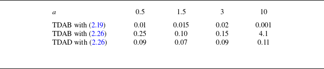
is equal to zero. For the TDAB, the location of the dividing surface is either prescribed by (2.26) or (2.19). The relative error between the TDA solutions and the ODA reference one has been assessed from the maximum velocity in the fluid region as
 $|(u^f_{{max}} - u_{{max}})/u_{{max}}|$
and is documented in table 2.
Comparison of ODA, using the permeability distribution (3.10) with
 $y_0=0$
and with
 $\tilde \alpha$
given by (3.13), and the TDA solutions for a constant thickness
 $\delta =0.01$
of the diffuse interface and different values of
 $a$
with
 $\unicode{x03B5} _H=0.8$
. The Darcy number is adjusted to
 $Da = \unicode{x03B5} _H (\delta /a)^2$
to maintain
 $\delta$
constant. The extension of the diffuse interface is indicated by a grey zone limited by dotted horizontal lines. The horizontal solid lines indicate the locations of the dividing surface. Here, ‘TDAB min’ and ’TDAB no-slip’ refer to TDAB solutions with a dividing surface prescribed by (2.19) and (2.26), respectively.

For all tested values of the parameter
 $a=\delta /\delta _B$
, an excellent agreement of the TDA and ODA solutions is observed outside the interfacial region. We note that the solutions to TDAB with
 $\tilde {y_i}$
prescribed by (2.19) are the most accurate ones yielding a remarkable agreement with the ODA solution outside the interfacial region. For the largest tested value
 $a=10$
, the TDAB solution with (2.26) presents a divergence in the Brinkman sub-layer as
 $u^p|_i$
rises to an unrealistic value. As a consequence, a noticeable discrepancy with the ODA reference is observed in that case. This underlines that the location of the dividing surface may not be freely chosen within TDAB at large values of
 $a$
.
At
 $a=0.5$
, the ODA solution presents significant deviations of the velocity profile in the porous medium from the Darcy seepage velocity, which demonstrates that the Brinkman sub-layer is not contained within the interfacial region in that case. Panel (a) compares the solution of the GTE equations (2.1) with the TDAB solutions. An excellent agreement is found outside the interfacial region and the Brinkman sub-layer provided
 ${\tilde y}_i$
is prescribed by (2.19). In particular, the maximum velocity of the flow is very accurately captured. Similar excellent agreements are observed at
 $a=1.5$
(panel b),
 $a=3$
(panel c) and
 $a=10$
(panel d). We note that, for
 $a \geqslant 3$
, the Brinkman diffusion sub-layer of the TDAB solution is already included within the interfacial region and that the largest deviations between ODA and TDAB are reported in the Brinkman sub-layer due to the exponential nature of the TDAB solution.
We next turn to the parallel flow conditions investigated by Hernandez-Rodriguez et al. (Reference Hernandez-Rodriguez, Angot, Goyeau and Ochoa-Tapia2022) and corresponding to figure 5, for which the ratio
 $a=\delta /\delta _B$
of the thicknesses of the interfacial region and Brinkmann sub-layer ranges from
 $15.81$
to
 $237.15$
(see figure 8). For these large values of
 $a$
, the Brinkman sub-layer of the TDAB solution is entirely contained within the interfacial region. Because of the exponential nature of the porous-side solution (2.10), it is not possible to locate the dividing interface for the TDAB at a position which differs from (2.19) by a distance that is larger than a few
 $\delta _B$
. As a consequence, the TDAB velocity is oriented along with the pressure gradient in the fluid layer in the vicinity of the dividing surface. The occurrence of this seemingly unrealistic backflow region is a consequence of the reduction of the extension of the porous medium in comparison with the ODA permeability distribution. The reduction of the drag exerted by the solid matrix on the fluid is compensated by a negative slip length at the dividing surface within the TDAB.


However, comparisons of the TDAB and ODA solutions show again a remarkable agreement outside of the interfacial region. In contrast, with the TDAD, the dividing interface can be freely chosen. Besides, at large values of
 $a$
, the coefficients
 $L$
,
 $F$
,
 $G$
and
 $M$
are nearly constant. We have tabulated those coefficients in table 3 as functions of the bulk porosity
 $\unicode{x03B5} _H$
for a dividing interface located at
 ${\tilde y}_i = 0$
. The values of these coefficients for a different location of the dividing surface can be computed easily using (2.25).
Values of the coefficients
 $L$
,
 $F$
,
 $G$
and
 $M$
as functions of the bulk porosity
 $\unicode{x03B5} _H$
for
 $a=10^3$
corresponding to the permeability distribution (3.10) with
 $y_0=0$
, a dividing interface located at
 ${\tilde y}_i = 0$
and
 $\tilde \alpha$
given by (3.13). These coefficients for a different choice of the dividing surface location can be obtained from (2.25).

For the value
 $L=0.0283$
corresponding to
 $\unicode{x03B5} _H=0.4$
, the solution to the TDAD is in close agreement with both the ODA and TDAB. Notice that the values of the coefficient
 $F$
in table 3 are all negative, which is counterintuitive, but can be easily understood by considering the permeability distribution (3.10). Indeed,
 $1/\kappa$
is severely skewed, as can be observed from figure 4. Thus, locating the dividing surface at the middle of the interfacial region results in an overestimation of the drag exerted onto the flow within the TDA in comparison with the ODA. This effect is compensated by a negative value of the resistance coefficient
 $F$
.


3.5. Comparison with experimental results
We end this section with a comparison with the experimental results obtained by Goharzadeh et al. (Reference Goharzadeh, Khalili and Jørgensen2005). These authors studied the velocity profile at the transition region of a flow overlying a packed bed of monodisperse spherical glass beads in a rectangular channel. We have solved the Darcy–Brinkman and Darcy equations (2.3) and (2.4) taking into account the width of the channel. A weighted-residual Galerkin method was employed with Legendre polynomials to represent the dependency of the solution with respect to the transverse direction. Taking into account the symmetry of the solution with respect to the vertical half-plane, a total of seven polynomials, corresponding to a degree up to twelve, was found to be sufficient. The limits of the interfacial region were identified by Goharzadeh et al. (Reference Goharzadeh, Khalili and Jørgensen2005) from the experimental records to extend from the uppermost ordinate of the beads to a depth roughly equal to the bead diameter. We have adjusted the extension
 $y=\pm \delta$
of the diffuse interface to coincide with the region of variation of porosity reported in the experiment. The parameters
 $\tilde \alpha$
and
 $y_0$
of the ad hoc permeability distribution (3.10) are adjusted using (3.13) and
 $y_0=0$
. We compare in figure 9 the experimental and numerical velocity profiles at the vertical symmetry plane of the channel for the experiment with glass beads of diameter 6.5 mm (labelled GB3 by Goharzadeh et al.). To facilitate the comparison with figure 5 in Goharzadeh et al. (Reference Goharzadeh, Khalili and Jørgensen2005), the vertical coordinate
 $\bar y$
is provided in dimensional units with an origin
 ${\bar y} =0$
matching Goharzadeh et al.’s choice, i.e. the upper limit of the region of variation of the porosity. Parameters are
 $\unicode{x03B5} _H=0.41$
,
 $Da=2.03\times 10^{-6}$
and
 $a=18.3$
. Since the pressure gradient applied in the experiment is unknown, we have adjusted it in our numerical simulations by requiring that the maximum velocity of the ODA solution matches the experimental one. The TDAD and TDAB solutions have been computed with the same pressure gradient as with the ODA computation. The deviations of the computed solutions with respect to the experimental results are evaluated using the norm
 $\| u\|_2= \sqrt {N^{-1}\sum _{j=1}^N ( u(y=y_j) )^2}$
, where
 $y_j$
refer to the locations at which experimental data are provided in the fluid layer outside the interfacial region (
 $y_j\gt \delta$
). Table 4 compares the relative errors
 $\| u^f - u^{{exp}}\|_2/\| u^{{exp}}\|_2$
and
 $\| u^f - u\|_2/\| u\|_2$
with respect to the experimental data and the ODA solution.
Relative error in per cent of the numerical solutions with respect to the experimental data by Goharzadeh et al. (Reference Goharzadeh, Khalili and Jørgensen2005) and with respect to the ODA solution corresponding to figure 9. The relative error is computed as
 $\| u^f - u^{{exp}}\|_2/\| u^{{exp}}\|_2$
and
 $\| u^f - u\|_2/\| u\|_2$
for the experimental data locations
 $y_j$
in the fluid layer (
 $y_j \gt \delta$
).

Comparison of velocity profiles with the experimental results by Goharzadeh et al. (Reference Goharzadeh, Khalili and Jørgensen2005). Here,
 $\unicode{x03B5} _H=0.41$
,
 $\kappa _H= 1.3\times 10^{-8}$
 $\textrm {m}^2$
,
 ${\bar \delta }=3.25$
mm. The ODA solution is again computed using (3.10), with
 $\tilde \alpha$
given by (3.13). The extension of the diffuse interface region is indicated by horizontal dotted lines. The locations (2.19) and (2.26) of the dividing surface are indicated by thin horizontal red and green lines, respectively.

Note the close agreement of the ODA solution with the experimental records, except somehow in the interfacial region. This relative disagreement can be explained partly by the difference in the definition of the averaged velocity in the volume-averaging theory and in the experimental work of Goharzadeh et al. (Reference Goharzadeh, Khalili and Jørgensen2005). Goharzadeh et al. proceeded to an averaging of their measurements by particle image velocimetry over ten different sections of the channel, which is a significantly different process than averaging locally the PSS solution over a representative volume of radius
 $r_0\approx \delta$
.
Interestingly, the TDAD solution is closer to the ODA reference one than the TDAB solution is, which suggests that accounting for the Brinkman diffusion effects does not necessarily improve the TDA predictions of the flow field whenever
 $a$
is large. Besides, TDAB predicts either an unrealistically large porous-side interfacial velocity
 $u^p|_i$
, when the dividing interface is located at
 ${\tilde y}_i$
given by (2.26), or predicts a backflow region, where the velocity is oriented as that of the direction of the pressure gradient, if
 ${\tilde y}_i$
is given by (2.19). The observed limitations of the Brinkman approach for a channel flow result from the exponential variation of velocity within the Brinkman sub-layer whenever its extension
 $\delta _B$
is much smaller than the extension of the interfacial region
 $\delta$
. We note that Valdés-Parada et al. (Reference Valdés-Parada, Aguilar-Madera, Ochoa-Tapia and Goyeau2013) did not account for this rapid variation, as they assumed slow-varying velocity profiles in the interfacial region. They thus neglected the Brinkman sub-layer, which amounts to neglecting the Brinkman corrections.
4. Validation: stagnation point flow
In this section, we consider an example of non-parallel 2-D flow. We extend the well-known solution of a viscous stagnation point flow on a solid wall (Schlichting & Gersten Reference Schlichting and Gersten2001) to the case of a porous one with suction. The porous medium extends from
 $y=-h$
to the fluid–porous boundary at
 $y=0$
, whereas the overlying fluid layer extends to
 $y={ H-h}$
with
 $H \gg \delta$
in order to mimic a plane irrotational flow impinging a wall. The flow is assumed to be potential far from the boundary, i.e.
 $u\approx x$
,
 $v\approx - y + cst.$
,
 $p \approx -({x^2+ y^2})/{2} + cst.$
. We introduce a suction velocity
 $v_s = -\tilde {A}\, Da$
at the bottom
 $y=-h$
of the porous medium. In this test case, the Darcy seepage velocity is oriented non-trivially with respect to the direction of the porous–fluid interface. Besides,
 $v_y \ne 0$
in the interfacial region will enable us to check the presence of a pressure jump and a normal velocity. The length scale is adjusted to set the Reynolds number to unity without loss of generality. All presented computations have been performed with the ad hoc permeability distribution (3.10). However, we checked that the use of the permeability distribution (3.1) yields similar conclusions in terms of the accuracy of TDA with respect to the ODA reference and the corresponding results are not shown.
Following Schlichting & Gersten (Reference Schlichting and Gersten2001), we introduce the ansatz
 \begin{align} u = xf'(y), \qquad v= - f(y), \qquad p = - \frac {x^2}{2} - g(y), \end{align}
which enables us to reduce the resolution of the original 2-D problem to a 1-D one. Within the ODA, the system of equations to be solved thus reads
 \begin{align} \frac {f'''}{\unicode{x03B5} } - \frac {f'}{\kappa } & = \frac {1}{\unicode{x03B5} } \left [ \frac {(f')^2 - \textit{ff}\,''}{\unicode{x03B5} } + \frac {\unicode{x03B5} '}{\unicode{x03B5} ^2}{f\!\!f}' \right ] - 1 , \\[-12pt] \nonumber \end{align}
 \begin{align} \frac {f''}{\unicode{x03B5} } - \frac {f}{\kappa } & = \frac {1}{\unicode{x03B5} } \left [ -\frac {\textit{ff}\,'}{\unicode{x03B5} } + \frac {\unicode{x03B5} '}{\unicode{x03B5} ^2}f^2 \right ] + g' , \\[12pt] \nonumber \end{align}
with the associated boundary conditions
 \begin{align} f(-h)= \tilde {A}\,Da, \quad f'(-h)=g(-h)=0,\quad f'({ H-h}) = 1 . \end{align}
Within the TDA, the Darcy–Brinkman equations (2.3) yield
 \begin{align} \frac {{f^p}'''}{\unicode{x03B5} _H} - \frac {{f^p}'}{Da} & = \frac {({f^p}')^2 - f^p {f^p}''}{\unicode{x03B5} _H^2} - 1,\quad \frac {{f^p}''}{\unicode{x03B5} _H} - \frac {f^p}{Da} = -\frac {f^p\,{f^p}'}{\unicode{x03B5} _H^2} + {g^p}' , \\[-12pt] \nonumber \end{align}
 \begin{align} {{f}^f}''' & = ({{f}^f}')^2 - {f}^f {{f}^f}'' - 1 , \quad {{f}^f}'' = - {f}^f\,{{f}^f}' + {g^f}' , \\[12pt] \nonumber \end{align}
which set is closed by (4.3). Considering instead a Darcy flow within the porous medium (TDAD), this system of equations reduces to (4.4b
) with
 $f^p =Da (\tilde {A}+y+h)$
and
 $g^p= - [\tilde {A}(y+h) + ({1}/{2})(y+h)^2 ]$
.
4.1. First test
Streamlines in the porous region and in the vicinity of the diffuse interface for the flow around a stagnation point with suction. Here,
 $H=10$
,
 $h=0.5$
,
 $Da = 10^{-3}$
,
 $\unicode{x03B5} _H=0.8$
(
 $a=1.68$
),
 $\tilde {A}=2$
. The ODA solution to (4.2) is indicated with dashed lines. Panels b and c differ only by the choice of location of the dividing surface.

We first consider the case of a relatively large porosity
 $\unicode{x03B5} _H=0.8$
, typical of metal foams, and a large permeability with a Darcy number
 $Da = 10^{-3}$
, in order to generate a significant flow in the porous region. The height
 $H=10$
of the numerical domain is chosen large enough in order to recover a potential flow far from the porous wall. The extension of the interfacial region is chosen to be of the order of the pore size estimated by the Carman–Kozeny relation (3.12), i.e.
 $2\delta =\ell$
, which gives
 $a={\tilde \alpha } = 1.89$
. Figure 10 illustrates the flow pattern and its symmetry around the stagnation point located at
 $x=0$
, in the porous region and at the diffuse interface. The streamlines are obtained from the expression
 $x\,f(y)$
of the streamfunction corresponding to the ODA solution, to the TDAB solution to the Darcy–Brinkman equation (4.4) with the jump boundary conditions (2.15) and to the TDA solution to the Darcy equation (2.4) with the boundary conditions (2.23). An excellent agreement of the TDAD and TDAB solutions to the reference ODA solution is observed in the fluid and porous regions outside the diffuse interface. The TDAB solution is the closest to the reference ODA solution either if the dividing surface location is fixed by (2.26) or (2.19) (panels b and c). With the choice (2.19), the TDAB solution presents a sink of mass at the crossing of the dividing surface and the vertical axis (panel c of figure 10). Although the presence of this sink seems unrealistic, it is required to adjust the amount of mass penetrating the porous medium whose resistance to the flow is underestimated with respect to the ODA for that choice of the dividing surface location.
Figure 11 further offers a direct comparison of the ODA solution with TDAB solutions to the Darcy–Brinkman equation (4.4) with the jump boundary conditions (2.15), as well as the TDAD solution to (4.4b
) with the Darcy flow
 $f^p =Da (\tilde {A}+y+h)$
and
 $g^p = - (\tilde {A}(y+h) + ({1}/{2})(y+h)^2 )$
and the DTR model (2.24). The dividing surface is prescribed at the same location for both TDAB and TDAD by (2.26).
Comparison of ODA solution to (4.2), labelled ‘ODA’, with the TDA solutions, using the permeability distribution (3.10) with
 $y_0=0$
with
 $\tilde \alpha$
given by (3.13) (
 $\unicode{x03B5} _H=0.8$
,
 $H=10$
,
 $h=0.5$
,
 $\delta =0.01$
,
 $a=1$
and
 $\tilde {A}=2$
). The location,
 ${\tilde y}_i =- 4\times 10^{-5}$
of the dividing surface is prescribed by (2.26) and indicated by a solid horizontal line.

The relative error of the TDA solutions with respect to the ODA reference is computed at the upper limit of the interfacial region, i.e.
 $|(z^f|_{y=\delta } - z|_\delta )/z|_\delta |$
, where
 $z=f$
,
 $f'$
,
 $f''$
and
 $g$
are documented in table 5. For TDAD, the error estimates are corrected by taking into account the deviations induced by the presence of a Brinkman layer at the lower wall
 $y=-h$
which is not captured by the Darcy model. The TDAB predicts the velocity field (
 $u \propto f'$
and
 $v \propto f$
) and pressure field (
 $p\propto g$
) very accurately. We note, however, that the TDAB overestimates somehow the velocity outside the diffuse interface in the porous region, as the Brinkman sub-layer is not contained within the interfacial region at
 $a=1$
. The solution to the TDAD, assuming a Darcy flow in the porous medium and using the DTR transfer model, is also very precise, even though it does not capture the two Brinkman sub-layers at the bottom and at the top predicts a pressure field which differs slightly from the ODA solution. Noteworthy is that the discrepancy between the pressure fields arises only from neglecting the bottom Brinkman sub-layer as TDAB and TDAD predict similar pressure jumps at the dividing surface.
Relative error in per cent of the TDA solutions with respect to the ODA reference computed at the upper limit of the interfacial region for the computations displayed in figures 11 and 12. The relative error is computed at the upper limit of the interfacial region
 $y=\delta$
. Concerning TDAD, the error estimates takes into account the deviations induced by the Brinkman layer at the lower wall.

Figure 12 compares again the solutions of the ODA, TDAD and TDAB for the stagnation point problem but for a thinner Brinkman sub-layer (
 $a=20$
) and
 $\unicode{x03B5} _H=0.4$
. This time, the dividing surfaces for the TDAD and TDAB are placed at different locations, corresponding to a no-slip boundary condition for the tangential velocity, i.e. (2.26), and a minimum of the jump of tangential velocities, i.e. (2.19), respectively. The relative error of the TDA solutions, computed as in the former case, is documented in table 5. Both TDAD and TDAB are again very accurate, precisely capturing the velocity and pressure fields in the bulk of the porous and fluid regions. In particular, the prediction of the pressure by TDAD matches this time the ODA solution with great fidelity. Note that, depending on the location of the dividing surface, the pressure jump changes sign as a consequence of overestimating or underestimating the resistance of the porous medium to the flow. Besides, contrary to the TDAB solution, the TDAD solution does not present an unrealistic negative normal velocity. This again suggests that, whenever the Brinkman sub-layer is included within the interfacial region (
 $a\gg 1$
), the TDAB should be discarded in favour to TDAD.
Comparison of ODA solution with the TDA solutions (
 $\unicode{x03B5} _H=0.4$
,
 $H=10$
,
 $h=0.5$
,
 $\delta =0.01$
,
 $a=20$
,
 ${\tilde A}=2$
and
 $y_0=0$
). Same as in figure 11 except for the locations of the dividing surface. The horizontal black and violet lines refer to (2.26) and (2.19), respectively.

Comparison of ODA solution, labelled ‘ODA’, with the TDAD and TDAB solutions, with the TDAD solution with Naqvi & Bottaro’s boundary conditions (4.5) and with the PSS solution computed by Naqvi & Bottaro (Reference Naqvi and Bottaro2021) (
 $H=30$
,
 $h=4.75$
,
 $\unicode{x03B5} _H=0.9999$
,
 $\delta =\ell /2$
with
 $\ell =0.5$
,
 $a=1.346$
,
 $A=0$
,
 ${\tilde \alpha } = \ell /(2\delta _B)$
and
 $y_0=0$
). The extension of the interfacial region is indicated by two horizontal lines at
 $y=\pm \delta$
. The dividing surface is located at
 $y=0$
except for the Naqvi & Bottaro TDAD solution (
 $y=0.25$
).

4.2. Second test
To conclude this section, we consider a test case proposed by Naqvi & Bottaro (Reference Naqvi and Bottaro2021). These authors considered an impinging jet on a porous wall with a very high porosity,
 $\unicode{x03B5} _H=0.9999$
, and an impermeable bottom wall (
 $\tilde {A}=0$
). The porous medium is made of a regular arrangement of ten rows of cylinders with an inter-grain distance equal to
 $\ell =0.5$
. The Darcy number is estimated from the streamwise velocity profiles obtained by Naqvi & Bottaro to be
 $Da =0.0345$
. The extension of the interfacial region is chosen to match the inter-grain distance, thus
 $\delta =0.25$
and
 $a=1.346$
. The permeability distribution (3.10) is again invoked with (3.11), i.e.
 ${\tilde \alpha } = \ell /(2\delta _B)$
as the Carman–Kozeny relation is not reliable for such a high value of the porosity. The transition region is centred on the envelope of the first row of cylinders, which shifts the
 $y$
coordinate by a distance
 $\ell /2$
with respect to Naqvi & Bottaro’s definition of the test case. Thus,
 $h=4.75$
,
 $H=30$
and
 $y_0=0$
. The limit of the uppermost cell, corresponding to the location of the TDA dividing surface by Naqvi & Bottaro is thus
 $y=\delta =0.25$
. Figure 13 compares the velocity distribution of the ODA and TDA solutions with the PSS performed by Naqvi & Bottaro. Associated relative errors are reported in table 6. The reasonable agreement we obtain suggests that the ad hoc permeability distribution (3.10) enables us to reproduce satisfactorily the PSS provided that the parameter
 $y_0$
corresponds to the limit of the solid matrix of the porous material. However, although our computations match reasonably well the PSS for the tangential velocity, some significant differences can be observed for the normal component. The solution to the TDAB is again in excellent agreement with the ODA solution. However, as the Brinkman sub-layer is not fully included into the interfacial region, the velocity distribution predicted by the TDAD is less accurate than with the TDAB. In particular, the normal velocity component predicted by TDAD departs from the ODA reference, whereas the TDAB solution is in good agreement with ODA. This discrepancy emanates from the high value of the Darcy number promoting a significant tangential velocity
 $u^p$
in the porous medium, which is neglected in the derivation of the boundary conditions (2.23) but accounted for in the derivation of (2.15). Similarly, the pressure field predicted by TDAD is somewhat off the mark, as the drag exerted by the Brinkman boundary layer at the bottom impermeable wall is not accounted for by the Darcy equation. Yet, the jump of pressure at the dividing surface predicted by TDAD is in close agreement with the one predicted by TDAB.
Relative error with respect to the PSS solution and to the ODA solution for the simulations presented in figure 13. The relative error is computed with the norm
 $\| x\|_2= \sqrt {N^{-1}\sum _{j=1}^N (x(y=y_j))^2}$
, where
 $y_j$
correspond to the locations of the PSS data in the fluid region above the interfacial transition layer.

The boundary conditions derived by Naqvi & Bottaro (Reference Naqvi and Bottaro2021)
 \begin{align} u^f|_i = \lambda \left (u_y^f \big|_i + v_x^f \big|_i \right ) - \kappa ^{itf} p_x^{{ p}} \big|_i,\quad v^f \big|_i = v^p \big|_i,\quad p^f \big|_i - 2 v_y^f \big|_i = p^p \big|_i,\, \end{align}
are applied at the uppermost limit of the periodic cells constituting the porous medium, i.e. at
 $y=\ell /2=0.25$
. The coefficients
 $\lambda$
and
 $\kappa ^{itf}$
have been tabulated by Naqvi & Bottaro, which read for the present case (2-D regular arrangement of cylinders) as
 $\lambda = 0.6188\,\ell$
and
 $\kappa ^{itf}=0.2585\,\ell ^2$
. Comparisons of the TDAD solutions with the STR model (2.23) and with Naqvi & Bottaro’s boundary conditions (4.5) show that both models yield close results except for the normal component of the velocity.
Finally, we present in figure 14 a comparison of the streamlines and pressure field computed with the ODA, TDAD and TDAB. The reader is invited to compare with figure 10 in Naqvi & Bottaro (Reference Naqvi and Bottaro2021). The flow pattern and pressure field predicted either by TDAB or TDAD reproduce satisfactorily the ODA solution.
Streamlines (left) and pressure field (right) predicted by the ODA (top row) and the TDA (middle and lower rows). Same as in figure 13.

5. Concluding remarks
The present investigation has considered a long-standing challenge to accurately describe and model the transport phenomena in a fluid–porous medium system and the transitional region between the two domains responsible for interfacial mass and momentum transfer. Our starting point is the GTE equations (2.1) as a valid macroscopic description of the momentum transfer at the fluid–porous interface (Hernandez-Rodriguez et al. Reference Hernandez-Rodriguez, Angot, Goyeau and Ochoa-Tapia2022). Following Valdés-Parada et al. (Reference Valdés-Parada, Aguilar-Madera, Ochoa-Tapia and Goyeau2013), we have formulated a MCP which we solve numerically to yield the appropriate boundary conditions (2.15) and (2.23) associated with the Darcy–Brinkman equations and the Darcy equations, respectively. Our work extends the pioneering work of Valdés-Parada et al. (Reference Valdés-Parada, Aguilar-Madera, Ochoa-Tapia and Goyeau2013) to non-parallel flows. In particular, in contrast to Valdes-Parada et al., instead of assuming a constant TDA velocity field in the interfacial region, we take into account its asymptotic solution. This point is crucial as the porous-side TDAB velocity presents an exponential behaviour in the Brinkman sub-layer, defined as the region where Brinkman diffusion terms are effective. Moreover, our formulation enables us to freely locate the dividing interface, provided that the MCP is well posed, which may be not guaranteed in the limit of a thin Brinkman sub-layer (
 $a\gg 1$
) when the Brinkman corrections are taken into account. We have identified two relevant different locations for the dividing surface which enable us to minimise the divergence of the TDA solution to the ODA reference for parallel flows depending on whether Brinkman corrections are accounted for or not. In contrast to Angot et al. (Reference Angot, Goyeau and Ochoa-Tapia2017), our formulation takes into account the details of the permeability distribution within the interfacial region through the numerical resolution of the MCP.
Validation of our new formulation has been carried out for a parallel flow in a channel bounded by a porous medium, and for the non-parallel boundary layer at the impact of a potential flow impinging a porous wall in presence of suction. With this aim, we have proposed an ad hoc expression for the permeability distribution, which preserves the invariance of the ODA velocity in the fluid region as the radius
 $r_0$
of the averaging volume is varied (Valdés-Parada & Lasseux Reference Valdés-Parada and Lasseux2021). The ad hoc permeability distribution (3.10) is a valid substitute for numerically obtained ones whenever PSS are too costly or unavailable as for most experimental data. We note that we have not been able to find continuous explicit permeability distributions which satisfy this invariance. In particular, the permeability distribution proposed by Valdés-Parada et al. (Reference Valdés-Parada, Aguilar-Madera, Ochoa-Tapia and Goyeau2013) does not verify this property. The derived boundary conditions (2.15) and (2.23) enable TDAD and TDAB to closely recover the ODA reference solution for the two tested permeability distributions.
For parallel flows, the solutions to our ODA formulation with the proposed ad hoc permeability distribution satisfactorily compare with the averaged PSS solutions when the thickness of the interfacial region,
 $\delta$
, is adjusted to the size
 $r_0$
of the averaging volume. We thus conclude that our ODA formulation with
 $\delta =r_0$
is a valid reference. The jump boundary conditions (2.15) and (2.23), for the TDAB and TDAD, respectively, enable us to recover precisely the ODA solutions for the channel and impinging flow test cases. In particular, comparisons with the experiments and with the PSS present a good agreement, with a relative error limited to a few per cent, as illustrated in tables 4 and 6. These comparisons have been conducted by adjusting two parameters
 $y_0$
, appearing in the ad hoc permeability distribution (3.10), and the interface thickness
 $\delta$
. We recall that parameter
 $\tilde \alpha$
is set to
 $\ell /(2 \delta _B)$
, where
 $\ell$
is the pore scale and the Brinkman thickness
 $\delta _B$
depends only on the bulk properties of the porous material. Parameter
 $y_0$
has been set to the mean location of the solid matrix of the porous region, whereas
 $\delta$
has been adjusted to match either the extension of the porosity variation reported in the experiments (Goharzadeh et al. Reference Goharzadeh, Khalili and Jørgensen2005), the averaging radius
 $r_0$
of the averaged PSS (Valdés-Parada & Lasseux Reference Valdés-Parada and Lasseux2021; Hernandez-Rodriguez et al. Reference Hernandez-Rodriguez, Angot, Goyeau and Ochoa-Tapia2022) or half of the inter-grain distance
 $\delta =\ell /2$
(Naqvi & Bottaro Reference Naqvi and Bottaro2021). Our main objective has been to propose boundary conditions for the TDA which enable us to reproduce very accurately the ODA results. This has been achieved for all tested permeability and porosity distributions for parallel and non-parallel flows. Besides, comparisons with averaged PSS and experiments have been based on proposed ad hoc permeability and porosity distributions, yielding a convincing qualitative agreement. To achieve an accurate agreement with experiments and PSS demands that we have access to information at the pore scale and therefore to the permeability and porosity profiles accounting for that information. Strategies to obtain this information have already been proposed elsewhere by e.g. Valdés-Parada & Lasseux (Reference Valdés-Parada and Lasseux2021) and Hernandez-Rodriguez et al. (Reference Hernandez-Rodriguez, Angot, Goyeau and Ochoa-Tapia2022).
The extension of the interfacial region
 $\delta$
corresponds closely to the radius
 $r_0$
of the averaging volume, which is chosen by the user. Therefore
 $a=\delta /\delta _B$
is a parameter chosen by the user and corresponds to the minimal scale,
 $r_0\sim \delta$
, which is represented by the macroscopic model derived from the volume-averaging technique. In our comparisons with the filtered PSS, it is clear that
 $\delta$
must coincide with
 $r_0$
to yield quantitative comparisons between ODA, TDA and PSS. With respect to the experiments, our comparisons suggest that
 $\delta$
should correspond to the minimal scale at which a macroscopic approach is meaningful, which corresponds to
 $2\delta =\ell$
, where
 $\ell$
is the characteristic pore scale.
Our results suggest that the TDAB may be avoided whenever the Brinkman penetration depth is small compared with the size of the averaging volume, i.e.
 $\delta =r_0 \gg \delta _B$
or
 $a=\delta /\delta _B \gg 1$
. In that limit, the Brinkman sub-layer is entirely contained within the interfacial region and Brinkman diffusive corrections are effective on a scale that is smaller than the lowest resolved scale
 $r_0$
. The TDAD solutions approach the ODA reference as accurately as TDAB solutions in that limit and are much easier to compute. However, TDAB is more accurate for
 $\delta \sim \delta _B$
, i.e.
 $a=0(1)$
, and should be preferred in that case.
Coefficients of the STR model (2.23) of momentum and mass transfer within TDAD have been tabulated in table 3 as functions of the porosity
 $\unicode{x03B5} _H$
in the limit
 $a\gg 1$
, which enables an easy implementation.
The proposed models for the mass and momentum transports at a fluid–porous interface present a pathway for extending the study to multiphase flows involving fluid–porous domains and multi-scale flow problems. Further, an extension of the study to include anisotropy of the porous medium is sketched in Appendix C. Inclusion of higher-dimensional flow, inhomogeneous porous layers and inertial effects is feasible and may require a higher-order description in terms of the interfacial thickness
 $\delta$
. The investigations on these and other relevant applications are in progress.
Funding
S.M. thanks to Anusandhan National Research Foundation (ANRF), Government of India for providing research grant through ANRF-TARE (TAR/2023/000076) for carrying out this research work. C.R.Q. thanks B. Goyeau for fruitful discussions and for providing insights on the subject. C.R.Q. acknowledges support from project FILLMORE, grant ANR-23-CE51-0046-03 of the French National Research Agency (ANR).
Declaration of interests
The authors report no conflict of interest.
Appendix A. Macroscopic closure problem
The MPC verified by the macroscopic deviation velocities
 ${\hat u}^{f,p} = u - u^{f,p}$
,
 ${\hat v}^{f,p} = v - v^{f,p}$
and pressure
 ${\hat p}^{f,p} = p - p^{f,p}$
is obtained after substitution in (2.7) using the expressions (2.10). It reads
 \begin{align} {\hat u}^f_{x} + {\hat v}^f_{y} & = 0 , \\[-12pt] \nonumber \end{align}
 \begin{align} {\hat u}^f_{yy} - \frac {\unicode{x03B5} }{\kappa } {\hat u}^f & = \frac {\unicode{x03B5} }{\kappa } u^f \big|_i + \frac {\unicode{x03B5} }{\kappa } (y-y_i) u_y^f \big|_i , \\[-12pt] \nonumber \end{align}
 \begin{align} {\hat v}^f_{yy} - \frac {\unicode{x03B5} }{\kappa } {\hat v}^f - \unicode{x03B5} {\hat p}^f_y & = \frac {\unicode{x03B5} }{\kappa } v^f \big|_i + \frac {\unicode{x03B5} }{\kappa } (y - y_i) v_y^f \big|_i + \left [ \frac {\unicode{x03B5} }{2\kappa } (y - y_i)^2 + \unicode{x03B5} -1 \right ] v^f_{yy} \big|_i, \\[12pt] \nonumber \end{align}
in the fluid region and
 \begin{align} {\hat u}^p_{x} + {\hat v}^p_{y} & = 0, \\[-12pt] \nonumber \end{align}
 \begin{align} {\hat u}^p_{yy} - \frac {\unicode{x03B5} }{\kappa } {\hat u}^p & = \left (\frac {\unicode{x03B5} }{\kappa } -\frac {1}{\delta _B^2}\right ) \left [ C\, u^p \big|_i + S\, \delta _B u_y^p \big|_i \right ] , \\[-12pt] \nonumber \end{align}
 \begin{align} {\hat v}^p_{yy} - \frac {\unicode{x03B5} }{\kappa } {\hat v}^p - \unicode{x03B5} {\hat p}^p_y & = \left ( \frac {\unicode{x03B5} }{\kappa } - \frac {\unicode{x03B5} }{Da} \right )v^p \big|_i + \left (\frac {\unicode{x03B5} }{\kappa } - \frac {1}{\delta _B^2} \right ) \delta _B S\, v_y^p \big|_i \nonumber \\ & \quad + \left [ \left (\frac {\unicode{x03B5} }{\kappa } - \frac {1}{\delta _B^2} \right ) \delta _B^2 C + \frac {\unicode{x03B5} }{\unicode{x03B5} _H} \left (1 - \frac {Da}{\kappa } \right ) \right ] v^p_{yy} \big|_i , \\[12pt] \nonumber \end{align}
in the porous region, where
 $C(y) = \cosh ( ({y-y_i}/{\delta _B}) )$
and
 $S(y) = \sinh (({y-y_i}/{\delta _B}) )$
.
The MCP (A1) is completed by the boundary conditions at the dividing interface
 \begin{align} {\hat u}^f \big|_i + u^f \big|_i & = {\hat u}^p \big|_i + u^p \big|_i,\quad {\hat u}^f_y \big|_i + u^f_y \big|_i = {\hat u}^p_y \big|_i + u^p_y \big|_i , \\[-12pt] \nonumber \end{align}
 \begin{align} {\hat v}^f \big|_i + v^f \big|_i & = {\hat v}^p \big|_i + v^p \big|_i,\quad {\hat p}^f \big|_i + p^f \big|_i = {\hat p}^p \big|_i + p^p \big|_i , \\[12pt] \nonumber \end{align}
which express the continuity of the ODA solution at the fictitious dividing interface, and the requirement that the ODA and TDA solutions match outside the interfacial region so that
 \begin{align} \lim _{y\to \pm \infty } {\hat u} = \lim _{y\to \pm \infty } {\hat v } = \lim _{y\to \pm \infty } {\hat p}= 0 . \end{align}
Following Valdés-Parada et al. (Reference Valdés-Parada, Aguilar-Madera, Ochoa-Tapia and Goyeau2013), the linearity of the system (A1), (A2) and (A3) enables to make use of the superposition theorem and to look for its solution in the form of (2.11). The continuity equation yields directly
 $g_1'=g_2'=0$
and
 $g'_3=f_1$
,
 $g_4'=f_2$
,
 $g_5'=f_3$
,
 $g_6'=f_4$
. From the momentum balances,
 $f_j$
,
 $g_j$
and
 $m_j$
also verify
 ${m_7}_y=0$
and
 \begin{align} \left (f_j^f\right )_{yy} - \frac {\unicode{x03B5} }{\kappa } f^f_j & = {\Pi }^f_{fj}, \qquad \left (f_j^p\right )_{yy} - \frac {\unicode{x03B5} }{\kappa } f^p_j = {\Pi }^p_{fj} , \\[-12pt] \nonumber \end{align}
 \begin{align} \left (m^f_j\right )_{y} -\frac {1}{\unicode{x03B5} } \left (g^f_j\right )_{yy} + \frac {1}{\kappa } g^f_j & = {\Pi }^f_{gj},\qquad \left (m^p_j\right )_{y} -\frac {1}{\unicode{x03B5} } \left (g^p_j\right )_{yy} + \frac {1}{\kappa } g^p_j = {\Pi }^p_{gj} , \\[12pt] \nonumber \end{align}
where the expressions of the source terms
 $\Pi$
are defined in table 7. System (A4) is completed by the boundary conditions
 \begin{align} f^f_j\big|_i - f^p_j \big|_i & = \delta _{j1} - \delta _{j2},\qquad \left (f^f_j\right )_y \big|_i - \left (f^p_j\right )_y \big|_i = \delta _{j3} - \delta _{j4} , \\[-12pt] \nonumber \end{align}
 \begin{align} g^f_j \big|_i - g^p_j \big|_i & = \delta _{j1} - \delta _{j2},,\qquad m^f_j \big|_i - m^p_j \big|_i = \delta _{j7} , \\[12pt] \nonumber \end{align}
where
 $\delta _{jk}$
refers to the Kronecker symbol, i.e.
 $\delta _{jk}=1$
if
 $j=k$
and zero otherwise.
Expressions of the source terms in system (A4).

Some of the above functions
 $f_j$
,
 $g_j$
and
 $m_j$
can easily be determined analytically by considering some trivial flow solutions. For instance,
 $f_2^f=-1$
and
 $f_2^p=0$
. This trivial solution reflects the fact that a flow at rest can be decomposed into a tangential uniform flow in the fluid region and an opposite deviation, i.e.
 $u = u^f|_i + u^f|_i f_2^f$
, which thus gives
 $f_2^f=-1$
. Similarly, a constant pressure field can always be written as a discontinuity of pressure at the dividing interface plus an opposite deviation. Therefore,
 $m_7^f=0$
and
 $m_7^p=-1$
. Moreover, by considering the case of a uniform flow in the direction normal to the interface, in which case the ODA and TDA solutions should correspond to equal and constant normal velocities, i.e.
 $v^f=v^p$
and
 ${\hat v}^f= {\hat v}^p=0$
, it is easy to show that
 \begin{align} g_1^f & = 1,\quad g_1^p=0,\quad m_1^f = \int _y^{\infty } \frac {1}{\kappa } {\rm d}y,\quad m_1^p= \frac {y -y_i}{Da} +\int _y^{\infty } \frac {1}{\kappa } {\rm d}y , \\[-12pt] \nonumber \end{align}
 \begin{align} g_2^f & = -1,\quad g_2^p=0,\quad m_2^f=m_2^p=0 . \\[12pt] \nonumber \end{align}
Finally, integration of the continuity equation gives
 \begin{align} g_{i+2} = \int _{-\infty }^y f_i\,{\rm d}y\quad \hbox{for}\quad 1\leqslant i \leqslant 4. \end{align}
We solve equations (A4) with boundary conditions (A5) numerically by continuation using the software AUTO07p (Doedel et al. Reference Doedel, Champneys, Fairgrieve, Kuznetsov, Sandstede and Wang2008) in a domain of finite extension
 $ -{ l} \lt y \lt { l}$
, with
 $l \gg \delta$
. AUTO07p features an automatic mesh refinement method which is required to capture the sharp variations of the solutions within the Brinkman sub-layer. The following boundary conditions are applied:
 \begin{align} f^p_j \big|_{y=-l} = 0,\quad \left ( f^f_j\right )_y \big|_{y=l} = 0,\quad m^f_j \big|_{y=l} = 0. \end{align}
A.1. Macroscopic closure problem for Darcy flow
In this section, we formulate the MCP associated with the TDA where the flow in the homogeneous porous region is governed by the Darcy law. In that case, the deviation velocities and pressure verify in the porous region
 \begin{align} {\hat u}^p_{x} + {\hat v}^p_{y} & = 0, \end{align}
 \begin{align} {\hat u}^p_{yy} - \frac {\unicode{x03B5} }{\kappa } {\hat u}^p & = 0 , \end{align}
 \begin{align} {\hat v}^p_{yy} - \frac {\unicode{x03B5} }{\kappa } {\hat v}^p - \unicode{x03B5} {\hat p}^p_y & = \unicode{x03B5} {\hat p}^p_y \left ( \frac {\unicode{x03B5} }{\kappa } - \frac {\unicode{x03B5} }{Da} \right )v^p \big|_i. \end{align}
Using again the superposition theorem, the solution to the MCP is written as the summation (2.21) where the functions
 $f_2$
,
 $f_4$
,
 $g_1$
,
 $g_2$
,
 $g_4$
,
 $g_6$
,
 $m_1$
,
 $m_2$
,
 $m_4$
,
 $m_6$
and
 $m_7$
are solution to (A4), (A5) and (A7).
Appendix B. Expressions of the coefficients of the boundary conditions (2.15)
With the choice of a dividing surface location
 ${\tilde y}_i$
which differs from the location
 $y_i=\delta _B(-a+\ln a)$
at which the MCP is solved, the coefficients of the jump boundary conditions (2.15) are computed from the solution (2.10) of the asymptotic interfacial problem, which gives the expressions of the new coefficients as functions of the previous coefficients
 \begin{align} {\tilde a}_1 & = {\tilde C} \,a_1 - a {\tilde S} \,a_3,\quad {\tilde a}_2 = a_2 + \gamma ,\quad {\tilde a}_3 = {\tilde C}\,a_3 - \frac {\tilde S}{a} a_1 , \\[-12pt] \nonumber \end{align}
 \begin{align} {\tilde b}_1 & = {\tilde C} b_1 - {\tilde S} b_3,\quad {\tilde b}_2 = b_2 + \gamma ,\quad {\tilde b}_3 = \frac {{\tilde C}\,b_3 - {\tilde S}\,b_1}{a} , \\[-12pt] \nonumber \end{align}
 \begin{align} {\tilde d}_2 & = (1 - \gamma \beta _1 ) d_2 + (1 - {\tilde C} + a {\tilde S}d_3) \frac {\beta _3}{a^2} + \frac {\gamma }{2} (\gamma \beta _1 -2) , \\[-12pt] \nonumber \end{align}
 \begin{align} {\tilde d}_3 & = \left ({\tilde C} + \frac {\tilde S}{a}\beta _4 \right ) d_3 + \frac {1}{2 a^2} \left \{ 2 \beta _4 (1 - {\tilde C} + a \left [ a \gamma \beta _2 (\gamma - 2 d_2) - 2 {\tilde S} \right ] \right \} , \\[-12pt] \nonumber \end{align}
 \begin{align} {\tilde e}_1 & = e_1 - \gamma ,\quad {\tilde e}_2 = (1 - \gamma \beta _1) e_2 + \frac {\gamma }{\delta } \beta _1 - \frac {\beta _3}{\unicode{x03B5} _H \delta } [\gamma + ({\tilde C} -1) e_1] + \frac {\tilde S}{a} e_3 \beta _3 , \\[-12pt] \nonumber \end{align}
 \begin{align} {\tilde e}_3 &= \left ({\tilde C + \frac {\tilde S}{a} \beta _4} \right ) e_3 + \frac {1}{\unicode{x03B5} _H \delta } \left \{ \unicode{x03B5} _H \gamma \beta _2 (1 - \delta e_2) - \beta _4\left [\gamma + e_1 ({\tilde C} -1)\right ] - a e_1 {\tilde S} \right \} , \\[12pt] \nonumber \end{align}
with
 \begin{align} \beta _1 & = \frac {1}{\Upsilon } \left \{ a {\tilde C}( a_3 - b_3) - {\tilde S} (a_1 - b_1) \right \} , \\[-12pt] \nonumber \end{align}
 \begin{align} \beta _2 & = \frac {1}{\Upsilon } \left \{ a \left ( {\tilde C}^2 - {\tilde S}^2 \right )( a_1 b_3 - a_3 b_1) \right \} , \\[-12pt] \nonumber \end{align}
 \begin{align} \beta _3 & = \frac {1}{\Upsilon } \left \{ a \left ( a_2- b_2 \right ) \right \} , \\[-12pt] \nonumber \end{align}
 \begin{align} \beta _4 & = \frac {}{\Upsilon } \left \{ a {\tilde C} \left [ a_1(b_2+\gamma ) - b_1 (a_2 + \gamma ) \right ] + a^2 {\tilde S} \left [ b_3 (a_2 + \gamma ) -a_3 (b_2 + \gamma ) \right ] \right \} , \\[-12pt] \nonumber \end{align}
 \begin{align} \Upsilon & = a {\tilde C} \left [ a_3 (b_2+\gamma ) - b_3 (a_2 + \gamma ) \right ] + a {\tilde S} \left [ b_1 (a_2 + \gamma ) - a_1 (b_2 + \gamma ) \right ] , \\[12pt] \nonumber \end{align}
and
 \begin{align} {\tilde C} = \cosh {\frac {{\tilde y}_i-y_i}{\delta _B} },\quad {\tilde S} = \sinh {\frac {{\tilde y}_i-y_i}{\delta _B} },\quad \gamma = \frac {{\tilde y}_i-y_i}{\delta }. \end{align}
Appendix C. Asymptotic interfacial problem for an anisotropic porous medium
In this section we consider an anisotropic and homogeneous porous medium. Although this assumption is debated (see for instance Lesueur et al. Reference Lesueur, Guével and Poulet2022), we assume the porous medium to be modelled by symmetric and positive definite permeability tensors. The derivation is sketched here for a 2-D flow but can be extended to 3-D flows without difficulty. In order to clarify notations, first-order tensors are referred to with lowercase bold face symbols, whereas uppercase bold face ones indicate second-order tensors. Exponents refer either to the flow region or the scalar components of the tensors.
C.1. Darcy–Brinkman flow
We first consider the case of a flow in the homogeneous porous region modelled by the Darcy–Brinkman equation. The interfacial asymptotic problem reads
 \begin{align} \nabla \cdot \mathbf{v} = 0,\qquad \frac {1}{\unicode{x03B5} } \mathbf{v}_{yy} - \mathbf{\boldsymbol {\kappa }}^{-1}\cdot \mathbf{v} = p_y \mathbf{e}^y, \end{align}
for the ODA, where
 $\mathbf{e}^y$
stands for the unit vector in the
 $y$
direction. Similarly, for the TDA, we write
 \begin{align} \nabla \cdot \mathbf{v}^p & = 0,\qquad \frac {1}{\unicode{x03B5} _H} \mathbf{v}_{yy}^p - \boldsymbol {\kappa }_H^{-1}\cdot \mathbf{v}^p = p^p_y \mathbf{e}^y, \end{align}
 \begin{align} \nabla \cdot \mathbf{v}^f & = 0,\qquad \mathbf{v}_{yy}^f = p^f_y \mathbf{e}^y, \end{align}
separately for the porous and fluid regions.
Since
 $\boldsymbol{\kappa }_H$
is symmetric and positive definite, its inverse admits a square root which is also symmetric and positive definite. We thus introduce the tensor
 $\mathbf{A}_H$
such that
 $\mathbf{A}_H^2= \mathbf{A}_H\cdot \mathbf{A}_H = \unicode{x03B5} _H {\boldsymbol {\kappa} }_H^{-1}$
. The solutions to the TDA asymptotic interfacial problem can then be written as functions of the velocity field and its derivatives with respect to
 $y$
evaluated at the dividing surface
 $y=y_i$
 \begin{align} \mathbf{v}^p & = \left [\cosh \{(y-y_i)\mathbf{A}_H\} -\mathbf{I} \right ]\cdot \mathbf{A}_H^{-2}\cdot \mathbf{v}_{yy}^p \big|_i +\sinh \{(y-y_i)\mathbf{A}_H\} \cdot \mathbf{A}_H^{-1}\cdot \mathbf{v}_{y}^p \big|_i + \mathbf{v}^p \big|_i , \\[-12pt] \nonumber \end{align}
 \begin{align} p^p & = p^p \big|_i + (y-y_i) \left [\frac {1}{\unicode{x03B5} _H} \mathbf{v}^p_{yy} \big|_i -\boldsymbol {\kappa }_H^{-1} \cdot \mathbf{v}^p \big|_i\right ]\cdot \mathbf{e}^y , \\[-12pt] \nonumber \end{align}
 \begin{align} \mathbf{v}^f & = \mathbf{v}^f \big|_i +(y-y_i) \mathbf{v}_y^f \big|_i + \frac {(y-y_i)^2}{2} \mathbf{v}_{yy}^f \big|_i \cdot \mathbf{e}^y \otimes \mathbf{e}^y , \\[-12pt] \nonumber \end{align}
 \begin{align} p^f & = p^f \big|_i + (y-y_i) \mathbf{v}^f_{yy} \big|_i \cdot \mathbf{e}^y, \\[12pt] \nonumber \end{align}
where the tensors
 $\cosh {(y-y_i)\mathbf{A}_H}\equiv \mathbf{C}(y)$
and
 $\sinh {(y-y_i)\mathbf{A}_H}\equiv \mathbf{S}(y)$
are the even and odd parts of the exponential of
 $(y-y_i)\mathbf{A}_H$
, and
 $\mathbf{I}$
refers to the identity tensor.
Using
 \begin{align} p_y^p \big|_i \mathbf{e}^y = \frac {1}{\unicode{x03B5} _H} \mathbf{v}^p_{yy}\big|_i -\boldsymbol {\kappa }_H^{-1} \cdot \mathbf{v}^p \big|_i , \qquad p_y^f \big|_i \mathbf{e}^y = \mathbf{v}^f_{yy} \big|_i, \end{align}
the TDA velocity solution
 $\mathbf{u}$
can also be written as
 \begin{align} \mathbf{v}^p & = \mathbf{C} \cdot \mathbf{v}^p \big|_i + \mathbf{S} \cdot \mathbf{A}_H^{-1}\cdot \mathbf{v}_y^p \big|_i + {\mathbf{e}^y}\cdot \left ( \mathbf{C} - \mathbf{I}\right ) \cdot \mathbf{A}_H^{-2}\unicode{x03B5} _H p_y^p \big|_i , \\[-12pt] \nonumber \end{align}
 \begin{align} \mathbf{v}^f & = \mathbf{v}^f \big|_i +(y-y_i) \mathbf{v}_y^f \big|_i + \frac {(y-y_i)^2}{2} p_y^f\mathbf{e}^y , \\[12pt] \nonumber \end{align}
which has the advantage of making clear the conditions that the TDA solution must fulfil in order to guarantee that the continuity equation is verified within the interfacial region. Indeed, taking the divergence of (C6a ) yields
 \begin{align} \nabla \cdot \mathbf{v}^p = \mathbf{C} : \nabla \mathbf{v}^p \big|_i + \mathbf{S} \cdot \mathbf{A}_H^{-1}: \nabla \mathbf{v}_y^p \big|_i = 0. \end{align}
Two situations may be distinguished: (i) either the diagonal components of
 $\mathbf{C}(y)$
and
 $\mathbf{S}(y) \mathbf{A}_H^{-1}$
are equal, which occurs if the diagonal components of the permeability tensor
 $\boldsymbol {\kappa }_H$
are also equal, in which case the strain rate tensor
 $\boldsymbol{\epsilon}^p = ({1}/{2}) (\nabla \mathbf{v}^p + \nabla {\mathbf{v}^p}^t )$
and its derivative with respect to
 $y$
,
 $\boldsymbol{\epsilon}_y^p$
, evaluated at the dividing surface, reduce to
 \begin{align} \boldsymbol{\epsilon}^p \big|_i = u^p_x \big|_i\, \mathbf{e}^x \otimes \mathbf{e}^x + v^p_y \big|_i\, \mathbf{e}^y \otimes \mathbf{e}^y,\qquad \boldsymbol{\epsilon}_y^p \big|_i = u^p_{xy} \big| _i \, \mathbf{e}^x \otimes \mathbf{e}^x+ v^p_{yy} \big|_i \, \mathbf{e}^y \otimes \mathbf{e}^y, \end{align}
which shows that their non-diagonal components are
 $O(\delta ^2)$
at most.
(ii) Or the diagonal coefficients of
 $\mathbf{C}$
and
 $\mathbf{S}\cdot \mathbf{A}_H^{-1}$
are different, and thus
 \begin{align} \boldsymbol{\epsilon}^p \big|_i=0\,\qquad \hbox{and} \qquad \boldsymbol{\epsilon}_y^p \big|_i=0, \end{align}
that is in fact
 $O(\delta ^2)$
and negligible at the leading order.
The deviation velocities
 $\hat {\mathbf{v}}^{f,p} = \mathbf{v} - \mathbf{v}^{f,p}$
and pressures
 ${\hat p}^{f,p}$
then verify
 \begin{align} \nabla \cdot \hat {\mathbf{v}}^p & = 0, \\[-12pt] \nonumber \end{align}
 \begin{align} \hat {\mathbf{v}}_{yy}^{p} -\mathbf{\unicode{x03B5}} \boldsymbol {\kappa }^{-1} \cdot \hat {\mathbf{v}}^{p} - \unicode{x03B5} {\hat p}_y^{p} \mathbf{e}^y & = \left (\unicode{x03B5} \boldsymbol{\kappa }^{-1} - \mathbf{A}_H^{2}\right )\cdot \mathbf{C} \cdot \mathbf{v}^p \big|_i + \left (\mathbf{\unicode{x03B5}} \boldsymbol{\kappa }^{-1} - \mathbf{A}_H^{2}\right )\cdot \mathbf{S} \cdot \mathbf{A}_H^{-1} \cdot \mathbf{v}_{y}^p \big|_i\nonumber \\ &\quad + {\mathbf{e}^y}\cdot \left [\unicode{x03B5} \mathbf{I} - \unicode{x03B5} _H\mathbf{C} + \unicode{x03B5} _H\unicode{x03B5} \boldsymbol{\kappa }^{-1}\left (\mathbf{C} - \mathbf{I} \right ) \cdot \mathbf{A}_H^{-2} \right ] p_y^p \big|_i , \\[-12pt] \nonumber \end{align}
 \begin{align} \nabla \cdot \hat {\mathbf{v}}^f & = 0 , \\[-12pt] \nonumber \end{align}
 \begin{align} \hat {\mathbf{v}}_{yy}^{f} -\unicode{x03B5} \boldsymbol{\kappa }^{-1} \cdot \hat {\mathbf{v}}^{f} - \unicode{x03B5} {\hat p}_y^{f} \mathbf{e}^y & = \unicode{x03B5} \boldsymbol{\kappa }^{-1} \cdot \mathbf{v}^{f} \big|_i + (y-y_i)\unicode{x03B5} \boldsymbol{\kappa }^{-1} \cdot \mathbf{v}_{y}^{f} \big|_i \nonumber \\ & \quad + {\mathbf{e}^y} \cdot \left [\frac {(y-y_i)^2}{2}\unicode{x03B5} \boldsymbol{\kappa }^{-1} +(\unicode{x03B5} - 1)\mathbf{I} \right ] p_y^f \big|_i , \\[12pt] \nonumber \end{align}
respectively, in the porous and fluid regions. The system (C10) is completed with
 \begin{align} \hat {\mathbf{v}}^f \big|_i + \mathbf{v}^f \big|_i & = \hat {\mathbf{v}}^p \big|_i + \mathbf{v}^p \big|_i,\quad \hat {\mathbf{v}}^f_y \big|_i + \mathbf{v}^f_y \big|_i = \hat {\mathbf{v}}^p_y \big|_i + \mathbf{v}^p_y \big|_i , \\[-12pt] \nonumber \end{align}
 \begin{align} {\hat p}^f \big|_i + p^f \big|_i & = {\hat p}^p \big|_i + p^p \big|_i , \\[12pt] \nonumber \end{align}
which correspond to the continuity of the ODA solution at the fictitious dividing interface, and the requirement that the deviations between TDA and ODA solutions vanish outside the interfacial region, so that
 \begin{align} \lim _{y\to \pm \infty } \hat {\mathbf{v}} = 0 \quad \hbox{and} \quad = \lim _{y\to \pm \infty } {\hat p}= 0 . \end{align}
The system (C10) and (C11) is again linear and can be solved using the superposition theorem. We thus introduce
 \begin{align} \hat {\mathbf{v}} & = \mathbf{F}_1\cdot \mathbf{v}^p \big|_i + \mathbf{F}_2\cdot \mathbf{v}^f \big|_i + \mathbf{F}_3\cdot \mathbf{v}_y^p \big|_i + \mathbf{F}_4\cdot \mathbf{v}_y^f \big|_i + \mathbf{f}_5 p_{y}^p \big|_i + \mathbf{f}_6 p_{y}^f \big|_i , \\[-12pt] \nonumber \end{align}
 \begin{align} \hat {p} & = \mathbf{m}_1\cdot \mathbf{v}^p \big|_i + \mathbf{m}_2\cdot \mathbf{v}^f \big|_i + \mathbf{m}_3\cdot \mathbf{v}_y^p \big|_i + \mathbf{m}_4\cdot \mathbf{v}_y^f \big|_i + m_5 p^p_y \big|_i + m_6 p^f_y \big|_i \nonumber \\ &\quad + m_7 \left (p^p \big|_i - p^f \big|_i\right ) . \\[12pt] \nonumber \end{align}
The MCP can be rewritten formally as
 \begin{align} {\mathbf{F}_j}_{yy} -\unicode{x03B5} \mathbf{\kappa }^{-1} \cdot {\mathbf{F}_j} - \unicode{x03B5} \,\mathbf{e}^y \otimes {\mathbf{m}_j}_y & = {\Pi }_j \quad \hbox{for}\quad 1 \leqslant j \leqslant 4 ,\nonumber \\ {\mathbf{f}_k}_{yy} -\unicode{x03B5} \mathbf{\kappa }^{-1} \cdot {\mathbf{f}_k} - \unicode{x03B5} \, {m_k}_y \mathbf{e}^y & = {\Pi }_k ,\quad \hbox{for}\quad k=5,6 \qquad \hbox{and} \quad {m_7}_y = 0, \end{align}
where the source terms
 ${\Pi }_i$
are defined in table 8.
Expressions of the source terms in system (C13a ).

Requiring that the deviation velocity
 $\hat {\mathbf{v}}$
is divergence free yields
 \begin{eqnarray} \nonumber {F_j}_y^{ky} - \delta _{j1} \delta _{ky} \left (\kappa _H^{-1}\right )^{yy} {f_5^y}_y &=& \left (\delta _{j3} + \delta _{j4} \right ) \delta _{ky} \, F_{j-2}^{xx} \qquad \hbox{for} \quad 1 \leqslant j \leqslant 4,\\ {f_5}_y^{k} &=& \unicode{x03B5} _H \delta _{ky} F_3^{xx} ,\qquad {f_6}_y^{k} = \delta _{ky} F_4^{xx}, \end{eqnarray}
where exponents refer to the tensors coefficients, i.e.
 $\mathbf{F}_j = F_j^{kl} \mathbf{e}^k \otimes \mathbf{e}^l$
,
 $\delta _{ij}$
refers again to the Kronecker symbol and
 $\delta _{ky} =0$
if
 $k=x$
and
 $1$
if
 $k=y$
.
The system (C13) is completed by the boundary conditions
 \begin{eqnarray} \nonumber \mathbf{F}_j^f \big|_i - \mathbf{F}_j^p \big|_i &=& \left (\delta _{j1} - \delta _{j2}\right ) \mathbf{I} ,\qquad {\mathbf{F}_y}_j^f\big|_i - {\mathbf{F}_y}_j^p \big|_i = \left (\delta _{j3} - \delta _{j4}\right ) \mathbf{I},\\\mathbf{m}_j^f \big|_i &=& \mathbf{m}_j^p \big|_i \quad \hbox{for}\,\ 1\leqslant j\leqslant 4, \nonumber \\ \mathbf{f}_5^f \big|_i &=& \mathbf{f}_5^p \big|_i, \quad \hbox{and}\,\ \mathbf{f}_6^f \big|_i = \mathbf{f}_6^p \big|_i, \nonumber \\ m_k^f \big|_i - m_k^p \big|_i &=& \delta _{k7}\,\quad \hbox{for}\,\ 5\leqslant k\leqslant 7 , \end{eqnarray}
at the dividing interface
 $y=y_i$
and the requirement
 \begin{align} \lim _{y\to - \infty } \mathbf{F}_j = 0,\qquad \lim _{y\to - \infty } \mathbf{f}_j = 0 \quad \lim _{y\to +\infty } \mathbf{m}_j = 0, \qquad \lim _{y\to +\infty } m_7=0 .\end{align}
As for the isotropic case, some of the functions appearing in the decomposition (C12) can easily be found analytically. Thus,
 $\mathbf{F}_2^{p} = 0$
,
 $\mathbf{F}_2^{f} = - \mathbf{I}$
,
 $\mathbf{m}_2=0$
,
 $f_5^x = f_6^x=0$
,
 $m_7^p= -1$
and
 $m_7^f =0$
. The solution (C12) of the MCP problem can be rewritten in terms of the velocities and their derivatives at the dividing surface using (C5)
 \begin{align} \hat {\mathbf{v}} &= \left ( \mathbf{F}_1 - \mathbf{f}_5 \otimes \mathbf{e}^y \cdot \boldsymbol{\kappa }_H^{-1} \right )\cdot \mathbf{v}^p \big|_i + \mathbf{F}_2\cdot \mathbf{v}^f \big|_i + \mathbf{F}_3\cdot \mathbf{v}_y^p \big|_i + \mathbf{F}_4\cdot \mathbf{v}_y^f \big|_i \nonumber \\ &\quad + \unicode{x03B5} _H^{-1}\mathbf{f}_5 \otimes \mathbf{e}^y \cdot \mathbf{v}_{yy}^p \big|_i + \mathbf{f}_6 \otimes \mathbf{e}^y \cdot \mathbf{v}_{yy}^f \big|_i , \\[-12pt] \nonumber \end{align}
 \begin{align} \hat {p} &= \left ( \mathbf{m}_1 - m_5 \boldsymbol{\kappa }_H^{-1}\cdot \mathbf{e}^y \right ) \cdot \mathbf{v}^p \big|_i + \mathbf{m}_2\cdot \mathbf{v}^f \big|_i + \mathbf{m}_3\cdot \mathbf{v}_y^p \big|_i + \mathbf{m}_4\cdot \mathbf{v}_y^f \big|_i \nonumber \\ &\quad + m_5\, \unicode{x03B5} _H^{-1} \mathbf{e}^y \cdot \mathbf{v}_{yy}^p \big|_i + m_6\, \mathbf{e}^y \cdot \mathbf{v}_{yy}^f \big|_i + m_7 \left (p^p \big|_i - p^f \big|_i\right ) . \\[12pt] \nonumber \end{align}
From (C15), the expressions of the MCP problem for the isotropic case provided in Appendix A can be retrieved in the appropriate limit.
The system (C13) and (C14) can be solved in a domain of finite extension
 $ -{ l} \lt y \lt { l}$
, with
 $l \gg \delta$
. Demanding that the velocity deviations vanish at the upper boundary and that the pressure deviations cancel at the lower boundary give a set of conditions
 \begin{align} \hat {\mathbf{v}^p}(y=-l) =0,\qquad \hat p^f(y=l) =0. \end{align}
Besides, we require that, as proposed by Ochoa-Tapia & Whitaker (Reference Ochoa-Tapia and Whitaker1995), the TDA and ODA mass fluxes in the interfacial region are equal
 \begin{align} \int _{-l}^l \left ( \mathbf{I} - \mathbf{e}^y \otimes \mathbf{e}^y \right ) \cdot \hat {\mathbf{v}} \,{\rm d}y = 0. \end{align}
The continuity equation may be used to obtain two new conditions
 \begin{align} \nabla \cdot \left (\hat {\mathbf{v}}(y=-l) \right ) = 0 ,\qquad \nabla \cdot \int _{-l}^l \left ( \mathbf{I} - \mathbf{e}^y \otimes \mathbf{e}^y \right ) \cdot \hat {\mathbf{v}} \,{\rm d}y =0, \end{align}
which enable us to eliminate
 $\mathbf{v}_{yy}|_i\cdot \mathbf{e}^y$
after substitution of (C5) for
 $p_y|_i$
and to obtain a set of boundary conditions of the form
 \begin{align} \mathbf{v}^f \big|_i - \mathbf{A}_1\cdot \mathbf{v}^p \big|_i & = \mathbf{A}_2\cdot \mathbf{v}_y^f \big|_i - \mathbf{A}_3\cdot \mathbf{v}_y^p \big|_i , \\[-12pt] \nonumber \end{align}
 \begin{align} p^f \big|_i - p^p \big|_i - & = \mathbf{e}_1\cdot \mathbf{v}^p \big|_i + \mathbf{e}_2\cdot \mathbf{v}_y^f \big|_i + \mathbf{e}_3\cdot \mathbf{v}_y^p \big|_i , \\[12pt] \nonumber \end{align}
completed with (C17). Notice that (C8) and (C9) are compatibility conditions which can be used to simplify the obtained boundary conditions (C17) and (C19).
C.2. Darcy flow
In the case of a flow in the homogeneous porous medium modelled by the Darcy equation, the TDA solution on the porous side reduces to
 \begin{align} \mathbf{v}^p = \mathbf{v}^p \big|_i,\qquad p^p = p^p \big|_i - (y-y_i) {\mathbf{e}^y} \cdot \boldsymbol{\kappa }_H^{-1} \cdot \mathbf{v}^p \big|_i. \end{align}
Consequently, the deviation velocity and pressure in the porous region verify
 \begin{align} \nabla \cdot \hat {\mathbf{v}}^p = 0,\qquad \hat {\mathbf{v}}_{yy}^{p} -\unicode{x03B5} \boldsymbol{\kappa }^{-1} \cdot \hat {\mathbf{v}}^{p} - \unicode{x03B5} {\hat p}_y^{p} \mathbf{e}^y =\unicode{x03B5} \left (\boldsymbol{\kappa }^{-1} - \boldsymbol{\kappa }_H^{-1}\right ) \cdot \mathbf{v}^p \big|_i , \end{align}
whose solution is sought after using the superposition theorem and can be deduced from the solution to Darcy–Brinkman MCP problem (C13) and (C14) as
 \begin{align} \hat {\mathbf{v}} = \left ( \mathbf{F}_1 - \mathbf{f}_5 \otimes \mathbf{e}^y \cdot \mathbf{\kappa }_H^{-1} \right ) \cdot \mathbf{v}^p \big|_i + \mathbf{F}_2\cdot \mathbf{v}^f \big|_i + \mathbf{F}_4\cdot \mathbf{v}_y^f \big|_i + \mathbf{f}_6 p_{y}^f \big|_i. \end{align}
Because of the degeneracy of the Darcy equation with respect to the Darcy–Brinkman one, it is no longer possible to guarantee that the TDA and ODA yield equal mass flows in the interfacial region. Requiring that the pressure and velocity deviations vanish far from the interfacial regions, i.e.
 \begin{align} \hat {\mathbf{v}}(y=-l) =0,\qquad \hat p^f(y=l) =0\,\qquad \hbox{and} \quad \nabla \cdot \left (\hat {\mathbf{v}}(y=-l) \right ) = 0 , \end{align}
then provides the looked after boundary conditions which we write formally as
 \begin{align} \mathbf{v}^f \big|_i -\tilde {\mathbf{A}}_1\cdot \mathbf{v}^p \big|_i & = \tilde {\mathbf{A}}_2\cdot \mathbf{v}_y^f \big|_i , \\[-12pt] \nonumber \end{align}
 \begin{align} p^f \big|_i - p^p \big|_i & = \tilde {\mathbf{e}}_1\cdot \mathbf{v}^p \big|_i + \tilde {\mathbf{e}}_2\cdot \mathbf{v}_y^f|_i . \\[12pt] \nonumber \end{align}
Notice that, with respect to the Darcy–Brinkman boundary conditions, the coefficients
 $\tilde {\mathbf{A}}_j$
,
 $\tilde {\mathbf{e}}_j$
are a priori different.