Introduction
Water footprint elements
Use of remote sensing techniques for estimating actual evapotranspiration (ETa) and crop yield has increased during recent decades. The rapid expansion of Earth observation means and techniques have provided the opportunity to obtain near-real-time data for specific agricultural or environmental parameters. This enables modellers to avoid using average regional or global values in prediction models: they can obtain actual, current values of parameters and extract more accurate results from the models or algorithms applied. ‘Water footprint’ is the term used to describe irrigation water consumption at either the regional or global scale (Hoekstra et al. Reference Hoekstra, Chapagain, Aldaya and Mekonnen2011). Based on the definition of water footprint, remote sensing tools are used to estimate the water as a result of evaporation and transpiration, meaning mainly ‘blue’ and ‘green’ water. Along with these two components of water footprint, remote sensing techniques can also predict crop production, which is also a basic element in the procedure for accounting water footprint, in a spatially explicit way.
Regarding blue and green water estimation employing remotely sensed data, there are several algorithms in the literature which can be applied (Hoekstra et al. Reference Hoekstra, Chapagain, Aldaya and Mekonnen2009; Romaguera et al. Reference Romaguera, Hoekstra, Su, Krol and Salama2010). It must be noted that these algorithms need to be adapted to each crop, bearing in mind that each has different crop factors (e.g. leaf area index (LAI), albedo, height, density, etc.) and consequently different water needs. It is also important to remember that since water footprint for each crop can be different from region to region, these algorithms must also be adapted to the climatic and soil conditions of each region (e.g. Mediterranean, central, north European, etc.). All of the algorithms combine remotely sensed data, actual data collected on location (‘ground truth’ data), soil and meteorological data. The results are evapotranspiration maps where crop water needs can be extracted spatially. Crop production is also a basic element in the procedure for assessing water footprint, as mentioned in the definition above. Earth observation tools can predict the production of a whole region with great accuracy. There are many examples of yield prediction models in the literature where such models have high accuracy in predicting production (Atkinson et al. Reference Atkinson, Jeganathan, Dash and Atzberger2012; Meroni et al. Reference Meroni, Marinho, Sghaier, Verstrate and Leo2013; Bregaglio et al. Reference Bregaglio, Frasso, Pagani, Stella, Francone, Cappelli, Acutis, Balaghi, Ouabbou, Paleari and Confalonieri2015). The development of remote sensing techniques has provided an opportunity for optimizing yields and moreover to predict the forthcoming yield mainly because it utilizes the spatial option, which was impossible for previous models.
Evapotranspiration estimation
The ETa is the amount of water lost during a crop's growth cycle and is a basic element in the water footprint equation. Currently, remote-sensing-based agro-meteorological models are the most suitable for estimating crop water use at both field and regional scales (Bastiaanssen et al. Reference Bastiaanssen, Noordman, Pelgrum, David, Thoreson and Allen2005; Papastergiadou et al. Reference Papastergiadou, Retalis, Apostolakis and Georgiadis2008). Numerous evapotranspiration algorithms have been developed making use of remote sensing data acquired from sensors on airborne and satellite platforms (D'Urso & Menenti Reference D'Urso, Menenti, Engman, Guyot and Marino1995; Roerink et al. Reference Roerink, Bastiaanssen, Chambouleyron and Menenti1997; Hadjimitsis et al. Reference Hadjimitsis, Papadavid, Themistocleous, Kounoudes, Toulios, Neale, Owe and D'Urso2008). The Surface Energy Balance Algorithm for Land (SEBAL; see Bastiaanssen Reference Bastiaanssen2000; Bastiaanssen et al. Reference Bastiaanssen, Menenti, Feddes and Holtslag1998, Reference Bastiaanssen, Noordman, Pelgrum, David, Thoreson and Allen2005) is a model used in several countries and employed in the present study for estimating crop evapotranspiration of groundnut (Arachis hypogaea), a traditional regional product, under semi-arid conditions. The necessary modifications and adaptations are used regarding crop canopy parameters, such as LAI and crop height. The SEBAL model has been used in several studies in many countries around the world and has been validated with high accuracy (Bastiaanssen Reference Bastiaanssen2000; Bastiaanssen et al. Reference Bastiaanssen, Noordman, Pelgrum, David, Thoreson and Allen2005; Alexandridis & Chemin Reference Alexandridis and Chemin2001; Bandara Reference Bandara2006; Spiliotopoulos et al. Reference Spiliotopoulos, Loukas and Vasiliades2008).
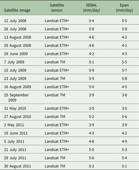
In the present study, 18 Landsat 5 Thematic Mapper ™ and Landsat 7 Enhanced Thematic Mapper (ETM)+ images were transformed into ETa maps. It is worth clarifying here that the use of different satellite images does not create any problem, because a radiometric calibration is performed and the respective calibration factors are available with each satellite image. Therefore, different satellite images provide the same remotely sensed data in terms of reflectance, since the band-widths of the various sensors used (Landsat 5–8) are identical and the estimated reflectance calculated refers to the same wavelength (by using the Relative Spectral Response filters for the specific satellite). Images were acquired for specific dates in the irrigation period of the crop being studied, which starts in mid-May and ends in mid-September. SEBAL was applied to the same satellite images; these estimations were subsequently compared with a direct evaporation measurement, namely that from an evaporation pan (Epan), which is hereby used as a reference. It was further examined to determine whether there was scope for increasing the algorithm's accuracy (D'Urso & Menenti Reference D'Urso, Menenti, Engman, Guyot and Marino1995; Kite & Droogers Reference Kite and Droogers2000). The results of this method refer to specific dates in the 4-year period 2008–2011.
Crop yield prediction
Crop production is also a basic element in the procedure for assessing water footprint, as mentioned in the definition. Earth observation tools can accurately predict the production of a whole region. The development of remote sensing techniques has provided the opportunity to optimize yields and to predict yield. Yield prediction plays a vital role in calculating water footprint and using real values obtained through remote sensing is preferable to using reference values for countries from FAO. This is very important in econometric or any other prediction models used for estimating water footprint because the use of average data reduces their accuracy. In this context, crop and soil parameters along with remotely sensed data can be used to develop models that can provide users with accurate yield estimations. Quantifying crop production at regional scales is critical for a wide range of applications and remote sensing offers great potential for monitoring regional production (Atzberger Reference Atzberger2013). In the present paper, knowledge of crop phenology was combined with multi-temporal imagery to estimate durum wheat crop yield (Atkinson et al. Reference Atkinson, Jeganathan, Dash and Atzberger2012; Meroni et al. Reference Meroni, Marinho, Sghaier, Verstrate and Leo2013) in southwest Cyprus. A semi-empirical model was developed to explore crop yield predictions. The spatial and temporal distributions of crop production derived in the present paper offer valuable information for agricultural management and policy.
Crop production is strongly related to numerous crop, meteorological and environmental factors. Field experiments from the early 1960s have shown that these factors affect the production of a crop proportionally (Quarmby et al. Reference Quarmby, Milnes, Hindle and Silleos1993), while new experiments have indicated the possibility of estimating crop yield by combining these factors along with remotely sensed data (Balaghi et al. Reference Balaghi, Tychon, Eerens and Jlibene2008; Atkinson et al. Reference Atkinson, Jeganathan, Dash and Atzberger2012; Bregaglio et al. Reference Bregaglio, Frasso, Pagani, Stella, Francone, Cappelli, Acutis, Balaghi, Ouabbou, Paleari and Confalonieri2015). Therefore, the purpose of the present study was to correlate basic factors that affect production of durum wheat using remote sensing and statistical analysis. The use of remote sensing has been proven effective in monitoring the growth of agricultural crops and in irrigation scheduling, and efforts have been made to develop various indices for different crops of different regions throughout the world (Balaghi et al. Reference Balaghi, Tychon, Eerens and Jlibene2008; Atkinson et al. Reference Atkinson, Jeganathan, Dash and Atzberger2012). The production and prediction of crop yield have a direct impact on year-to-year national and international economies and play an important role in food management (Hayes & Decker Reference Hayes and Decker1996).
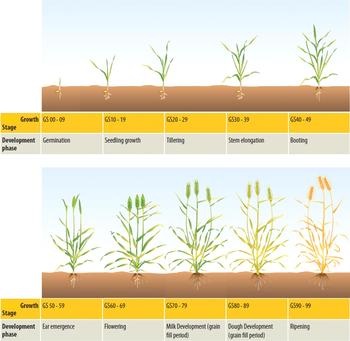
Several parameters, including crop temperature, soil moisture at a depth of 40 cm and LAI along with remotely sensed data (normalized difference vegetation index, NDVI) were statistically correlated to wheat production in the study area to identify whether durum wheat production can be estimated with sufficient accuracy and at which phenological stage this can be predicted. Recently, many studies have been performed to derive crop phenological stages based on satellite images. These studies aim to validate vegetation indices for monitoring the development of the phenological cycle from time series data. Sakamoto et al. (Reference Sakamoto, Yokozawa, Toritani, Shibayama, Ishitsuka and Ohno2005); Minacapilli et al. (Reference Minacapilli, Iovino and D'Urso2008) and Papadavid et al. (Reference Papadavid, Hadjimitsis, Toulios and Michaelides2011a) used time series of remotely sensed data to develop a new systematic method for detecting the phenological stages of different crops from satellite data, while Bradley et al. (Reference Bradley, Jacob, Hermance and Mustard2007) introduced a curve-fitting procedure to derive inter-annual phenologies from time series of noisy satellite NDVI data. Funk & Budde (Reference Funk and Budde2009) used an analogous metric of crop performance based on time series of NDVI satellite imagery. Ground spectro-radiometers have also been used to study the phenological cycle of groundnut (Papadavid Reference Papadavid2012; Papadavid & Hadjimitsis Reference Papadavid, Hadjimitsis, Hadjimitsis, Themistocleous, Michaelides and Papadavid2014). Papadavid & Hadjimitsis Reference Papadavid, Hadjimitsis, Neale and Maltese2009 and Papadavid et al. (Reference Papadavid, Hadjimitsis, Themistocleous, Toulios, Neale and Maltese2010, Reference Papadavid, Hadjimitsis, Perdikou, Michaelides, Toulios and Seraphides2011b) showed that field spectroscopy and empirical modelling, when successfully integrated, can develop new models of LAI and crop height during the phenological cycle of crops (Fig. 1).
Growth stages of cereals (source: GRDC Cereals Growth Stages Guide 2013).

Test site and examples
In the present paper, an example for each case will be illustrated to provide a method for estimating ETc and crop yield, basic elements in the procedure for calculating water footprint. In these examples, several steps must be followed in order to apply algorithms for ETc and crop yield estimation. As mentioned previously, these algorithms must be adapted to regional geo-meteorological conditions in order to increase the accuracy of results and enable users to employ them in their own regions. Hence, field measurements are conducted which are used to adapt algorithms to the regional conditions. The study area is traditionally agricultural with annual and perennial cultivations and is irrigated by Asprokremnos Dam, one of the biggest dams in Cyprus.
The area is almost at sea level (15 m a.s.l.) and characterized by a mild climate, which provides the opportunity for early production of leafy and annual crops. The uniform and moderate temperatures, attributed to the permanent sea breeze, and the relative humidity are conducive to early production of fruits and vegetables. Cereals are also cultivated in the area. A typical Mediterranean climate prevails, with hot dry summers from June to September and cool winters from December to March, during which much of the annual rainfall occurs (average 425 mm). The whole area is generally homogenous in terms of soil and morphology and the dominant soil type is the Cambisol (calcic and chromic types) (Papadavid Reference Papadavid2012).
In the present study, methods and algorithms were improved by introducing the necessary ground truth data into models. This means higher accuracy for the models but, crucially, the models are also adapted to local conditions. Models developed for other regions must be ‘localized’ before being applied to different regions. The methodology below explains the specific step, which provided accurate results at the end.
Regarding the examples provided for this purpose, groundnut was selected for estimation of ETc, while durum wheat was selected for crop yield estimation. These are two basic crops cultivated in the area of interest but are also major crops in Cyprus.
Materials and Methods
Evapotranspiration
The SEBAL algorithm takes into account crop canopy factors in order to estimate ETa. This provides the opportunity to feed the model with local data in an attempt to increase its effectiveness. Empirical equations using vegetation indices describing LAI and crop height could be included in the algorithm. The methodology adopted in the present study is based on the hypothesis that SEBAL's accuracy could be enhanced if the algorithm is supported with ground data regarding crop canopy factors and meteorological conditions of the area.
Spectroradiometric measurements
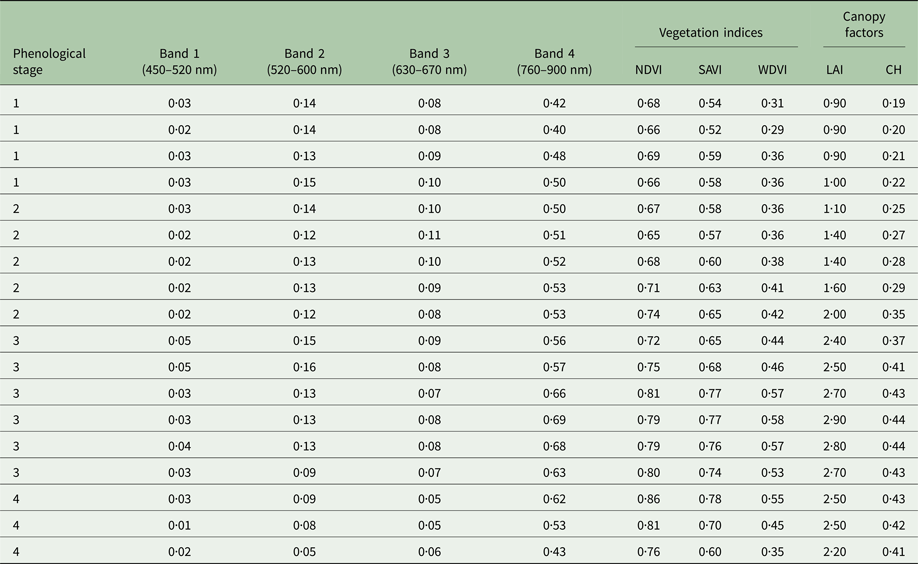
A 2-year (2009–2010 from April to July) field campaign was undertaken to collect spectral signatures of each crop included in the study. The aim was to obtain the reflectance of each crop during different phenological stages after the data were passed through relative spectral response filters (RSR). Field spectroradiometric measurements were made using a GER 1500 field spectroradiometer (Spectra Vista Corporation, Poughkeepsie, NY, USA) with reflectance spectrum from 350 to 1050 nm. The task was to estimate surface reflectance values equivalent to the Landsat TM/ETM+ bands 1, 2, 3 and 4 using the GER 1500 spectroradiometer in situ. To filter the data through the RSR values of Landsat TM/ETM+, GER 1500 reflectance values were interpolated to obtain reflectance values at the incremental wavelength of the RSR. The initial spectroradiometric measurement was taken when each crop had enough foliage (27 days after they were planted) to avoid soil effects on spectroradiometric data, while the final measurement was taken just after the crop started drying and became yellowish as shown in Table 1.
Spectroradiometric data, vegetation index and crop canopy factors during different stages of crop development (the phenological stages are: 1 = vegetative, 2 = flowering, 3 = yield formation, 4 = ripening)

NDVI, normalized difference vegetation index; SAVI, soil-adjusted vegetation index; WDVI, weighted difference vegetation index; LAI, leaf area index; CH, crop height.
Leaf area index and crop height measurements
Measurements for LAI and crop height were taken at the same time as spectroradiometric measurements, following the same phenological cycle of each crop for the corresponding cultivating periods. The purpose was to create time series of these two parameters and correlate them to vegetation indices (Baret et al. Reference Baret, Hagolle, Geiger, Bicheron, Miras, Huc, Berthelot, Nino, Weiss, Samain, Roujean and Leroy2007).
Vegetation indices
Time series of vegetation indices were created based on the spectroradiometric reflectance of each crop in each phenological stage. Vegetation indices have been widely used for assessing vegetation condition, cover, phenology and various processes such as evapotranspiration, climate- and land-use-change detection and drought monitoring (Haboudane et al. Reference Haboudane, Miller, Pattey, Zarco-Tejada and Strachan2004; Glenn et al. Reference Glenn, Huete, Nagler and Nelson2008). The spectral vegetation index was correlated to LAI and then to crop height. NDVI, soil-adjusted vegetation index (SAVI) and weighted difference vegetation index (WDVI) were the selected indices. Such indices are widely used in various evapotranspiration algorithms and models (Bannari et al. Reference Bannari, Morin, Huette and Bonn1995).
Modelling leaf area index and crop height in terms of vegetation indices
Different models were tested in order to identify the one that best described LAI and crop height in terms of vegetation index. The fact that there is no universal equation relating LAI to a vegetation index (Qi et al. Reference Qi, Kerr, Moran, Weltz, Huete, Sorooshian and Bryant2000) forces those using remote sensing to develop equations for each crop under the current relevant conditions, using measurements of LAI and remote sensing data, such as spectroradiometric measurements. As a result, each image must be transformed into an LAI map. Factors such as soil characteristics, atmospheric effects and topography, which affect vegetation index, must be considered and their impact minimized in this procedure; thus, improved vegetation indices such as SAVI and WDVI were used for this purpose. In the present modelling procedure, an attempt has been made to model LAI and crop height in terms of one of the three vegetation indices mentioned earlier (i.e., NDVI, SAVI and WDVI). The models for LAI used in the present study are mathematically expressed as linear, exponential logarithmic and polynomial. The independent variable is one of the vegetation indices and the dependent variable is one of the factors (e.g. LAI or crop height) that the user wishes to correlate to vegetation indices.
Mapping leaf area index and crop height
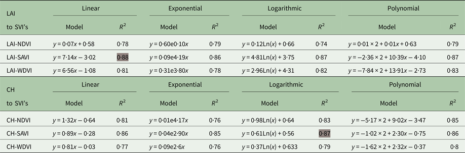
The two crop canopy parameters were mapped using the ERDAS Imagine software (http://www.hexagongeospatial.com/products/power-portfolio/erdas-imagine). The satellite images were transformed into maps in order to: (1) test the models in practice and (2) be able to insert them as inputs to the evapotranspiration algorithms. In order to reveal the strongest relationship, time series of the required parameters must be created and statistical methods used to create empirical models to characterize LAI and crop height as shown in Table 2.
Results of the correlation analysis for leaf area index (LAI) and crop height (CH) to vegetation index (VI)

Grey shading = model with the highest R 2.
Application of the surface energy balance algorithm for land algorithm
Modified by empirical equations, SEBAL is applied in order to estimate actual ETc. It is essentially a single source model that solves the energy balance equation and provides maps of ETa on a pixel basis. Modified SEBAL with adopted crop canopy equations is hereafter termed ‘CY-SEBAL’, which implies reference to the conditions in Cyprus.
Effectiveness of the proposed method
The proposed method's effectiveness is assessed using Epan data for the same dates as the satellite images. A t-test was employed to evaluate results and cross-check if there is significant statistical difference between the SEBAL results.
Crop yield
The purpose of the methodology developed for the present study was to estimate and map crop production (yield). Remote sensing vegetation indices, crop canopy and meteorological factors are vital elements in this procedure and were measured for statistical regression to durum wheat yield.
Normalized difference vegetation index was inferred from in situ measurements using a hand-held field spectroradiometer (GER 1500) and the data filtered through RSR filters, as described by Papadavid (Reference Papadavid2012). Simultaneously, direct measurements were also taken for LAI, soil moisture and crop temperature. Time series of these were created and used to model crop production/yield using statistical methods. After applying the required statistical methods, the best model based on the determination factor (r 2) and ANOVA results (F test), were applied to:
(a) verify the model itself and
(b) to map crop production of durum wheat in the study area. The entire methodology is described in detail below.
Spectroradiometric in situ measurements
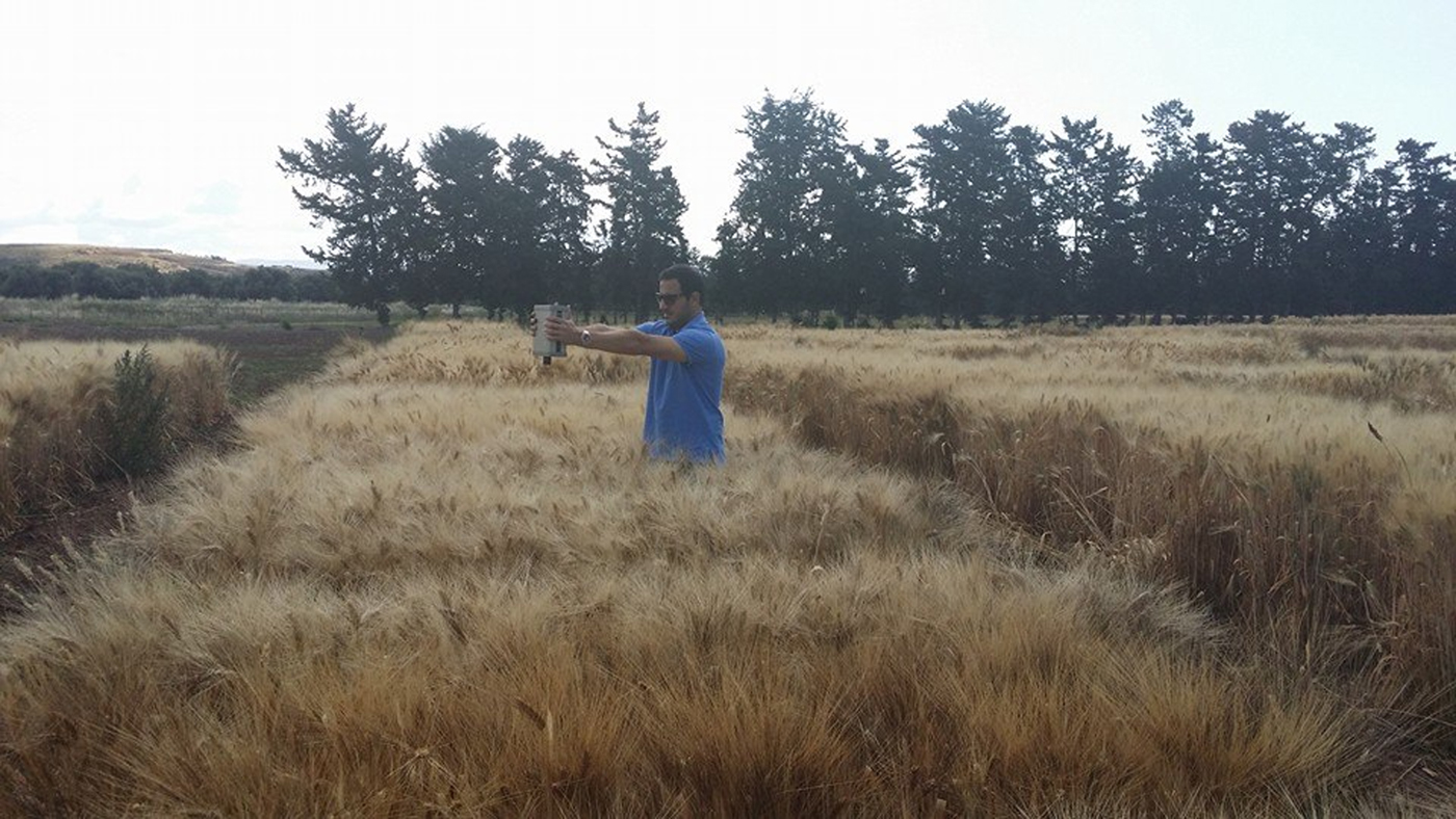
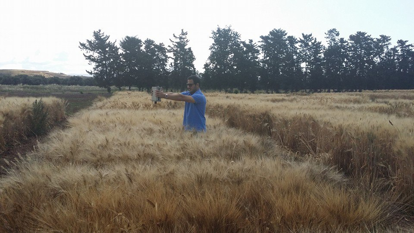
A 3-year field study (2009–2011) was undertaken to collect the spectral signatures of durum wheat from 15 different plots in the study area (Fig. 2). Three phenological stages (Fig. 1) were followed to test whether it is possible to estimate crop yield prior to harvest. The phenological stages followed were (a) tillering-stem elongation period, (b) flowering period and (c) grain filling period, in order to calculate the mean reflectance of each phenological stage, as indicated by Papadavid (Reference Papadavid2012).
In situ spectroradiometric measurements.
Leaf area index, crop temperature and soil moisture at 40 cm in situ
Measurements of LAI, crop temperature and soil moisture at a depth of 40 cm were taken at the same time as spectroradiometric measurements and following the same phenological cycle of each crop for the corresponding cultivating periods. The purpose of this was to create time series of these parameters corresponding to each spectroradiometric measurement that will be correlated to crop yield. Using the SunScan canopy analyser (Delta-T Devices Ltd., UK), users can acquire the LAI value directly by setting the machine up perpendicular to the crop rows (Stancalie et al. Reference Stancalie, Nertan, Toulios, Toulios and Stancalie2010). Also, a calibration measurement above the canopy is required each time the user takes a measurement in the crops. The SunScan was calibrated under a standard light source against an accurate PAR (Photosynthetic Active Radiation) quantum sensor. The spectral and cosine responses of the sensors approximate to the ideal response, but fall off at the extremes of the range. Under most normal daylight conditions, errors due to the deviation are small, but it is possible, in conditions such as under artificial light, to find larger errors in the absolute values measured. Since the Sunshine Sensor and Probe of the SunScan are closely matched, this has a minimal effect on the canopy calculations, which are based on ratios of incident and transmitted light (Lambert et al. Reference Lambert, Peeters and Toussaint1999). Crop temperature (CT) was derived from a digital hand-held thermometer while soil moisture (SM) was derived from a WET-2 soil moisture meter (Delta-T Devices, Cambridge, UK). These measurements were taken simultaneously with the random spectroradiometric measurements and an average value for each parameter was derived for each day and each plot. The measurements were then averaged for the three phenological stages.
Crop yield
The real crop yield (CY) for the specific 15 plots studied was obtained from the Agricultural Research Institute (ARI). It was then linearly regressed to these factors (NDVI, LAI, crop temperature and soil moisture) for each of the 3 years and stages, in the form of [CY = a + b(NDVI) + c(LAI) + d(CT) + e(SM)] to test whether there was any statistically significant relationship between the four independent parameters and CY (dependent parameter). This method was used as an indicator for strong correlations with particular phenological stages, and then all measurements of each stage were grouped together, resulting in 45 measurements for each stage. This was the final dataset to run against the regression analysis for those phenological stages indicated to have good correlation. Therefore, the regression was run for each stage of each year to identify which particular phenological stage had a strong correlation. The stage with the best R 2 was selected. Then, having a satellite image and values of soil moisture, crop temperature and LAI, one can derive the yield of durum wheat using the specific model.
Pre-processing of satellite images
Geometric rectification and radiometric correction including atmospheric correction of satellite data were applied before main processing of the data. Pre-processing is essential and comprises a series of sequential operations such as atmospheric corrections, image rectification and registration and masking. At the time, only Landsat 7 ETM+ and Landsat 8 OLI images were available, with resolution of 30 m. Red and infrared bands (bands 3 and 4 for Landsat 7ETM+ and bands 4 and 5 for Landsat 8 OLI) were used to infer NDVI. All satellite images used for the present study have undergone radiometric and geometric corrections. Regarding radiometric corrections, the images were transposed from DN (digital numbers) into radiance and then to reflectance by applying the necessary equation and using ERDAS Imagine software. Atmospheric corrections were also applied to the satellite images in order to remove atmospheric effects. The darkest pixel algorithm was employed and applied to all images. Radiometric corrections of remotely sensed data aim to remove effects originating from the building of the sensor and effects from the atmosphere. The consideration of these effects is very important (Papadavid et al. Reference Papadavid, Hadjimitsis, Perdikou, Michaelides, Toulios and Seraphides2011b).
Mapping durum wheat yield using the specific algorithm
Satellite images were used in order to map yield. Crop yield was mapped using ERDAS Imagine and the proposed algorithm, which is based only on image characteristics. The satellite images were transformed into maps to test the models and to have an area map of durum wheat. Four different maps (NDVI, crop temperature, LAI and soil moisture) were produced in a methodological order to form the specific algorithm for estimating CY. These maps were amalgamated into one single map (the fifth map), illustrating durum wheat yield in tonnes/ha. Since the method refers to ‘image-based method’, all dependent variables of the model must be found from specific parameters in satellite images.
The purpose then is to estimate all models’ parameters using only remotely sensed data. Thus, the user needs to develop maps from the satellite imagery which will be used as inputs in the algorithm in a certain order as explained below:
(i) An NDVI map is produced directly from the satellite images, using the near-infra-red (NIR) and infra-red (IR) bands of the satellite. The NDVI is considered to be a useful index for crop yield assessment models using various approaches from simple integration to more complicated transformation. It reflects vegetation greenness; thus it indicates the health of vegetation and is an integral part of the model. It is the most known and widely used ratio-based index:
where NIR is the reflectance of the near-infrared band, and RED is the reflectance of the visible red band. The range is from –1 to +1, with negative values representing non-vegetated areas, while positive values represent vegetated area. $${\rm NDVI} = \displaystyle{{{\rm NIR} - {\rm R}} \over {{\rm NIR} + {\rm R}}}$$
(ii) LAI map. The following equation was applied to estimate LAI (Quarmby et al. Reference Quarmby, Milnes, Hindle and Silleos1993; Hadjimitsis et al. Reference Hadjimitsis, Clayton, Retalis and Spanos2000):
$${\rm LAI} = \displaystyle{{ - 1} \over \alpha} \ln \left( {1 - \displaystyle{{{\rm WDVI}} \over {\rho _\infty \left( {\lambda _{{\rm NIR}}} \right)}}} \right)$$


where LAI = leaf area index, WDVI = weighted difference vegetation index, α = complex combination of extinction and scattering coefficients, and ρ ∞ = asymptotically limiting value of the WDVI at very high LAI values.
Standard values for α and ρ ∞ were taken from the literature specifically for cereals (Agapiou et al. Reference Agapiou, Papadavid, Hadjimitsis, Neale and Maltese2009).
As WDVI is a distance-based index, relatively better atmospheric correction needs to be applied to the data, which is not necessary for ratio-based indices such as NDVI and SAVI. However, as mentioned previously this limitation is bypassed using a spectroradiometer. The WDVI is defined as follows (Papadavid et al. Reference Papadavid, Hadjimitsis, Themistocleous, Toulios, Neale and Maltese2010):
 $${\rm WDVI} = {\rm NIR} - \gamma {\rm R}$$
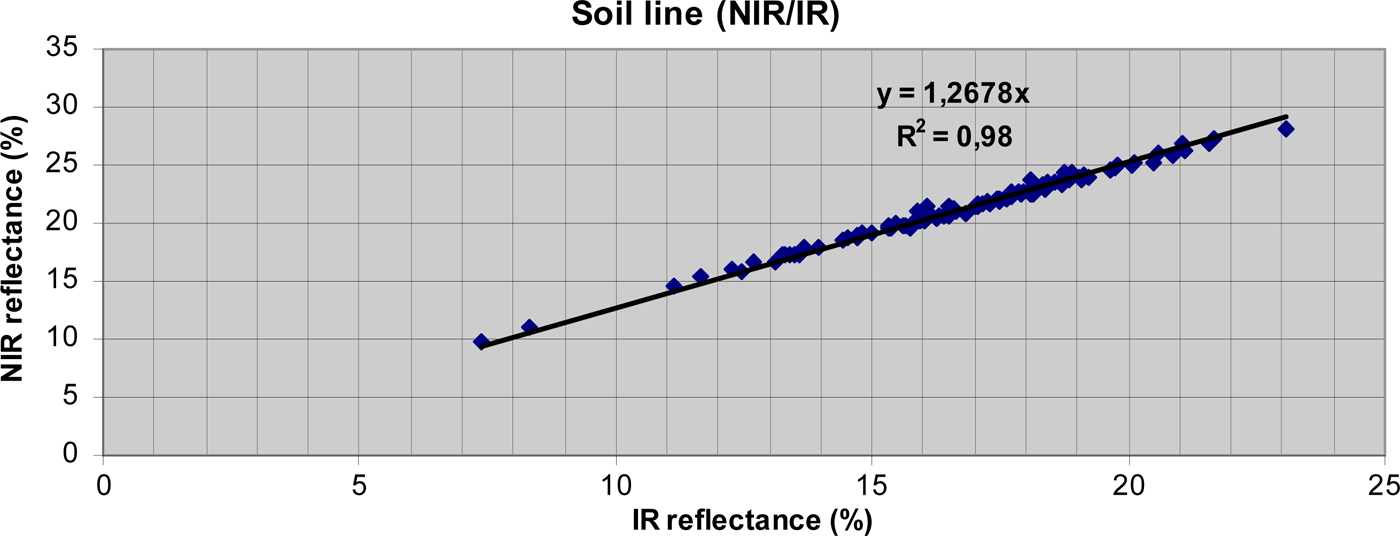
where NIR is the reflectance of the near-infrared band, RED is the reflectance of the visible red band and γ is the slope of the soil line (Papadavid et al. Reference Papadavid, Hadjimitsis, Perdikou, Michaelides, Toulios and Seraphides2011b). The WDVI index has the advantage of greatly reducing the influence of soil background on the surface reflectance values. Although simple, WDVI is as efficient as most of the slope-based vegetation indices. The effect of weighting the red band with the slope of the soil line is the maximization of the vegetation signal in the near-infrared band and the minimization of the effect of soil brightness. The slope line was created from the NIR and R spectrum using spectroradiometric data (200 random measurements, taken throughout the year) from bare soil within the study area, and set at 1·27 (Fig. 3).
Soil slope line of the area of interest from spectroradiometric measurements of the area. NIR, near infrared; IR, infrared.

The specific equation was applied to satellite images and LAI maps were created. Various studies have shown that empirical equations of LAI and vegetation index can provide good estimates of LAI from the satellite images (Quarmby et al. Reference Quarmby, Milnes, Hindle and Silleos1993; Lambert et al. Reference Lambert, Peeters and Toussaint1999; Hadjimitsis et al. Reference Hadjimitsis, Clayton, Retalis and Spanos2000).
(iii) Crop temperature map. In the pre-processing procedure, the thermal band also undergoes radiometric correction in order to be used. Crop temperature is obtained directly from the thermal bands of the satellites (Landsat 7 ETM+ and 8 OLI).
(iv) Soil moisture (SM) map. The basic principle of thermal infra-red (TIR) methods is that land surface temperature is sensitive to surface soil water content due to its impact on surface heating process (heat capacity and thermal conductivity) under bare soil or sparse vegetation cover conditions (Zhao & Li Reference Zhao and Li2013). The common scheme most often utilized in TIR remote sensing of SM is to decouple the surface thermal properties from ambient temperature (daily temperature cycle) by calculating the thermal inertia (Minacapilli et al. Reference Minacapilli, Agnese, Blanda, Cammalleri, Ciraolo, Urso, Iovino, Pumo, Provenzano and Rallo2009; Qin et al. Reference Qin, Yang, Lu, Chen, Zhao and Han2013; Lei et al. Reference Lei, Bian, Daniels and Liu2014). Thermal inertia essentially describes a physical property that characterizes the surface resistance to ambient temperature change (Soliman et al. Reference Soliman, Heck, Brenning, Brown and Miller2013). Provided that parameters related to the atmosphere and meteorological conditions have been accounted for, surface temperature (T s) is primarily dependent upon the thermal inertia of the soil. Thermal inertia, in turn, is dependent upon both thermal conductivity and heat capacity, which increase with soil moisture (Price Reference Price, Williamson and Stein1992). Therefore, for the specific case where land is covered by vegetation, soil moisture is directly correlated to crop-land thermal inertia using a simple model from NASA (NASA 1978), based on the assumption that the sun produces a periodic heating of the terrestrial surface and the loss of heat from the ground is caused entirely by radiative transfers. The equation states:
$${\rm S} = {\rm A} \times {\rm S} + ({\rm 1} - {\rm A}) \times {\rm S}$$

where S is the solar energy incident on a surface of albedo A. The quantity of heat absorbed by the surface, [(1−A) × S], determines an increase of the surface temperature and the amount of such increase (ΔT) depends on thermal inertia. Introducing apparent thermal inertia (ATI) (NASA 1978; Price Reference Price, Williamson and Stein1992) as an approximate thermal inertia value and considering an area with uniform solar energy, the following relationship is obtained:
 $${\rm ATI} = \displaystyle{{({\rm 1} - {\rm A})} \over {\Delta {T}}}$$
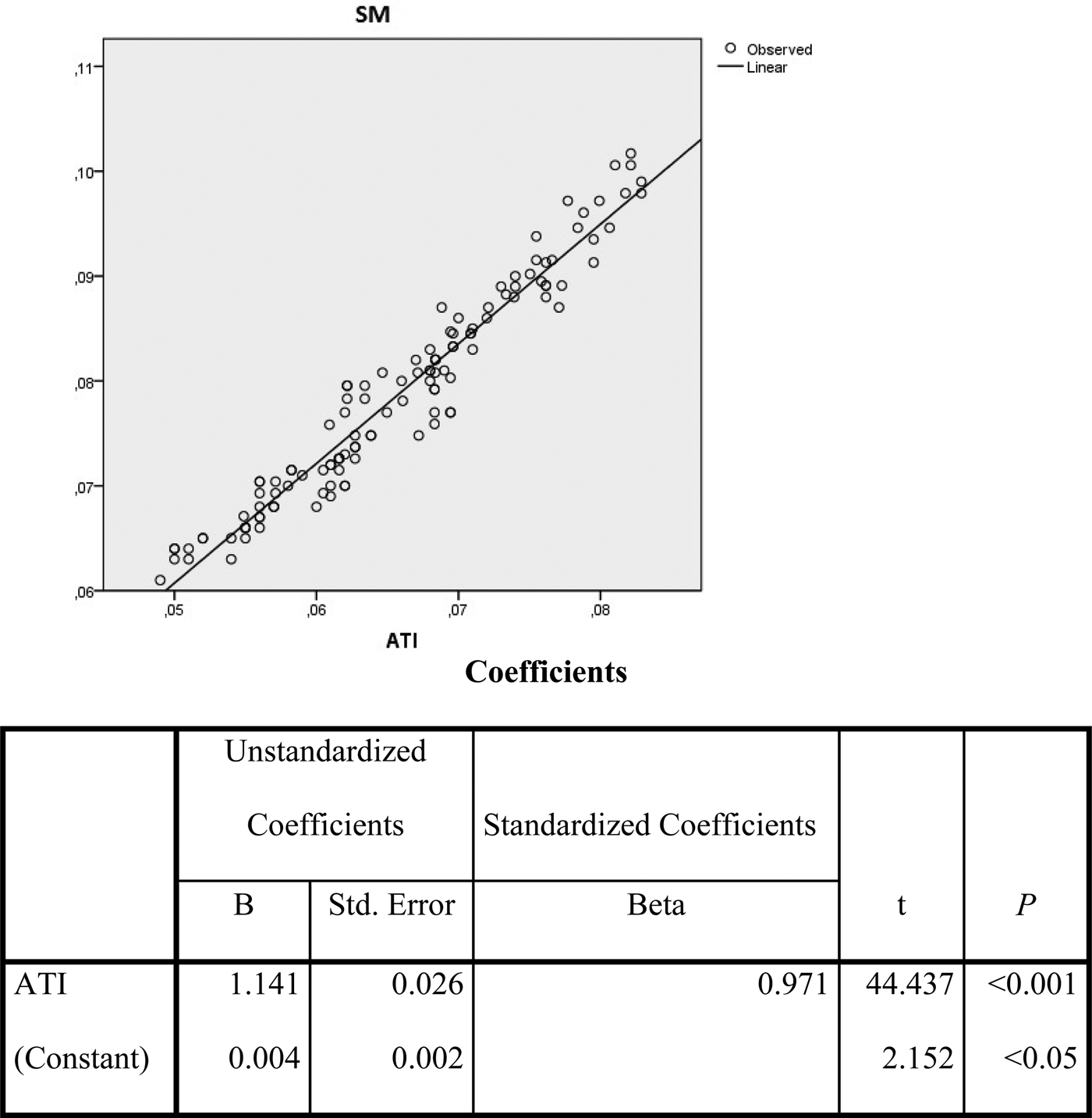
where ΔT can be assumed as the difference between the maximum (T max) and the minimum (T min) value that the surface temperature assumes during the diurnal cycle. As such, the units for ATI as ‘per Kelvin’ (/K). Using the GER 1500 for retrieving albedo and the digital hand-held thermometer for estimating ΔT, ATI was estimated for every day of the specific phenological stage (grain filling), which is about 40 days, during the 3-year study period. It must be mentioned that there was little or no rain during this specific period. Direct measurements of soil moisture were taken simultaneously, at the same plots cultivated with durum wheat. Therefore, chronological time series of these two parameters were developed in order to test correlations. The following linear equation (Fig. 4) reveals the strong relation between the two parameters, as also shown by Carlson (Reference Carlson1986) and Tramutoli et al. (Reference Tramutoli, Claps, Marella, Pergola, Sileo, Mugnai, Guzzetti and Roth2000):
 $${\rm SM} = 0{\cdot}004 + 1{\cdot}14({\rm ATI})$$
The specific equation developed by the current authors has a very strong R 2 reaching 0·92 and it will be used to estimate soil moisture from the satellite images directly. This enables users to avoid direct point measurements of soil moisture and create soil moisture maps at the area of interest.
Apparent thermal inertia (ATI) to soil moisture (SM) correlation.

Algorithm verification
After inferring the best model describing crop yield, the procedure was evaluated. A different period from the research years (2012–2014 v. 2009–2011) was chosen for the validation. This was vital since the model will be used in the future and in different plots. Crop yields, provided by the durum wheat producers (owners of the plots) were compared to the predicted crop yield measurements arising from the algorithm application found in the previous step ([CY = a + b(NDVI) + c(LAI) + d(CT) + e(SM)]) after mapping the crop yield. The Student's t-test for paired samples, as a statistical significance test, was applied to compare and assess the results. To assess the value of t, the standard deviation SD of each pair of values (real and predicted) must be known. Variance  $(S_D^2 )$ is calculated from the equation:
 $$S_D^2 = \displaystyle{{\left[ {\Sigma D_j^2 - ({(\Sigma D_j)}^2/n)} \right]} \over {n - 1}}$$
where D j refers to the difference of each pair and n is the number of the pairs. The average Variance  $(S_{Da}^2 )$ of all pairs must then be calculated using the following equation
 $$S_{Da}^2 = \displaystyle{{S_D^2} \over n}$$
where D a is the average difference of each pair Finally, the t value is calculated by solving the equation:
 $$t = \displaystyle{{Da} \over {S_{Da}}}$$
Results
Evapotranspiration
It is noticeable that in SEBAL, empirical equations are used to describe parameters that need to be measured directly. The intended purpose is to include required local empirical equations in the algorithm and check whether the accuracy can be enhanced. In this respect, the current work has been able to develop empirical equations, adapted to the Cypriot (Mediterranean) conditions, and embed them in the algorithm, in an attempt to make the results as accurate as possible. The results from SEBAL are compared with those of the reference method measurements derived from the same plots.
Modelling leaf area index and crop height with vegetation indices
The use of vegetation indices to statistically describe LAI and crop height is common in international literature and many empirical models are available depending on the conditions and location (Running & Coughlan Reference Running and Coughlan1988; Clevers Reference Clevers1989; Tiktak & Van Grinsven Reference Tiktak and Van Grinsven1995). Time series of LAI, crop height and vegetation index (i.e., NDVI, SAVI and WDVI) were created in order to proceed with correlations (Table 1).
Leaf area index is used in the SEBAL algorithm to estimate the surface emissivity, which are used in turn to infer the surface temperature from the thermal band (band 6) of the Landsat satellite in order to calculate net radiation (R n).
Leaf area index, defined as the ratio of the total area of all leaves of a plant to the ground area of the plant (see Watson Reference Watson1947), is related to SAVI in the classic SEBAL as shown below:
 $${\rm LAI} = - \displaystyle{{\rm ln(0{\cdot}69 - {\rm SAVI}/0{\cdot}59)} \over {0{\cdot}91}}$$
The whole procedure of statistically describing LAI in terms of vegetation index in the present work is presented in Table 2. Linear, exponential, logarithmic and polynomial models were used to infer the best-fitting model under the current conditions. Using empirical modelling techniques and field spectroradiometric data, it was found that the coefficient of determination obtains the highest value (R 2 = 0·88) when LAI is correlated to SAVI. In order to be as accurate as possible, the measurements for both LAI and crop height were taken following the phenological stages of groundnut. The mathematical model used to describe LAI in terms of SAVI is:
 $${\rm LAI} = {\rm 7}.{\rm 99} \,\,({\rm SAVI})- {\rm 3}{\cdot}{\rm 29}$$
Crop height is used to infer the momentum roughness (Z om), in order to estimate friction velocity and thus the aerodynamic resistance to heat transport, which is a basic element for Sensible Heat Flux (Santos et al. Reference Santos, Lorite, Allen and Tasumi2012). In classic SEBAL, Z om is found using the empirical relationship:
 $$Z_{{\rm om}} = 0.{\rm 12\,crop}\, {\rm height}$$
where crop height is set to a standard height, usually between 0·25 and 0·30 cm, or by utilizing an LAI map.
In the present research, the above equation was modified using a vegetation index to estimate crop height and create a map of Z om, which was subsequently used as an input in the algorithm describing the whole area. Following the same procedure as for LAI, crop height was described in the present research using SAVI as follows:
 $${\rm Crop}\, {\rm height} = 0.{\rm 65\,ln}({\rm SAVI}) + 0{\cdot}{\rm 62}$$
This is the relationship in Table 2, having the highest coefficient of determination (R 2 = 0·87).
By adopting the above logarithmic model, Eqn (6) was subsequently transformed to:
 $$Z_{{\rm om}} = 0{\cdot}0{\rm 7\,ln}\,({\rm SAVI}) + 0{\cdot}{\rm 34}$$
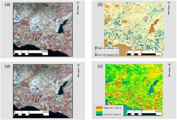
Equations (5) and (7) are used to calculate LAI and crop height, respectively, with the use of satellite data. These equations were input to the ERDAS Imagine software (Modeler module), in order to create LAI and crop height maps (Fig. 5). These maps are the satellite images transformed to pixel-based maps, where users can retrieve the values of the two specific parameters, LAI and crop height. The specific rasters are used as inputs in the SEBAL algorithm. It should be noted that since the equations refer to groundnut, they should be used exclusively for this specific crop and not for any other.
Generation, using Landsat image (a), of (b) leaf area index (LAI) and (c) crop height (CH) maps (in pseudo colour).

Since SAVI is the vegetation index that was found to best fit both models, it is useful to briefly address this particular vegetation index. It is described by the following equation:
 $${\rm SAVI} = \left[ {\displaystyle{{{\rm NIR} - {\rm R}} \over {{\rm NIR} + {\rm R} + {\rm L}}}} \right]({\rm 1} + {\rm L})$$
where NIR is the reflectance value of the near-infrared band, R is reflectance of the red band, and L is the soil brightness correction factor.
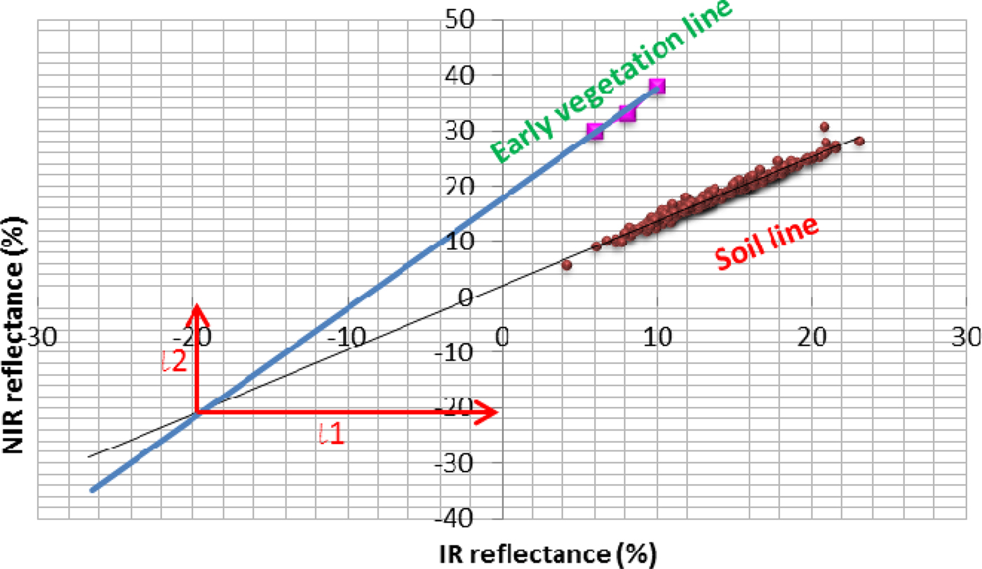
SAVI was adapted to the local conditions with the custom soil-adjustment constant L set, using >250 ground spectroradiometric measurements in the years 2009–2010 (Fig. 6); L is the sum of l 1 and l 2 (the co-ordinates of the point, where Early Vegetation Line and Soil Line are intersected), as described by Huete (Reference Huete1988). Indeed, L is basically the offset of the NIR/IR (near infrared/infrared reflectance) and is set to a value of 0·41, as determined from Fig. 6. When semi-empirical models are retrieved from the statistical analysis, then LAI and crop height maps are created using the available satellite images.
Adapting soil-adjusted vegetation index (SAVI) to ground conditions. Employing the modified Surface Energy Balance Algorithm for Land (SEBAL) model. NIR, near infrared; IR, infrared.

Maps of ETa were finally created for each satellite image, using the empirical Eqns (5) and (7). These maps were employed to infer the ETa of groundnut for all the available images from Landsat 5 and 7 satellites. The value of ETa refers to the mean value of the four plots of groundnut in the study area that follow the same phenological cycle and are subject to the same meteorological conditions. ETa values for groundnut were compared to the Epan values provided by the ARI of Cyprus. The ARI has the resources for estimating ETa by using Epan data collected since 1978 (Metochis Reference Metochis1997).
As can be inferred from Table 3, the results of the two methods applied are very close. It is noteworthy that results from SEBAL follow the same variations as results of the direct Epan method, implying that when the Epan results decrease or increase, there is a respective decrease or increase in the results of SEBAL. The Epan method was used here as a preliminary tool to assess the effectiveness of the revised proposed SEBAL method, despite the fact that Epan refers to point measurements of ETa. The average deviation of SEBAL with respect to Epan reaches 1·9%.
Surface Energy Balance Algorithm for Land (SEBAL) and evaporation pan (Epan) measurements

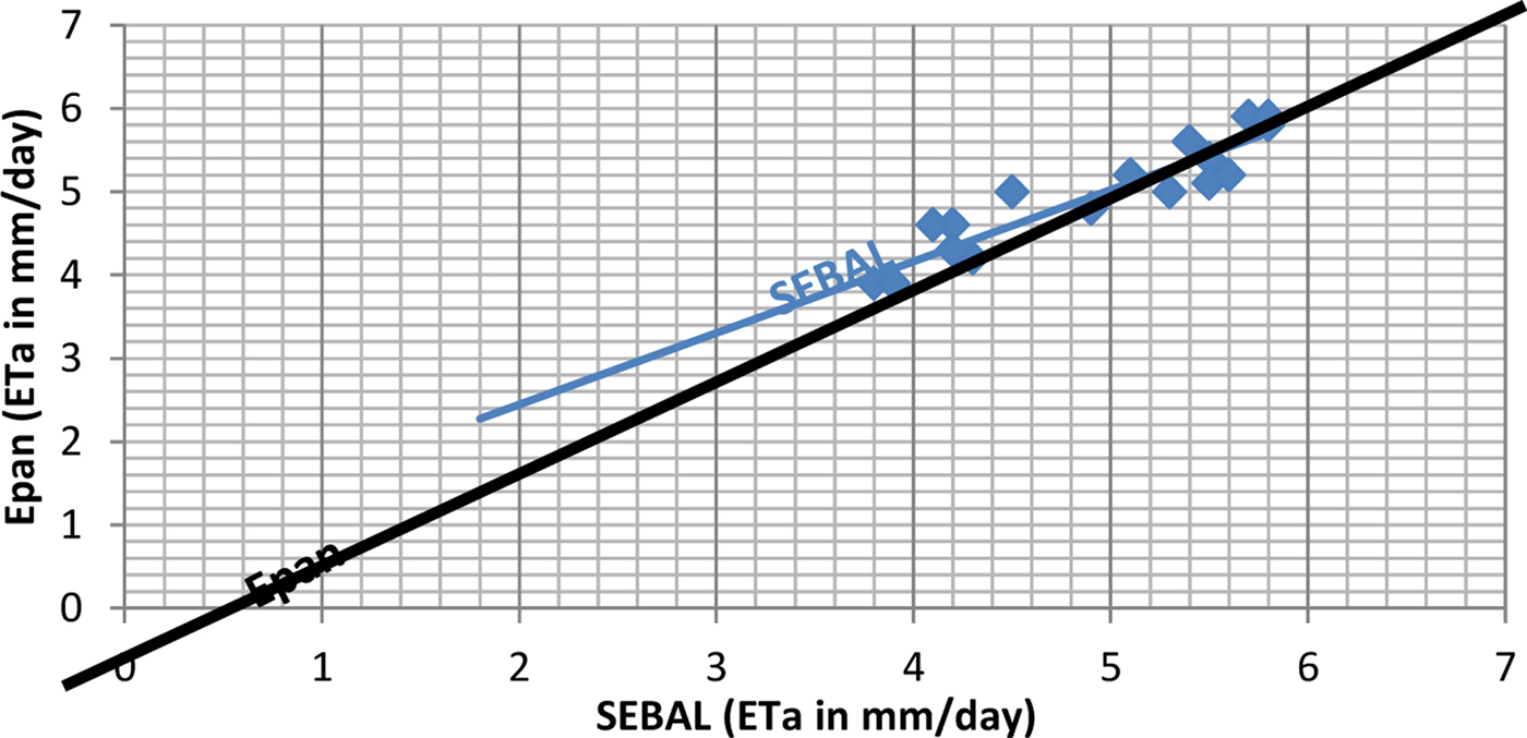
Figure 7 depicts graphically the results of using the two methods (SEBAL v. Epan method) for calculating evapotranspiration. Although it can clearly be inferred that the results are very close, it is considered important to substantiate this by using appropriate statistical testing. To this end, a t-test was performed. The t-test results are shown in Table 4, revealing that SEBAL results in mm/day are not significantly different (P < 0·05) from the Epan method results.
Graphical results for evaporation pan (Epan) v. Surface Energy Balance Algorithm for Land (SEBAL). ETa, actual evapotranspiration.

t-test analysis (P < 0·05)

Epan, evaporation pan.
Crop yield
The entire methodology intends to estimate durum wheat yield before harvest, in order to have a yield projection so that policy makers can make appropriate decisions regarding the crop based on sound scientific data. The study combines a statistical method along with remote sensing techniques to map crop yield on satellite images and retrieve the necessary data on durum wheat yield. At this point, the algorithm relates only to durum wheat and cannot be used for any other crops.
Crop and meteorological time series
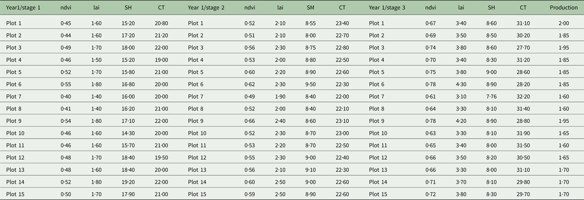
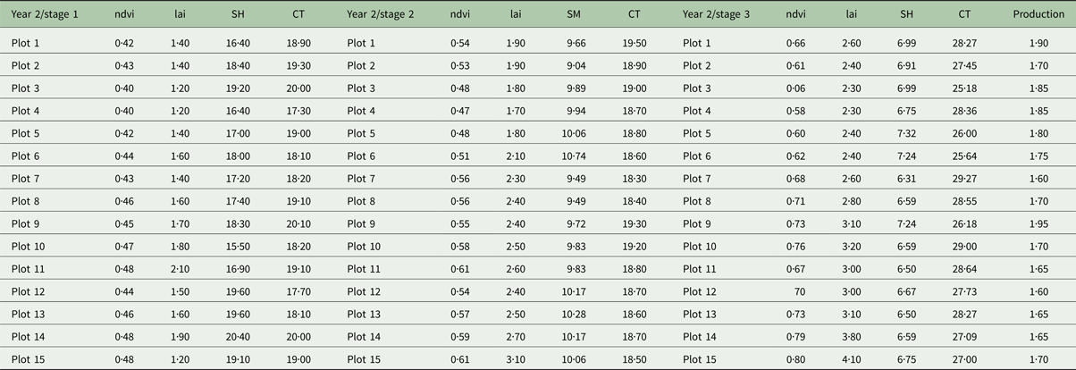
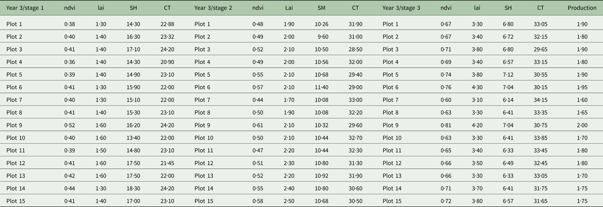
After the ground truth data were collected and averaged into the three phenological stages (namely stage 1, tillering-stem elongation; stage 2, flowering; and stage 3, grain filling), time series of each factor were created in order to check their correlation with durum wheat production. Fifteen plots in the study area were plotted for their NDVI (unitless), LAI (m2/m2), SH (%) and CT (°C) for 3 years as shown in Tables 5–7. Each sub-table contains the three phenological stages selected for the study while at the end of each sub-table the specific year's production appears.
Results of Year 1 of the three stages for normalized difference vegetation index (NDVI), leaf area index (LAI), soil moisture (SM) and CT. Year's 1 production is shown in the last column

Results of Year 2 of the three stages for normalized difference vegetation index (NDVI), leaf area index (LAI), soil moisture (SM) and CT. Year's 2 production is shown in the last column

Results of Year 3 of the three stages for normalized difference vegetation index (NDVI), leaf area index (LAI), soil moisture (SM) and CT. Year's 3 production is shown in the last column

As indicated, for each year NDVI, LAI and CT increase from stages 1 to 3, which is expected since plants were actively growing and covering more soil, resulting in increased LAI and NDVI, which denotes the proportion of vegetation in a pixel.
The CT increases in spring and summer due to higher incoming solar radiation (energy), which is also the cause of the reduction in soil moisture. The explanation is similar to the above for the increase of CT. Increased sun energy increases evaporation through the soil, leading to decreased moisture in the soil, but also in the crops’ water absorption. The above phenomena take place in the same sequence for the 3 years of study for all the factors as described above. In the last column, each plot's production (t/ha) is indicated (Tables 5–7).
Regression analysis results
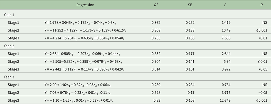
As mentioned previously, after inferring the necessary data to develop the image-based algorithm for estimating durum wheat yield, regression analysis was employed to find out whether there was any statistical relation between selected independent variables (NDVI, LAI, SM and CT) and CY (dependent variable) and, if there was any strong relationship, in which time-window this relationship is best to be considered for estimating the yield. Thus, the temporal and statistical aspects of the proposed algorithm were examined. Regression analysis (Table 8) revealed that there is a possibility for a fine model, which can describe yield through NDVI, LAI, SM and CT, especially for the phenological stages of flowering and grain filling (stages 1 and 2). For the first year, a very strong coefficient of determination (R 2) was observed for stages 2 and 3 reaching 0·808 and 0·755, respectively. For the second year, R 2 was high for stages 2 and 3, reaching 0·704 and 0·614, respectively. It worth noting that, for these 2 years, stage 2 had a higher R 2 than stage 3, while for the third year there was again strong R 2 but that stage 3 had a higher R 2 than stage 2. For all 3 years, the R 2 in stage 1 was below the permissible limits (~0·6) for considering the model as valid for estimating yield.
Regression analysis results for each year and each stage

At this stage, it is unclear whether stage 2 or 3 should be used for developing a model regarding yield estimation. Inevitably, data from stage 2 and simultaneously data from stage 3 of the 3 years must be combined (3 years × 15 plots = 45 measurements of each parameter) in order to develop new models with more data to have a better statistical meaning. Thus, time series of the 3 years for stages 2 and 3 were created and the same methodology was followed to develop new models and choose the stage of durum wheat where one should apply this method for estimating yield. The results of the new regression analysis are shown in Table 9.
Regression analysis results for combined data of stages 2 and 3

The results confirm that the best stage for applying the method for estimating durum wheat yield is at the grain filling (stage 3), with a very high R 2 of 0·886. This high level of correlation indicates that the independent variables can explain 89% of the dependent variable with standard error (s.e.) of estimate of 0·12, which is very low. The F statistic value is 9·085, indicating that the overall regression model has a good fit for the data since the observed F(9·085) value is higher than the statistic (F 4,45 = 5·7) for P < 0·05. Significance of P < 0·01 suggests that, overall, the model applied can statistically significantly predict the outcome variable. This means that the prediction model is very accurate and crop yield can be calculated from the independent parameters NDVI, LAI, SM and CT. The model developed from this regression analysis using the above steps is the following:
 $$Y = - 0{\cdot}{\rm 92} + 0{\cdot}{\rm 37}x_{\rm 1} - 0{\cdot}0{\rm 8}x_{\rm 2} + 0{\cdot}{\rm 62}x_{\rm 3} - 0{\cdot}0{\rm 1}x_{\rm 4}$$
where Y = Production, x 1 = NDVI, x 2 = LAI, x 3 = Soil moisture (depth of 40 cm), x 4 = Crop temperature, stage 1: tillering-stem elongation, stage 2: flowering, and stage 3: grain filling.
Regarding R 2 of the second stage, flowering, the results have shown a rather poor relationship which has rejected the model and the time-window of this stage, though there was a strong R 2 individually for the years 2009 and 2010.
The results of regression analysis assisted in the procedure for mapping durum wheat yield in the study area. Three Landsat Images of 2012 (Landsat 7 ETM+ 29/4/2012), 2013 (Landsat 8 ETM+ 4/5/2013) and 2014 (Landsat 8 ETM+ 2/5/2014), all referring to the grain filling stage, were used to apply the semi-empirical model into the images. Thus, thematic yield maps were created by applying the specific algorithm, so as to retrieve values of crop yield for all the plots in the area of interest cultivated with durum wheat. In the maps developed using the specific procedure each pixel in the map has a value that represents the durum wheat production. These maps are used to infer the predicted values of durum wheat yield or production for each plot to be assessed against the real values of the crop's yield.
Field evaluation of the model using satellite remotely sensed data
Although the correlation analysis indicated that the relationships are of high determination factor, at 95% confidence level, the confirmation of these relationships at field scale with ground truth data was considered imperative to assess the method followed. The purpose was to verify statistically the regression results by applying them directly to satellite images, retrieve the value of prediction and compare it statistically to the real value of production. For this purpose, the three previously mentioned satellite images were used. Prior to main analysis, the images were pre-processed. Then the images were transposed into crop yield maps using the model (Y = −0·92 + 0·37 ×1 −0·08 ×2 + 0·62 ×3−0·01 ×4) described earlier, using ERDAS Imagine software. All steps of the algorithm were applied to estimate the necessary values for the independent variables using only remotely sensed data and retrieve the crop yield values of ten different plots at the study area as explained in the methodology. These values were compared with the values given by the producers, which are the real production values.
Following this, a Student's t-test was used to test whether the differences between paired values was significant. It was decided to use 2012, 2013 and 2014 satellite imagery since these years were not included in the field study and are considered as a new study period for the crops, in order to properly test the model.
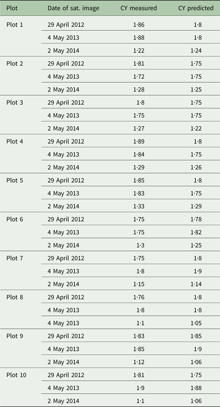
Table 10 shows the number of satellite images used for evaluation in the study and the number of plots used in the area. Different plots than those of the study area were also used to infer the real and estimated values of durum wheat production for 2012, 2013 and 2014 as shown in Table 11.
Crop yield data for t-test analysis

Crop yield (CY) real and predicted values for each plot

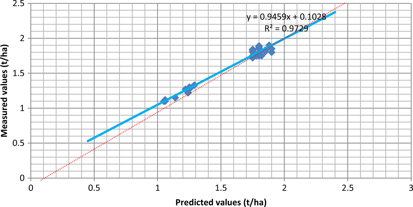
The results are shown graphically in Fig. 8, which indicates that the predicted and measured values of durum wheat are highly correlated. The plotted values in Fig. 8 between measured (Y-axis) and predicted (X-axis) values indicate that the developed model provides very good results for the test period. The linear trend of the values (blue colour) follows the diagonal (red dots) in the same direction and is also close to it, proving the developed model's accuracy.
Predicted v. measured yield values.

Furthermore, Table 12 illustrates that the developed algorithm can predict the production or yield in the field successfully under the current meteorological, soil and morphological conditions of the area. The t value given from the statistical analysis (t observed) was found to be smaller than the t value given from statistical tables or books (t statistical), which implies that, for n−1 degrees of freedom and at a confidence level of 95%, the predicted yield was not significantly different from the real yield (if t observed < t statistical then Ho:  $\sigma _1^2 = \sigma _2^2 $, where
 $\sigma _1^2 $ is the variation in crop yield measured and is the variation in crop yield predicted).
t-test results (obs.) compared with the statistical values (t stat.) of the test, for yield

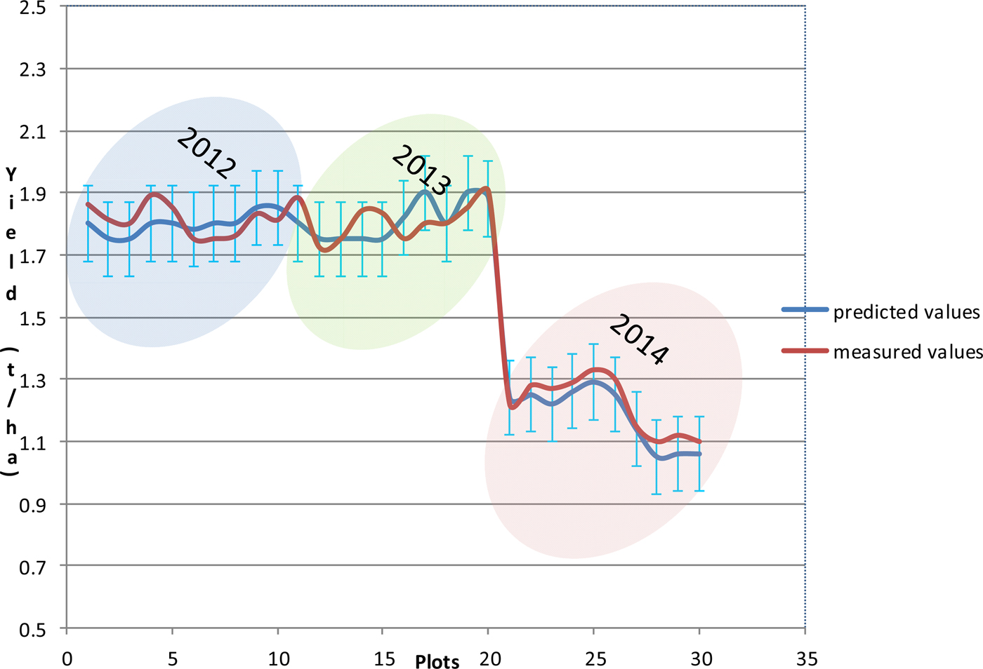
Figure 9 presents the results of the developed model application in practice. The s.e. of the model developed earlier also appears in the figure. The blue line represents the predicted values with the s.e. of the model (0·12) while the red line represents the values of the measured or real yield from the ten plots for the years 2012, 2013 and 2014. It is obvious that the measured values are within the deviation of the s.e. ranges for all the cases. Of vital importance for the specific semi-empirical model is that it also has the ability to work in drought conditions, as can be inferred from Fig. 9. The Department of Cyprus Meteorology refers to 2014 as a drought year, since the precipitation reached only 257 mm/year (September 2013 to September 2014), while for 2012 and 2013 the precipitation was 452 mm/year and 391 mm/year respectively for the study area. This implies that the model has a statistical consistency and can be applied under different conditions.
Measured and predicted (with s.e.) values of yield for 2012, 2013 and 2014.

Discussion
Based on the above examples provided for this purpose (groundnut, selected for the ETc and durum wheat, selected for the crop yield estimation) it can be concluded that:
If grey water values are taken for granted, there is the possibility of developing a specific model for estimating directly from satellite images not just the ETa but the value of water footprint. This can be done by applying an algorithm of the energy balance equilibrium for estimating evapotranspiration of each crop and simultaneously applying a crop yield estimation model in order to get the required (total) water per unit of production (yield).
The existing literature supports the use of SEBAL as the most promising algorithm that requires minimum input data of ground-based variables; it has been widely applied in several countries due to its accurate estimation of ETa. However, further research is required to apply such an algorithm and assess its effectiveness in different geographical areas with different meteorological and soil conditions. Indeed, application of the SEBAL algorithm in Cyprus, as performed in the present study, has shown that the algorithm could provide better results if fed with local empirical equations regarding crop canopy factors. It is the first time that the specific algorithm has been employed for estimating ETa in Cyprus. The modified SEBAL algorithm, named CYSEBAL, has been found to yield results close to the reference Epan method. This is an important finding, since it stresses the need to apply SEBAL taking into consideration local soil, geomorphological and meteorological conditions. The results of the t-test revealed that CYSEBAL was not significantly different from the Epan method and that the former can be used for estimating ETa in a systematic way. On the one hand, in its classic form, SEBAL could create anomalies in terms of irrigation planning, if it is not supported by appropriate empirical equations regarding crop canopy factors. On the other hand, CYSEBAL utilizes empirical equations and produces better results, especially at times when SEBAL deviates greatly from the Epan measurements. The hypothesis that the SEBAL algorithm could work better if supported with ground data was verified.
The present study also explored the potential of using remotely sensed measurements for obtaining accurate estimates of evapotranspiration, which can in turn provide irrigation managers and farmers with information that was not previously available and that can enhance irrigation performance for sustainable management of limited water resources.
With its semi-arid climatic characteristics, Cyprus is characterized by long-lasting very good weather conditions (>180 days of cloud-free days in a year) that allow the use of satellite remote sensing on a systematic basis. Despite the fact that Landsat-5 TM is an old sensor and Landsat-7 ETM+ faces several acquisition problems, Landsat covers the area of Cyprus twice every month and is still considered as one of the most useful tools for determining evapotranspiration. Future research consists of further applying the modified SEBAL algorithm using ASTER or SENTINEL 2 and examining more empirical relationships regarding crop canopy parameters of other crops too. Further research is required to include better resolution satellite imagery (most probably Sentinel 2), to improve the accuracy of the models or algorithms used and, to improve the results of the projected water footprint volumes. Higher accuracy translates to better water management efficiency.
The crop production environment consists of many crop and meteorological parameters that can affect production. The algorithm discussed in the present paper reasonably minimizes inconsistency and errors in yield prediction, giving high R 2 values, and was also found to provide yield values with no statistically significant difference from real values. The model takes into account the most basic parameters, which can be measured not only directly but also indirectly using remote sensing techniques. This enables potential users of the algorithm to use only remotely sensed data, once they have been correlated to the specific parameters. This was one of the main reasons for choosing the specific parameters. This method refers to prediction for durum wheat but can also be applied to other crops with the development of a similar semi-empirical model, after having the necessary parameter data which can be inferred only from satellite images if they are parameterized to vegetation indices of satellite imagery. Based on data obtained before harvest, crop yield can be predicted with acceptable accuracy. The model developed in the present work shows a promising result, which can be useful for supporting policy makers and producer's groups for developing sound agricultural policies based on scientific data.
Acknowledgements
Authors are grateful to the Agricultural Research Institute of Cyprus for providing scientific assistance and data during the project.