1 Introduction
The study of turbulent flows subjected to imposed periodic oscillations is closely related to both industrial applications (such as air flows in internal combustion engines and turbomachines, wakes of bluff bodies and acoustic wave propagation in in-duct systems) and biological fluid mechanics (such as blood flows in arteries). Depending on the mean flow, the oscillating flow can be classified as pulsatile (non-zero mean flow) or reciprocating (zero mean flow). Turbulent pulsatile flow is the subject to be discussed in this paper.
In a turbulent pulsatile flow field, the flow quantity
 $F(\boldsymbol{x},t)$
can be represented by the following triple decomposition, which was first introduced by Hussain & Reynolds (Reference Hussain and Reynolds1970):
 $$\begin{eqnarray}F(\boldsymbol{x},t)=\overline{F}(\boldsymbol{x})+\widetilde{F}(\boldsymbol{x},t)+F^{\prime }(\boldsymbol{x},t),\end{eqnarray}$$
where
 $\overline{F}$
is the time-averaged mean flow field,
 $\widetilde{F}$
is the perturbation field that is coherent with the imposed oscillation and
 $F^{\prime }$
corresponds to the turbulent fluctuations. The imposed oscillations can be seen as a time-varying forcing which breaks the equilibrium of the turbulent flow, and the perturbation field
 $\widetilde{F}$
, e.g. the velocity
 $\widetilde{u}_{i}$
or the Reynolds stress
 $\widetilde{u_{i}^{\prime }u_{j}^{\prime }}$
, is the response to the forcing. The determination of
 $\widetilde{F}$
in the turbulent boundary layer by theoretical models is the main objective of the present study, which is assisted by direct numerical simulation (DNS) for detailed inspection of the turbulent flow.
The present study is an extension of a previous investigation of sound propagation in low-Mach-number turbulent in-duct flows (Weng, Boij & Hanifi Reference Weng, Boij and Hanifi2013), where the objective was to understand the increase of the sound attenuation due to turbulence at low frequencies. Experiments have shown that the sound attenuation increases drastically when the frequency of the sound wave
 ${\it\omega}^{+}$
, normalized by the wall units of the turbulent boundary layer, is much smaller than 0.01 (Ronneberger Reference Ronneberger1975; Ronneberger & Ahrens Reference Ronneberger and Ahrens1977; Peters et al.
Reference Peters, Hirschberg, Reijnen and Wijnands1993; Allam & Åbom Reference Allam and Åbom2006). The increase of the attenuation can be attributed to the turbulent absorption effects in the boundary layer (Howe Reference Howe1995), i.e. the turbulence extracts the acoustic energy from the periodic straining of the sound wave and distributes the energy among structures with various time and length scales during the turbulent energy cascade. Such energy extraction and distribution become irreversible when the characteristic time of the cascade is much smaller than the sound wave period; therefore, the sound attenuation due to turbulent absorption is stronger at low frequencies. At high frequencies, on the other hand, the turbulent absorption becomes negligible due to the ‘fast’ cyclic straining of the sound wave compared with the energy cascade. In such high-frequency cases the flow state is ‘quasi-laminar’ for the sound wave since the flow affects the wave propagation only through its mean velocity profile. The above analysis indicates that the sound attenuation should be larger than its quasi-laminar value at low frequencies when the turbulent absorption is significant. However, a striking phenomenon takes place in an intermediate frequency range
 $0.006\lesssim {\it\omega}^{+}\lesssim 0.04,$
where the attenuation becomes even smaller than the quasi-laminar value, and reaches a local minimum at
 ${\it\omega}^{+}\approx 0.01$
. This phenomenon implies a reduction of the attenuation caused by the turbulence, and the reason is not completely understood yet.
Compared with the sound attenuation, a more general quantity to characterize the turbulent effects on the periodic oscillations is the dimensionless wall shear stress (scaled with its laminar Stokes value) of the perturbation field. The sound attenuation is physically related to the perturbation wall shear stress (Ronneberger & Ahrens Reference Ronneberger and Ahrens1977), while the shear stress is independent of the compressibility of the flow. Thus, the turbulent absorption effects, including the ‘striking phenomenon’, are also associated with the perturbation wall shear stress in incompressible pulsatile internal flows, i.e. the amplitude of the stress scaled by its laminar value is larger than unity at low frequencies, smaller than unity in the intermediate frequency range
 $0.006\lesssim {\it\omega}^{+}\lesssim 0.04$
and converges to unity at higher frequencies (Ronneberger & Ahrens Reference Ronneberger and Ahrens1977; Mao & Hanratty Reference Mao and Hanratty1986; Tardu & Binder Reference Tardu and Binder1993; Tardu, Binder & Blackwelder Reference Tardu, Binder and Blackwelder1994). Although the aforementioned energy extraction and distribution process qualitatively describes the behaviour of the perturbation field in the turbulent boundary layer, a quantitative description is difficult to provide due to the lack of detailed theoretical understanding of the turbulent boundary layer. Therefore, the turbulence–perturbation interaction has drawn attention through theoretical, experimental and computational efforts for more than five decades, from both the fluid mechanics and the acoustics community.
Modelling of the perturbation field in the turbulent boundary layer has been carried out since the 1960s. The most pioneering exploration is probably the one of Reynolds & Hussain (Reference Reynolds and Hussain1972), who first applied the triple decomposition in the Navier–Stokes equations to derive the perturbation equations, and realized that an accurate modelling for the perturbation Reynolds stress
 $\widetilde{u_{i}^{\prime }u_{j}^{\prime }}$
in the perturbation momentum equations is the key to describing the perturbation field.
Most models from the literature for the perturbation Reynolds stress are based on extending the standard eddy-viscosity model (EVM) in such a way that the effect of the Reynolds stress is treated as diffusion of the perturbation momentum. Usually, a dynamic quasi-static (or quasi-steady quasi-equilibrium) state between the imposed oscillation and the perturbation Reynolds stress is assumed and then the perturbation Reynolds stress tensor is directly linked to the perturbation strain tensor via a static eddy viscosity. Such quasi-static models in general fail to describe the perturbation quantities (e.g. the wall shear stress) accurately, especially in the intermediate and higher frequency ranges (Scotti & Piomelli Reference Scotti and Piomelli2002; Tardu & Costa Reference Tardu and Costa2005; Comte et al. Reference Comte, Haberkorn, Bouchet, Pagneux, Aurégan, Lamballais, Friedrich, Geurts and Métais2006; Weng et al. Reference Weng, Boij and Hanifi2013).
The failure of the quasi-static models is mainly due to the exclusion of the non-equilibrium effects, which are associated with the turbulence–perturbation interaction. Being similar to the aforementioned energy extraction and distribution process, the coherent oscillation in the Reynolds stress is caused by the periodic straining of the perturbation field. At low frequencies when the oscillation period is much larger than the turbulent relaxation time, the Reynolds stress responds to the straining almost instantly and a dynamic equilibrium (i.e. the quasi-static state) can be reached. At high frequencies, the equilibrium breaks down due to the ‘fast’ straining compared with the relaxation time, and a phase lag exists between the responding stress and the imposed straining, i.e. a non-equilibrium state is reached. The standard EVM forces the stress and strain tensors to be in phase, hence it becomes much less accurate at higher frequencies when the non-equilibrium effects are significant (Revell et al. Reference Revell, Benhamadouche, Craft and Laurence2006; Hamlington & Dahm Reference Hamlington and Dahm2008, Reference Hamlington and Dahm2009).
The non-equilibrium effects have been taken into account by several authors in both direct (Howe Reference Howe1995; Revell et al. Reference Revell, Benhamadouche, Craft and Laurence2006; Hamlington & Dahm Reference Hamlington and Dahm2008) and indirect (Ronneberger & Ahrens Reference Ronneberger and Ahrens1977; Mao & Hanratty Reference Mao and Hanratty1986; Mankbadi & Liu Reference Mankbadi and Liu1992; Brereton & Mankbadi Reference Brereton and Mankbadi1993; Peters et al. Reference Peters, Hirschberg, Reijnen and Wijnands1993) ways. Recently, the present authors proposed a linear non-equilibrium model (NEM) for the perturbation Reynolds stress, which can successfully predict the sound attenuation in the intermediate frequency range (Weng et al. Reference Weng, Boij and Hanifi2013). The proposed model assumes a constant turbulent relaxation time scale which allows one to conveniently include the non-equilibrium in the EVM in the frequency domain. The model can be further validated if the details of the perturbation field in the boundary layer are known. Compared with physical experiments where boundary layer measurements are rather difficult, the numerical simulation is a favourable means for the validation.
Direct numerical simulations/large eddy simulations (LES) have been performed for oscillating channel flows (Scotti & Piomelli Reference Scotti and Piomelli2001; Comte et al.
Reference Comte, Haberkorn, Bouchet, Pagneux, Aurégan, Lamballais, Friedrich, Geurts and Métais2006) and pipe flows (Manna, Vacca & Verzicco Reference Manna, Vacca and Verzicco2012, Reference Manna, Vacca and Verzicco2015), and they provide valuable insight into the perturbation field in the turbulent boundary layer. However, the oscillation amplitudes
 $a_{\mathit{cl}}$
(ratio of the perturbation to the mean bulk velocity) in these simulations are relatively large for validation purposes (
 $a_{\mathit{cl}}=0.7$
in Scotti & Piomelli (Reference Scotti and Piomelli2001), 0.2 in Comte et al. (Reference Comte, Haberkorn, Bouchet, Pagneux, Aurégan, Lamballais, Friedrich, Geurts and Métais2006) and larger than 1 in Manna et al. (Reference Manna, Vacca and Verzicco2015)), which may challenge the linearization assumption in the proposed NEM. The onset of nonlinear effects is inevitable during the production and transportation of the Reynolds stress
 $\widetilde{u_{i}^{\prime }u_{j}^{\prime }}$
, and it results in higher harmonic components in
 $\widetilde{u_{i}^{\prime }u_{j}^{\prime }}$
other than its fundamental mode at the forcing frequency. It is, however, worth examining the possibility of minimizing such effects by imposing oscillations with small amplitudes. In addition, the oscillation amplitudes may have effects on the statistics of the mean flow, while the mean flow in the NEM is assumed to be uninfluenced by the imposed oscillation. It is found from the literature that conclusions on the oscillation amplitude effect are somehow controversial, as some authors claim that such an effect is negligible (Mao & Hanratty Reference Mao and Hanratty1986; Brereton, Reynolds & Jayaraman Reference Brereton, Reynolds and Jayaraman1990; Tardu et al.
Reference Tardu, Binder and Blackwelder1994; Binder, Tardu & Vezin Reference Binder, Tardu and Vezin1995), while some, on the other hand, show the existence of such an effect even when
 $a_{\mathit{cl}}<1$
(current-dominated flow) (Ramaprian & Tu Reference Ramaprian and Tu1983; Tu & Ramaprian Reference Tu and Ramaprian1983).
Based on the aforementioned reasons, we choose to perform DNS for a fully developed pulsatile channel flow with a smaller oscillation amplitude,
 $a_{\mathit{cl}}=0.1$
. Both the nonlinear effect and the mean flow statistics are examined for this amplitude. Six forcing frequencies are chosen to cover the low, high and intermediate frequency ranges. The Reynolds number for the mean flow is
 $Re_{{\it\tau}}=350$
, which is chosen to be the same as in Scotti & Piomelli (Reference Scotti and Piomelli2001) and Comte et al. (Reference Comte, Haberkorn, Bouchet, Pagneux, Aurégan, Lamballais, Friedrich, Geurts and Métais2006) for convenience of comparison. The numerical results in the present study serve two purposes. One is to verify the behaviour of the perturbation field predicted by the NEM, and possibly to improve the model. The other is to expand the DNS/LES database in terms of the parameter space (
 $a_{\mathit{cl}}$
), and to provide data for the further validation of different models.
The paper is organized as follows. In § 2 the basic equations of motion for the pulsatile channel flow are introduced. In § 3 the set-up and results of the DNS are presented and discussed. In § 4 the non-equilibrium model is briefly reviewed. Validation and improvement of the reviewed model are presented. In § 5 some concluding remarks and outlook are given.
2 Equations of motion for pulsatile channel flow
Here, the motion of pulsatile turbulent channel flows is studied through numerical simulations of the Navier–Stokes equations
 $$\begin{eqnarray}\frac{\partial u_{i}}{\partial t}+u_{j}\frac{\partial u_{i}}{\partial x_{j}}=-\frac{\partial p}{\partial x_{i}}+\frac{1}{Re_{\mathit{cl}}}\,\frac{\partial ^{2}u_{i}}{\partial x_{j}\partial x_{j}}\end{eqnarray}$$
and
 $$\begin{eqnarray}\frac{\partial u_{i}}{\partial x_{i}}=0.\end{eqnarray}$$
A sketch of the channel geometry and the coordinate system used here is shown in figure 1, where
 $x$
,
 $y$
and
 $z$
denote the streamwise, wall-normal and spanwise directions respectively. Here, the three components of the velocity field
 $u_{i}$
in the
 $x$
,
 $y$
and
 $z$
directions are denoted by
 $u$
,
 $v$
and
 $w$
respectively. The Reynolds number in (2.1) is defined as
 $Re_{\mathit{cl}}=U_{\mathit{cl}}^{\ast }H^{\ast }/{\it\nu}^{\ast }$
, where
 $U_{\mathit{cl}}^{\ast }$
the centreline velocity of the laminar flow with the same flow rate as the turbulent mean flow,
 $H^{\ast }$
is the channel half-width and
 ${\it\nu}^{\ast }$
is the kinetic viscosity. Here, the asterisk denotes dimensional quantities.
Coordinate systems and sketch of the channel geometry. Here, the asterisk denotes dimensional quantities.

The equation for the mean flow field can be obtained by taking the time average of (2.1) and (2.2), which for the fully developed turbulent channel flow yields
 $$\begin{eqnarray}0=-\frac{\partial \overline{p}}{\partial x}+\frac{1}{Re_{\mathit{cl}}}\frac{\partial ^{2}\overline{u}}{\partial y^{2}}-\frac{\partial \overline{u^{\prime }v^{\prime }}}{\partial y},\end{eqnarray}$$
where
 $\overline{u^{\prime }v^{\prime }}$
is the mean Reynolds stress. In the modelling part of this work,
 $\overline{u^{\prime }v^{\prime }}$
is determined by the EVM, i.e.
 $$\begin{eqnarray}\overline{u^{\prime }v^{\prime }}=-\frac{{\it\nu}_{T}}{Re_{\mathit{cl}}}\,\frac{\partial \overline{u}}{\partial y},\end{eqnarray}$$
where
 ${\it\nu}_{T}$
is the eddy viscosity. Here, we focus on situations where the amplitude of the perturbation is small enough to meet the linearization requirement; thus, the equation for the mean flow quantities, including the eddy viscosity
 ${\it\nu}_{T}$
, is assumed to be unchanged compared with the case without pulsations (Reynolds & Hussain Reference Reynolds and Hussain1972).
If the imposed oscillation forcing is homogeneous in the streamwise and spanwise directions, and a harmonic oscillation is assumed, i.e.
 $\widetilde{F}(\boldsymbol{x},t)=\text{Re}[\hat{F}(\boldsymbol{x})\exp (\text{i}{\it\omega}t)]$
, with
 ${\it\omega}$
being the angular frequency of the perturbation, then the equation for the perturbation field reads (Mao & Hanratty Reference Mao and Hanratty1986)
 $$\begin{eqnarray}\text{i}{\it\omega}\widetilde{u}=-\frac{\partial \widetilde{p}}{\partial x}+\frac{1}{Re_{\mathit{cl}}}\,\frac{\partial ^{2}\widetilde{u}}{\partial y^{2}}-\frac{\partial \widetilde{r}}{\partial y},\end{eqnarray}$$
where the time derivative
 $\partial /\partial t$
is replaced by
 $\text{i}{\it\omega}$
. Equation (2.5) corresponds to the linearized perturbation equations proposed by Reynolds & Hussain (Reference Reynolds and Hussain1972) when the advection is neglected.
The perturbation Reynolds stress term
 $\widetilde{r}$
in (2.5) is defined as
 $$\begin{eqnarray}\widetilde{r}=\langle u^{\prime }v^{\prime }\rangle -\overline{u^{\prime }v^{\prime }},\end{eqnarray}$$
which is the oscillation of the background Reynolds stress due to the imposed pulsations. Here,
 $\langle \cdot \rangle$
denotes the phase average of quantities. For flow fields that are statistically homogeneous in both the streamwise and the spanwise directions the phase average can be defined as
 $$\begin{eqnarray}\langle F(y,t)\rangle =\lim _{N_{p}\rightarrow \infty }\frac{1}{N_{p}L_{z}L_{x}}\mathop{\sum }_{n=0}^{N_{p}}\int _{0}^{L_{z}}\int _{0}^{L_{x}}F\left(\boldsymbol{x},t+\frac{2{\rm\pi}n}{{\it\omega}}\right)\text{d}x\,\text{d}z,\quad 0\leqslant t\leqslant \frac{2{\rm\pi}}{{\it\omega}},\end{eqnarray}$$
where
 $N_{p}$
is the total number of periods in the recorded time history. Equation (2.5) is a URANS (unsteady Reynolds-averaged Navier–Stokes)-like modelling for the pulsatile flow in the frequency domain. In order to solve the equation, the perturbation Reynolds stress term
 $\widetilde{r}$
must be modelled. In the simplest case one may assume that the oscillating Reynolds stress has no influence on the dynamics of the perturbation field, i.e.
 $\widetilde{r}$
can be discarded from (2.5) and the flow becomes ‘quasi-laminar’. In this case the Stokes boundary layer equation is recovered.
For channel flow, where the Stokes layer should be symmetric about the channel centreline (i.e.
 $\partial \widetilde{u}/\partial y=0$
for
 $y=1$
), an analytical solution to (2.5) can be derived:
 $$\begin{eqnarray}\widetilde{u}=\frac{\text{i}}{{\it\omega}}\frac{\partial \widetilde{p}}{\partial x}\left[1-\frac{1}{1+\exp (2\mathscr{K})}\exp (\mathscr{K}y)-\frac{\exp (2\mathscr{K})}{1+\exp (2\mathscr{K})}\exp (-\mathscr{K}y)\right],\end{eqnarray}$$
where
 $\mathscr{K}=\sqrt{\text{i}{\it\omega}Re_{\mathit{cl }}}$
. If one further assumes that the thickness of the Stokes layer is much smaller than the channel half-width
 $H$
, the Stokes layer given by (2.8) recovers to the well-known flat-plate Stokes solution
 $$\begin{eqnarray}\widetilde{u}_{\mathit{s}}=\widetilde{u}_{\mathit{s,cl}}\left[1-\exp (-\mathscr{K}y)\right]=\widetilde{u}_{\mathit{s,cl}}\left\{1-\exp \left[\left(-{\it\alpha}_{\mathit{s}}-\text{i}\frac{2{\rm\pi}}{{\it\lambda}_{\mathit{s}}}\right)y\right]\right\}.\end{eqnarray}$$
Here,
 $\widetilde{u}_{\mathit{s,cl}}=\text{i}{\it\omega}^{-1}\partial \widetilde{p}/\partial x=|\widetilde{u}_{\mathit{s,cl}}|\exp (\text{i}{\it\omega}t+\text{i}{\it\Phi}_{\widetilde{u}_{\mathit{cl}},\mathit{s}})$
is the channel centreline velocity with phase
 ${\it\Phi}_{\widetilde{u}_{\mathit{cl}},\mathit{s}}$
. Moreover,
 ${\it\alpha}_{\mathit{s}}=1/l_{s}$
and
 ${\it\lambda}_{\mathit{s}}=2{\rm\pi}l_{s}$
are the damping coefficient and the wavelength respectively of the shear wave component
 $\widetilde{u}_{\mathit{s,cl}}\exp [(-{\it\alpha}_{\mathit{s}}-\text{i}2{\rm\pi}/{\it\lambda}_{\mathit{s}})y]$
, and
 $l_{s}=\sqrt{2}({\it\omega}Re_{\mathit{cl}})^{-1/2}$
is the Stokes layer thickness. The subscript ‘
 $s$
’ indicates the ‘Stokes solution’ and the subscript ‘
 $cl$
’ indicates the ‘centreline value’.
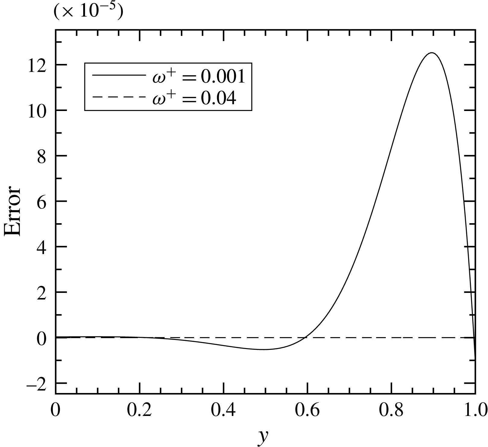
It should be noted that the flat-plate Stokes solution (2.9) may differ from (2.8) at low frequencies when the Stokes layer thickness is comparable with the channel width. The difference is, however, negligible for the frequency range of interest in this paper, as can be seen in figure 2. We therefore use the Stokes solution as the quasi-laminar solution in the rest of the paper, since it has been conventionally used for channel flow.


The perturbation wall shear stress
 $\widetilde{{\it\tau}}_{\mathit{w,s}}$
can then be computed from the Stokes solution as
 $$\begin{eqnarray}\widetilde{{\it\tau}}_{\mathit{w,s}}=\frac{1}{Re_{\mathit{cl}}}\left.\frac{\partial \widetilde{u}_{\mathit{s}}}{\partial y}\right|_{y=0}=A_{\widetilde{{\it\tau}},s}\exp (\text{i}{\it\omega}t+\text{i}{\it\Phi}_{\widetilde{{\it\tau}},s}),\end{eqnarray}$$
where
 $$\begin{eqnarray}A_{\widetilde{{\it\tau}},s}=\frac{\sqrt{2}}{Re_{\mathit{cl}}}{\it\alpha}_{\mathit{s}}\left|\widetilde{u}_{\mathit{s,cl}}\right|\quad \text{ and }\quad {\it\Phi}_{\widetilde{{\it\tau}},s}={\it\Phi}_{\widetilde{u}_{\mathit{cl}},s}+{\rm\pi}/4\end{eqnarray}$$
are the amplitude and phase of the oscillating wall shear stress respectively. Equation (2.11) shows that in the Stokes solution the phase lead of the wall shear stress to the centreline velocity is
 ${\rm\pi}/4$
.
Previous studies (Ronneberger & Ahrens Reference Ronneberger and Ahrens1977; Mao & Hanratty Reference Mao and Hanratty1986; Tardu et al.
Reference Tardu, Binder and Blackwelder1994; Scotti & Piomelli Reference Scotti and Piomelli2001) have shown that the Stokes solution (2.10) is valid for the perturbation field in a turbulent flow if the frequency of the imposed oscillation is high enough so that the boundary layer of the perturbation field stays essentially within the turbulent viscous sublayer. In this case, mixing of momentum by the turbulent eddies is hardly experienced by the perturbation field. At lower pulsation frequencies, on the other hand, the perturbation boundary layer extrudes into the region where turbulent mixing is effective; the wall shear stress therefore deviates from the Stokes solution (2.10). The turbulent diffusion can be taken into account by introducing a proper model for
 $\widetilde{r}$
in (2.5). Some of the existing models are discussed in § 4.
3 Direct numerical simulation
Direct numerical simulations are performed for a pulsatile flow with
 $Re_{{\it\tau}}=u_{{\it\tau}}^{\ast }H^{\ast }/{\it\nu}^{\ast }=350$
, corresponding to
 $Re=U_{b}^{\ast }H^{\ast }/{\it\nu}^{\ast }\approx 6052$
, or
 $Re_{\mathit{cl}}=U_{\mathit{cl}}^{\ast }H^{\ast }/{\it\nu}^{\ast }\approx 9000$
based on the centreline velocity of the laminar flow, where
 $u_{{\it\tau}}^{\ast }$
is the mean wall friction velocity and
 $U_{b}^{\ast }$
is the bulk velocity of the turbulent mean flow.
3.1 Simulation set-up
Simulations are performed using the SIMSON code (Chevalier et al. Reference Chevalier, Schlatter, Lundbladh and Henningson2007), which solves the incompressible Navier–Stokes equations in the velocity–vorticity formulation. The solver uses Fourier expansions in the streamwise and spanwise directions, and Chebychev polynomials with Gauss–Lobatto grids in the wall-normal direction. Information about the grid resolution is given in table 1, where enhanced spatial resolution based on the DNS set-up by Scotti & Piomelli (Reference Scotti and Piomelli2001) is used to guarantee the numerical convergence. The boundary conditions in the horizontal directions are periodic, and at both of the non-permeable walls there are no-slip boundary conditions.
The grid resolution for
 $Re_{{\it\tau}}=350$
. The grid spacings
 ${\rm\Delta}x^{+}$
,
 ${\rm\Delta}y^{+}$
and
 ${\rm\Delta}z^{+}$
are normalized by the wall units;
 $N_{x}$
,
 $N_{y}$
and
 $N_{z}$
are the numbers of grids in the
 $x$
,
 $y$
and
 $z$
directions respectively.

The periodic pulsation is generated by enforcing a pressure gradient as
 $$\begin{eqnarray}\frac{\partial p}{\partial x}=-\left(\frac{Re_{{\it\tau}}}{Re_{\mathit{cl}}}\right)^{2}\left[1+{\it\beta}\,\cos \left(\frac{Re_{{\it\tau}}^{2}}{Re_{\mathit{cl}}}{\it\omega}_{f}^{+}t\right)\right],\end{eqnarray}$$
where
 ${\it\beta}$
is a parameter controlling the amplitude of the pulsating force and
 ${\it\omega}_{f}^{+}$
denotes the forcing frequency. To characterize the amplitude of the imposed pulsation, the ratio of the perturbation velocity amplitude to the mean velocity at the channel centreline, i.e.
 $a_{\mathit{cl}}=|\widetilde{u}_{\mathit{cl}}^{\ast }|/U_{\mathit{cl}}^{\ast }=|\widetilde{u}_{\mathit{cl}}|$
, is conventionally used. The relation between
 $a_{\mathit{cl}}$
and
 ${\it\beta}$
can be determined from (2.5) and (3.1), yielding
 $$\begin{eqnarray}a_{\mathit{cl}}=\frac{{\it\beta}}{{\it\omega}_{f}^{+}Re_{\mathit{cl}}},\end{eqnarray}$$
where the fact that the total perturbation stresses vanish at the channel centreline is used. The value of
 $a_{\mathit{cl}}$
in this study is
 $0.1$
, which is the smallest so far compared with previous simulations (Scotti & Piomelli Reference Scotti and Piomelli2001; Comte et al.
Reference Comte, Haberkorn, Bouchet, Pagneux, Aurégan, Lamballais, Friedrich, Geurts and Métais2006) for similar physical problems. Six cases with different forcing frequencies are used; see table 2. The frequencies are chosen to possibly reach the quasi-static state and the intermediate state respectively. For the convenience of the reader, the corresponding Stokes lengths
 $l_{\mathit{s}}^{+}$
are also given in table 2.
The forcing frequencies
 ${\it\omega}_{f}^{+}$
, and their corresponding Stokes lengths
 $l_{\mathit{s}}^{+}$
, used in the DNS.

The flow is initialized by setting
 ${\it\beta}=0$
, and is regarded as fully developed when the time-averaged friction velocity
 $u_{{\it\tau}}$
on both of the walls satisfies
 $u_{{\it\tau}}=\sqrt{-\partial \overline{p}/\partial x}=Re_{{\it\tau}}/Re_{\mathit{cl}}$
. Then, the periodic forcing is added with a given frequency, and the friction velocity starts to transitionally oscillate around values that deviate from
 $Re_{{\it\tau}}/Re_{\mathit{cl}}$
. The data acquisition starts after the flow is stabilized, i.e. when the friction velocity oscillates around
 $Re_{{\it\tau}}/Re_{\mathit{cl}}$
.
3.2 Data evaluation and statistics
The acquired data are reduced by phase and time averages. Here, the phase-averaging, defined in (2.7), is performed by dividing the period into 32 bins of equal width, and the desired velocities
 $\langle u_{i}\rangle$
and Reynolds stresses
 $\langle u_{i}^{\prime }u_{j}^{\prime }\rangle$
are averaged in each bin. It should be mentioned that the phase-averaged Reynolds stresses in this study are obtained by
 $$\begin{eqnarray}\langle u_{i}^{\prime }u_{j}^{\prime }\rangle =\langle u_{i}u_{j}\rangle -\langle u_{i}\rangle \langle u_{j}\rangle\end{eqnarray}$$
in order to skip obtaining the turbulent fluctuation velocity
 $u_{i}^{\prime }$
separately.
The time average is performed by taking the mean of the phase-averaged data within one period. Since the derived phase-averaged data can be written as
 $\langle u_{i}\rangle =\overline{u}_{i}+\widetilde{u}_{i}$
and
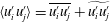 $\langle u_{i}^{\prime }u_{j}^{\prime }\rangle =\overline{u_{i}^{\prime }u_{j}^{\prime }}+\widetilde{u_{i}^{\prime }u_{j}^{\prime }}$
, the perturbation quantities can then be obtained by subtracting the mean quantities from the phase-averaged ones.
For the given amplitudes and frequencies of the perturbations,
 $\langle u_{i}\rangle$
generally converges after approximately 100 integrations, while
 $\langle u_{i}^{\prime }u_{j}^{\prime }\rangle$
requires more integrations. A reference value for the required integration time is the one used by Tardu et al. (Reference Tardu, Binder and Blackwelder1994) for the experiment, which is
 $10^{5}Re_{\mathit{cl}}/Re_{{\it\tau}}^{2}$
. However, this value for the current DNS set-up is approximately 7000, which is unrealistic in terms of computational cost. In this study we regard
 $\langle u_{i}^{\prime }u_{j}^{\prime }\rangle$
as being converged when its amplitude is symmetric about
 $y=1$
, i.e. the channel centreline; in this way the required integration time becomes much lower than 7000 for all of the frequency cases.
It should be noticed that neither
 $\widetilde{u}_{i}$
nor
 $\widetilde{u_{i}^{\prime }u_{j}^{\prime }}$
is necessarily a pure sine function, i.e. they contain higher harmonic components other than the fundamental mode in their Fourier spectra. This is due to the nonlinear effects during the production and transportation process of
 $\widetilde{u_{i}^{\prime }u_{j}^{\prime }}$
, which spread the energy at the forcing frequency to other frequency components. Despite the use of a small forcing amplitude in the DNS to suppress nonlinear effects, the onset of such effects is inevitable, and this would definitely affect the validation of the linear NEM by using the DNS data. In § 3.4.2 the harmonic components in
 $\widetilde{u}_{i}$
and
 $\widetilde{u_{i}^{\prime }u_{j}^{\prime }}$
will be examined in order to evaluate the level of the nonlinearity.
3.3 The mean flow field and the turbulence structures
In order to examine the sensitivity of the mean flow field to the imposed oscillation, the DNS results corresponding to a steady case (flow without pulsations) and an unsteady one (pulsating flow with
 ${\it\omega}_{f}^{+}=0.04$
) are analysed. The mean velocity
 $\overline{u}^{+}$
and the stress tensor components
 $\overline{u_{i}^{\prime }u_{j}^{\prime }}^{+}$
are shown in figures 3 and 4 respectively. The results are also compared with earlier published data, which for the pulsating channel flow come from the DNS of Scotti & Piomelli (Reference Scotti and Piomelli2001) with
 $Re_{{\it\tau}}=350$
and
 ${\it\omega}_{f}^{+}=0.04$
, and for the steady channel flow the DNS of Moser, Kim & Mansour (Reference Moser, Kim and Mansour1999) with
 $Re_{{\it\tau}}=395$
. We also present the mean flow profile computed using an algebraic EVM based on the
 ${\it\nu}_{T}$
proposed by She et al. (Reference She, Wu, Chen and Hussain2012) (see appendix A). To validate the algebraic EVM, the mean velocity profile is computed from (2.3) and (A 1), by setting
 $\partial \overline{p}/\partial x=-(Re_{{\it\tau}}/Re_{\mathit{cl}})^{2}$
. The obtained profile is plotted in figure 3. It can be seen that the algebraic model fits well to our DNS data. This EVM is used later for the evaluation of our models.
Mean velocity profiles in flows with and without pulsations.

Figure 3 shows that the mean velocity profiles from the DNS for both the steady and the unsteady flows agree well with the DNS results from Moser et al. (Reference Moser, Kim and Mansour1999), both in the viscous sublayer and in the log-law region, with a maximum difference of
 ${\approx}2\,\%$
. In comparison, the DNS data of Scotti & Piomelli (Reference Scotti and Piomelli2001) with
 $a_{\mathit{cl}}\approx 0.7$
give larger values in the log-law region. This indicates that the mean velocity is barely influenced by the pulsation when the pulsation amplitude is small, such as
 $a_{\mathit{cl}}=0.1$
in the current DNS, but could be modified by pulsations with larger amplitudes, such as
 $a_{\mathit{cl}}\approx 0.7$
in Scotti & Piomelli (Reference Scotti and Piomelli2001).
Similar conclusions can also be drawn when comparing the Reynolds stress tensors, as shown in figure 4. It should be noted that the distribution of
 $\overline{u_{i}^{\prime }u_{j}^{\prime }}^{+}$
against
 $y^{+}$
depends on the Reynolds number, so the data of Moser et al. (Reference Moser, Kim and Mansour1999) with
 $Re_{{\it\tau}}=395$
in figure 4 can merely be treated as reference values. However, the DNS of Scotti & Piomelli (Reference Scotti and Piomelli2001) is for the same Reynolds number as ours. It displays a decrease of the turbulent kinetic energy and the Reynolds stress magnitude compared with our DNS data for the steady flow, being at maximum 13 %, 23 %, 33 % and 23 % smaller for
 $\overline{u^{\prime }u^{\prime }}^{+}$
,
 $\overline{v^{\prime }v^{\prime }}^{+}$
,
 $\overline{w^{\prime }w^{\prime }}^{+}$
and
 $-\overline{u^{\prime }v^{\prime }}^{+}$
respectively. These differences may also be attributed to the larger pulsation amplitude in their simulation. In comparison, our DNS of unsteady flow in figure 4 again confirms that the mean flow is barely influenced by the small-amplitude pulsation. Besides the amplitude
 $a_{\mathit{cl}}$
, figure 5 shows that the mean flow statistics are also insensitive to the chosen frequencies, confirming the assumption of the mean flow in the present study being uninfluenced by the pulsation. As a consequence, the eddy viscosity
 ${\it\nu}_{T}$
can be calculated from steady mean flow models.
Time-averaged stress tensor components.

Mean velocity profiles (
 $a$
) and stress tensor components (
 $b$
) calculated from the DNS data of the current study with the six oscillating frequencies (see table 2). The figure shows that the mean flow statistics are insensitive to the imposed oscillation with the chosen pulsation amplitude and frequencies.

Besides the mean flow statistics, the topology of the turbulent structures might also be changed by the imposed oscillations. For example, Scotti & Piomelli (Reference Scotti and Piomelli2001) and Comte et al. (Reference Comte, Haberkorn, Bouchet, Pagneux, Aurégan, Lamballais, Friedrich, Geurts and Métais2006) have shown that, when the pulsation amplitude is large enough (
 $a_{\mathit{cl}}\approx 0.7$
in their simulations), relaminarization can take place, and the acceleration and deceleration phases are not symmetric within one oscillation cycle. For the current DNS with
 $a_{\mathit{cl}}=0.1$
, however, relaminarization is not observed. This is demonstrated in figure 6, where the streamwise turbulent fluctuation velocity
 $u^{\prime }$
is displayed for the case of
 ${\it\omega}_{f}^{+}=0.02$
. The figure shows that the flow is in a fully turbulent regime throughout the cycle, and the pattern of the streak structures is not influenced by the imposed oscillations. This again confirms the validity of using steady mean flow turbulence models to calculate the eddy viscosity
 ${\it\nu}_{T}$
.
Contours of the streamwise turbulent fluctuation velocity
 $u^{\prime }$
in the
 $y^{+}=10.5$
plane, with
 ${\it\omega}_{f}^{+}=0.02$
. Two contours are used between
 $-0.8$
and
 $0.376$
, with the most positive values in grey and the most negative values in black. The phase within the cycle,
 $t/T_{f}$
, is defined based on the imposed forcing in (3.1). Here,
 $T_{f}$
is the forcing period and (a)
 $t/T_{f}=0/8$
, (b)
 $t/T_{f}=1/8$
, (c)
 $t/T_{f}=2/8$
, (d)
 $t/T_{f}=3/8$
, (e)
 $t/T_{f}=4/8$
, (f)
 $t/T_{f}=5/8$
, (g)
 $t/T_{f}=6/8$
, (h)
 $t/T_{f}=7/8$
.

The time evolution of
 $(a)$
the centreline perturbation velocity
 $\widetilde{u}_{\mathit{cl}}$
and
 $(b)$
the perturbation wall stress
 $\widetilde{{\it\tau}}_{\mathit{w}}$
. The phase within the cycle,
 $t/T_{f}$
, is defined based on the imposed forcing in (3.1). Here,
 $T_{f}$
is the forcing period. The grey region in the figure is the deceleration phase when
 $-\partial \widetilde{p}/\partial x<0$
, while the other region is the acceleration phase when
 $-\partial \widetilde{p}/\partial x>0$
.

3.4 The perturbation field
In this subsection, the DNS results for the perturbation field are presented. First, the time evolution of the perturbation field is shown. Then, Fourier analysis is applied to the results to inspect the dominant modes in detail.
3.4.1 Time evolution of the perturbation field
Using the data reduction techniques introduced in § 3.2, we can derive the perturbation velocities and Reynolds stresses as
 $$\begin{eqnarray}\widetilde{u}_{i}=\langle u_{i}\rangle -\overline{u}_{i}\quad \text{and}\quad \widetilde{u_{i}^{\prime }u_{j}^{\prime }}=\langle u_{i}^{\prime }u_{j}^{\prime }\rangle -\overline{u_{i}^{\prime }u_{j}^{\prime }}\end{eqnarray}$$
respectively. The time evolutions of these perturbation quantities are shown in figures 7 and 8 to inspect the physical aspects of the flow.
The time evolution of the perturbation Reynolds stresses at different phases of the wave cycle for different forcing frequencies: (a,f,k,p)
 ${\it\omega}_{f}^{+}=0.001$
, (b,g,l,q)
 ${\it\omega}_{f}^{+}=0.006$
, (c,h,m,r)
 ${\it\omega}_{f}^{+}=0.01$
, (d,i,n,s)
 ${\it\omega}_{f}^{+}=0.02$
, (e,j,o,t)
 ${\it\omega}_{f}^{+}=0.04$
. The profiles are
 $T_{f}/32$
apart, and are offset by
 $1\times 10^{-4}$
,
 $8\times 10^{-4}$
,
 $1.2\times 10^{-4}$
and
 $2\times 10^{-4}$
units in the vertical direction for
 $\widetilde{r}$
,
 $\widetilde{u^{\prime }u^{\prime }}$
,
 $\widetilde{v^{\prime }v^{\prime }}$
and
 $\widetilde{w^{\prime }w^{\prime }}$
respectively. The dashed lines mark the positions of the Stokes lengths
 $l_{\mathit{s}}^{+}$
, whose values are listed in table 2.

Figure 7 shows the time evolution of the centreline perturbation velocity
 $\widetilde{u}_{\mathit{cl}}$
and the perturbation wall stress
 $\widetilde{{\it\tau}}_{\mathit{w}}$
, defined by
 $$\begin{eqnarray}\widetilde{{\it\tau}}_{\mathit{w}}=\frac{1}{Re_{\mathit{cl}}}\left.\frac{\partial \widetilde{u}}{\partial y}\right|_{y=0}.\end{eqnarray}$$
For the cases with
 ${\it\omega}_{f}^{+}\leqslant 0.003$
, figure 7(a) shows that the perturbation velocities at the channel centreline oscillate with magnitudes larger than the expected value
 $a_{\mathit{cl}}=0.1$
. This is due to the intrusion of the shear waves into the channel centre, which may lead to strong couplings of the inner and outer layers (Scotti & Piomelli Reference Scotti and Piomelli2001). Such intrusion is absent at higher forcing frequencies, e.g.
 ${\it\omega}_{f}^{+}\geqslant 0.006$
, when the inner and outer layers are only weakly coupled. Therefore, at high frequencies the perturbation velocities oscillate with the expected magnitude
 $a_{\mathit{cl}}=0.1$
. The
 $45^{\circ }$
phase lag between
 $\widetilde{u}_{\mathit{cl}}$
and
 $\widetilde{{\it\tau}}_{\mathit{w}}$
is also observed for the highest forcing frequency
 ${\it\omega}_{f}^{+}=0.04$
, indicating that the shear wave behaves as it does in laminar flows, so the Stokes solution given by (2.10) and (2.11) is recovered. The phase lag is smaller in the lower-frequency cases.
From the above results, we see that the response of the turbulence to the imposed oscillations exhibits a frequency dependence. Such a dependence can also be observed by looking at the time evolutions of the shear and normal perturbation Reynolds stresses, which are plotted in figure 8. The figures reveal two main characteristics of the perturbation fields. First, the Reynolds stress amplitudes show a decreasing trend as the frequency increases. The reason is that when the forcing frequency is low the turbulence has ample time to respond to the ‘slow’ oscillations. Therefore, energies can be effectively extracted from the perturbation fields and be transported among Reynolds stress components. When the forcing frequency is high, the turbulence has less time to react to the oscillations within a cycle. The response of the turbulence therefore seems to be ‘frozen’, resulting in small amplitudes of the perturbation Reynolds stresses. The second characteristic of the perturbation fields is derived by observing the oscillation patterns of the Reynolds stresses. At high frequencies (
 ${\it\omega}_{f}^{+}\geqslant 0.02$
), the peaks of the Reynolds stresses propagate from where they are generated (near the reference Stokes layer edge
 $l_{\mathit{s}}^{+}$
) towards the channel centre. A complete wavelength can be clearly observed. At lower frequencies (
 ${\it\omega}_{f}^{+}=0.006$
and 0.01), the propagation behaviour is still observable for
 $\widetilde{r}$
,
 $\widetilde{v^{\prime }v^{\prime }}$
and
 $\widetilde{w^{\prime }w^{\prime }}$
, the peaks of which, however, travel a distance shorter than one wavelength when they reach the channel centre. For the stress
 $\widetilde{u^{\prime }u^{\prime }}$
, the propagation behaviour is less observable compared with the other three stresses. The propagation component in
 $\widetilde{u^{\prime }u^{\prime }}$
seems to be submerged by another component, one that oscillates at
 $y^{+}\approx 10$
without propagating. In the lowest-frequency case (
 ${\it\omega}_{f}^{+}=0.001$
), the propagation behaviour is indiscernible for all of the Reynolds stresses; the non-propagating component seems to dominate through the whole cycle.
The time evolution of the production terms
 $\mathscr{P}_{I}$
,
 $\mathscr{P}_{II}$
,
 $\mathscr{P}_{IV}$
and
 $\mathscr{P}_{V}$
at different phases of the wave cycle for different forcing frequencies: (a,f)
 ${\it\omega}_{f}^{+}=0.001$
, (b,g)
 ${\it\omega}_{f}^{+}=0.006$
, (c,h)
 ${\it\omega}_{f}^{+}=0.01$
, (d,i)
 ${\it\omega}_{f}^{+}=0.02$
, (e,j)
 ${\it\omega}_{f}^{+}=0.04$
. See (3.6) and (3.7) for the definition of the production. The profiles are
 $T_{f}/4$
apart, and are offset by
 $1\times 10^{-3}$
units for
 $\mathscr{P}_{I}$
and
 $\mathscr{P}_{II}$
, and by
 $2\times 10^{-3}$
units for
 $\mathscr{P}_{IV}$
and
 $\mathscr{P}_{V}$
, in the vertical direction:
 $\frac{\qquad }{}$
,
 $\mathscr{P}_{I}$
and
 $\mathscr{P}_{IV}$
; —
 $+$
—,
 $\mathscr{P}_{II}$
and
 $\mathscr{P}_{V}$
. The dashed lines mark the positions of the Stokes lengths
 $l_{\mathit{s}}^{+}$
, whose values are listed in table 2.

The two characteristics described above can be further analysed by inspecting the energy production of the stresses. The equations of the perturbation Reynolds stresses read
 $$\begin{eqnarray}\frac{\partial \widetilde{r}}{\partial t}=\underbrace{-\overline{v^{\prime }v^{\prime }}\frac{\partial \widetilde{u}}{\partial y}}_{\mathscr{P}_{I}}\underbrace{-\widetilde{v^{\prime }v^{\prime }}\frac{\partial \overline{u}}{\partial y}}_{\mathscr{P}_{II}}\underbrace{-\widetilde{v^{\prime }v^{\prime }}\frac{\partial \widetilde{u}}{\partial y}}_{\mathscr{P}_{III}}+\cdots\end{eqnarray}$$
and
 $$\begin{eqnarray}\frac{\partial \widetilde{u^{\prime }u^{\prime }}}{\partial t}=\underbrace{-\overline{u^{\prime }v^{\prime }}\frac{\partial \widetilde{u}}{\partial y}}_{\mathscr{P}_{IV}}\underbrace{-\widetilde{r}\frac{\partial \overline{u}}{\partial y}}_{\mathscr{P}_{V}}\underbrace{-\widetilde{r}\frac{\partial \widetilde{u}}{\partial y}}_{\mathscr{P}_{VI}}+\cdots \,.\end{eqnarray}$$
In figure 9 the time evolutions of the linear production terms
 $\mathscr{P}_{I}$
,
 $\mathscr{P}_{II}$
,
 $\mathscr{P}_{IV}$
and
 $\mathscr{P}_{V}$
within one cycle are shown. It should be noted that the transportation and dissipation terms are not shown in (3.6) and (3.7). It should also be noted that the productions of
 $\widetilde{v^{\prime }v^{\prime }}$
and
 $\widetilde{w^{\prime }w^{\prime }}$
are identically zero.
The production process may be described as follows. At the early stage of each cycle, the mean stresses first extract energy from the perturbation straining through
 $\mathscr{P}_{I}$
and
 $\mathscr{P}_{IV}$
. Then, the generated
 $\widetilde{r}$
participates in the productions
 $\mathscr{P}_{V}$
and
 $\mathscr{P}_{VI}$
instantly, while the generated
 $\widetilde{u^{\prime }u^{\prime }}$
would first redistribute its energy to
 $\widetilde{v^{\prime }v^{\prime }}$
through the pressure transport and then
 $\widetilde{v^{\prime }v^{\prime }}$
participates in the productions
 $\mathscr{P}_{II}$
and
 $\mathscr{P}_{III}$
.
As has been discussed above while describing the first Reynolds stress characteristic, the energy redistributed from
 $\widetilde{u^{\prime }u^{\prime }}$
to
 $\widetilde{v^{\prime }v^{\prime }}$
is of larger amount at low frequencies than at high frequencies. Therefore, the production term
 $\mathscr{P}_{II}$
, which is oscillated by the stress
 $\widetilde{v^{\prime }v^{\prime }}$
, has larger amplitude at lower frequencies. This in turn results in larger amplitudes of
 $\widetilde{r}$
and
 $\widetilde{u^{\prime }u^{\prime }}$
at low frequencies. Such low-frequency efficiency of the energy redistribution among perturbation Reynolds stresses is proved in figure 9, where the amplitudes of
 $\mathscr{P}_{II}$
and
 $\mathscr{P}_{V}$
display a decreasing trend as the frequency increases. The low-frequency efficiency serves as an explanation for the first characteristic of the perturbation fields.
The second characteristic of the perturbation Reynolds stresses, i.e. the propagation behaviour of the peaks of the stresses at low and high frequencies, could also trace its origin from
 $\mathscr{P}_{I}$
,
 $\mathscr{P}_{II}$
,
 $\mathscr{P}_{IV}$
and
 $\mathscr{P}_{V}$
. We can look at the terms
 $\mathscr{P}_{I}$
and
 $\mathscr{P}_{IV}$
, and identify that the oscillating part, i.e. the perturbation shear strain rate
 $\partial \widetilde{u}/\partial y$
, in these two terms inherently exhibits propagation behaviour due to the shear wave component in
 $\widetilde{u}$
. At high frequencies, the thickness of the perturbation boundary layer is small (as indicated by the Stokes layer thickness
 $l_{\mathit{s}}^{+}$
in figure 9), so the propagation of the shear wave can be clearly observed between the boundary layer and the channel centre. This results in the manifested propagation behaviour of
 $\mathscr{P}_{I}$
and
 $\mathscr{P}_{IV}$
in the high-frequency cases (
 ${\it\omega}_{f}^{+}\geqslant 0.02$
) in figure 9. At lower frequencies, the perturbation boundary layer is thicker, so the shear wave propagates a shorter distance before it reaches the channel centre. This leads to the less noticeable propagation behaviour of
 $\mathscr{P}_{I}$
and
 $\mathscr{P}_{IV}$
in the low-frequency cases (
 ${\it\omega}_{f}^{+}\leqslant 0.01$
), as shown in figure 9. Because the perturbation Reynolds stresses are produced by
 $\mathscr{P}_{I}$
and
 $\mathscr{P}_{IV}$
in a direct or an indirect manner, the second characteristic of the Reynolds stresses is therefore explained by the oscillation patterns of
 $\mathscr{P}_{I}$
and
 $\mathscr{P}_{IV}$
.
Compared with
 $\mathscr{P}_{I}$
and
 $\mathscr{P}_{IV}$
, which are shear-strain-oscillated productions (SSOPs), the other two production terms
 $\mathscr{P}_{II}$
and
 $\mathscr{P}_{V}$
are Reynolds-stress-oscillated productions (RSOPs). The RSOPs show oscillation patterns similar to those of the SSOPs, and they together with the SSOPs determine the second characteristic of the perturbation Reynolds stresses. The dominant role between the RSOPs and the SSOPs in the production process varies with the frequency, as shown in figure 9. At low frequencies, the RSOPs dominate over the SSOPs in the production of the Reynolds stresses; therefore, the produced Reynolds stresses show strong correlations to the RSOPs. For example, the abovementioned non-propagating feature of
 $\widetilde{u^{\prime }u^{\prime }}$
at
 ${\it\omega}_{f}^{+}=0.001$
is more similar to the oscillation pattern of the RSOP,
 $\mathscr{P}_{V}$
(see figure 9), than that of the SSOP,
 $\mathscr{P}_{IV}$
. At higher frequencies, the amplitudes of the RSOPs and the SSOPs are comparable; therefore, the net production depends on the phase difference between the RSOPs and the SSOPs, i.e. whether it is destructive or constructive interference between the RSOPs and the SSOPs.
The above analysis regarding the energy production only involves the linear terms,
 $\mathscr{P}_{I}$
,
 $\mathscr{P}_{II}$
,
 $\mathscr{P}_{IV}$
and
 $\mathscr{P}_{V}$
, which are the major contributions in the production process. In comparison, the nonlinear terms,
 $\mathscr{P}_{III}$
and
 $\mathscr{P}_{VI}$
, have minor contributions to the productions; they do, however, participate in the redistribution of energies among different frequency components. In the next section the fundamental and harmonic frequency components are shown and discussed.
3.4.2 Fundamental and harmonic components in the perturbation field
As has been mentioned at the end of §§ 3.4.1 and 3.2, both
 $\widetilde{u}_{i}$
and
 $\widetilde{u_{i}^{\prime }u_{j}^{\prime }}$
contain harmonic components in their Fourier spectra caused by nonlinear effects. In this subsection Fourier analysis is applied to the DNS results to inspect the spectrum of the perturbation field. The level of the nonlinearity is also discussed.
The Fourier component amplitudes of the perturbation field at
 $y^{+}=87.5$
, obtained by applying fast Fourier transform (FFT) to the DNS data. The forcing frequency is
 ${\it\omega}_{f}^{+}=0.01$
. (a) The amplitude of the perturbation velocity
 $|\widetilde{u}|$
and (b) the amplitude of the perturbation Reynolds stress
 $|\widetilde{r}|$
.

The fundamental and first harmonic mode shapes of (
 $a$
) the perturbation velocity
 $|\widetilde{u}|$
and (
 $b$
) the perturbation Reynolds stress
 $|\widetilde{r}|$
, obtained from FFT of the DNS data. The forcing frequency is
 ${\it\omega}_{f}^{+}=0.01$
. In (
 $a$
) the solutions to the linear perturbation equation (2.5) are also shown, where the Reynolds stress
 $\widetilde{r}$
is taken from the DNS data as shown in (
 $b$
).
The Fourier spectra of
 $\widetilde{u}$
and
 $\widetilde{r}$
obtained from the DNS data for
 ${\it\omega}_{f}^{+}=0.01$
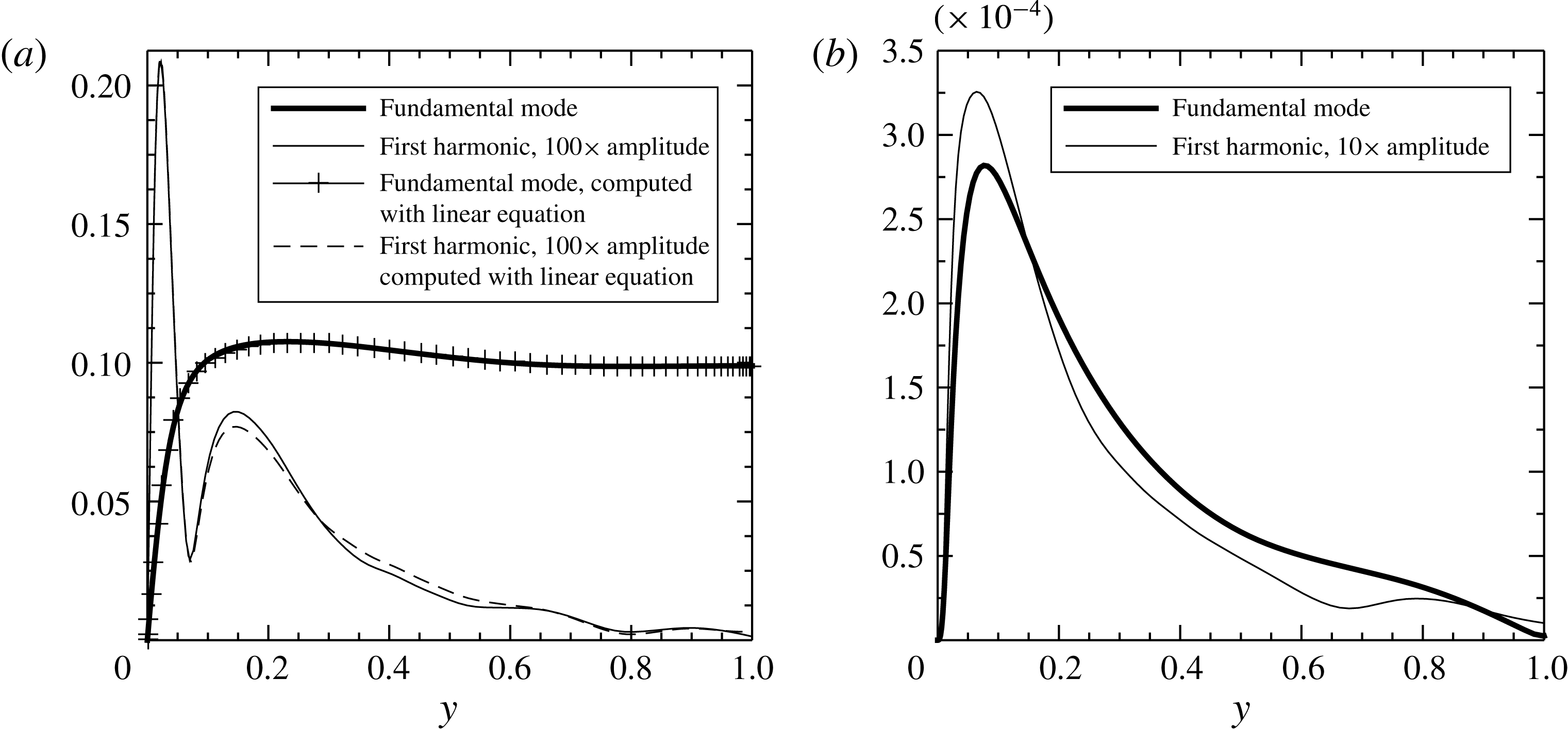
are plotted in figure 10. The graphs clearly show the existence of the harmonic components in addition to the fundamental modes, and the first harmonic in general dominates over the other higher harmonics. To inspect the details of the modes, the mode shapes of the fundamental and its first harmonic for
 $\widetilde{u}$
and
 $\widetilde{r}$
are shown in figure 11. These plots correspond to
 ${\it\omega}_{f}^{+}=0.01$
. The graphs show that, while the fundamental mode shape of
 $\widetilde{u}$
looks similar to the Stokes solution, the first harmonic component of
 $\widetilde{u}$
displays a very different mode shape. On the other hand, the fundamental and the first harmonic of
 $\widetilde{r}$
display similarities in their mode shapes. It should be noted that the nonlinear interactions generating the harmonics only take place in the production and transport of
 $\widetilde{r}$
, but not in the transport of
 $\widetilde{u}$
. This can be shown by looking at the incompressible perturbation equation (2.5), where the transport by the perturbation
 $\widetilde{u}_{j}\partial \widetilde{u}_{i}/\partial x_{j}$
is zero due to the streamwise and spanwise homogeneity. Then, the only source for the higher harmonics in
 $\widetilde{u}$
is the Reynolds stress
 $\widetilde{r}$
. This is verified by using the Reynolds stresses shown in figure 11(
 $b$
) as the forces in (2.5) to compute the fundamental and the first harmonic of
 $\widetilde{u}$
. It should be noted that
 $\partial \widetilde{p}/\partial x$
in (2.5) is absent when computing the harmonic components. The computed results, shown in figure 11(
 $a$
), agree well with the DNS data in both shape and amplitude.
The fundamental mode shapes of the perturbation shear and normal stresses versus
 $y^{+}$
: (a)
 $|\tilde{r}^{+}|$
, (b)
 $|\widetilde{u^{\prime }u^{\prime }}^{+}|$
, (c)
 $|\widetilde{v^{\prime }v^{\prime }}^{+}|$
, (d)
 $|\widetilde{w^{\prime }w^{\prime }}^{+}|$
. It is shown that the maxima of the stresses decrease with increase of the frequency, except for the normal stress
 $\widetilde{u^{\prime }u^{\prime }}^{+}$
.

The first harmonic mode shapes of the perturbation shear and normal stresses versus
 $y^{+}$
: (a)
 $|\tilde{r}^{+}|$
, (b)
 $|\widetilde{u^{\prime }u^{\prime }}^{+}|$
, (c)
 $|\widetilde{v^{\prime }v^{\prime }}^{+}|$
, (d)
 $|\widetilde{w^{\prime }w^{\prime }}^{+}|$
.

The level of the nonlinearity
 ${\it\Pi}$
, defined by (3.8), at the six forcing frequencies (see table 2 for the
 ${\it\omega}_{f}^{+}$
). The symbols represent the value of
 ${\it\Pi}$
for: ▫,
 $\widetilde{r}$
; ○,
 $\widetilde{u^{\prime }u^{\prime }}$
;
 $\diamondsuit$
,
 $\widetilde{v^{\prime }v^{\prime }}$
;
 $\unicode[STIX]{x204E}$
,
 $\widetilde{w^{\prime }w^{\prime }}$
.

The fundamental and first harmonic mode shapes of
 $\widetilde{u_{i}^{\prime }u_{j}^{\prime }}$
are presented in figures 12 and 13 respectively. There, one can observe different frequency dependences of the fundamental mode and its first harmonic. The peak amplitude of the fundamental mode decreases monotonically on increasing the forcing frequency. The exception is the normal stress
 $\widetilde{u^{\prime }u^{\prime }}^{+}$
, which shows a small increment at
 ${\it\omega}_{f}^{+}=0.006$
and 0.01. For the first harmonic mode, the peak amplitudes of the Reynolds stresses in figure 13 increase with the frequency when
 ${\it\omega}_{f}^{+}\leqslant 0.006$
, and decrease with the frequency when
 ${\it\omega}_{f}^{+}>0.006$
.
Now, we evaluate the level of nonlinearity by comparing the amplitudes of the harmonic modes with the fundamental one. In figure 10, it can be seen that the first harmonic mode in general is the most dominant among the higher harmonics. Therefore, we only use the first harmonic mode and compare it with the fundamental one in order to evaluate the level of nonlinearity. We define it as the ratio of the peak amplitude of the first harmonic mode to that of the fundamental mode, i.e.
 $$\begin{eqnarray}{\it\Pi}=\max (|\widetilde{u_{i}^{\prime }u_{j}^{\prime }}|_{2{\it\omega}_{f}^{+}})/\max (|\widetilde{u_{i}^{\prime }u_{j}^{\prime }}|_{{\it\omega}_{f}^{+}}).\end{eqnarray}$$
It can be seen from figure 14 that the overall nonlinearity level is less than
 $0.17$
, indicating that the nonlinear terms in the perturbation Reynolds stress equations play a minor role compared with the linear terms. This justifies the use of linear models to compute the main features of the perturbation fields.
The characteristic of the first harmonic mode has a direct impact on the nonlinearity level
 ${\it\Pi}$
. The values of
 ${\it\Pi}$
for all four Reynolds stresses reach a maximum for an intermediate value of frequency,
 ${\it\omega}_{f}^{+}=0.006$
. This indicates that the energy redistribution towards higher harmonics is most efficient at this frequency compared with the other five frequencies. It is interesting to note that a significant increase of the nonlinear effects occurs in the intermediate frequency range, where the ‘striking phenomenon’ of sound attenuation also occurs (see § 1).
4 Modelling of the perturbation Reynolds stress
 $\widetilde{r}$

In this section, the linear NEM, together with the quasi-static model, is reviewed and compared with the DNS results.
4.1 Review of the existing models
For the modelling of the perturbation Reynolds stress
 $\widetilde{r}$
, almost all previous studies (Reynolds & Hussain Reference Reynolds and Hussain1972; Ronneberger & Ahrens Reference Ronneberger and Ahrens1977; Howe Reference Howe1984; Mao & Hanratty Reference Mao and Hanratty1986; Mankbadi & Liu Reference Mankbadi and Liu1992; Scotti & Piomelli Reference Scotti and Piomelli2002) have assumed the existence of an eddy viscosity for the perturbation field. The eddy viscosity for a simple shear flow such as the case studied in this paper can be derived by using the Prandtl mixing length theory from Ronneberger & Ahrens (Reference Ronneberger and Ahrens1977), Howe (Reference Howe1984) and Pope (Reference Pope2000):
 $$\begin{eqnarray}\langle u^{\prime }v^{\prime }\rangle =-l_{\mathit{m}}^{2}\left[\frac{\partial (\overline{u}+\widetilde{u})}{\partial y}\right]^{2},\end{eqnarray}$$
where
 $l_{\mathit{m}}$
is the mixing length, which is assumed not to be modulated by the imposed oscillation. Combining (2.4) and (4.1), and neglecting the nonlinear term of
 $\widetilde{u}$
, we obtain the first-order approximation for
 $\widetilde{r}$
:
 $$\begin{eqnarray}\widetilde{r}=-\frac{2{\it\nu}_{T}}{Re_{\mathit{cl}}}\frac{\partial \widetilde{u}}{\partial y}.\end{eqnarray}$$
It should be noticed that the EVM discussed above prescribes that the (negative) Reynolds stress
 $\widetilde{r}$
and the shear strain rate
 $\partial \widetilde{u}/\partial y$
be in phase. However, studies (Revell et al.
Reference Revell, Benhamadouche, Craft and Laurence2006; Yu & Girimaji Reference Yu and Girimaji2006; Hamlington & Dahm Reference Hamlington and Dahm2008, Reference Hamlington and Dahm2009) of turbulent flows subject to unsteady shear have shown that a phase lag between the Reynolds stress and the mean strain rate exists. This lag is due to the non-equilibrium effects (or the memory effects (Builtjes Reference Builtjes1977)) associated with the unsteadiness. Such non-equilibrium effects are absent in (4.2) due to the lack of the phase lag, and thus (4.2) represents a modelling of the perturbation Reynolds stress in a quasi-equilibrium, or quasi-static, limit.
One way to attempt to include the non-equilibrium effects in the modelling is to relax the perturbation Reynolds stress
 $\widetilde{r}$
, which can be represented by the following relaxation equation:
 $$\begin{eqnarray}\frac{\partial \widetilde{r}}{\partial t}=-\frac{1}{t_{T}}\widetilde{r}-\frac{2{\it\nu}_{T}}{t_{T}Re_{\mathit{cl}}}\frac{\partial \widetilde{u}}{\partial y},\end{eqnarray}$$
where
 $t_{T}$
is a turbulent relaxation time scale of the turbulent flow. Equation (4.3) was originally derived from the basic dynamic equations for the Reynolds stress tensor
 $u_{i}^{\prime }u_{j}^{\prime }$
, with a linearization similar to that proposed by Hamlington & Dahm (Reference Hamlington and Dahm2008). In addition, the diffusive transport of
 $\widetilde{r}$
is assumed to be unmodulated by the pulsation. A more elaborate derivation of (4.3) can be found in Weng et al. (Reference Weng, Boij and Hanifi2013). A rough estimation of the time scale
 $t_{T}$
in the turbulent boundary layer was originally suggested by Ronneberger (Reference Ronneberger1991) (as cited in Peters et al. (Reference Peters, Hirschberg, Reijnen and Wijnands1993)) to be of the order of
 $t_{T}=100Re_{\mathit{cl}}/Re_{{\it\tau}}^{2}$
. This value was later tuned through comparison with experimental data for sound attenuation in turbulent pipe flows (Weng Reference Weng2013; Weng et al.
Reference Weng, Boij and Hanifi2013), giving
 $$\begin{eqnarray}t_{T}=150\frac{Re_{\mathit{cl}}}{Re_{{\it\tau}}^{2}}.\end{eqnarray}$$
By using the turbulent time scale in (4.4), and assuming that the perturbation has a time dependence of
 $\exp (\text{i}{\it\omega}t)$
, we obtain the following solution to (4.3):
 $$\begin{eqnarray}\widetilde{r}=-W\frac{2{\it\nu}_{T}}{Re_{\mathit{cl}}}\frac{\partial \widetilde{u}}{\partial y},\end{eqnarray}$$
where
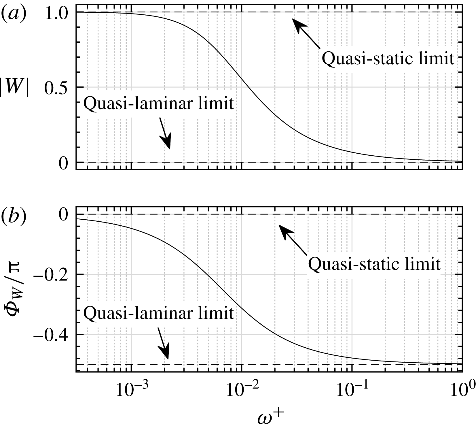
 $$\begin{eqnarray}W=\frac{1}{1+\text{i}{\it\omega}t_{T}}=\frac{1}{1+150\text{i}{\it\omega}^{+}}.\end{eqnarray}$$
In (4.6), the dimensionless angular frequency scaled by wall units,
 ${\it\omega}^{+}={\it\omega}Re_{\mathit{cl}}/Re_{{\it\tau}}^{2}={\it\omega}^{\ast }{\it\nu}^{\ast }/u_{{\it\tau}}^{\ast 2}$
, is used for convention and convenience purposes.
Equation (4.5) shows that the inclusion of the non-equilibrium state, i.e. the time dependence of the stress, brings a phase lag
 $-\!\arctan ({\it\omega}t_{T})=-\!\arctan (150{\it\omega}^{+})$
between the negative Reynolds stress and the strain rate. This phase lag vanishes as
 ${\it\omega}^{+}\rightarrow 0$
, i.e. when the quasi-static state is reached, and then the model given by (4.2) is recovered. As
 ${\it\omega}^{+}$
increases towards infinity, i.e. reaching a highly non-equilibrium state, the phase lag approaches
 $-{\rm\pi}/2$
. In the rest of the paper, the model given by (4.2) is referred to as the ‘quasi-static model’ (QSM), while the model given by (4.5) is referred to as the ‘non-equilibrium model’ (NEM), for convenience of reference.
Unlike the QSM, which treats the turbulent eddies as purely viscous, the NEM instead treats the eddies as viscoelastic. This can be seen from (4.3): the shear strain rate
 $\partial \widetilde{u}/\partial y$
consists of two parts, a ‘viscous’ contribution
 $-(Re_{\mathit{cl}}/2{\it\nu}_{T})\widetilde{r}$
and an ‘elastic’ contribution
 $-(Re_{\mathit{cl}}/{\it\varepsilon}_{T})(\partial \widetilde{r}/\partial t)$
, with
 ${\it\varepsilon}_{T}=2{\it\nu}_{T}/t_{T}$
as the ‘eddy elasticity’ being analogous to the elastic modulus in Maxwell’s viscoelastic model (Fung & Tong Reference Fung and Tong2001). Therefore, the introduced phase lag in the NEM can be interpreted as the consequence of the viscoelastic characteristics of the turbulent eddies. This viscoelastic property of the turbulence is consistent with the prediction by Crow (Reference Crow1968).
The real and imaginary parts of
 $W$
in (4.6), as functions of
 ${\it\omega}t_{T}$
and
 ${\it\omega}^{+}$
.

In the frequency domain, the inclusion of the elastic contribution of the eddies to the pulsatile flow is equivalent to bringing in a complex frequency dependence
 $W$
to the eddy viscosity, as indicated by (4.5) and (4.6), where the real and imaginary parts of the complex ‘eddy-viscosity’ term represent the viscous and elastic contributions respectively. The frequency characteristics of these two contributions are fully described by
 $W$
. Figure 15 shows the real and imaginary parts of
 $W$
as a function of the frequency. The graph indicates that at the quasi-static state (
 ${\it\omega}t_{T}\ll 1$
or
 ${\it\omega}^{+}\ll 1/150\approx 0.01$
), the viscous effects dominate. When
 ${\it\omega}t_{T}$
is approximately 1 or
 ${\it\omega}^{+}$
is approximately 0.01, these two effects are comparable and the elastic effect reaches a peak at
 ${\it\omega}t_{T}=1$
or
 ${\it\omega}^{+}=1/150$
; as the frequency increases, the elastic effect first dominates, and then both of the effects are negligible in the pulsatile flow at high frequencies, i.e. in the highly non-equilibrium state.
4.2 Comparison between the models and the DNS
4.2.1 The perturbation velocity
$\widetilde{u}$

The near-wall behaviour of the perturbation velocity
 $\widetilde{u}$
is usually characterized by the wall shear stress
 $\widetilde{{\it\tau}}_{\mathit{w}}$
, as defined by (3.5). If the momentum of the perturbation field is diffused by the molecular viscous forces only, then
 $\widetilde{{\it\tau}}_{\mathit{w}}$
should recover to the Stokes solution
 $\widetilde{{\it\tau}}_{\mathit{w,s}}$
, as given by (2.10). Otherwise, the deviation of
 $\widetilde{{\it\tau}}_{\mathit{w}}$
from
 $\widetilde{{\it\tau}}_{\mathit{w,s}}$
indicates extra diffusion effects due to the turbulent mixing. Whether such turbulent diffusion effects are significant for the perturbation field depends on the value of
 ${\it\omega}^{+}$
(or
 $l_{\mathit{s}}^{+}$
which is related to
 ${\it\omega}^{+}$
by
 $l_{\mathit{s}}^{+}=\sqrt{2/{\it\omega}^{+}}$
) (Ronneberger & Ahrens Reference Ronneberger and Ahrens1977). Figure 16 demonstrates the relation between
 $\widetilde{{\it\tau}}_{\mathit{w}}$
and
 ${\it\omega}^{+}$
, where the experimental data from Ronneberger & Ahrens (Reference Ronneberger and Ahrens1977) and Tardu et al. (Reference Tardu, Binder and Blackwelder1994), the LES data from Scotti & Piomelli (Reference Scotti and Piomelli2001) and the solutions computed from the QSM and the NEM are shown together with the DNS results. In addition, a linear model based on the rapid distortion theory (RTD) proposed by Brereton & Mankbadi (Reference Brereton and Mankbadi1993) is also used for comparison. Here, the amplitude of the wall shear stress
 $\widetilde{{\it\tau}}_{\mathit{w}}$
, denoted by
 $A_{\widetilde{{\it\tau}}}$
in the figure, is normalized by the Stokes solution
 $A_{\widetilde{{\it\tau}},s}$
, see (2.10), and the phase lead of the wall shear stress to the centreline perturbation velocity is shown in the figure.
The wall shear stress
 $\widetilde{{\it\tau}}_{\mathit{w}}$
. (a) Amplitude of the stress
 $A_{\widetilde{{\it\tau}}}$
normalized by the Stokes solution
 $A_{\widetilde{{\it\tau}},s}$
(see (2.10)). (b) Phase difference (in degrees) between the stress and the centreline perturbation velocity. The experimental data are taken from Ronneberger & Ahrens (Reference Ronneberger and Ahrens1977) (RA) and Tardu et al. (Reference Tardu, Binder and Blackwelder1994) (TA), and the LES data are taken from Scotti & Piomelli (Reference Scotti and Piomelli2001) (SP). The model based on RDT is the one proposed by Brereton & Mankbadi (Reference Brereton and Mankbadi1993). It should be noted that the Reynolds numbers of the experimental data are estimated from the measurement descriptions in the corresponding papers, and the values of
 $a_{\mathit{cl}}$
for RA are taken from Comte et al. (Reference Comte, Haberkorn, Bouchet, Pagneux, Aurégan, Lamballais, Friedrich, Geurts and Métais2006).

The DNS, LES and experimental data in figure 16 all show that the values of
 $A_{\widetilde{{\it\tau}}}/A_{\widetilde{{\it\tau}},s}$
and
 ${\it\Phi}_{\widetilde{{\it\tau}}}-{\it\Phi}_{\widetilde{u}_{\mathit{cl}}}$
asymptotically converge to the Stokes solution values of 1 and
 ${\rm\pi}/4$
(
 $45^{\circ }$
) respectively as the frequency increases. Such behaviour indicates that the turbulent diffusion effects are negligible for the perturbation field at high frequencies,
 ${\it\omega}^{+}\gtrsim 0.04$
. This high-frequency behaviour corresponds to the quasi-laminar state of the pulsating flow, since the turbulent Reynolds stresses are absent. When the frequency decreases from
 ${\it\omega}^{+}\approx 0.04$
, the onset of turbulent diffusion effects is observed as the values start to deviate from the Stokes solution.
One consequence of such effects is an increase of the wall shear stress amplitude from its quasi-laminar values, except for an intermediate frequency interval where the stress amplitude is smaller than that in the quasi-laminar state, and a minimum amplitude occurs at approximately
 ${\it\omega}^{+}=0.01$
. This near-wall behaviour of the perturbation field within this intermediate frequency interval is nearly independent of the pulsating amplitude
 $a_{\mathit{cl}}$
and the Reynolds number, as clearly shown by the DNS, LES and experimental data in figure 16. The scattering of the data of Tardu et al. (Reference Tardu, Binder and Blackwelder1994) is regarded as being due to the accuracy of the measurement; the data, however, also display minimum values around the same frequency, i.e.
 ${\it\omega}^{+}\approx 0.01$
.
To explain the behaviour of the perturbation field in this intermediate frequency range, a first step could be to aim for an accurate model of the perturbation Reynolds stress
 $\widetilde{r}$
in (2.5). The QSM (4.2) and the NEM (4.5) for
 $\widetilde{r}$
are discussed here. Figure 16(a) shows that the QSM is able to predict the turbulent diffusion effects on the perturbation field only at low and high frequencies; it, however, completely fails in the intermediate frequency range. On the other hand, the NEM has good performance in both the low and the intermediate frequency ranges, including the prediction of the minimum value of
 $A_{\widetilde{{\it\tau}}}/A_{\widetilde{{\it\tau}},s}$
. An analysis based on the NEM indicates that the behaviour of the perturbation field around the minimum value is due to the viscoelastic characteristics of the turbulent flow: the frequency-domain solution (4.5) relates the strain rate and the stress by a complex frequency-dependent ‘eddy viscosity’. As has been discussed in § 4.1, this complex ‘eddy viscosity’ recognizes the turbulent eddies as viscoelastic. It can be shown that the elastic contribution tends to increase the boundary layer thickness of the shear wave, and thence tends to decrease the wall friction. The negative peak of the elastic contribution occurs at approximately
 ${\it\omega}^{+}=0.01$
(see figure 15), where the minimum value of
 $A_{\widetilde{{\it\tau}}}/A_{\widetilde{{\it\tau}},s}$
is located. Therefore, the behaviour of the perturbation field in the intermediate frequency range can be attributed to the elastic contribution of the eddies.
It should be noticed that the RDT model also predicts the local minimum of
 $A_{\widetilde{{\it\tau}}}/A_{\widetilde{{\it\tau}},s}$
at
 ${\it\omega}^{+}\approx 0.01$
. The model, however, fails to predict the increase of the wall shear stress amplitude caused by the turbulent diffusion when
 ${\it\omega}^{+}\lesssim 0.005$
.
Regarding the phase lead in figure 16(b), the DNS, LES and experimental data show that the value of the phase lead decreases from the Stokes solution
 $45^{\circ }$
as
 ${\it\omega}^{+}$
decreases from 0.02. At lower frequencies (
 ${\it\omega}^{+}<0.006$
), the data obtained from different simulations and experiments start to deviate, and seem to be dependent on the Reynolds number. The scattering of the data can be interpreted as follows. At lower frequencies, the shear wave boundary layer becomes thicker and may intrude beyond the channel centre. Then the shear waves generated at the opposite sides of the channel wall interfere with each other. The distance between the shear wave boundary layer and the channel centreline can be estimated by the ratio
 $l_{\mathit{s}}^{+}/Re_{{\it\tau}}$
; the larger this ratio is, the easier it is for the shear wave to intrude into the channel centre. Thus, at a given low frequency, the shear wave behaviour becomes Reynolds-number-dependent. The question of how to determine the frequency above which the shear wave is independent of the Reynolds number is discussed in detail in § 4.4.
(a) The amplitude of the perturbation velocity
 $\widetilde{u}$
(normalized by its centreline value
 $\widetilde{u}_{\mathit{cl}}$
) and (b) the phase lead (rad) of
 $\widetilde{u}$
to its centreline value
 $\widetilde{u}_{\mathit{cl}}$
for the six forcing frequencies
 ${\it\omega}_{f}^{+}=0.001$
to
 $0.04$
: ○, DNS; ——, NEM; — ⋅ —, QSM; – – –, Stokes solution.

The amplitude of the perturbation velocity
 $\widetilde{u}$
(normalized by its centreline value
 $\widetilde{u}_{\mathit{cl}}$
) and the phase lead (rad) of
 $\widetilde{u}$
to its centreline value
 $\widetilde{u}_{\mathit{cl}}$
, zoomed into the outer layer for the three forcing frequencies
 ${\it\omega}_{f}^{+}=0.01$
(a,b), 0.02 (c,d), 0.04 (e,f): ○, DNS; ——, NEM; — ⋅ —, QSM; – – –, Stokes solution.

It can be seen from figure 16(b) that, compared with the QSM and the RDT, the NEM results computed with
 $Re_{{\it\tau}}=350$
show better agreement with the experimental and simulation data. However, the NEM displays oscillations that are not supported by the simulations or the experimental data in the range of
 $0.013\lesssim {\it\omega}^{+}\lesssim 0.04$
. These oscillations are caused by the inaccurate prediction of
 $\widetilde{u}$
in the outer layer, whose value at the channel centreline is used to compute the phase lead. To demonstrate the cause of this, the profiles of
 $\widetilde{u}$
computed from the NEM are compared with the DNS results in figure 17. Shown together with the NEM in the figure are the QSM and the Stokes solution.
First, we can look at the amplitude of the perturbation velocity
 $\widetilde{u}$
in figure 17. In general, the inner-layer performance of the NEM shows better agreement with the DNS than the other two models. In particular, the other two models overestimate the slope of
 $\widetilde{u}$
near the wall at intermediate frequencies,
 ${\it\omega}_{f}^{+}=0.01$
and
 $0.02$
. This is the reason why these two models do not predict the local minimum in the wall shear stress (see the plot of
 $A_{\widetilde{{\it\tau}}}/A_{\widetilde{{\it\tau}},s}$
in figure 16). In the outer layer, however, the performance of the NEM is not as good, especially at
 ${\it\omega}_{f}^{+}=0.01$
, 0.02 and 0.04, where the damping coefficient and the wavelength of the shear wave, as defined in (2.9), are significantly underestimated (see figure 18 for the velocity profiles zoomed into the outer layer). This is attributed to the use of a constant turbulent time scale
 $t_{T}$
in the NEM equation (4.5), as will be discussed in § 4.3. Even so, some features of the shear wave propagation in the turbulence are qualitatively revealed by the NEM: the DNS data show that the shear wave in the turbulent flow at
 ${\it\omega}^{+}=0.01$
, 0.02 and 0.04 exhibits extended propagation compared with the Stokes solution, which indicates a smaller damping coefficient experienced by the shear wave in a turbulent flow than in a laminar flow. Such extended propagation has also been observed by Hartmann (Reference Hartmann2001). The reason for the reduced damping coefficient, according to the NEM, is the elastic property of the eddies at the intermediate frequencies, which tends to decrease the damping coefficient of the shear wave compared with a purely viscous flow. However, the NEM is unable to predict the damping coefficient quantitatively.
Second, we can look at the relative phase of the perturbation velocity plotted in figure 17, which shows that no significant advantages of the NEM over the other two models are found. However, the reduced damping coefficient of the shear wave is observed in the phase profile as well, as shown by the DNS data in the cases of
 ${\it\omega}_{f}^{+}=0.01$
, 0.02 and 0.04, where the velocity displays extended propagation of the shear wave (see figure 18 for the velocity profiles zoomed into the outer layer). This extended, or less damped, shear wave propagation is again qualitatively described by the NEM, but the value of the damping coefficient is underestimated. Such underestimation may result in inaccurate prediction of the phase of
 $\widetilde{u}$
in the channel centreline at low Reynolds numbers, and this is the reason for the unphysical oscillation of the NEM result in figure 16(b), where the centreline phase of
 $\widetilde{u}$
is used to scale the wall shear stress. The influence of the inaccuracy would decrease as the Reynolds number increases, since at high enough Reynolds numbers the incorrectly predicted shear wave would die out before it reaches the channel centreline. To show this, the value of
 ${\it\Phi}_{\widetilde{{\it\tau}}}-{\it\Phi}_{\widetilde{u}_{\mathit{cl}}}$
computed by the NEM but with a Reynolds number much higher than 350 is shown in figure 16(b), and it is observed that the non-physical oscillation disappears.
4.2.2 The perturbation Reynolds stress
$\widetilde{r}$

To further examine the performance of the NEM, the perturbation Reynolds stress
 $\widetilde{r}$
obtained from the DNS is compared with the model.
According to the NEM, the amplitude of
 $\widetilde{r}$
decreases as the pulsating frequency increases from the quasi-static limit to a highly non-equilibrium state, and a phase lag appears between the perturbation stress and the strain rate. This can be seen clearly by writing
 $W$
in (4.6) as
 $W=|W|\text{e}^{\text{i}{\it\Phi}_{W}}$
, where
 $$\begin{eqnarray}\left.\begin{array}{@{}l@{}}|W|={\displaystyle \frac{1}{\sqrt{1+({\it\omega}t_{T})^{2}}}},\\ {\it\Phi}_{W}=-\!\arctan {\it\omega}t_{T}\end{array}\right\}\end{eqnarray}$$
are the amplitude and phase of
 $W$
respectively, and they are plotted in figure 19 by using the time scale in (4.4). The relation in (4.5) shows that the value of
 $|W|$
determines how the amplitude of
 $\widetilde{r}$
varies with the frequency for a given Reynolds number, and
 ${\it\Phi}_{W}$
indicates the phase lag between
 $-\widetilde{r}$
and the shear strain rate
 $\partial \widetilde{u}/\partial y$
, i.e.
 $$\begin{eqnarray}{\it\Phi}_{W}={\it\Phi}_{-\widetilde{r}}-{\it\Phi}_{\partial \widetilde{u}/\partial y},\end{eqnarray}$$
where
 ${\it\Phi}_{-\widetilde{r}}$
and
 ${\it\Phi}_{\partial \widetilde{u}/\partial y}$
denote the phases of
 $-\widetilde{r}$
and
 $\partial \widetilde{u}/\partial y$
respectively. From figure 19 we see that, for a given Reynolds number, both the amplitude of the stress
 $\widetilde{r}$
and the phase lag
 ${\it\Phi}_{W}$
decrease monotonically as the pulsating frequency increases. In the low-frequency limit, the phase lag approaches zero, indicating that a quasi-static state has been reached, so the NEM recovers to the QSM. In the high-frequency limit, the phase lag approaches
 $-{\rm\pi}/2$
, indicating that a highly non-equilibrium state has been reached. This is also the quasi-laminar limit since the amplitude of
 $\widetilde{r}$
goes to zero, which means that the turbulent stress vanishes in the perturbation field.


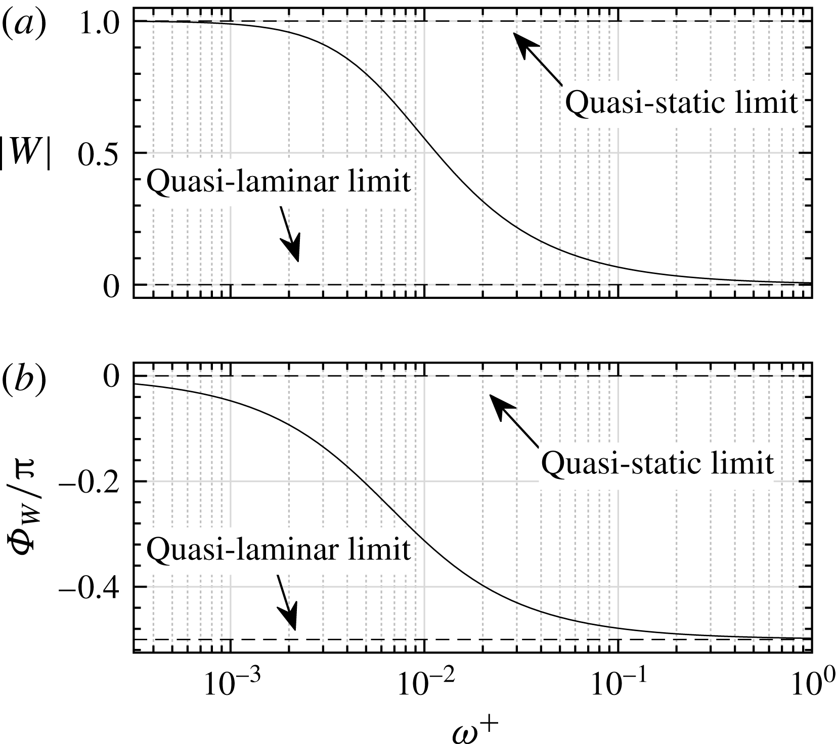
To examine whether this behaviour described by the NEM is physical, we study the amplitude of
 $\widetilde{r}$
obtained from the DNS. Figure 20 shows the comparison between the DNS data and the models. Apparently, the level of the perturbation Reynolds stress indeed decreases as the frequency increases, indicating that the turbulent diffusion of the perturbation field becomes insignificant as the flow approaches the highly non-equilibrium state. This phenomenon is not described by the QSM, as that model overestimates the turbulent stress at high frequencies, especially in the case of
 ${\it\omega}_{f}^{+}=0.04$
. Such overestimation of the turbulent stress is a typical problem with turbulence models that neglect the non-equilibrium effects in unsteady turbulent flows (Revell et al.
Reference Revell, Benhamadouche, Craft and Laurence2006). In comparison, the NEM gives a good prediction of the Reynolds stress level at higher frequencies, due to its inclusion of the non-equilibrium response of the Reynolds stress to the applied strain rate.
However, the NEM only gives qualitative agreement with the DNS. The first reason for this is the inaccuracy of the modelling due to the use of a spatially constant time scale
 $t_{T}$
, a fact that is discussed in detail later in this subsection. The second reason might be that the nonlinear effects are neglected in the linear NEM equation (4.5). As has been shown in § 3.4.2, nonlinear effects are at an observable level in the simulated pulsating flow. Therefore, the perturbation Reynolds stress
 $\widetilde{r}$
from the DNS may contain nonlinear contributions, which cannot be described by the linear model. The third reason might be the coexistence of other mode(s) apart from the shear wave. This (these) mode(s) may respond to the pulsating forces in a way that the linear perturbation equation (2.5) is unable to describe. The second and third reasons could also be the ones that cause the QSM to depart from the DNS results in the nearly quasi-static state (
 ${\it\omega}^{+}=0.001$
) in figure 20.
The amplitude of the perturbation Reynolds stress
 $\widetilde{r}$
as a function of
 $y^{+}$
: (a)
 ${\it\omega}_{f}^{+}=0.001$
, (b)
 ${\it\omega}_{f}^{+}=0.003$
, (c)
 ${\it\omega}_{f}^{+}=0.006$
, (d)
 ${\it\omega}_{f}^{+}=0.01$
, (e)
 ${\it\omega}_{f}^{+}=0.02$
, (f)
 ${\it\omega}_{f}^{+}=0.04$
.

The phase difference between the perturbation Reynolds stress
 $-\widetilde{r}$
and the shear strain rate
 $\partial \widetilde{u}/\partial y$
derived from the DNS data as a function of
 $y^{+}$
. It should be noted that the value of
 $\partial \widetilde{u}/\partial y$
approaches zero close to the channel centre, and then the phase of it is not defined and numerical errors occur. The errors are marked by the dotted lines.

Among the abovementioned three reasons, the first one is the easiest to quantitatively survey by using the DNS data. We will next examine whether the phase difference
 ${\it\Phi}_{W}$
, which is related to time scale
 $t_{T}$
by (4.7), is described correctly by the NEM. The values of
 ${\it\Phi}_{-\widetilde{r}}$
and
 ${\it\Phi}_{\partial \widetilde{u}/\partial y}$
in (4.8) can be individually obtained from the DNS data, and hence the value of
 ${\it\Phi}_{W}$
can be derived. Figure 21 shows the phase difference
 ${\it\Phi}_{W}$
derived from the DNS data for the six pulsating frequencies as a function of the wall distance
 $y^{+}$
. Since both
 $\widetilde{r}$
and
 $\partial \widetilde{u}/\partial y$
are close to zero near the channel centre, their phases are sensitive to turbulent noise and hence much less symmetric about the channel centreline than the data near the wall. These less accurate phases are marked by dotted lines in the figure.
Figure 21 reveals two main features of the phase differences that differ from the proposed NEM. First, the phase differences
 ${\it\Phi}_{W}$
seem not to be monotonically decreasing with the frequency. Although for the cases of
 ${\it\omega}_{f}^{+}=0.001$
to
 $0.02$
the phase differences somewhat confirm the decreasing trend near the wall, the case of
 ${\it\omega}^{+}=0.04$
seems to indicate the return of
 ${\it\Phi}_{W}$
back to zero. This result significantly differs from what is predicted by the NEM (see figure 19). One possible explanation is that the phase lag between the responding stress and the applied strain rate might be more than one cycle near the wall; therefore the
 ${\it\Phi}_{W}$
in figure 21 should be shifted
 $2{\rm\pi}$
downward instead. This explanation complies with the intuitive reasoning that the phase lag should increase with the pulsating frequency; it, however, becomes unconvincing if we look at the similarity in the spatial distributions of
 ${\it\Phi}_{W}$
between
 ${\it\omega}_{f}^{+}=0.04$
and the two lowest-frequency cases. The similarity indicates that the response of the stress to the applied pulsating strain rate may have similar time-lagging patterns at the low and the high frequencies, but the reason for this phenomenon is not fully understood and more investigations are needed.
The second feature revealed by figure 21 is the spatial dependence of the phase difference
 ${\it\Phi}_{W}$
, i.e. the phase difference varies in the wall-normal direction. Such a spatial dependence apparently opposes the assumption made in the NEM that the turbulent time scale
 $t_{T}$
, and hence the phase difference
 ${\it\Phi}_{W}$
, is spatially constant. The conflict between the assumption and the DNS data is not surprising, since the validity of the constant time scale is expected only in the near-wall region. According to the DNS the region where the constant-time assumption is potentially valid is limited to
 $y^{+}\lesssim 10$
, and this region shrinks as the frequency increases. Even so, the near-wall values are not accurately predicted by (4.4). Table 3 shows the values of
 ${\it\Phi}_{W}$
calculated from the time scale formula (4.4). Compared with the DNS results in figure 21, the predicted value of
 ${\it\Phi}_{W}$
seems to be valid in the near-wall region only for the cases of
 ${\it\omega}_{f}^{+}=0.001$
,
 $0.003$
and
 $0.006$
. For the other cases large discrepancies are observed between the model and the DNS, and in the cases of
 ${\it\omega}^{+}=0.01$
and 0.02 the DNS results close to the wall are even out of the range predicted by the model (0 to
 $-{\rm\pi}/2$
in radians).
It is interesting to note that the phase characteristics shown in figure 19 are consistent with observations in the study of homogeneous turbulence subject to periodic shear (Yu & Girimaji Reference Yu and Girimaji2006). Therefore, the two abovementioned major disagreements between (4.7) and the DNS may be attributed to the high wall-normal inhomogeneity of the channel flow. Detailed explanation of how the inhomogeneity would influence the phase lag between the stress and the strain requires further investigation. Despite such disagreements, the success of the NEM in the prediction of the wall shear stress in the intermediate frequency interval (see figure 16) somehow indicates that the time scale estimation equation (4.4) is quite compatible with the linear NEM in the near-wall region, being able to describe the pulsating boundary layer accurately enough. The need for adjusting the time scale is more urgent for the outer-layer performance, as indicated by figure 17. Such an adjustment is discussed in the next subsection.
Phase differences between the perturbation Reynolds stress
 $-\widetilde{r}$
and the shear strain rate
 $\partial \widetilde{u}/\partial y$
computed from the NEM, i.e. (4.7) with the estimated time scale (4.4), and from the wall values of the DNS data, i.e. the values in the neighbourhood of
 $y=0$
as shown in figure 21.

The amplitude of
 $\partial \widetilde{u}/\partial y$
at the channel wall, derived from the DNS data, and the NEM computed with the
 $y$
-dependent/independent
 $t_{T}$
. The
 $y$
-dependent
 $t_{T}$
is computed from the DNS of the phase difference
 ${\it\Phi}_{W}$
(see figure 21). The values in parentheses are the errors relative to the DNS data.

4.3 Attempt to improve the proposed turbulence model
In this subsection, the possibility of improving the NEM by using a more realistic turbulent relaxation time scale is discussed. To this end, the values of
 ${\it\Phi}_{W}$
from the DNS (see figure 21) are used to compute
 $t_{T}$
via (4.7), i.e.
 $t_{T}=-\!\tan ({\it\Phi}_{W})/{\it\omega}$
. Then, the computed time scale is used in the NEM equation (4.5) to calculate the perturbation velocity
 $\widetilde{u}$
, and the performance of the modified model in the inner and outer layers is re-examined.
First, the inner-layer performance is checked by evaluating
 $\partial \widetilde{u}/\partial y$
at the channel wall. Table 4 shows the amplitude of
 $\partial \widetilde{u}/\partial y$
computed from the DNS data and from the NEM with
 $y$
-dependent and spatially constant time scale respectively. Unfortunately, the comparison in table 4 shows that the
 $y$
-dependent time scale fails to provide systematic improvement of the model in the inner layer, with an evident improvement only for
 ${\it\omega}_{f}^{+}=0.01$
. In the cases of
 ${\it\omega}_{f}^{+}=0.001,0.003$
and 0.006 it deviates from the DNS even more than the values computed with the spatially constant time scale. This observation shows that the time scale equation (4.4) is in general compatible with the linear relaxation model equation (4.3) in the inner layer. However, improvement is found in the phase profile for the cases of
 ${\it\omega}_{f}^{+}=0.001,0.003$
and 0.006, see figure 22, where the ‘V’ shape in the phase near the wall, which is only observable in these three frequency cases, is significantly better predicted by applying the
 $y$
-dependent
 $t_{T}$
.
(a) The amplitude of the perturbation velocity
 $\widetilde{u}$
and (b) the phase lead (rad) of the perturbation velocity
 $\widetilde{u}$
to its centreline value
 $\widetilde{u}_{\mathit{cl}}$
for the six forcing frequencies
 ${\it\omega}_{f}^{+}=0.001$
to 0.04: ——, NEM with constant
 $t_{T}$
; — ⋅ —, NEM with
 $y$
-dependent
 $t_{T}$
;
 $\circ$
, DNS.

Second, the outer-layer performance is evaluated by inspecting whether the problem of the incorrectly predicted shear wave propagation (see § 4.2.1) is suppressed. The profiles of the perturbation velocity
 $\widetilde{u}$
are presented in figure 22. Clear improvements are found for all six frequencies, where the damping coefficient and the wavelength of the shear wave are better predicted by using the
 $y$
-dependent
 $t_{T}$
compared with the spatially constant one. We then conclude that the results shown in figure 22 open the possibility of improving the NEM by using a spatial-dependent relaxation time
 $t_{T}$
, but the derivation of a formula for such
 $t_{T}$
is non-trivial. As has been shown in figure 21, there seems to be no similarity in the spatial distribution of
 $t_{T}$
at different frequencies in general; therefore, data for
 $t_{T}$
at more frequencies have to be acquired to search for the distribution pattern of
 $t_{T}$
. Even so, the acquired data cannot be applied to fit
 $t_{T}$
without further tuning, as table 4 shows that applying the data from the DNS directly to
 $t_{T}$
, and hence to the NEM, will not fill the gap between the predicted results and the DNS.
4.4 Dependence on the Reynolds number
As has been pointed out in § 4.2.1, the Reynolds number is found to be an issue that may influence the behaviour of the pulsatile flow. The main reason is that at low Reynolds numbers the gap between the shear wave boundary layer edge and the turbulent outer-layer portion becomes narrow, and then at low frequencies the shear wave may intrude beyond the channel centre and possibly interfere with the shear wave originating from the opposite channel wall. Such an intrusion is well visualized in figure 22, where the noticeable deviation of the centreline velocity magnitude from its expected value,
 $a_{\mathit{cl}}=0.1$
, clearly indicates that the shear wave reaches the channel centre before it dies out. The thickness of the shear wave boundary layer can be estimated by the Stokes length
 $l_{\mathit{s}}^{+}$
. Then, the onset of the intrusion is determined by the ratio
 $l_{\mathit{s}}^{+}/Re_{{\it\tau}}$
, i.e. the outer layer of the shear wave would be Reynolds-number-independent when
 $l_{\mathit{s}}^{+}/Re_{{\it\tau}}\ll 1$
.
A more interesting question is whether such Reynolds number dependence can influence the near-wall behaviour of the pulsatile flow, i.e. whether the wall shear stress impedance
 $\widetilde{{\it\tau}}_{\mathit{w}}$
in figure 16 also becomes Reynolds-number-dependent at low Reynolds numbers. Ronneberger & Ahrens (Reference Ronneberger and Ahrens1977) suggest a ‘critical’ length scale
 $l_{\mathit{s,c}}^{+}$
, such that
 $\widetilde{{\it\tau}}_{\mathit{w}}$
at most weakly depends on the Reynolds number when the ratio
 $l_{\mathit{s}}^{+}/l_{\mathit{s,c}}^{+}$
is much smaller than one, and this ratio is given by
 $$\begin{eqnarray}\frac{l_{\mathit{s}}^{+}}{l_{\mathit{s,c}}^{+}}\approx \frac{2}{3}\sqrt{\frac{1}{2}\frac{1}{{\it\omega}^{+}Re_{{\it\tau}}}\sqrt{\frac{8}{c_{f}}}},\end{eqnarray}$$
where
 $c_{f}$
is the friction factor. If we use the Prandtl friction law for
 $c_{f}$
in fully developed pipe flows (Pope Reference Pope2000),
 $$\begin{eqnarray}\sqrt{\frac{8}{c_{f}}}=\frac{1}{{\it\kappa}}\ln Re_{{\it\tau}}+B,\end{eqnarray}$$
with
 $$\begin{eqnarray}B=\frac{1}{{\it\kappa}}\ln 4\sqrt{2}-\frac{3+5\ln 2-2{\it\kappa}B_{\mathit{P}}}{2{\it\kappa}},\end{eqnarray}$$
where
 ${\it\kappa}=0.41$
and
 $B_{\mathit{P}}=5.2$
, we can deduce that the near-wall behaviour of the shear wave can be treated as uninfluenced by the outer layer if the pulsating frequency satisfies the following relation:
 $$\begin{eqnarray}{\it\omega}^{+}\gg \frac{2}{9}\frac{1}{Re_{{\it\tau}}}\left(\frac{1}{{\it\kappa}}\ln Re_{{\it\tau}}+B\right)\approx 0.01,\end{eqnarray}$$
where
 $Re_{{\it\tau}}=350$
is used.
The frequencies
 ${\it\omega}_{f}^{+}=0.001$
–0.006 used in our DNS are smaller than the critical frequency in (4.12); therefore the obtained wall shear stresses
 $\widetilde{{\it\tau}}_{\mathit{w}}$
at these forcing frequencies, as shown in figure 16, are probably different from the data obtained for higher Reynolds numbers.
5 Conclusion and outlook
Direct numerical simulation of a turbulent channel flow (
 $Re_{{\it\tau}}=350$
) subjected to superimposed sinusoidal oscillations with different frequencies has been performed. The parameters used in the DNS have covered a significant range of dimensionless frequencies
 ${\it\omega}^{+}$
, including the intermediate frequency range (see table 2). The perturbation amplitude has been controlled such that the mean flow statistics remain uninfluenced by the imposed oscillation.
The DNS results have been compared with an NEM. In this model the dynamics of the perturbation Reynolds stress is expressed by a linear relaxation equation. It is based on the assumption that the turbulent mixing of the perturbation field in the quasi-static state can be described by an eddy viscosity. Unlike quasi-static approaches, this model considers the non-equilibrium effects during the response of the perturbation Reynolds stress to the applied perturbation shear. Therefore, the model is able to predict the phase lag between the stress and the shear strain rate when the pulsation frequency increases. According to the model, the turbulent eddies behave in a viscoelastic manner in the intermediate frequency range. This is believed to be the reason for the reduced perturbation wall shear stress compared with its laminar value (see figure 16 a).
Some main observations and conclusions are summarized as follows.
First, the DNS shows that the perturbation field contains fundamental frequency components (resulting from the imposed forcing) as well as higher harmonic components. The latter components are caused by nonlinear effects during the production and transportation of the perturbation Reynolds stresses. In the present study the maximum nonlinear effects are found for the case of
 ${\it\omega}_{f}^{+}=0.006$
. The reason behind this behaviour is not yet clear. In addition, the amplitudes of the fundamental modes in the perturbation Reynolds stresses,
 $\widetilde{r}$
,
 $\widetilde{v^{\prime }v^{\prime }}$
and
 $\widetilde{w^{\prime }w^{\prime }}$
, monotonically decrease as the frequency increases, except for the normal stress component,
 $\widetilde{u^{\prime }u^{\prime }}$
, which shows increase in the cases of
 ${\it\omega}_{f}^{+}=0.006$
and 0.01.
Second, the DNS shows that in the cases of
 ${\it\omega}_{f}^{+}=0.01$
, 0.02 and 0.04, the shear wave decays more slowly than in quasi-laminar flow (see figure 18), i.e. the damping coefficient of the shear wave is reduced by the turbulent flow. This observation supports the NEM that the turbulent eddies behave viscoelastically, and it is this elastic behaviour that tends to reduce the damping coefficient of the shear wave. The predicted viscoelasticity agrees with the fact that the perturbation wall shear stress is smaller than its quasi-laminar value in the intermediate frequency range (see figure 16). The elasticity of the eddies also causes the shear wave boundary layer to be thicker than in a purely viscous flow.
Third, the amplitude of the perturbation Reynolds stress
 $\widetilde{r}$
obtained from the DNS is shown to decrease as the pulsation frequency increases. This confirms the prediction by the NEM that the level of the perturbation Reynolds stress is reduced when the non-equilibrium state is reached. Moreover, the observed phase lag between the perturbation Reynolds stress and the shear strain rate further proves that the response of the background turbulence to the imposed oscillation is not in equilibrium. The degree of the non-equilibrium is inhomogeneous across the boundary layer, indicating that the turbulent relaxation time for a given pulsation frequency depends on the distance from the wall.
In general, the performance of the proposed non-equilibrium model is good in the near-wall region for the whole frequency span, as the wall shear stress of the perturbation field is well predicted by the model. However, the model only shows qualitative agreement with the DNS data in the outer layer. We have replaced the spatially constant relaxation time in the original model by the spatial-dependent relaxation time obtained from the DNS, in the hope of improving the model. This attempt produced an overall improvement in the outer layer, but failed to improve the model in the near-wall region. Future attempts could focus on including nonlinear effects in the modelling, to yield a more complete description of the perturbation field.
Besides the linear models discussed in this paper, other more complete Reynolds stress transport models, such as the LRR model developed by Launder, Reece & Rodi (Reference Launder, Reece and Rodi1975) or the SSG model developed by Speziale, Sarkar & Gatski (Reference Speziale, Sarkar and Gatski1991), naturally capture non-equilibrium, nonlinear and transport effects, and have been shown to be fairly accurate in non-pulsating channel flows. Examination of the performance of these transport models in pulsating flows by URANS-based simulations could be part of future studies.
In addition, at very high frequencies (
 ${\it\omega}^{+}>0.04$
), some authors have speculated on a possible resonance with the ejection/bursting mechanism in the near-wall layer. It would be interesting to explore this frequency regime as well.
Acknowledgements
The authors are grateful to Dr P. Schlatter for fruitful discussions and guidelines regarding the SIMSON code. Computer time provided by SNIC (Swedish National Infrastructure for Computing) is gratefully acknowledged. This work was funded by VR (the Swedish Research Council) and by the Linné FLOW Centre at KTH.
Appendix A
In this paper, we use the algebraic model proposed by She et al. (Reference She, Wu, Chen and Hussain2012) to compute the eddy viscosity
 ${\it\nu}_{T}$
. The details of the model are given below. The eddy viscosity is written as
 $$\begin{eqnarray}{\it\nu}_{T}(Re_{{\it\tau}},y^{+})=l_{\mathit{m}}^{+2}|S^{+}|,\end{eqnarray}$$
where the dimensionless mixing length
 $l_{\mathit{m}}^{+}$
for the channel flow is given by
 $$\begin{eqnarray}\displaystyle l_{\mathit{m}}^{+}(Re_{{\it\tau}},y^{+}) & = & \displaystyle {\it\varrho}\left(\frac{y^{+}}{y_{\mathit{sub}}^{+}}\right)^{3/2}\left[1+\left(\frac{y^{+}}{y_{\mathit{sub}}^{+}}\right)^{4}\right]^{1/8}\left[1+\left(\frac{y^{+}}{y_{\mathit{buf}}^{+}}\right)^{4}\right]^{-1/4}\nonumber\\ \displaystyle & & \displaystyle \times \,\frac{1-(1-y)^{4}}{4yZ_{\mathit{core}}}\left[1+\left(\frac{1-y}{y_{\mathit{core}}}\right)^{-2}\right]^{1/4}.\end{eqnarray}$$
The coefficients in (A 2) are given by
 $$\begin{eqnarray}\displaystyle \left.\begin{array}{@{}c@{}}{\it\varrho}={\it\varrho}_{0}(1+{\it\varepsilon}_{{\it\varrho}}),\quad {\it\varrho}_{0}={\displaystyle \frac{2^{3/8}\sqrt{5}}{3}},\quad y_{\mathit{sub}}^{+}=\left({\displaystyle \frac{0.0315}{{\it\varrho}_{0}}}\right)^{-2/3},\\ y_{\mathit{buf}}^{+}=44.7(1-{\it\varepsilon}_{{\it\varrho}}),\quad Z_{\mathit{core}}=(1+y_{\mathit{core}}^{2})^{1/4},\quad y_{\mathit{core}}=0.67(1-{\it\varepsilon}_{c}),\\ {\it\varepsilon}_{{\it\varrho}}=\left\{\begin{array}{@{}ll@{}}0.1{\displaystyle \frac{5000-Re_{{\it\tau}}}{4000}},\quad & Re_{{\it\tau}}\leqslant 5000,\\ 0,\quad & Re_{{\it\tau}}>5000,\end{array}\right.\quad {\it\varepsilon}_{c}=\left\{\begin{array}{@{}ll@{}}0.6{\displaystyle \frac{5000-Re_{{\it\tau}}}{4000}},\quad & Re_{{\it\tau}}\leqslant 5000,\\ 0,\quad & Re_{{\it\tau}}>5000.\end{array}\right.\end{array}\right\} & & \displaystyle \nonumber\\ \displaystyle & & \displaystyle\end{eqnarray}$$
The dimensionless mean shear strain rate
 $S^{+}$
is expressed in terms of
 $l_{\mathit{m}}^{+}$
as
 $$\begin{eqnarray}S^{+}=\frac{-1+\sqrt{4(1-y)l_{\mathit{m }}^{+2}+1}}{2l_{\mathit{m}}^{+2}}.\end{eqnarray}$$
Using (A 1), the mean flow velocity
 $\overline{u}$
can be obtained by solving (2.3) numerically.