INTRODUCTION
Galician coastal waters (north-west Spain) are characterized by high biodiversity and productive fisheries, supported by nutrient input due to upwelling (e.g. Varela et al., Reference Varela, Diaz del Rio, Alvarez-Ossorio and Costas1991). Twenty species of cetaceans have been recorded in Galician waters, of which the most abundant appear to be short-beaked common dolphins (Delphinus delphis) and, in the coastal rías, bottlenose dolphins (Tursiops truncatus). Other species present in the area include harbour porpoises (Phocoena phocoena), Risso's dolphins (Grampus griseus) and long-finned pilot whale (Globicephala melas) (Cendrero, Reference Cendrero1993; López et al., Reference López, Santos, Pierce, González, Valeiras and Guerra2002, Reference López, Pierce, Valeiras, Santos and Guerra2004).
Under Annex II of the European Union Habitats and Species Directive (92/43/EEC), bottlenose dolphins and harbour porpoises are considered priority species for conservation in European waters. Both Spanish and Galician law also recognize the need to protect cetaceans and establish the legal basis for their conservation in Galician waters. The law on conservation of wild areas and species (4/1989) established a national catalogue of threatened species, with some cetacean species being included from June 1999. The list of species was further revised in 2000 and 2006. The law on conservation of nature (9/2001) set out rules for protection, conservation and restoration of natural resources and the management of wild habitats and species. In 2001 the Galician government established a catalogue of threatened species in Galicia. The law on natural heritage and biodiversity (42/2007) included the transposition of the Habitats Directive into Spanish law. The Galician decree 88/2007 aimed to prevent the loss of biodiversity, focusing on species listed as threatened. The Royal decree 1727/2007 has the objective of putting in place measures for the protection of cetaceans in Spanish waters to ensure their survival and favourable conservation status.
Conservation issues for cetaceans in Galician waters include interactions with fisheries, which may be a significant cause of mortality (López et al., Reference López, Santos, Pierce, González, Valeiras and Guerra2002, Reference López, Pierce, Santos, Gracia and Guerra2003a), overfishing, and oil spills. Vieites et al. (Reference Vieites, Nieto-Roman, Palanca, Ferrer and Vences2004) identified the European Atlantic, especially the English Channel and Galician coast (most recently affected by the ‘Prestige’ oil spill in 2002), as a major hotspot for oil spills—although it should be noted that Ridoux et al. (Reference Ridoux, Lafontaine, Bustamante, Caurant, Dabin, Delcroix, Hassani, Meynier, da Silva, Simonin, Robert, Spitz and Van Canneyt2004) found no evidence of effects on marine mammals from the ‘Erika’ oil spill on the French coast.
Monitoring of cetacean strandings in Galicia has been undertaken since 1990 by the non-governmental organization Coordinadora para o Estudio dos Mamíferos Mariños (CEMMA; see López et al., Reference López, Santos, Pierce, González, Valeiras and Guerra2002). Two recent large-scale European-funded cetacean sightings surveys (SCANS II in 2005 and CODA in 2007) extended into inshore and offshore waters of Galicia respectively, although neither surveyed the interior waters of the coastal rías. CEMMA also carries out both dedicated and opportunistic cetacean sightings surveys in continental shelf waters of Galicia, for example by placing observers on-board fishing or coastguard vessels (see López et al., Reference López, Cedeira, Caldas, Carril, Solla and Llavona2003b, Reference López, Pierce, Valeiras, Santos and Guerra2004). A range of other studies, for example on diet and contaminant burdens (González et al., Reference González, López, Guerra and Barreiro1994; Santos et al., Reference Santos, Pierce, López, Martínez, Fernández, Ieno, Mente, Porteiro, Carrera and Meixide2004, Reference Santos, Fernández, López, Martínez and Pierce2007; Lahaye et al., Reference Lahaye, Bustamante, Law, Learmonth, Santos, Boon, Rogan, Dabin, Addink, López, Zuur, Pierce and Caurant2007; Pierce et al., Reference Pierce, Santos, Murphy, Learmonth, Zuur, Rogan, Bustamante, Caurant, Lahaye, Ridoux, Zegers, Mets, Addink, Smeenk, Jauniaux, Law, Dabin, López, Alonso Farré, González, Guerra, García-Hartmann, Reid, Moffat, Lockyer and Boon2008) and population structure (e.g. Murphy et al., Reference Murphy, Herman, Pierce, Rogan and Kitchener2006) have built on data and samples collected by CEMMA.
Prior to 2003 there were no systematic coastal surveys of cetaceans in Galicia. The present study was instigated by CEMMA in September 2003 to provide baseline data on the cetacean species present in coastal waters, their distribution, abundance and habitat use. This is particularly important in the interior waters of the Galician rías and in shallow coastal waters over rocky bottoms which are not accessible to larger survey boats. The information collected will inform conservation plans by identifying coastal areas of high importance to cetaceans.
In recent years, numerous authors have used survey data from a range of sources to model habitat use by cetaceans (see Redfern et al., Reference Redfern, Ferguson, Becker, Hyrenbach, Good, Barlow, Kaschner, Baumgartner, Forney, Ballance, Fauchald, Halpin, Hamazaki, Pershing, Qian, Read, Reilly, Torres and Werner2006 for a review). Land-based sightings are clearly restricted in that only areas visible from the coast can be surveyed but they offer the opportunity to cover coastal waters relatively inexpensively, and to provide standardized, effort-based data on species presence and relative abundance in coastal waters (Evans & Hammond, Reference Evans and Hammond2004). While prey distribution and abundance are widely cited as among the most important factors affecting cetacean distribution, it is also apparent that it can be more efficient to use oceanic and other physical environmental characteristics as proxies for local prey abundance (Torres et al., Reference Torres, Read and Halpin2008) and indeed there may be direct effects of environmental conditions on cetacean distribution. Such research is facilitated by the ready availability of spatially referenced bathymetry data and satellite imagery, from which parameters such as sea surface temperature (SST) and surface chlorophyll-a concentration (chl-a, a measure of primary productivity) can be estimated (see Valavanis et al., Reference Valavanis, Pierce, Zuur, Palialexis, Saveliev, Katara and Wang2008 for a recent review).
In the present paper, we analyse spatial and temporal (seasonal and interannual) patterns in sightings rates for the main cetacean species present along the Galician coast and examine the possible relationships of these patterns with environmental conditions.
Although the surveys were systematic in the sense that sampling was carried out monthly over a period of four years, the number of sites visited was reduced from 53 to 30 in the final calendar year of the study (while retaining coverage of the whole coastline) due to resource constraints, and time spent observing at sites has varied (although 98% of observation periods were between 20 and 60 minutes duration). Therefore, we also carried out analyses to determine an effective sampling strategy. Although the best strategy undoubtedly depends on the precise research goals, we argue that maximization of average sightings rate for the main species while retaining a good spatial and temporal coverage of the area is a reasonable goal, and therefore investigate the optimal numbers of site visits and optimal time spent at each site under this premise.
MATERIALS AND METHODS
Data collection
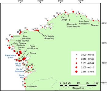
Systematic monthly sightings surveys for cetaceans were carried out in Galicia (north-west Spain) under the auspices of CEMMA, from a series of 30 core sites spread approximately evenly along the entire Galician coastline. The aim was to visit each site at least once during every month. Surveys commenced in September 2003 and the present analysis includes data collected up to October 2007 (i.e. around 50 visits per site): in practice the total number of visits to these sites over the study period ranged from 36 to 121 (median 49). An additional 23 observation sites were visited approximately monthly until the end of 2006: for these sites, the total number of visits ranged from 25 to 62 (median 37). All 53 locations are shown in Figure 1.
Observation points (numbered NE to SW, 1 to 53) and average probability of cetacean sightings (proportion of observation periods during which cetaceans were seen, all species combined), September 2003–October 2007.

Observers (usually 2, range 1 to 9 people) scanned continuously using telescopes and binoculars. At least one experienced observer was present during all observation periods. The modal observation duration was 30 minutes, with around 1/3 of all observation periods lasting 30 minutes, and 98% of observation periods lasted between 20 and 60 minutes (range 7–215 minutes). Observers recorded the time at which observations started and finished, and all cetacean sightings. For each group of cetaceans seen, observers recorded the species, group size, time and duration of sighting, and descriptions of behaviour, including whether the spacing of individuals was compact or dispersed (or mixed) and whether the animals showed directional movement or remained in the same area (or a mixture of both).
Observers also recorded a series of environmental parameters, including visibility (on a scale of 0 to 5 where 0 is dense fog and 5 is visibility of more than 10 miles), sea state (Douglas scale), wind strength (Beaufort scale) and direction, and estimates of the depth of the field of view and the angle describing the field of view (from which the observation area was calculated). For each site, latitude, longitude and height of the observation position are known. Most observations took place between 10.00 and 20.00 h.
BATHYMETRY AND REMOTELY-SENSED ENVIRONMENTAL DATA
Bathymetry data were derived from the General Bathymetric Chart of the Oceans (GEBCO, http://www.gebco.net). The width of the continental shelf at each observation point (coast to 200 m isobath) was estimated using GIS software and may be considered as a proxy for average seabed depth and slope in the vicinity of the observation point.
Sea surface temperature and chl-a data for every project month during 2003–2006 were derived from satellite images. Coastal waters were divided into ten zones and, in each zone, data were extracted for a transect running from the 100 m to the 1000 m isobaths. Satellite imagery cannot be used to derive reliable SST and chl-a values immediately adjacent to the coast and no data for 2007 were available at the time the analysis was carried out. SST and chl-a data from each transect were assumed to be applicable to adjacent areas. Thus the resolution of temporal and spatial variation in oceanographic conditions is relatively coarse but use of 10 transects per month represented a compromise between resolution and coverage. For smaller areas and shorter time periods, missing data (mainly due to cloud cover) were an issue. Both minimum and maximum SST and chl-a values were available for analysis. Since SST and chl-a show clear seasonal cycles, these values were converted to spatial and annual anomalies by firstly calculating monthly means (i.e. averaging values across all 10 transects in all 3 years separately for each month) and then subtracting the relevant monthly mean from all individual values in that month.
Data processing
Sightings data (N = 2464 observation periods) were initially summarized by project year and calendar month. Project year 1 ran from September 2003–August 2004 and the study extended two months into the fifth year.
Wind direction, being a circular variable, was re-coded into easterly and northerly components, i.e. the sine and cosine of the angle (in radians). The number of observers was usually between 1 and 3 (maximum 9) and was therefore coded as 1, 2, 3 and 3+. The area covered by the field of view (FOV) was estimated using simple trigonometry as:

Project year, number of observers, wind direction, visibility and sea state were treated as categorical explanatory variables. Month and wind strength were treated, for convenience, as continuous explanatory variables. Observation start time, observation duration, FOV area, SST, chl-a and shelf width were all treated as continuous explanatory variables.
Analysis of spatial and temporal trends in sightings
For this analysis, data for project year 5 (i.e. the last two months of data collected) were excluded to ensure a balanced coverage of the calendar year. The statistical distribution of numbers of animals sighted per observation period was highly skewed with many zero values. A two-stage analysis of temporal and spatial trends was therefore carried out, with the response variables being presence and numbers of animals sighted (given presence), respectively. Since the shapes of relationships with explanatory variables were unknown, generalized additive models (GAMs) were used. Explanatory variables included measures of observation effort (observation period, FOV area and number of observers), weather (wind speed and direction, sea state and visibility) and the time of day at which observations started. The spatial pattern was modelled by treating position along the coast as a continuous uni-dimensional explanatory variable, numbering the observation points from 1 to 53 from the north to the south. Binomial GAMs were used for modelling presence. For numbers of animals seen (given presence), quasi-Poisson models were used, i.e. assuming a Poisson distribution with an additional parameter to allow for overdispersion.
Models were constructed by a combination of forwards and backwards selection, removing terms that were clearly non-significant (P ≫ 0.05). To assist with the selection process we used the ‘basis = cs’ option for fitting smoothers, which allows degrees of freedom for individual smoothers to fall to zero (a good indication of non-significance). If the final value for degrees of freedom of a smoother was around 1.0, i.e. the fit was approximately linear, we replaced the smoother with a linear term. Having reached a ‘final’ model, we checked whether it could be improved by adding any of the explanatory variables absent from the model. The final model was the model with the lowest Akaike information criterion given that effects of all explanatory variables retained in the model were statistically significant and there were no clear patterns in the residuals. Once wind speed was included in the models, the effect of sea state was never significant and no effect of wind direction was detected. For all continuous explanatory variables except position along the coast, smoothers were constrained to a maximum k value of 4 (i.e. a maximum of 3 degrees of freedom), thus limiting relationships to plausible simple forms and avoiding overfitting. All models were fitted using BRODGAR 2.6.5 software (www.brodgar.com), a menu-based R interface (using R 2.9.1).
Analysis of habitat preferences
The model fitting process described above was repeated, excluding year and location as explanatory variables but adding the environmental variables SST anomaly, chl-a anomaly and shelf width. For this analysis, only data for 2004–2006 were used, ensuring balanced coverage of the calendar year. If the variable ‘month’ did not figure in the final model, SST and chl-a anomaly series were replaced by the original data series. For both SST and chl-a, minima and maxima were highly collinear and in every analysis we therefore selected whichever of the two was more closely related to the response variable.
An implicit assumption of this second stage of the modelling process is that spatial and interannual variation in sightings rate was a consequence of environmental variation. If resulting models are clearly less satisfactory than models in which spatial and interannual variation is explicitly modelled, it may be concluded that such variation is not entirely due to variation in the environmental parameters studied. Similar to the models of spatiotemporal variation, smoothers for all continuous explanatory variables except month and time of day were constrained to a maximum k value of 4.
Survey efficiency
We quantified the relationships between mean sightings rates and observation duration, with the expectation that short sampling periods would tend to result in lower sightings rate estimates and that sightings rate would tend to reach an asymptote for longer observation periods (i.e. once observation duration exceeds the average interval between sightings). Cleary mean sightings rate or number of sightings per unit effort (SPUE, animals per hour) depends on which subset of the data is used. Here we derived a series of new SPUE variables for each species by using observations of duration D to derive information on sightings rates for all durations up to D. Thus, for hypothetical observation period durations of d = 5, 10, 15, … , 60 minutes, SPUE was calculated as the number of animals seen per hour over the period 0 to d minutes, unless observers had stayed less than d minutes in which case SPUE was undefined (missing data). Thus if no animals were sighted until minute 14 of a 30-minute observation period, SPUE values for d = 5 minutes and d = 10 minutes would be zero, SPUE would be greater than zero for all subsequent d values up to 30 minutes, and SPUE would be undefined for d values greater than 30 minutes. Clearly, sample size declines for higher values of d, which must be taken into account in any comparison of SPUE across different d values. Furthermore, there may have been a tendency for observers to remain longer if animals were seen. Therefore, in determining the relationship between sightings rate and observation time for observation periods with durations of up to d = D minutes, to ensure an unbiased comparison we excluded all data for observation periods of duration less than D minutes. This exercise was repeated for D = 30 and 60 minutes.
We considered several possible criteria to identify the ‘optimum’ time to remain at an observation point. We compared histograms of observation durations and times of first sighting (‘waiting times’) for each species, based on subsets of site visits during which only one species was sighted. We examined the shape of the relationships between mean sightings rates and observation duration, looking for possible inflection points. We used bootstrapping to estimate confidence limits for sightings rates and looked for discontinuities in the relationships between confidence interval width and time-at-site. Lastly, by analogy with optimal patch use (Charnov, Reference Charnov1976), we estimated optimum waiting times to maximize sightings rate using a simple graphical method, based on information about average observer travel time between observation sites. Here, the asymptotic curve representing average sightings rate versus time spent at an observation site is analogous to the asymptotic curve representing cumulative energy intake from feeding in a patch as a function of residence time. A tangent is drawn from the point –t on the x axis, where t is the travel time, to intersect with the curve such that the overall sightings rate (number of animals sighted divided by the sum of travel and residence time) is maximized. Under the original sampling regime (53 mainland observation points), travel time is estimated to range from 25 to 100 minutes between sequential points (mean 56 minutes). After reduction to 30 core points, estimated travel times ranged from 30 to 120 minutes (mean 70 minutes). Hence we provide results for travel times between 30 and 120 minutes.
Finally, we used random sub-sets of data from observation periods of at least 30 minutes duration to examine how sightings rate varied in relation to the number of site visits carried out over the study period (i.e. the effect of sample size). Median and 95% confidence limits for each sample size (number of visits) were based on a bootstrap resampling procedure with 1000 repeats per sample size/observation time/species combination. The bootstrap routines were written using QuickBASIC.
RESULTS
Species present, general trends in sightings, behaviour
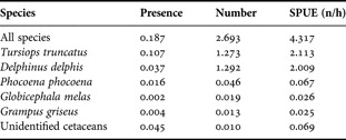
Cetaceans were seen all around the Galician coast but, overall, the highest frequency of sightings was at around 42.5° to 43°N (Figure 1). The proportion of observations during which sightings were made, the average number of animals seen per observation period and average sightings rate (animals.hour−1) are summarized in Table 1. The most frequently sighted species, bottlenose dolphin (Tursiops truncatus) was seen during 10.7% of observation periods as compared to 3.7% for common dolphin (Delphinus delphis), although numbers seen were slightly bigger for the latter species due to larger average group sizes. Porpoises (Phocoena phocoena) were seen during 1.6% of observations. Risso's dolphins (Grampus griseus) and short-finned pilot whales (Globicephala melas) were also occasionally seen while unidentified cetaceans were seen during 4.5% of observation periods (Table 1).
Overall sightings rates for all cetaceans by species: (a) presence (proportion of observation periods during which they were seen), (b) number (average number of animals seen per observation period) and (c) sightings rate (SPUE, average number of animals seen per hour), based on 2465 observation periods, September 2003–October 2007.

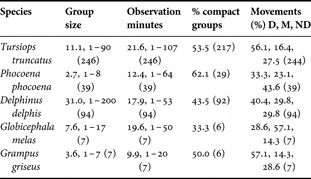
Average group size was highest in common dolphins. Both compact and dispersed groups were seen in all species, compact groups being relatively most common in harbour porpoises. Among the three most frequently seen species (there are few data for Risso's dolphins and pilot whales), the proportion of groups seen undertaking directional movement was highest in bottlenose dolphins, although groups of this species also tended to remain in view longest (Table 2). In general, bottlenose dolphins and harbour porpoises were seen to travel relatively slowly, with periods of travel interspersed with bouts of foraging, while common dolphins travelled relatively quickly (although this was not formally quantified).
Goup size and behaviour for the three main species: group size and duration of sightings of groups (mean, minimum and maximum), percentage of groups which comprised closely spaced animals and the percentage of groups seen undertaking directional movement (D), a mixture of directional and non-directional movements (M) and, only non-directional movements (ND). In all cases, the sample size (N) is given in parentheses.

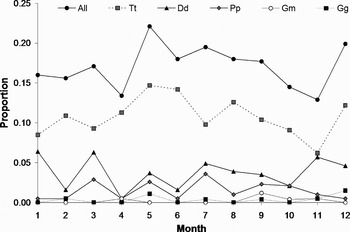
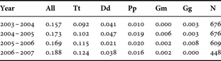
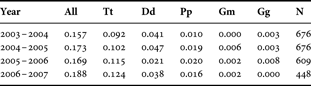
Uncorrected data on frequency of sightings suggest a seasonal peak in May. However, sightings were also high in July and December and there were differences between species (Figure 2). The data also suggest an increase in occurrence of bottlenose dolphins over time (Table 3). No clear trends are evident for the other species although no Risso's dolphins have been sighted since August 2006 (the last of 9 sightings during the study period).
Presence (proportion of observation periods during which cetaceans were seen) , by calendar month: all cetacean species (All), Tursiops truncatus (Tt), Delphinus delphis (Dd), Phocoena phocoena (Pp), Globicephala melas (Gm) and Grampus griseus (Gg). The highest rates are highlighted in bold. Monthly sample sizes (numbers of observation periods, N) were: 188, 192, 205, 186, 190, 183, 221, 206, 260, 241, 194 and 196.

Presence (proportion of observation periods during which cetaceans were seen) for all cetaceans and the main individual species, by project year: Tursiops truncatus (Tt), Delphinus delphis (Dd), Phocoena phocoena (Pp), Globicephala melas (Gm) and Grampus griseus (Gg). The table also indicates the sample size (N). Project years run from September to August.
Spatial and temporal variation in cetacean presence
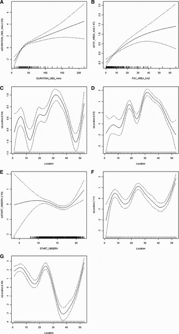
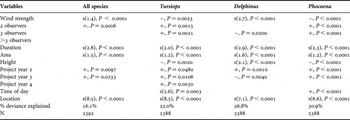
The final GAM for presence of cetaceans (pooled data for all species) indicated a linear increase in probability of sightings with increasing observation duration and area and a negative effect of increasing wind strength (up to around Beaufort 3). As observation area and duration increase, the increment in presence tends to level off (see Figure 3A, B). Once wind strength was included in the model, effects of visibility and sea state were not significant. The incidence of sightings was also greater when two observers were present, rather than one, but there was no significant gain from larger numbers of observers. Once these effects were taken into account, there was a tendency for increased sightings in the second and third project years compared to the first and a strong spatial pattern (Figure 3C) with a peak in sightings centred on observation point 32 (Castro de Baroña, Porto do Son), 42.70°N 9.03°W) and an additional peak around point 53, La Guardia in the far south of Galicia. There was no significant diurnal or month-to-month variation in the incidence of sightings. The model explained 16.1% of deviance in cetacean presence and is thus relatively weak (Table 4).
Generalized additive model results: smoothing functions for effects of duration of observation, field of view area, time of day and location on presence of cetaceans. The Y-axis represents the trend (positive or negative) in sightings rate. In the case of location, the X-axis indicates the observation points, numbered in sequence from 1 in the far north-east to 53 in the far south-west. Dotted lines are the approximate 95% confidence limits. (A) Effect of observation duration, all species combined; (B) effect of field-of-view area, all species; (C) effect of location, all species; (D) effect of location, Tursiops truncatus; (E) effect of time of day, Tursiops truncatus; (F) effect of location, Delphinus delphis; (G) effect of location, Phocoena phocoena.

Summary of generalized additive models for spatial and temporal patterns in presence of all cetacean species, Tursiops, Delphinus and Phocoena. For categorical explanatory variables, the effect given for each level is relative to a reference level (e.g. for number of observers, all comparisons are in relation to observation periods with one observer present). For each model, all significant explanatory variables are listed with their associated probability (P) value, along with the overall % deviance explained by the model and sample size (number of observation periods, N). For categorical and linear explanatory variables, the direction of the effect is indicated as + or –; for smoothers (s), the degrees of freedom are indicated in parentheses. Data for project year 5 (i.e. the last two months of the study) were excluded from this analysis to ensure a balanced coverage of the calendar year.

Final models for presence of the most frequently seen individual species are also summarized in Table 4. In all these models there were strong positive effects of longer observation duration and larger field-of-view areas and a generally negative effect of higher wind strength, although these effects were generally non-linear. In all cases, % deviance explained was over 20% and models can be considered satisfactory.
Tursiops truncatus was seen most frequently around observation point 32 and, to a lesser extent, point 18 (Punta Alta, Barrañán, Arteixo, 43.31°N 8.56°W; see Figure 3D) and there were significantly more sightings in the second, third and fourth project years than in the first year. There was a significant trend for more sightings to take place in the morning and evening and fewest around 16.00–17.00 h (Figure 3E) and a tendency for more sightings to be made from lower observation points. Sightings were more frequent when two or three observers were present, rather than one.
There were peaks in presence of Delphinus delphis centred around three observation points: 8 (Mirador de Santo Antonio, Ortigueira, 43.73°N 7.81°W), 25 (Cabo Touriñán, Muxia, 43.06°N 9.30°W) and 53 (La Guardia) (Figure 3F). There were more frequent sightings from higher observation points, up to a height of around 150 m (not illustrated). Although sightings frequency declined with increasing wind strength up to Beaufort 4 there was also a tendency for more frequent sightings at higher wind strengths (not illustrated). Common dolphins were seen less often when 3 observers were present (rather than one), and more often in project year 2 and less often in project year 3 than in project year 1.
Phocoena phocoena sightings were most frequent in the far north around point 5 (Faro Punta Roncadoira, 43.74°N 7.53°W) and south (La Guardia) of the study area, and around point 24 (Faro Cabo Vilán, 43.16°N 9.21°W) (Figure 3G). Porpoises were seen more frequently when 2 or 3 observers were present rather than one. Porpoises were also seen more frequently from low observation points and later in the day. Insufficient data were available to fit models for Grampus griseus or Globicephala melas.
Spatial and temporal trends in numbers of animals seen, given presence
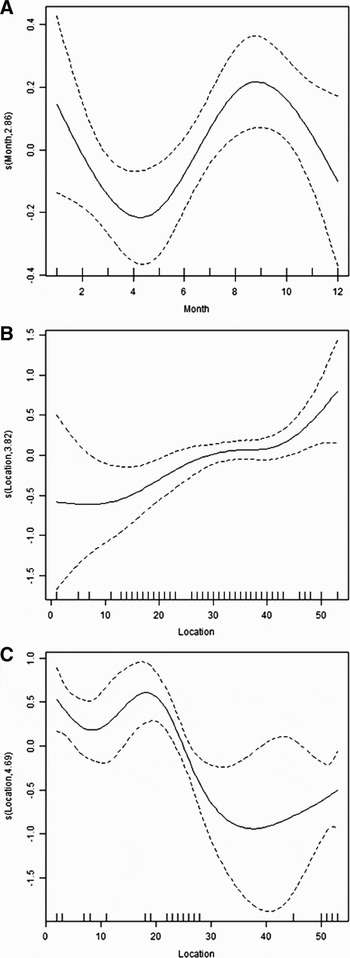
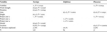
Generalized additive model results for numbers of cetaceans sighted, given presence, are summarized in Table 5. Numbers of bottlenose dolphins seen (given presence) were highest in January and September (Figure 4A), and higher numbers tended to be seen further south (Figure 4B). Smaller numbers were seen in the second project year than the first. Numbers seen were higher from higher observation points and when visibility was higher. Relationships with observation duration and wind strength, although significant, were non-linear and difficult to interpret: numbers seen were lowest for observation periods of around 40 minutes duration and increased for wind strengths from Beaufort 2 to Beaufort 4 (not illustrated). Of all these trends, only those for height, location and observation duration were strong (P < 0.01).
Smoothers for seasonal and spatial trends in numbers of cetaceans sighted, given presence. Effects of (A) month and (B) location on Tursiops numbers; (C) effect of location on Phocoena numbers.

Summary of generalized additive models for spatial and temporal patterns in numbers of animals seen, given presence, for Tursiops, Delphinus and Phocoena. For categorical explanatory variables, the effect given for each level is relative to a reference level (e.g. for number of observers, all comparisons are in relation to observation periods with one observer present). For each model, all significant explanatory variables are listed with their associated probability (P) value, along with the overall % deviance explained by the model and sample size (number of observation periods, N). For categorical and linear explanatory variables, the direction of the effect is indicated as + or –; for smoothers (s), the degrees of freedom are indicated in parentheses.

In the case of Delphinus delphis the only significant trends were for more animals to be seen where field of view area was larger and in the third and fourth project years compared to the first. Note that sample size was only around 1/3 of that for T. truncatus. In the case of P. phocoena, higher numbers were in the north (Figure 4C). More porpoises were seen in year 2 than in year 1. More porpoises were seen when visibility was higher and there was a weakly significant trend for fewer animals to be seen where field of view area was larger. Note that sample size was only around 1/7 of that for T. truncatus.
Environmental patterns in cetacean presence
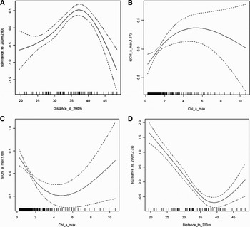
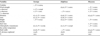
Generalized additive model results for cetacean presence in relation to environmental parameters are summarized in Table 6. In the final environmental model for T. truncatus presence there was a clear tendency for the species to be sighted most frequently where the shelf is between 35 and 40 km wide and in areas of higher maximum chl-a concentration (Figure 5A, B). Effects of observation duration and field of view area were highly significant, and Tursiops was seen more frequently from higher observation points and when 2 or 3 observers were present rather than one. Sightings were more frequent when visibility was higher (this trend was not significant in the previous analysis of spatiotemporal trends). The model explained 15.4% of deviance.
Smoothers for environmental models of Tursiops, Delphinus and Phocoena presence, showing effects of: (A) shelf width (distance from the coast to the 200 m isobath) and (B) maximum chlorophyll-a concentration on Tursiops presence, (C) the effect of maximum chlorophyll-a concentration on Delphinus presence and (D) shelf width on Phocoena presence.

Summary of generalized additive models for environmental patterns in presence of Tursiops, Delphinus and Phocoena. For categorical explanatory variables, the effect given for each level is relative to a reference level (e.g. for number of observers, all comparisons are in relation to observation periods with one observer present). For each model, all significant explanatory variables are listed with their associated probability (P) value, along with the overall % deviance explained by the model and sample size (number of observation periods, N). For categorical and linear explanatory variables, the direction of the effect is indicated as + or –; for smoothers (s), the degrees of freedom are indicated in parentheses.

Sightings of Delphinus delphis occurred most frequently where the continental shelf was narrowest (a linear trend) and more sightings occurred in areas with lower maximum chl-a concentrations (Figure 5C). Positive effects of increasing observation duration, field of view area and height of the observation point were evident at low values of these explanatory variables. The frequency of sightings was lowest around wind strength Beaufort 3–4 and was higher at both lower and higher wind strengths. There was a weak negative effect of having 3 observers rather than one. These trends are consistent with those in the spatiotemporal model for Delphinus presence.
The frequency of porpoise sightings was, similar to common dolphin sightings, negatively correlated with continental shelf width (Figure 5D) and maximum chlorophyll concentration. There were positive effects of longer observation duration (up to around 60 minutes) and presence of two or three observers rather than one and a negative relationship with both wind strength and height of the observation point. Porpoises were seen more frequently later in the day. Again these trends are consistent with the previous spatiotemporal model.
Environmental patterns in numbers of animals seen, given presence
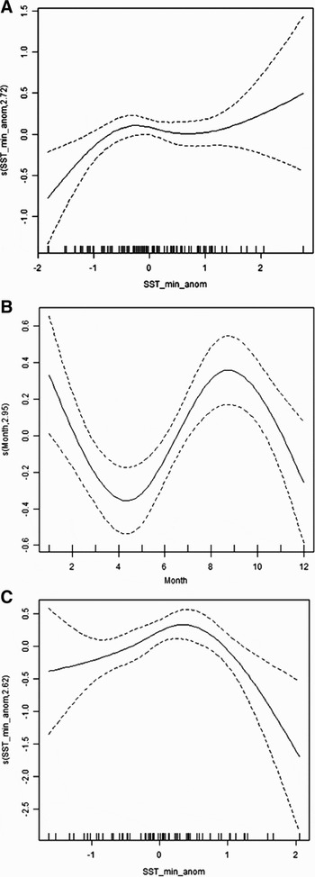
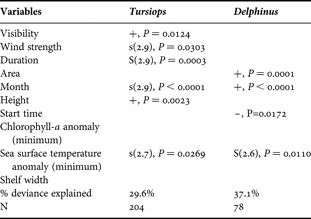
The numbers of T. truncatus seen, given presence, tended to be higher when minimum SST was slightly lower than the monthly average and, as evident in the previous spatiotemporal model of numbers of this species given presence, there was a clear peak in September (Table 7; Figure 6A, B). There were also positive effects of observation platform height, and visibility, again as seen for the spatiotemporal model of numbers given presence, non-linear effects of observation duration and wind strength.
Model for environmental trends in numbers of cetaceans sighted, given presence. Smoothers for effects of: (A) minimum sea surface temperature (SST) anomaly and (B) month on Tursiops numbers, and (C) effect of minimum SST anomaly on Delphinus numbers.

Summary of generalized additive models for environmental patterns in numbers seen, given presence, for Tursiops and Delphinus. For categorical explanatory variables, the effect given for each level is relative to a reference level (e.g. for number of observers, all comparisons are in relation to observation periods with one observer present). For each model, all significant explanatory variables are listed with their associated probability (P) value, along with the overall % deviance explained by the model and sample size (number of observation periods, N). For categorical and linear explanatory variables, the direction of the effect is indicated as + or –; for smoothers (s), the degrees of freedom are indicated in parentheses.

Numbers of Delphinus were highest later in the year (a trend not evident in the previous spatiotemporal model of numbers given presence) and where SST was slightly above its monthly mean value (Figure 6C). As for the previous spatiotemporal model of numbers given presence, numbers increased with field of view area (Table 7). No satisfactory environmental model could be fitted to the data on P. phocoena numbers.
Sampling efficiency
There were 267 sightings records for which T. truncatus was the only species seen and a further six for which this species was among two or more species sighted; the former subset was used for analysis. The modal waiting time at an observation site before a bottlenose dolphin was seen was around 10 minutes and majority of initial sightings of this species took place within 30 minutes of arrival at a site. There were 79 sightings records for which Delphinus delphis was the only species seen, plus 13 records for which this species was among two or more species sighted. The modal waiting time at an observation site before a common dolphin was seen was again around 10 minutes and most initial sightings took place within 60 minutes of arrival at a site. Phocoena phocoena was the only species seen on 32 occasions and it was one of two or more species seen on a further seven occasions. The modal waiting time to initial sighting was 10–15 minutes and most initial sightings took place within 35 minutes of arrival. This information suggests that site visits of 30 minutes duration may be adequate to record T. truncatus and P. phocoena but that Delphinus may be under-recorded if observation periods are less than 60 minutes.
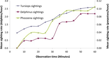
Based on the 1855 observation periods that lasted at least 30 minutes, average sightings rate of all three main species continues to increase with observation duration at least up to 30 minutes (not illustrated). There were 268 observation periods that lasted at least 1 hour (Figure 7). As expected given smaller sample sizes, the data are somewhat noisy but only the curve for T. truncatus shows any clear trend towards an asymptote.
Mean sightings rate versus observation time, based on all observations of at least 1 hour (N=268).

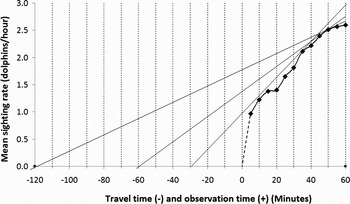
Applying the ‘optimal patch use’ analogy to the data on sightings rate achieved for T. truncatus, using data from observation periods of at least 1 hour, optimum waiting times are as little as 35 minutes if observers take 30 minutes to move between sites but rise to around 50 minutes for travel times of 1–2 hours (Figure 8). For the other species, since the sightings rate curves showed no indication of levelling off, it appears that optimal waiting times would be longer than for Tursiops.
‘Optimal waiting time’. Based on various possible travel times between observation sites, tangents are fitted to the sightings rate–observation time curve for Tursiops (based on data for 268 observation periods of at least 60 minutes duration) to indicate optimum waiting times in order to maximize sightings rate.

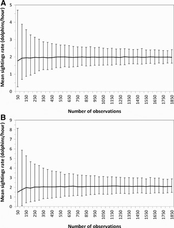
The total sample size for 30+ minute observations during the study period was 1855 observation periods. Figure 9 presents results from simulations based on these data, showing how mean sightings rate varies with sample size (number of observation periods) for 30 minute observation periods. While the average sightings rate stabilizes at fairly low sample sizes, there is a clear narrowing of confidence limits as sample size increases up to around 1000 observation periods.
Simulated mean sighting rates (animals/hour) as a function of the number of observation periods (50 to 1850), based on data from 1855 periods of at least 30 minutes: median and 95% confidence limits based on 1000 repeats per sample size/species combination: (A) Tursiops truncatus; (B) Delphinus delphis.

DISCUSSION
Which cetacean species are present, where and when?
The most frequently sighted cetacean species along the Galician coast was the bottlenose dolphin, seen almost three times as often as the next most common species, common dolphin, although total numbers of common dolphins seen were slightly larger, reflecting the larger group-sizes seen in the latter. These results presumably reflect the more coastal distribution of bottlenose dolphins, since common dolphins are thought to be more abundant overall in Galician waters, with four times as many common dolphins as bottlenose dolphins recorded from strandings and a ratio of 10:1 in sightings at sea (López et al., Reference López, Santos, Pierce, González, Valeiras and Guerra2002, Reference López, Pierce, Valeiras, Santos and Guerra2004).
The area with the highest overall frequency of cetacean sightings, and the highest frequency of bottlenose dolphin sightings, was between 42.5 and 43°N, around the Ría de Arosa and the Ría de Muros e Noia. This is consistent with the geographical distribution of strandings of T. truncatus along the coast as described by López et al. (Reference López, Santos, Pierce, González, Valeiras and Guerra2002) and at-sea sightings rate for this species reported by López et al. (Reference López, Pierce, Valeiras, Santos and Guerra2004). The probabilities of sightings of common dolphins and harbour porpoises showed peaks in three locations. Although differing somewhat between the two species, broadly speaking there were peaks in the north and south (around the borders with Asturias and Portugal respectively), and in the vicinity of Cabo Fisterre, the most westerly point of the Galician coast and somewhat to the north of the ‘hotspots’ for bottlenose dolphin occurrence. There is a rather striking inverse relationship between the overall frequencies of sightings of bottlenose dolphins and harbour porpoises along the coast (Figure 3).
The analysis additionally enabled quantification of some of the biases inherent in coastal observations, with effects of observation duration, field of view area, wind strength, visibility and number of observers all being demonstrated. Most of these trends were in the expected direction and it is important to note that they can be adequately controlled for in statistical analysis. Some trends were less intuitive. Thus higher observation sites tended to be associated with lower sightings rates for bottlenose dolphins and porpoises but higher sightings rate for common dolphins and larger group-sizes for bottlenose dolphins. Aside from possible effects of observation point height on the ease of seeing animals, it seems likely that the height of the observation site is providing information about the type of coastline and this requires further investigation.
In interpreting the sightings data it is important to keep in mind the behaviour of the animals seen adjacent to the coast. In all three of the most frequently seen species, groups were seen engaged in directional travel and non-directional movements, the latter including foraging boats. In porpoises, around 44% of groups observed undertook only non-directional movements, the figure being closer to 30% for the two dolphin species. All three species probably spend some time foraging close to the coast.
Habitat use
While all single species habitat models explained at least 20% of deviance, it should be borne in mind that some of this ‘explained’ variation is accounted for by the effects of variables related to observation effort and efficiency (e.g. wind strength and observation duration) so the explanatory power of the variables of interest, while statistically significant, is relatively low. In addition, the ‘environmental’ (habitat) models were generally somewhat weaker than the spatiotemporal models, as would be expected if not all the spatiotemporal variation in presence and numbers (as captured by effects of location, month and year) is related to variation in the suite of environmental variables available for modelling (namely continental shelf width and remotely sensed indices of SST and chlorophyll-a concentration).
The results of the habitat modelling suggested that bottlenose dolphin sightings are particularly associated with areas where the continental shelf is relatively wide and productivity (as indicated by remotely-sensed chlorophyll-a concentration in surface waters) relatively high. Presumably this is related to the abundance of their prey. Bottlenose dolphins in Galicia eat a wide range of fish species, the most important numerically and in terms of biomass being blue whiting (Micromesistius poutassou) and hake (Merluccius merluccius), which are also species of high commercial value. Blue whiting is probably taken at the shelf edge while hake can be taken on the shelf (Santos et al., Reference Santos, Fernández, López, Martínez and Pierce2007).
Common dolphins were seen most often where the continental shelf is narrowest and productivity lower, consistent with them normally occupying deeper waters. The most important prey in common dolphin diet in Galician waters are blue whiting and sardine (Sardina pilchardus) (Santos et al., Reference Santos, Pierce, López, Martínez, Fernández, Ieno, Mente, Porteiro, Carrera and Meixide2004). As is the case for bottlenose dolphins, common dolphins probably take blue whiting over the shelf break, while sardine is a more coastal species. Fishermen report common dolphins entering coastal waters to feed on sardine schools (M.B. Santos, personal communication).
Harbour porpoises also tended to be seen where the shelf is narrower, possibly indicating that they habitually occupy deeper waters. This is consistent with preliminary results from boat-based surveys, in which the average water depth for porpoise sightings was 90 m (CEMMA, unpublished data). Based on analysis of stomach contents of 32 porpoises stranded on the Galician coast during 1991–2004, the most important prey of harbour porpoise in Galician waters are scad (Trachurus trachurus), Trisopterus spp. and garfish (Belone belone). Blue whiting is the fourth most important species in the diet (Santos et al., unpublished data). While (as noted above) blue whiting is generally found on the continental slope, the other main prey species of porpoises species live in shelf waters.
Even though blue whiting are important in the diets of all three cetacean species, there are clearly also differences in the species of prey eaten and differences in habitat use would therefore not be surprising. Another factor to take into consideration is possible avoidance of competition and, in the case, of porpoises, avoidance attacks by bottlenose dolphins. Although bottlenose dolphin attacks on porpoises do not appear to be frequent in Galician waters, they have been documented (López & Rodriguez-Folgar, Reference López and Rodriguez Folgar1995; Alonso et al., Reference Alonso, López, González and Santos2000).
The sampling programme
To date the sampling regime has allowed observation duration to vary, mainly in the range 20–60 minutes, and the number of sites visited monthly was reduced from 53 to 30 from 2007. The present analysis allowed the efficiency of this sampling regime to be evaluated, based on the assumption that maximizing the sightings rate will provide the best information on species distribution. Clearly other criteria could have been used but this seems to be a reasonable starting point. It is evident from the data that sightings per unit effort (not only the absolute number of sightings) increased with observation duration. However, longer observation periods obviously impose additional resource requirements: since fewer sites can be visited in a day, more days of fieldwork are needed to complete the monthly circuit of all sites. Furthermore, estimated sightings rate will not increase indefinitely for longer observation periods. The raw data (Figure 7) provide some evidence of approach to an asymptote after 60 minutes in the case of bottlenose dolphins. GAM results (see Figure 3A) also suggest that there is a point of inflexion at around 40 minutes in the curve describing the increase in overall sightings rate for cetaceans in relation to observation duration. By analogy with optimal patch use (e.g. Charnov, Reference Charnov1976), once observer travel time between sites is taken into account, to maximize the sightings rate of bottlenose dolphins per hour of observer time, observation periods of 35–50 minutes appear be optimal. For the other cetacean species it is inevitable that longer observation periods would be needed to maximize sightings rates. Thus there is clear justification for observation periods in excess of 30 minutes.
Confidence limits for sightings rate appear to have stabilized after around 1000 observation periods. Almost 2500 observation periods were completed during 2003–2007, suggesting that there is scope for reducing the intensity of sampling. Thus the reduction in the number of sites visited from 53 to 30, made at the end of 2006 due to financial and logistic constraints, should not have greatly impacted on the value of the data collected for monitoring purposes.
The future
The Galician government is presently formulating Conservation Plans for both bottlenose dolphins and harbour porpoises. Survey data are needed to enable identification of areas that are consistently used by cetaceans, particularly feeding areas and areas frequented by females with calves. It will also be important to establish the seasonality of use of coastal waters. Results of the present study provide a clear indication that cetaceans are not evenly distributed along the coast, although the main species are present all year round.
Obviously, cetaceans range beyond coastal waters, and boat-based surveys are needed to fully document patterns and trends in cetacean distribution and habitat use. Nevertheless, the coastal sightings series has the potential to provide a relatively inexpensive long-term index of the status of local cetacean populations, which could be used to make inferences about the use of different areas of the coast by cetaceans, especially areas where no data are available from boat-based surveys, and to evaluate the impacts of threats such as climate change, overfishing, and pollution events.
Another focus for ongoing research will be evaluation of interactions with human activities, including fishing and boat traffic in general. While bottlenose dolphins can apparently become habituated to heavy boat traffic around ports (e.g. Sini et al., Reference Sini, Canning, Stockin and Pierce2005) this does not imply that boat traffic has no effect on the activity patterns and distribution, with many studies pointing to potentially harmful effects of disturbance by boats on bottlenose dolphins (e.g. Nowacek et al., Reference Nowacek, Wells and Solow2001; Hastie et al., Reference Hastie, Wilson, Tufft and Thompson2003; Mattson et al., Reference Mattson, Thomas and St Aubin2005; Bejder et al., Reference Bejder, Samuels, Whitehead, Gales, Mann, Connor, Heithaus, Watson-Capps, Flaherty and Krutzen2006). There is less evidence available on effects of disturbance on the other species of cetaceans known to inhabit Galician waters, although changes in activity due to disturbance by tourist boats have been detected elsewhere in both common dolphins and Risso's dolphins (Stockin et al., Reference Stockin, Lusseau, Binedell, Wiseman and Orams2008; Visser et al., Reference Visser, Hartman, Rood, Hendriks, Zult, Wolff, Huisman and Piercein press). The coastal sightings database provides one baseline data set against which to evaluate effects of, for example, future changes in the distribution and nature of tourism and fishing.
ACKNOWLEDGEMENTS
The authors wish thank all the volunteers and regional groups within CEMMA who contributed to the sightings surveys. The land-based sightings were funded by the Conselleria de Medio Ambiente e Desenvolvimento Sostenible, the Xunta de Galicia, Fundación Caixa Catalunhya and the Fundación Biodiversidad. G.J.P. was funded by the European Commission as part of the ANIMATE project (MEXC-CT-2006-042337). We also thank the referees for helpful suggestions about how to improve the manuscript.