1. Introduction
Turbulence arising from buoyant instabilities is a critical component in natural phenomena like underwater plumes, wildfire smoke and Type 1A supernovae. They also appear in engineering applications like inertial confinement fusion and scramjet combustors. A comprehensive list of examples can be found in the review article by Zhou (Reference Zhou2017a ). These instabilities occur when an interface between two fluids of unequal densities is subject to an acceleration, either impulsive or continuous.
Configurations related to RT with representative studies (#HD, number of homogeneous directions; USH, unstably stratified homogeneous turbulence).

Table 1. Long description
The table compares various RT-related configurations and studies, focusing on the number of homogeneous directions, statistical status, and sources of density variance. It has six rows and four columns. The columns are labeled Configuration, #HD, Stat., and Source of density variance. The rows are as follows: Row 1: Configuration, TRT (Cabot & Cook 2006); #HD, 2; Stat., No; Source of density variance, Pure fluid reservoirs. Row 2: Configuration, Livescu (Livescu & Ristorcelli 2008); #HD, 3; Stat., No; Source of density variance, Initial conditions. Row 3: Configuration, Chung (Chung & Pullin 2010); #HD, 2; Stat., Yes; Source of density variance, Source terms in fringe regions. Row 4: Configuration, Carroll (Carroll & Blanquart 2015); #HD, 3; Stat., Yes; Source of density variance, Numerical forcing terms. Row 5: Configuration, USH (Griffond et al. 2014); #HD, 3; Stat., No; Source of density variance, Physics-derived source terms. Row 6: Configuration, SRT (Goh & Blanquart 2025); #HD, 2; Stat., Yes; Source of density variance, Pure fluid reservoirs. Row 7: Configuration, HBT; #HD, 3; Stat., Yes; Source of density variance, Physics-derived source terms.
Cases where the applied acceleration is continuous are referred to as Rayleigh–Taylor (RT) instabilities. They were originally investigated by Rayleigh (Reference Rayleigh1882) and Taylor (Reference Taylor1950) as a linear stability problem. When the acceleration field is directed from the heavy fluid to the light, baroclinic torque causes disturbances in the interface to grow exponentially until nonlinear effects become dominant and a turbulent layer forms. Experimental (Dimonte & Schneider Reference Dimonte and Schneider2000; Ramaprabhu & Andrews Reference Ramaprabhu and Andrews2004; Banerjee, Kraft & Andrews Reference Banerjee, Kraft and Andrews2010) and computational (Youngs Reference Youngs1984; Zhou Reference Zhou2001; Ristorcelli & Clark Reference Ristorcelli and Clark2004; Vladimirova & Chertkov Reference Vladimirova and Chertkov2009; Youngs Reference Youngs2013) studies of the turbulent layer have found an asymptotic tendency towards self-similar growth. In this limit, the height of the layer
 $h$
evolves according to a differential equation of the form
 \begin{equation} \dot {h}^2 \propto h \end{equation}
where a variety of definitions have been used for
 $h$
(a list is given in table 1 of Goh & Blanquart (Reference Goh and Blanquart2025)). The integral length scale scales with
 $h$
and the turbulent velocity scales with
 $\dot {h}$
. While the height of the layer grows, the Kolmogorov length scale
 $\eta$
,
 \begin{equation} \eta = \left ( \frac {\nu ^3}{\widetilde {\epsilon }} \right )^{1/4}, \end{equation}
where
 $\nu$
is the kinematic viscosity and
 $\widetilde {\epsilon }$
is the Favre average of viscous dissipation, shrinks, such that the Reynolds number rises over time.
A review of RT research in general is given by Zhou (Reference Zhou2017a , Reference Zhoub ). More specialized reviews in theoretical modelling (Abarzhi Reference Abarzhi2010), the Boussinesq limit (Boffetta & Mazzino Reference Boffetta and Mazzino2017) and experiments (Andrews & Dalziel Reference Andrews and Dalziel2010; Banerjee Reference Banerjee2020) also exist. Schilling (Reference Schilling2020) provides a summary of efforts to integrate models, simulations and experiments.
1.1. Computational challenges
Practical RT flows are characterized by high Reynolds numbers, often combined with shocks, combustion and multiphase interactions. These complications make direct numerical simulations (DNS) prohibitively expensive to resolve. Large-eddy simulations (LES) could reduce the necessary resolution to a tractable level, but they require subgrid scale (SGS) models that accurately represent the unresolved turbulence. Unfortunately, only a few RT LES studies have used explicit SGS models (Mellado, Sarkar & Zhou Reference Mellado, Sarkar and Zhou2005; Burton Reference Burton2009; Yilmaz Reference Yilmaz2020; Luo et al. Reference Luo, Wang, Yuan, Jiang, Huang and Wang2023); the others have relied on implicit LES (Dimonte et al. (Reference Dimonte2004) and references therein) or artificial fluid models (Cook, Cabot & Miller Reference Cook, Cabot and Miller2004). Among the SGS studies, only a few (Cook et al. Reference Cook, Cabot and Miller2004; Luo et al. Reference Luo, Wang, Yuan, Jiang, Huang and Wang2023) have made attempts to validate against DNS results. Moreover, LES studies of related flows, such as buoyant plumes (Tieszen et al. Reference Tieszen, O’Hern, Schefer, Weckman and Blanchat2002; DesJardin, O’Hern & Tieszen Reference Desjardin, O’Hern and Tieszen2004) and buoyant wall-jets (Addad, Benhamadouche & Laurence Reference Addad, Benhamadouche and Laurence2004) have had difficulty predicting root-mean-square (r.m.s.) velocity and achieving grid independence. Novel SGS models, designed specifically to account for buoyant effects, are necessary before RT LES becomes reliable.
Performing DNS on the canonical planar RT configuration is one way to investigate the physics of RT instabilities without relying on intractable resolutions or unproven SGS models. In this configuration, hereafter referred to as temporally evolving Rayleigh–Taylor (TRT), the acceleration is constant, the domain is rectangular and the fluids are initially separated into two semi-infinite, uniform, quiescent reservoirs,
 \begin{gather} \rho (t=0,x_i) = \left \{ \begin{array}{ll} \rho _L, & x_1 \lt 0, \\[3pt] \rho _H, & x_1 \gt 0, \end{array} \right . \end{gather}
 \begin{gather} u_i(t=0, x_i) = 0, \end{gather}
where
 $\rho$
is the density,
 $u_i$
is the velocity and the
 $H$
and
 $L$
subscripts indicate properties of the heavy and light fluids. The flow can be characterized by three non-dimensional numbers: a Reynolds number,
 \begin{equation} {\textit{Re}} = \frac {\dot {h} h}{\nu }; \end{equation}
an Atwood number,
 \begin{equation} {\textit{At}} = \frac {\rho _H - \rho _L}{\rho _H + \rho _L}; \end{equation}
a Schmidt number,
 \begin{equation} {\textit{Sc}} = \frac {\nu }{D}. \end{equation}
Here,
 $\nu$
is kinematic viscosity, and
 $D$
is the scalar diffusivity. Some of the largest TRT DNS to date include the studies of Cabot & Cook (Reference Cabot and Cook2006) (
 $3 072^3$
grid points) and Livescu, Wei & Petersen (Reference Livescu, Wei and Petersen2011) (
 $4096^2\times 4032$
grid points).
Though inexpensive compared with practical RT configurations, TRT suffers from computational drawbacks.
-
(i) Long simulation time. For a given target Reynolds number, the TRT must be run from the initial perturbations until the layer grows to the necessary height. This means that the bulk of the computational cost is spent on simulating a flow that is less turbulent than the regime of interest.
-
(ii) Growing domain size. Because the height of the RT layer grows with time, the final Reynolds number sets the required domain size for the overall simulation. Therefore, either the entire simulation must be run with the final computational grid, or the grid must evolve with time. The former approach over-resolves the flow at early times, and the latter approach introduces the non-trivial cost and complexity of an adaptive grid.
-
(iii) Statistical non-stationarity and inhomogeneity. Since the flow and its statistics evolve with time, the flow at the exact desired Reynolds number can only be observed over a short time window. Because the flow is homogeneous in only the two horizontal directions, an estimate of an ensemble average statistic can only be calculated from a single plane of grid points. Further data must be gathered from additional realizations, each requiring a new simulation starting from initial perturbations.
1.2. Alternative configurations
To circumvent one or more of the computational inefficiencies associated with TRT, alternative configurations have been proposed to capture the same physics at a reduced cost.
Livescu & Ristorcelli (Reference Livescu and Ristorcelli2007) initialized random blobs of heavy and light fluid in a triply periodic box domain, then applied a constant gravitational field. This produced buoyancy-generated turbulence that is homogeneous in all three directions, allowing easier estimation of statistics. However, the turbulence still evolves continuously until the two fluids mix completely and the turbulence decays.
Chung & Pullin (Reference Chung and Pullin2010) also used a triply periodic box with the same initialization, but added source and sink terms of density, active in fringe regions at the top and bottom (respectively) of the domain. These serve to counteract the turbulence decay in a manner analogous to fluid reservoirs, inducing a stationary buoyant flow. Averages can be taken over time, but not in the vertical spatial direction, which is inhomogeneous. The resulting flow is sensitive to the form of the source terms over much of the domain, so that relevant results are limited to a narrow slab around the horizontal midplane.
Carroll & Blanquart (Reference Carroll and Blanquart2015) used a source term (active throughout the domain) to maintain the density variance in a triply periodic box. This source term is active everywhere, so that the flow is both stationary and homogeneous in all three directions. However, the term itself has no physical justification; it is questionable whether the generated density fluctuations are representative of real fluctuations in RT layers.
Griffond, Gréa & Soulard (Reference Griffond, Gréa and Soulard2014) proposed another forced homogeneous scheme called unstably stratified homogeneous turbulence. Here, the governing equations have some physical justification, being a modified form of the Boussinesq equations for stably stratified turbulence (Godeferd & Cambon Reference Godeferd and Cambon1994). However, the framework assumes small density perturbations (
 ${At \approx 0}$
). Furthermore, the flow fails to achieve stationarity, increasing in Reynolds number indefinitely.
Goh & Blanquart (Reference Goh and Blanquart2025) recently introduced a configuration called stationary Rayleigh–Taylor (SRT). In this framework, the TRT boundary conditions and fluid reservoirs are present, but the coordinates and velocity are rescaled to account for temporal evolution in the self-similar limit. The result resembles a statistically stationary version of the TRT configuration. The domain no longer grows with time, but homogeneity is still limited to two directions and a significant portion of the computational grid is still taken up by the reservoirs. The full SRT equations are reviewed in § 2.2.
1.3. Homogeneous buoyant turbulence
The properties of each of the discussed frameworks are summarized in table 1. All have succeeded in creating flows with some combination of three-dimensional homogeneity, stationarity and sources of density variance representative of TRT, but not all three at once.
To this end, the authors propose a novel configuration called homogeneous buoyant turbulence (HBT). The inspiration for this configuration is taken from the procedure of Rah, Dhandapani & Blanquart (Reference Rah, Dhandapani and Blanquart2018). By adapting the reasoning used by Lundgren (Reference Lundgren2003) to derive his linear forcing term for homogeneous isotropic turbulence (HIT), Rah et al. (Reference Rah, Dhandapani and Blanquart2018) isolated and modelled the small scales of turbulence at the centreline of a round incompressible jet. They began by defining a set of transformations of the flow variables to homogenize them at a specific location along the centreline. After substitution in the Navier–Stokes equations, evaluation at the target location and simplifications guided by an analysis of the kinetic energy budget, the authors obtained a new set of governing equations, identical to the original except for source terms in the momentum equations. When implemented in a triply periodic box domain, these source terms act to maintain the kinetic energy. The resulting stationary homogeneous flow was found to reproduce statistics (including turbulence spectra) observed in DNS of turbulent round jets. The same procedure was later applied to shear layers (Dhandapani, Rah & Blanquart Reference Dhandapani, Rah and Blanquart2019).
The objective of the present study is to use the same procedure to model the small scales of turbulence near the midplane of an RT instability. The result is a statistically stationary, fully homogeneous simulation framework for studying RT instabilities.
The paper is arranged thus: § 2 describes the derivation of the HBT governing equations, analogous to Rah et al. (Reference Rah, Dhandapani and Blanquart2018). Section 3 discusses the closure of these equations and the non-dimensionalization of the simulation parameters. Section 4 describes the computational methods and lists the simulation cases. Sections 5 and 6 present the results, first a series of low-Reynolds number cases to elucidate numerical properties of the framework, then a few high Reynolds number cases to validate results against the TRT DNS performed by Cabot & Cook (Reference Cabot and Cook2006). Finally, § 7 summarizes the computational benefits afforded by HBT and briefly addresses potential applications to turbulence model development.
2. Governing equations
The governing equations for HBT are derived in five steps. In § 2.1, the TRT governing equations are introduced. In § 2.2, variable transformations are substituted into the governing equations to achieve statistical stationarity. In § 2.3 further transformations are applied to approximate statistical homogeneity at the layer midplane. In § 2.4, these transformations are substituted into the stationary governing equations to derive a new set of equations. Finally, negligible terms are removed to produce the HBT governing equations in § 2.5.
Throughout the following discussion, an overline indicates a Reynolds (ensemble) average,
 $\overline {\phi }$
, and a tilde indicates a Favre average,
 $\widetilde {\phi } = \overline {\rho \phi }/ \overline {\rho }$
. A prime and double prime indicate the corresponding fluctuations:
 $\phi ' = \phi - \overline {\phi }$
,
 $\phi '' = \phi - \widetilde {\phi }$
.
2.1. Governing equations for TRT
The canonical RT configuration is governed by the low-Mach number, variable-density, Navier–Stokes equations with a single transported scalar,
 \begin{align} \frac {\partial {\rho }}{\partial t} + \frac {\partial {\rho u_{\!j}}}{\partial x_{\!j}} &= 0, \\[-12pt]\nonumber \end{align}
 \begin{align} \frac {\partial {\rho u_i}}{\partial t} + \frac {\partial {\rho u_i u_{\!j}}}{\partial x_{\!j}} &= -\frac {\partial {p}}{\partial x_i} + \frac {\partial {\tau _{ij}}}{\partial x_{\!j}} - (\rho - \overline {\rho }) g \delta _{1i}, \\[-12pt]\nonumber \end{align}
 \begin{align} \frac {\partial {\rho Y}}{\partial t} + \frac {\partial {\rho u_{\!j} Y}}{\partial x_{\!j}} &= \frac {\partial {}}{\partial x_{\!j}}\left (\rho D \frac {\partial {Y}}{\partial x_{\!j}}\right )\!, \end{align}
where
 $\rho$
is the density,
 $u_i$
is the
 $i$
th component of velocity,
 $p$
is the pressure,
 $Y$
is the scalar,
 $D$
is the diffusivity,
 $g$
is the gravity and
 $\tau _{ij}$
is the viscous stress tensor, defined as
 \begin{equation} \tau _{ij} = \rho \nu \left ( \frac {\partial {u_i}}{\partial x_{\!j}} + \frac {\partial {u_{\!j}}}{\partial x_i} - \frac {2}{3}\frac {\partial {u_k}}{\partial x_k} \delta _{ij} \right )\!, \end{equation}
where
 $\nu$
is the kinematic viscosity (assumed constant for this study) and
 $\delta _{ij}$
is the Kronecker delta. Einstein summation notation is used for the coordinate indices. Here, the hydrostatic component of the gravity,
 $-\overline {\rho } g \delta _{1i}$
, has been absorbed into the pressure gradient, such that the pressure is uniform within each reservoir.
The four flow variables,
 $u_i$
,
 $\rho$
,
 $p$
and
 $Y$
, are determined by (2.1)–(2.3) and an equation of state (EoS) of the form
 \begin{equation} \rho = f(Y). \end{equation}
In the TRT configuration, the ideal gas EoS is used,
 \begin{equation} \rho = \frac {P_o W}{\textit{RT}}, \end{equation}
where
 $P_o$
is the spatially uniform background pressure,
 $W$
is the mixture molecular weight and
 $R$
is the universal gas constant. It is further assumed that variations in density can arise from either the molar mass
 $1/W = Y/W_{\!L} + (1-Y)/W_{\!H}$
or the temperature
 $T = \textit{YT}_L + (1-Y) T_H$
, but not both. The scalar
 $Y$
represents either the mass fraction of the lighter fluid in a binary mixture or a non-dimensionalized temperature. In either case, the EoS can be written as
 \begin{equation} \rho = \frac {1}{\alpha Y + \beta } \end{equation}
where
 $\alpha$
and
 $\beta$
are constant coefficients that can be chosen arbitrarily, provided the initial and boundary conditions of
 $Y$
are consistent with those of
 $\rho$
. For example, when the density is bounded between two limits,
 $\rho _L$
and
 $\rho _H$
, it is common to set
 $\alpha =1/\rho _L + 1/\rho _H$
and
 $\beta = -1/\rho _H$
such that
 $0\leqslant Y \leqslant 1$
. However, it is more algebraically convenient in the context of this study to set
 $\beta =0$
so that
 \begin{equation} \rho = \frac {1}{\alpha Y}, \end{equation}
and
 $1/(\alpha \rho _H) \leqslant Y \leqslant 1/(\alpha \rho _L)$
. Here
 $\alpha$
can also be set to a value of
 $1$
for convenience, but it is retained symbolically in the analysis for dimensional consistency.
The canonical RT configuration initializes these equations with two reservoirs of heavy/light fluid separated by a disturbed planar interface. This produces a flow that is statistically homogeneous and isotropic in the two horizontal directions, but neither homogeneous nor isotropic vertically. The height of the resulting mixing layer grows indefinitely, so that statistical stationarity is never achieved.
2.2. Variable transformations for stationarity
Recently, Goh & Blanquart (Reference Goh and Blanquart2025) proposed a modification to the TRT governing equations to simulate the RT instability in a statistically stationary framework. Their work relies on a rescaling of the variables according to the expected growth of velocity scales and length scales in the self-similar limit:
 \begin{gather} t^{\dagger }=t, \quad x_1^{\dagger } = \frac {h_0}{h(t)} x_1, \quad x_2^{\dagger } = x_2, \quad x_3^{\dagger } = x_3, \end{gather}
 \begin{gather} \rho ^{\dagger } = \rho , \quad u^{\dagger }_i = u_i \frac {\dot {h}_0}{\dot {h}(t)}, \quad Y^{\dagger } = Y, \quad \frac {\partial {p^{\dagger }}}{\partial x_i^{\dagger }} = \frac {\partial {p}}{\partial x_i}, \end{gather}
where
 $h$
is any measure of the mixing height, and
 $h_o$
is its value at an arbitrary time
 $t=t_o$
. Although the horizontal coordinates scale with the layer height as well, they are not rescaled in the transformations to preserve horizontal homogeneity. In SRT, this causes horizontal length scales to grow until confined by the periodic boundary conditions. Nonetheless, the successful validation of SRT against TRT by Goh & Blanquart (Reference Goh and Blanquart2025) indicates that the confined horizontal scales behave analogously to a rescaling of the TRT horizontal scales.
The full form of the governing (2.1)–(2.3) with the substitutions of (2.9) and (2.10) are given in Goh & Blanquart (Reference Goh and Blanquart2025). They are omitted here for brevity. The full rescaled equations are still not stationary, since the Reynolds number will continue to increase as the Kolmogorov length scales shrink. To induce stationarity, Goh & Blanquart (Reference Goh and Blanquart2025) introduces the following three assumptions:
-
(i) the governing equations evaluated at
 $h(t) = h(t_0)$
are valid for a window of time centred at
$t=t_0$
and longer than the integral time scale;
-
(ii) within this window, ensemble-averaged quantities are approximately constant, i.e.
$\partial (\overline {\boldsymbol{\cdot }}) /\partial t^\dagger \approx 0$
; -
(iii) within this window,
$h(t)$
exhibits self-similar growth, as in (1.1).


With these assumptions, the equations simplify to
 \begin{align} \frac {\partial {\rho ^{\dagger }}}{\partial t} + \frac {\partial {\rho ^{\dagger } u_{\!j}^{\dagger }}}{\partial x_{\!j}^{\dagger }} &= R_\rho , \\[-12pt]\nonumber \end{align}
 \begin{align} \frac {\partial {\rho ^{\dagger } u_i^{\dagger }}}{\partial t^{\dagger }} + \frac {\partial {\rho ^{\dagger } u_i^{\dagger } u_{\!j}^{\dagger }}}{\partial x_{\!j}^{\dagger }} &= -\frac {\partial {p^{\dagger }}}{\partial x_i^{\dagger }} + \frac {\partial {\tau _{ij}^{\dagger }}}{\partial x_{\!j}^{\dagger }} - (\rho ^{\dagger } - \overline {\rho ^{\dagger }}) g \delta _{1i} + T_u + R_{u_i}, \\[-12pt]\nonumber \end{align}
 \begin{align} \frac {\partial {\rho ^{\dagger } Y^{\dagger }}}{\partial t} + \frac {\partial {\rho ^{\dagger } u_{\!j}^{\dagger } Y^{\dagger }}}{\partial x_{\!j}^{\dagger }} &= \frac {\partial {}}{\partial x_{\!j}^{\dagger }}\left (\rho ^{\dagger } D \frac {\partial {Y^{\dagger }}}{\partial x_{\!j}^{\dagger }}\right ) + R_Y, \end{align}
where
 \begin{equation} \tau _o = \frac {h(t_o)}{\dot {h}(t_o)} \end{equation}
is the instantaneous time scale of the self-similar growth,
 \begin{align} R_\rho = \frac {x_1^{\dagger }}{\tau _o} \frac {\partial {\rho ^{\dagger }}}{\partial x_1^{\dagger }}, \quad R_{u_i} = \frac {x_1^{\dagger }}{\tau _o} \frac {\partial {\rho ^{\dagger } u_i^{\dagger }}}{\partial x_1^{\dagger }}, \quad R_Y =\frac {x_1^{\dagger }}{\tau _o} \frac {\partial {\rho ^{\dagger } Y^{\dagger }}}{\partial x_1^{\dagger }} \end{align}
are source terms associated with the vertical length rescaling, and
 \begin{equation} T_{u_i} = - \frac {1}{2 \tau _o}\rho ^{\dagger } u_i^{\dagger } \end{equation}
is a source term associated with the velocity rescaling. The coordinate system is chosen such that
 $x_1^{\dagger } = 0$
corresponds to the midplane, the location about which the self-similar growth occurs. This coincides with the location of the initial interface between the fluid reservoirs and the location where
 $\partial (\overline {\rho ^{\dagger } u_1^{\dagger }})/\partial x_1^{\dagger } = 0$
.
Throughout the study, SRT data from Goh & Blanquart (Reference Goh and Blanquart2025) will be referenced as cases G1–G6, and SRT data from Goh et al. (Reference Goh, Matehuala and Blanquart2026) will be referenced as cases A01, A2, A5 and A8. Their corresponding Atwood number and midplane statistics are given in table 2. These statistics include the turbulent Reynolds number
 \begin{equation} {\textit{Re}_t} = \frac {\widetilde {k}^2}{\widetilde {\epsilon } \nu }, \end{equation}
where
 $k=u_i^2/2$
is the kinetic energy and
 $\epsilon = \tau _{ij} (\partial u_i / \partial x_{\!j})$
is the viscous dissipation, and an effective local Atwood number
 \begin{equation} {\textit{At}_{\textit{eff}}} = \frac {\overline {\rho ^{\prime 2}}^{1/2}}{\overline {\rho }}. \end{equation}
The relationship between
 ${\textit{At}_{\textit{eff}}}|_{x_1=0}$
and
 ${\textit{At}}$
in TRT can be inferred from SRT data. Figure 1(a,b) shows
 ${\textit{At}_{\textit{eff}}}|_{x_1=0}$
plotted against both
 ${\textit{Re}_t|_{x_1=0}}$
and
 ${\textit{At}}$
for SRT cases. Here
 ${\textit{At}_{\textit{eff}}}|_{x_1=0}$
is nearly constant with respect to Reynolds number and almost linear with
 ${\textit{At}}$
. Therefore
 ${\textit{At}_{\textit{eff}}}|_{x_1=0}$
is a valid one-to-one metric for
 ${\textit{At}}$
.
List of SRT simulation cases from Goh & Blanquart (Reference Goh and Blanquart2025) and Goh et al. (Reference Goh, Matehuala and Blanquart2026). Output parameters are evaluated at midplane. For all cases,
 ${Sc = 1}$
.

Table 2. Long description
A table with 10 rows and 4 columns. The columns are labeled Case, Re_t, At, and At_eff. The table lists various simulation cases with their corresponding turbulent Reynolds number (Re_t), Atwood number (At), and effective local Atwood number (At_eff). Row 1: Case, G1; Re_t, 50; At, 0.5; At_eff, 0.27. Row 2: Case, G2; Re_t, 130; At, 0.5; At_eff, 0.25. Row 3: Case, G3; Re_t, 240; At, 0.5; At_eff, 0.24. Row 4: Case, G4; Re_t, 350; At, 0.5; At_eff, 0.23. Row 5: Case, G5; Re_t, 990; At, 0.5; At_eff, 0.23. Row 6: Case, G6; Re_t, 1880; At, 0.5; At_eff, 0.23. Row 7: Case, A01; Re_t, 360; At, 0.01; At_eff, 0.004. Row 8: Case, A2; Re_t, 370; At, 0.2; At_eff, 0.09. Row 9: Case, A5; Re_t, 360; At, 0.5; At_eff, 0.24. Row 10: Case, A8; Re_t, 290; At, 0.8; At_eff, 0.44.
Midplane values of
 ${\textit{At}_{\textit{eff}}} = \rho _{\textit{rms}}/\overline{\rho }$
versus (a)
 ${\textit{Re}_t}$
at the midplane for cases G1–6 of Goh & Blanquart (Reference Goh and Blanquart2025), with horizontal line indicating mean value, and (b)
 ${\textit{At}}= (\rho _H - \rho _L)/(\rho _H + \rho _L)$
for cases {A01, A2, A5, A8} of Goh et al. (Reference Goh, Matehuala and Blanquart2026), with linear fit.

2.3. Variable transformations for homogeneity
The aim of the proposed framework is the simultaneous satisfaction of statistical homogeneity in horizontal directions, homogeneity in the vertical direction and stationarity in time. The original equations (see § 2.1) are horizontally homogeneous; the transformations and simplifications of § 2.2 introduce stationarity. A second variable transformation,
 \begin{equation} \rho ^{\dagger }, u_i^{\dagger }, p^{\dagger } \rightarrow \rho ^*, u_i^*, p^*, \end{equation}
is now sought to introduce vertical homogeneity.
The transformations of (2.19) only contain sufficient degrees of freedom to make three statistics exactly uniform while maintaining the form of the EoS. The statistics chosen are
 $\overline {\rho ^*}$
,
 $\overline {\rho ^* u_1^*}$
and
 $\overline {p^*}$
, leading to the transformations
 \begin{gather} \rho ^{*} = \rho ^{\dagger } \frac {\overline {\rho ^{\dagger }_o}}{\overline {\rho ^{\dagger }}}, \quad u^{*}_i = (u_i^{\dagger } - \widetilde {u_1^{\dagger }} \delta _{1i}) \left (\frac {\overline {\rho ^{\dagger }}}{\overline {\rho ^{\dagger }_o}} \right )^{1/2}, \quad p^* = p^\dagger - \overline {p^\dagger }, \quad Y^* = \frac {\overline {\rho ^\dagger }}{\overline {\rho _o^\dagger }} Y^\dagger. \end{gather}
The `o’ subscript implies evaluation at the midplane. Here
 $\overline {\rho ^*}$
is homogenized by normalizing
 $\rho ^\dagger$
by its ensemble average, while
 $\overline {\rho ^* u_1^*} = \overline {\rho ^*} \widetilde {u_1^*}$
and
 $\overline {p^*}$
are homogenized by subtracting the corresponding mean values from
 $u_i^\dagger$
and
 $p^\dagger$
. The transformation for
 $Y^*$
is defined to maintain the form of the EoS.
Averages over time and horizontal coordinates from SRT data (case G4). The vertical coordinate is normalized by the layer height as defined by Goh & Blanquart (Reference Goh and Blanquart2025), and statistics are normalized by their midplane values. The orange and purple shaded areas represent the regions where
 $\overline {\rho ^* u_2^{*2}}$
and
 $\overline {Y^{*'2}}$
are within 5 % of their midplane values, respectively.

Although the transformations (2.20) homogenize exactly only three statistics, they induce approximate uniformity in a number of other statistics in the region surrounding the midplane. This is illustrated in figure 2. For the G4 SRT case, four statistics of the transformed variables are shown across the vertical coordinate:
 $\overline {\rho ^* u_1^{*2}}$
,
 $\overline {\rho ^* u_2^{*2}}$
,
 $\overline {Y^*}$
and
 $\overline {Y^{*'2}}$
. The first three of these remains within
 $5\,\%$
of their respective midplane value over a region of length
 $\approx 0.3 h_m$
centred at the midplane, where
 $h_m$
is the definition of the layer height used by Goh & Blanquart (Reference Goh and Blanquart2025),
 \begin{equation} h_m = \frac {4(\rho _H + \rho _L)}{\rho _H \rho _L} \int \langle \rho Y (1-Y) \rangle _{2\text{-D}} \mathrm{d} x_1, \end{equation}
and
 $\langle \boldsymbol{\cdot }\rangle _{2D}$
indicates a horizontal planar average. Note that the bounds of this region of homogeneity may not hold at higher Atwood number (i.e. greater than 0.5), where the peaks of these and other statistics shift towards the light fluid side of the layer (Goh et al. Reference Goh, Matehuala and Blanquart2026). This effect is already apparent at
 ${\textit{At}}=0.5$
in the
 $\overline {Y^{*'2}}$
profile of figure 2. Though more than
 $0.34h_m$
in width, the centre of its region of homogeneity is shifted to the left of the midplane by
 $\approx 0.08 h_m$
.
Table 3 gives values for the minimum distance
 $H$
from the midplane where each statistic is greater than
 $5\,\%$
from its midplane value, multiplied by
 $2$
. This represents the maximum width of a region centred on the midplane where the statistic can be said to be homogeneous. Thus, HBT can be expected to model accurately TRT length scales at or below this metric.
Size of homogeneity region about the midplane for statistics in the G4 SRT case, as measured by the minimum distance
 $H$
from the midplane where a statistic deviates by more than
 $5\,\%$
from its midplane value.

Table 3. Long description
A table comparing statistics for two different cases in the G4 SRT scenario. The table has three rows and three columns. The columns are labeled Statistic, 2H/h_m, and 2H/l_1†. The rows are labeled with different statistics and their corresponding values. Row 1: ρ*u_1*^2, 0.41, 0.24. Row 2: ρ*u_2*^2, 0.28, 0.17. Row 3: Y^+, 1.61, 0.96. Row 4: Y^+*^2, 0.20, 0.12.
The distances are normalized by both
 $h_m$
and the characteristic vertical length scale
 $l_1^\dagger$
. The latter is defined in terms of the vertical longitudinal correlation length,
 \begin{align} l_1^\dagger = 2\pi \varLambda ^\dagger _1 = 2\pi \int C_1^\dagger (r) \mathrm{d}r, \quad C_1^\dagger (r) = \frac {\left \langle {u^\dagger _1}' (t^\dagger ,x_1^\dagger +r, x_2^\dagger , x_3^\dagger ) {u^\dagger _1}'(t,x_1^\dagger , x_2^\dagger , x_3^\dagger )\right \rangle _{2\text{-D}}}{\left \langle {u^\dagger _1}'^2 \right \rangle _{2\text{-D}}}, \end{align}
previously used by Zhou & Cabot (Reference Zhou and Cabot2019) for analysis of TRT and Goh & Blanquart (Reference Goh and Blanquart2025) for analysis of SRT. While the homogeneous region of
 $\overline {Y^*}$
spans more than one layer height and nearly one
 $l_1^\dagger$
, the others only span a fraction of
 $h_m$
and less than 20 % of
 $l_1^\dagger$
. These regions may become even smaller at higher
 ${\textit{At}}$
as the profiles shift downwards. Nonetheless,
 $\kappa \geqslant 2\pi /0.12 l_1$
represents a sizable portion of the turbulence length scales, and
 ${At \leqslant 0.5}$
accounts for most RT problems of practical relevance. Moreover, the quantitative comparison in § 6.3 will show that the turbulence spectra of HBT reproduce TRT spectra at scales well above the limits indicated by table 3.
While homogeneity is satisfied either exactly or approximately for several key statistics, some statistics remain inhomogeneous even at low Atwood number. These include the turbulent flux of kinetic energy
 $\overline {\rho ^* u^*_1 u_i^{*2}}$
, the pressure flux of kinetic energy
 $\overline {u_1^* p^*}$
and the turbulent flux of scalar variance
 $\overline {u^{*'}_1 Y^{*'2}}$
. Unfortunately, the degrees of freedom afforded by the variable transformations do not permit the homogenization of these fluxes. This is accepted as an inevitable source of error in the formulation. The impact of these inhomogeneities on the kinetic energy and scalar variance budgets are addressed in § 2.5.
2.4. Source terms
From the transformations proposed in the previous section, the inverse transformations can be obtained:
 \begin{gather} \rho ^\dagger = \frac {\overline {\rho ^\dagger }}{\overline {\rho ^\dagger _o}} \rho ^*, \quad u_i^\dagger = \left ( \frac {\overline {\rho ^\dagger _o}}{\overline {\rho ^\dagger }} \right )^{1/2} u_i^* + \widetilde {u^\dagger _1} \delta _{1i}, \quad p^\dagger =p^* + \overline {p^\dagger }, \quad Y^\dagger = \frac {\overline {\rho ^\dagger _o}}{\overline {\rho ^\dagger }} Y^*. \end{gather}
These transformations are now substituted into the governing equations for SRT. In the subsequent discussion, all variables not marked with an asterisk are presumed to carry the dagger superscript, which is omitted to save space.
At the same time, we leverage the exact and approximate homogeneity induced by the transformations to apply the following assumption:
-
(i) for a horizontal slab centred vertically at
$x_1=0$
, ensemble-averaged quantities of starred variables are approximately uniform, i.e.
$\partial (\overline {\boldsymbol{\cdot }})/\partial x_1 \approx 0$
.


We also introduce the following two assumptions, which simplify the final equations:
-
(ii) within this slab, the governing equations evaluated at
$\overline {\rho }(x_1) = \overline {\rho }(0)$
,
$\overline {\rho u}_1(x_1) = \overline {\rho u}_1(0)$
,
$( {\mathrm{d}{\overline {\rho }}}/{\mathrm{d} x_1})(x_1) = ({\mathrm{d}{\overline {\rho }}}/{\mathrm{d} x_1})(0)$
and
$({\mathrm{d}{\overline {\rho u_1}}}/{\mathrm{d} x_1})(x_1) =( {\mathrm{d}{\overline {\rho u_1}}}/{\mathrm{d} x_1})(0) = 0$
are valid; -
(iii) within this slab,
$R_\rho$
,
$R_{u_i}$
and
$R_Y$
source terms arising from the stationarity transformations, being proportional to
$x_1$
, are negligible.


Starting with continuity (2.11),
 \begin{equation} \frac {\partial {}}{\partial t} \left ( \frac {\overline {\rho }}{\overline {\rho }_o} \rho ^* \right ) + \frac {\partial {}}{\partial x_{\!j}} \left \{ \left [ \frac {\overline {\rho }}{\overline {\rho }_o} \rho ^* \right ] \left [ \left ( \frac {\overline {\rho }_o}{\overline {\rho }} \right )^{1/2} u_{\!j}^* + \widetilde {u}_1 \delta _{1j} \right ] \right \} = R_\rho . \end{equation}
Applying assumption (iii) and rearranging gives
 \begin{equation} \frac {\partial {}}{\partial t} \left ( \frac {\overline {\rho }}{\overline {\rho }_o} \rho ^* \right ) + \frac {\partial {}}{\partial x_{\!j}} \left [ \left (\frac {\overline {\rho }}{\overline {\rho }_o} \right )^{1/2} \rho ^* u_{\!j}^* \right ] + \frac {\partial {}}{\partial x_1} \left (\frac {\overline {\rho }}{\overline {\rho }_o} \rho ^* \widetilde {u}_1 \right ) = 0. \end{equation}
This is then expanded to yield
 \begin{equation} \frac {\rho ^*}{\overline {\rho }_o} \frac {\partial {\overline {\rho }}}{\partial t} + \frac {\overline {\rho }}{\overline {\rho }_o} \frac {\partial { \rho ^*}}{\partial t} + \left (\frac {\overline {\rho }}{\overline {\rho }_o} \right )^{1/2} \left ( \frac {\partial {\rho ^* u_{\!j}^*}}{\partial x_{\!j}} +\frac {1}{2 \overline {\rho }} \frac {\partial {\overline {\rho }}}{\partial x_1} \rho ^* u_1^*\right ) + \frac {\overline {\rho }}{\overline {\rho }_o} \left ( \widetilde {u}_1 \frac {\partial {\rho ^* }}{\partial x_1} + \frac {\rho ^*}{\overline {\rho }} \frac {\partial {\overline {\rho }\widetilde {u}_1}}{\partial x_1} \right ) = 0. \end{equation}
Leveraging statistical stationarity and applying assumption (ii) leads to
 \begin{equation} \frac {\partial { \rho ^*}}{\partial t} + \widetilde {u}_{1o} \frac {\partial {\rho ^* }}{\partial x_1}+ \frac {\partial {\rho ^* u_{\!j}^*}}{\partial x_{\!j}} + \frac {1}{2 \overline {\rho }_o} \frac {\mathrm{d}{\overline {\rho }}}{\mathrm{d} x_1} \bigg |_{x_1=0} \rho ^* u_1^* = 0. \end{equation}
Performing a Galilean frame shift where
 $ ({{\rm D}}/{{\rm D} t}) = ({\partial }/{\partial t})+ \widetilde {u}_{1o} ( {\partial }/{\partial x_1})$
further simplifies the equation. By assumption (i), the starred variables are statistically homogeneous, so this frame shift has no effect on the flow statistics. The transformed continuity equation is then
 \begin{equation} \frac {{\rm D}{\rho ^*}}{{\rm D} t} + \frac {\partial {\rho ^* u_{\!j}^*}}{\partial x_{\!j}} = S_\rho , \end{equation}
which contains the additional source term
 \begin{equation} S_\rho = - \frac {\rho ^* u_{1}^*}{2\lambda _o} \end{equation}
where
 \begin{equation} \lambda _o = \left (\frac {1}{\overline {\rho }_o} \frac {\mathrm{d}{\overline {\rho }}}{\mathrm{d} x_1} \bigg |_{x_1=0}\right )^{-1} \end{equation}
is a characteristic length scale associated with the density variation and mixing layer height.
To disentangle the evolution of density from that of the other primitive flow variables, the momentum (2.12) is first rewritten in its advective form, and assumption (iii) is applied to remove
 $R_{u_i}$
:
 \begin{align} \frac {\partial {u_i}}{\partial t} + u_{\!j} \frac {\partial {u_i}}{\partial x_{\!j}} &= \frac {1}{\rho } \left ( -\frac {\partial {p}}{\partial x_i} + \frac {\partial {\tau _{ij}}}{\partial x_{\!j}} + g (\rho - \overline {\rho }) \delta _{i1} - \frac {1}{2 \tau _o}\rho u_i \right )\!. \end{align}
Following a similar procedure as for the continuity equation, the momentum equation becomes
 \begin{equation} \frac {{\rm D}u_i^*}{{\rm D}t} + u_{\!j}^* \frac {\partial {u_i^*}}{\partial x_{\!j}} = \frac {1}{\rho } \left ( -\frac {\partial {p^*}}{\partial x_i} + \frac {\partial {\tau _{ij}^*}}{\partial x_{\!j}} + g (\rho ^* - \overline {\rho ^*}) \delta _{i1} - \frac {1}{2 \tau _o}\rho ^* u_i^* \right ) + S_{u_i} \end{equation}
and the source term is
 \begin{align} S_{u_i} = - \frac {1}{\rho ^*}\frac {\mathrm{d}{\overline {p}}}{\mathrm{d} x_1} +\frac {1}{\rho ^*}\frac {\partial {\tau _{ij} - \tau _{ij}^*}}{\partial x_{\!j}} - \frac {\widetilde {u}_1}{2 \tau _o}\delta _{1i} + \frac {1}{\lambda _o}\left [ \frac {u_1^* u^*_i}{2} + \frac {\widetilde {u}_1 u^*_i }{2} + \left ( \widetilde {u}_1 u_1^* + \widetilde {u}_1^2 \right ) \delta _{1i} \right ] \end{align}
where
 $\tau _{ij}^*$
is defined in the same way as its unstarred counterpart
 $\tau _{ij}$
in (2.4) but with the corresponding transformed flow variables.
Finally, the scalar equation transforms to
 \begin{equation} \frac {{\rm D} Y^* }{{\rm D} t} + u_{\!j}^* \frac {\partial {Y^*}}{\partial x_{\!j}} = \frac {1}{\rho ^*}\frac {\partial {}}{\partial x_{\!j}} \left ({\rm D} \rho ^* \frac {\partial {Y^*}}{\partial x_{\!j}} \right ) + S_Y \end{equation}
with the source term
 \begin{equation} S_Y = - {\rm D} Y^*\frac {\partial {}}{\partial x_{\!j}} \left ( \frac {1}{\overline {\rho }} \frac {\partial {\overline {\rho }}}{\partial x_1} \right ) + \frac {1}{\lambda _o} \left ( u_1^* Y^* + \widetilde {u}_1 Y^* \right ). \end{equation}
To be used in the present numerical framework, the advective (2.32) and (2.34) must be converted back to conservative form,
 \begin{align} \frac { {\rm D}\rho ^* u_i^*}{{\rm D}t} + \frac {\partial {\rho ^* u_{\!j}^* u^*_i}}{\partial x_{\!j}}& = - \frac {\partial {p^*}}{\partial x_i} + \frac {\partial {\tau _{ij}^*}}{\partial x_{\!j}} + g\rho ^{*'} \delta _{i1} - \frac {1}{2 \tau _o}\rho ^* u^*_i + \rho ^* S_{u_i} + u_i^* S_\rho, \\[-12pt]\nonumber \end{align}
 \begin{align} \frac {{\rm D} \rho ^* Y^* }{{\rm D} t} + \frac {\partial { \rho ^* u_{\!j}^* Y^*}}{\partial x_{\!j}} &=\frac {\partial {}}{\partial x_{\!j}} \left ( {\rm D} \rho ^* \frac {\partial {Y^*}}{\partial x_{\!j}} \right ) + \rho ^* S_Y + Y^* S_\rho, \end{align}
where
 $S_\rho$
has entered through application of continuity (2.28).
While (2.28) and (2.36) are independent of the EoS, the EoS enters into the derivation of (2.37) twice. First, the transformation
 $Y \rightarrow Y^*$
in (2.20) is defined in terms of the general EoS,
 $\rho =f(Y)$
, as
 \begin{equation} Y^* = f^{-1}\left ( \frac {\overline {\rho }_o}{\overline {\rho }} f(Y) \right )\!. \end{equation}
Second, after the transformations (2.20) are substituted into the original transport equation, the EoS is used to simplify the resulting equation to (2.37). The source terms that appear in the final transformed equation cannot be predicted universally, and can only be derived for a given EoS by defining the function
 $f(Y)$
and repeating the full derivation.
2.5. Simplifications
Equations (2.28), (2.36) and (2.37), with the EoS (2.8), govern the transformed flow variables near the midplane in SRT. Interestingly, many of the source terms added by the transformation have a relatively small impact on the flow and can be neglected. In this section, numerical SRT data will be surveyed across
 ${\textit{Re}}$
and
 ${\textit{At}}$
parameter space to determine which terms may be neglected.
The most obvious metric to assess the relative magnitude of each source term is the first moment of each equation. However, by definition of the transformed variables, the first moment of every term in the continuity equation is already zero. Similarly, the mean momentum and mean scalar equations do not provide much insight. Since reproducing the turbulent dynamics of the fluctuations is the intent of the present work, we compare scalings and magnitudes of the second moments.
For the transformed continuity equation, we compare the following five r.m.s. quantities:
 \begin{align} C_{i} &= \overline {\left ( \frac {\partial {\rho ^* u_i^*}}{\partial x_i} \right )^2}^{1/2} \forall \, i \in \{ 1,2,3 \}, & C_4&=\overline {\left ( \sum _{j=1}^3\frac {\partial {\rho ^* u_{\!j}^*}}{\partial x_{\!j}} \right )^2}^{1/2}, & C_5 &= \frac {1}{2 \lambda _o} \overline { \left ( \rho ^* u_1^* \right ) ^2}^{1/2}, \end{align}
where there is no sum on the
 $i$
indices. Here
 $C_1, C_2$
and
 $C_3$
represent the r.m.s. of the transformed convective terms individually,
 $C_4$
the r.m.s. of the same terms summed together and
 $C_5$
the r.m.s. of the source term
 $S_\rho$
. We include
 $C_4$
because the fluctuations of the individual derivatives in the convective term cancel to produce smaller fluctuations in the total divergence of
 $\rho ^* u_i^*$
. Since the first moment of each term is zero, the relative magnitude of
 $C_5$
represents the influence of the source term over the continuity relationship and the flow overall.
Quantities of (2.39), evaluated at midplane in SRT, plotted against (a) turbulent Reynolds number for cases G1–4 of Goh & Blanquart (Reference Goh and Blanquart2025) and (b) Atwood number for cases {A0, A2, A5, A8} of (Goh et al. Reference Goh, Matehuala and Blanquart2026), normalized by
 $C_1$
. Where
 $i$
takes more than one value, the quantity is the average of the components with the corresponding indices.

Figure 3 shows each quantity, normalized by
 $C_1$
, measured at the midplane for SRT cases G1–4. Since they are statistically equivalent,
 $C_2$
and
 $C_3$
are averaged together. For each case,
 $C_5$
is significantly smaller than the other r.m.s. values. Its ratio with
 $C_1$
decreases approximately as
 ${\textit{Re}_t^{-1/2}}$
, a scaling predicted by the self-similarity analysis of Ristorcelli & Clark (Reference Ristorcelli and Clark2004), and increases linearly with
 ${\textit{At}}$
. Since
 $C_5$
is an order of magnitude less than all other terms for
 ${\textit{Re}_t}\gt 200$
, and scales with
 ${\textit{At}}$
in the same way as the next smallest term,
 $C_4$
, the assumption that
 $S_\rho$
is negligible in (2.28) is understood to be valid for
 ${\textit{Re}_t}\geqslant 200$
and all
 ${\textit{At}} \leqslant 0.8$
. All RT flows of practical relevance fall in this regime.
To assess the momentum terms, the second moment of the conservative form of the momentum equation is used. The equation for kinetic energy
 $\overline {\rho ^*} \widetilde {k^*} = \overline {\rho ^*} \widetilde {u^{*2}_i}/2$
is obtained by multiplying the momentum (2.36) by
 $u^{*}$
and applying continuity:
 \begin{align} \frac { D \overline {\rho ^*} \widetilde {k^*}}{D t} = \underbrace {- \frac {\partial {\dfrac {1}{2} \overline {\rho ^*} \widetilde {u_i^{* 2} u_{\!j}^* }}}{\partial x_{\!j}} - \frac {\partial {\overline {u_i^* p^* }}}{\partial x_i}}_{I} \underbrace {+ \overline {p^* \frac {\partial {u_i^* }}{\partial x_i}}}_{\textit{II}} \underbrace {- \overline {\rho ^*} \widetilde {\epsilon ^*} }_{\textit{III}} \underbrace { + \frac {\partial {\overline {u_i^* \tau _{ij}^* }}}{\partial x_{\!j}}}_{\textit{IV}} \underbrace {+ g \overline {\rho ^{*'} u_1^{*'} }}_{V} \underbrace {- \frac {1}{2 \tau _o} \overline {\rho ^*} \widetilde {u_i^{*2}}}_{\textit{VI}} + \nonumber \\ \overline {\rho ^* u_i^* S_{u_i}} + \frac {1}{2} \overline {u_i^{*2} S_\rho }. \end{align}
Using the definitions from (2.29) and (2.33), the source terms become
 \begin{equation} \overline {\rho ^* u_i^* S_{u_i}} + \frac {1}{2} \overline {u_i^{*2} S_\rho } = \underbrace {- \overline {u^*_1}\frac {\mathrm{d}{\overline {p}}}{\mathrm{d} x_1}}_{\textit{VII}} \underbrace {+ \overline {u_i^* \frac {\partial {\tau _{ij} - \tau _{ij}^*}}{\partial x_{\!j}}}}_{\textit{VIII}} \underbrace {+ \frac {\widetilde {u}_1 \overline {\rho ^*} \widetilde {k^*} }{\lambda _o}}_{\textit{IX}} \underbrace {+ \frac {\widetilde {u}_1 \overline {\rho ^*} \widetilde {u_1^{*2}}}{\lambda _o}}_{X} \underbrace {+ \frac { \overline {\rho ^*} \widetilde {u^*_1 u_i^{*2}}}{4 \lambda _o}}_{\textit{XI}}. \end{equation}
The terms of (2.40), evaluated at the midplane of SRT cases and normalized by buoyant production, are presented in figure 4(a) for varying
 ${\textit{Re}_t}$
. As mentioned earlier, the kinetic energy is not strictly homogeneous at the midplane, so the advective term within the material derivative (left-hand side) is not exactly zero. However, it is consistently less than 1 % of the buoyant production. Similarly, the pressure dilatation (II) and two source terms (IV and VIII) represent less than 1 % of the production term. These are omitted from figure 4(a,b) and are understood to be negligible. All remaining terms show little variation in Reynolds number. Figure 4(b) shows the midplane values of the kinetic energy budget terms at varying
 ${\textit{At}}$
. The dissipation, buoyant production and layer growth (terms III, V and VI) remain in nearly constant proportion at all
 ${\textit{At}}$
. Transport (I) decreases gradually with
 ${\textit{At}}$
, but not according to any apparent power law. The magnitudes of terms IX, X and XI increase from zero as
 ${\textit{At}}$
rises.
Term VII remains below 2 % of the buoyant production at all tested
 ${\textit{Re}_t}$
and
 ${\textit{At}}$
and is therefore neglected. While terms IX and XI reach 10 % of production for the highest Atwood case, they are less than 5 % of production across Reynolds number for
 ${\textit{At}} \leqslant 0.5$
. Furthermore, their magnitudes are similar and of opposite signs across the parameter space; their contributions are expected to cancel. Thus, terms IX and XI are also neglected.
The dominant balance of the kinetic energy budget is between buoyant production (V), viscous dissipation (III), layer growth (VI), turbulent and pressure transport (I) and, at high
 ${\textit{At}}$
, the source term X. The transport term arises directly from inhomogeneity in the transformed turbulent flux of kinetic energy
 $\overline {\rho u_1^* u_i^{*2}}$
and the transformed pressure flux
 $\overline {u_1^* p^*}$
. As discussed in § 2.3, this inhomogeneity is a consequence of the limited degrees of freedom available in defining the variable transformations (2.20). It is apparent from figure 4(a) that the increase in the magnitude of term X is nearly balanced by a decrease in the transport, so that summed together, these terms have a nearly constant contribution across
 ${\textit{Re}_t}$
and
 ${\textit{At}}$
. As a modelling closure, the buoyant production in HBT is reduced to account for the energy sink that these terms would otherwise provide. The implementation of this reduction is discussed further in § 3.1.
Terms in the transformed kinetic energy budget (2.40) evaluated at midplane versus (a) turbulent Reynolds number for cases G1–4 of Goh & Blanquart (Reference Goh and Blanquart2025) and (b) Atwood number for cases {A01, A2, A5, A8} of (Goh et al. Reference Goh, Matehuala and Blanquart2026). Values are normalized by the term of largest magnitude. Terms with normalized absolute values consistently below 0.01 are omitted. The inset shows the same data in greater detail near the x-axis.

Figure 4. Long description
Two line graphs depict the evaluation of terms in the transformed kinetic energy budget at midplane versus turbulent Reynolds number and Atwood number. Panel A: A line graph shows the relationship between various terms in the transformed kinetic energy budget and the turbulent Reynolds number. The x-axis is labeled with the turbulent Reynolds number, and the y-axis is labeled with the term over V. The graph includes multiple lines, each representing a different term, with labels I, III, V, VI, VII, IX, X, and XI. The inset shows the same data in greater detail near the x-axis. Panel B: Another line graph shows the relationship between the same terms and the Atwood number. The x-axis is labeled with the Atwood number, and the y-axis is labeled with the term over V. The graph also includes multiple lines, each representing a different term, with the same labels as in Panel A. The values are normalized by the term of largest magnitude, and terms with normalized absolute values consistently below 0.01 are omitted.
The scalar variance transport equation is derived by multiplying the advective form (2.34) of the scalar equation by
 $Y^{*'}$
, then ensemble averaging,
 \begin{align} \frac { D \overline {Y^{ *'2}}}{\textit{Dt}} =& \underbrace {- \overline {u_1^*} \frac {\partial {\overline {Y^{ *'2}}}}{\partial x_1}}_{I} \underbrace {-\frac {\partial {\overline { u_1^{*'} Y^{ *'2}}}}{\partial x_1}}_{\textit{II}} \underbrace {+ 2\overline {u_1^{*'} Y^{*'}} \frac {\partial {\overline {Y^*}}}{\partial x_1}}_{\textit{III}} \nonumber \\ &\qquad \underbrace {- 2 \overline {\chi } }_{\textit{IV}} \underbrace {+ D \frac {\partial 2 \overline {Y^{ *'2}}}{\partial x_1^2}}_{V} \underbrace {+ 2 D \overline {Y^{* '} \left ( \frac {1}{\rho ^* } \frac {\partial {\rho ^* }}{\partial x_{\!j}} \frac {\partial {Y^*}}{\partial x_{\!j}} \right ) }}_{\textit{VI}} + 2 \overline {Y^{ *'} S_Y} \end{align}
where the scalar dissipation rate is
 \begin{equation} \chi = D \left (\frac {\partial {Y^{ *'}}}{\partial x_{\!j}} \right )^2 \!. \end{equation}
With the definition from (2.35), the source terms become
 \begin{equation} 2 \overline {Y^{ *'} S_Y} = \underbrace {- 2 D \overline {Y^{*'2}}\frac {\partial {}}{\partial x_{\!j}} \left ( \frac {1}{\overline {\rho }} \frac {\partial {\overline {\rho }}}{\partial x_1} \right )}_{\textit{VII}} \underbrace {+ 2 \frac {( \overline {u_1^*} + \widetilde {u}_1) \overline {Y^{*'2}} }{\lambda _o}}_{\textit{VIII}} \underbrace {+ 2 \frac { \overline {u_1^{*'} Y^{*'}Y^{*}}}{\lambda _o}}_{\textit{IX}}. \end{equation}
The terms of the scalar variance budget are computed at the midplane of SRT and presented in figure 5(a) at varying
 ${\textit{Re}_t}$
. They are normalized by the mean gradient production. As in the kinetic energy equation, while the scalar variance is not strictly homogeneous at the midplane, the advective term in the material derivative is negligible (
 $\lt 1\,\%$
of the production term). Similarly, terms I, V, VII and VIII are each less than
 $1\,\%$
of production and are omitted from the figure. The remaining terms are insensitive to Reynolds number. Figure 5(b) gives the midplane scalar variance budget terms at varying Atwood. The relative contributions of terms III and VI increase from zero as
 ${\textit{At}}$
rises. Notably, the decrease in the magnitude of term IV appears to balance the increase in term VI, while the decrease in term II is balanced by the increase in term III.
Terms in the transformed scalar variance budget (2.42) evaluated at midplane versus (a) turbulent Reynolds number for cases G1–4 of Goh & Blanquart (Reference Goh and Blanquart2025) and (b) Atwood number for cases {A0, A2, A5, A8} of (Goh et al. Reference Goh, Matehuala and Blanquart2026). Values are normalized by the term of largest magnitude. Terms with normalized absolute values consistently below 0.01 are omitted. The inset shows the same data in greater detail near the x-axis.

The dominant balance is between the mean gradient production (XI), scalar dissipation (IV), turbulent transport (II) and a diffusive term arising from variation in density (VI), as well as the source term III at high Atwood. Like the pressure transport and turbulent transport of kinetic energy, the contribution to scalar variance by turbulent transport is a consequence of inhomogeneity in the transformed variables. The sum of terms II and III constitutes a variance sink that is nearly uniform across the parameter space, which is modelled in HBT by a reduction in the mean gradient production term, as discussed in § 3.1.
From the above analysis, the only term within the sources
 $S_\rho$
,
 $S_{u_i}$
and
 $S_Y$
with a non-negligible contribution to continuity, kinetic energy transport or scalar variance transport is term IX in (2.44). The source terms therefore become
 \begin{align} S_\rho \approx 0, \quad S_{u_i} \approx 0, \quad S_Y \approx \frac {u^{*'}_1 Y^*}{\lambda _o}. \end{align}
Substituting these into the transformed governing (2.28) and (2.36)–(2.37), the equations for HBT are now given by
 \begin{equation} \frac {\partial {\rho ^*}}{\partial t} + \frac {\partial {\rho ^* u_{\!j}^*}}{\partial x_{\!j}} = 0, \end{equation}
 \begin{equation} \frac {\partial {\rho ^* u_i^*}}{\partial t} + \frac {\partial {\rho ^* u_i^* u_{\!j}^*}}{\partial x_{\!j}} = -\frac {\partial {p^*}}{\partial x_i} + \frac {\partial {\tau _{ij}^*}}{\partial x_{\!j}} + g \rho ^{*'} \delta _{1i} - \frac {1}{2 \tau _o}\rho ^* u_i^*, \end{equation}
 \begin{equation} \frac {\partial {\rho ^* Y^*}}{\partial t} + \frac {\partial {\rho ^* Y^* u_{\!j}^*}}{\partial x_{\!j}} = \frac {\partial {}}{\partial x_{\!j}}\left (\rho ^* D \frac {\partial {Y^*}}{\partial x_{\!j}}\right ) + \frac {u_1^{*'}}{\alpha \lambda _o}, \end{equation}
where the source term in the scalar equation has been simplified using the EoS (2.8). The mean gradient source term on the right-hand side of (2.48) acts to maintain the scalar variance, which in turn acts through the buoyancy term in (2.47) to maintain the kinetic energy.
It is interesting to note that (2.48) has the same form as the transport equation for temperature fluctuations in Rayleigh–Benard convection, where a mean temperature gradient is imposed. Seeing as the horizontally averaged scalar profile in an RT layer is approximately linear at the midplane, and inertial range scalings at the core of an RT mixing layer have been observed to be equivalent to those of Rayleigh–Benard convection in the two-dimensional (2-D) Boussinesq case (Mazzino Reference Mazzino2017), it is not surprising that analogous flow dynamics emerge. The inclusion of
 $- (1/2 \tau _o)\rho ^* u_i^*$
in (2.47) to represent self-similar growth distinguishes HBT, a statistically stationary representation of a non-stationary flow, from Rayleigh–Benard convection, a statistically stationary flow.
3. Flow inputs for HBT
Aside from the initial and boundary conditions, running a simulation with the governing equations (2.46)–(2.48) requires knowledge of five parameters:
 $\nu$
,
 $D$
,
 $g$
,
 $\tau _o$
and
 $\lambda _o$
. Constant values can be prescribed to
 $\nu$
and
 $D$
as inputs. Sections 3.1 and 3.2 describe how the remaining variables are determined. Section 3.3 shows how non-dimensional groupings corresponding to the TRT non-dimensional parameters arise from the simulation inputs.
3.1. Layer growth term
Measurements of
 $\tau _t/\tau _o$
at midplane for SRT and TRT cases, versus the turbulent Reynolds number at midplane. Ensemble averages are approximated by averages across horizontal directions and, for SRT cases, time.

The momentum equations in the HBT formulation (2.47) inherit one coefficient from the SRT formulation, the time scale
 $\tau _o$
. In the formulation of Goh & Blanquart (Reference Goh and Blanquart2025), it was identified with the inverse of the global average scalar dissipation rate over the entire mixing layer. Obviously, such a closure expression could not be extended to the HBT formulation. Nonetheless, other time scales are available in HBT which scale in the same manner as
 $\tau _o$
.
Since
 $\tau _o$
appears in the turbulent kinetic energy budget, and the goal of HBT is to reproduce the turbulence dynamics of SRT, it would be advantageous to relate
 $\tau _o$
to a time scale associated with the kinetic energy budget. The time scale chosen is the midplane value of the turbulence time scale
 $\tau _t = \widetilde {k}_o/\widetilde {\epsilon }_o$
.
As established in § 2.2,
 $\tau _o$
models
 $h/\dot {h}$
in the corresponding TRT simulation. According to the scalings derived by Ristorcelli & Clark (Reference Ristorcelli and Clark2004),
 $h/\dot {h}$
scales with
 ${\textit{Re}}$
and
 ${\textit{At}}$
in the same way as
 $\tau _t$
in the self-similar limit. Therefore,
 $\tau _t$
and
 $\tau _o$
can be related to each other by a single non-dimensional constant across all values of
 ${\textit{Re}}$
and
 ${\textit{At}}$
. To evaluate this constant,
 $\tau _t/\tau _o$
is measured over SRT cases G1–6 of Goh & Blanquart (Reference Goh and Blanquart2025). In figure 6, these measurements are plotted against the turbulent Reynolds number at the midplane. The TRT case T0 of Goh & Blanquart (Reference Goh and Blanquart2025) and the TRT data of Cabot & Cook (Reference Cabot and Cook2006) are also shown for comparison, where
 $h_m/\dot {h}_m$
is used in place of
 $\tau _o$
. The SRT values appear to be constant across Reynolds number, confirming that
 $\tau _t$
and
 $\tau _o$
scale with
 ${\textit{Re}_t}$
in the same way. The six cases are averaged to yield
 $\tau _t/\tau _o \approx 0.41$
. This average lies largely between the two TRT series, within 20 % of most of the data. In the HBT framework, the time scale
 $\tau _o$
is replaced by
 $\tau _t/0.41$
. To compute
 $\tau _t$
numerically, the volume averages of turbulent kinetic energy and viscous dissipation rate are taken at each time step.
It is also noted that
 $ \tau _t / \tau _o = (\widetilde {k^*} / \tau _o)/ \widetilde {\epsilon ^*}$
, i.e. the ratio of the turbulence time scale and the layer growth time scale is equal to the ratio of the layer growth and viscous contributions to the kinetic energy budget (terms VI and III in (2.40)). Since the HBT budget is dominated by the buoyant production, viscous dissipation and layer growth, fixing the ratio between the latter two implies that any deviation in the balance of the HBT budget from TRT can be reduced to error in the magnitude of the production term. Thus, the terms neglected in § 2.5, such as the pressure and turbulent transport, emerge in HBT as a reduction in buoyant production. Likewise, since the scalar variance budget in HBT is dominated by just two terms, the neglected scalar variance budget terms emerge as a reduction in the mean gradient production.
3.2. Temporal fluctuation reduction
The ability of (2.46)–(2.48) to produce turbulence in a homogeneous setting relies upon the presence of two source terms in the vertical velocity and scalar equations,
 \begin{align} f_g = g \rho ^{*'}, \quad f_\lambda = \frac {u^{*'}_1}{\alpha \lambda _o}, \end{align}
representing the effects of gravity and the mean density gradient, respectively. Other source terms have been used to sustain HBT in previous studies (Soulard, Griffond & Gréa Reference Soulard, Griffond and Gréa2014; Carroll & Blanquart Reference Carroll and Blanquart2015). Unfortunately, like many homogeneous forcing methods (Eswaran & Pope Reference Eswaran and Pope1988; Overholt & Pope Reference Overholt and Pope1998; Carroll & Blanquart Reference Carroll and Blanquart2013), these source terms produce statistics subject to large temporal fluctuations and correlations over long time scales. As a result, simulations must be run over long times to obtain time-averaged statistics within an acceptable degree of uncertainty. Shortening the required simulation time requires reducing either the correlation time scale or the fluctuation magnitude. While some stochastic forcing schemes (Eswaran & Pope Reference Eswaran and Pope1988) permit the adjustment of the correlation time as an input parameter, it is undesirable to introduce stochasticity into a forcing term that is representative of a deterministic physical process. In the present work, measures are taken to reduce the temporal fluctuations instead.
Large, correlated fluctuations have also been identified (Carroll & Blanquart Reference Carroll and Blanquart2013) as a difficulty in the implementation of Lundgren (Reference Lundgren2003)’s linear forcing term,
 \begin{equation} f_L = A u_i, \end{equation}
where
 $A$
is a constant forcing coefficient. The term appears in the momentum equation in the context of constant density turbulence:
 \begin{equation} \frac {\partial {u_i}}{\partial t} + u_{\!j} \frac {\partial {u_i}}{\partial x_{\!j}} = - \frac {\partial {p}}{\partial x_i} + \nu \frac {\partial 2 u_i}{\partial x_{\!j}^2} + f_L. \end{equation}
If this equation is multiplied by
 $u_i$
, the Reynolds average is taken and homogeneity is assumed, the kinetic energy equation is obtained as
 \begin{equation} \frac {\partial {\overline {k}}}{\partial t}= -\overline {\epsilon } + 2A \overline {k}. \end{equation}
If stationarity is further assumed, the following relationship results:
 \begin{equation} 2A = \frac {\overline {\epsilon }}{\overline {k}} = \frac {1}{\tau _t}. \end{equation}
The forcing effectively induces the turbulence time scale
 $\tau _t$
time to approach
 $1/2A$
as the flow relaxes towards stationarity.
Initially proposed by Rosales & Meneveau (Reference Rosales2005), Carroll & Blanquart (Reference Carroll and Blanquart2013) explored the effects of a modification to the Lundgren forcing:
 \begin{equation} f_L^* = A\frac {k_o}{\langle k \rangle } u_i. \end{equation}
Here
 $k_o$
is another constant, and the angle brackets indicate a volume-averaged quantity, which is a function of time only. The relationship of (3.5) becomes instead
 \begin{equation} 2A k_o = \overline {\epsilon } \end{equation}
so that the forcing coefficient determines the value of
 $\overline {\epsilon }$
rather than
 $\tau _t$
. In other words,
 $2 A k_o$
represents a prescribed constant rate of kinetic energy injection, which
 $\overline {\epsilon }$
must balance to maintain a stationary state.
Carroll & Blanquart (Reference Carroll and Blanquart2013) demonstrated that the modified source term (3.6) produces smaller fluctuations in
 $\langle {k}\rangle$
and
 $\langle \epsilon \rangle$
than the original source term (3.5). This was supported theoretically by a linear perturbation analysis, which suggests that the Lundgren forcing is only marginally stable for fluctuations in
 $\langle {k}\rangle$
and
 $\langle \epsilon \rangle$
, whereas the modified Lundgren scheme damps the same fluctuations to smaller amplitudes.
To produce a similar effect, an analogous modification is proposed for the HBT forcing terms of (3.1). If the pressure dilatation is neglected, the kinetic energy equation for the HBT momentum (2.47) becomes
 \begin{equation} \frac {\partial {\overline {\rho ^*}\widetilde {k^*}}}{\partial t} = -1.41\overline {\rho ^*} \widetilde {\epsilon ^*} + g \overline {\rho ^{*'} u^{*'}_1}. \end{equation}
Stationarity then implies
 \begin{equation} g = -1.41\frac {\overline {\rho ^*} \widetilde {\epsilon ^*}}{ \overline {\rho ^{*'} u^{*'}_1}} \end{equation}
so that prescribing a value for
 $g$
is equivalent to imposing the ratio of the viscous dissipation and the density–vertical velocity covariance. Likewise, the scalar variance equation becomes
 \begin{equation} \frac {\partial {\overline {\rho ^*}\widetilde {Y^{*''2}}}}{\partial t} = -\overline {\rho ^*} \widetilde {\chi ^*} + \frac { \overline {u^{*'}_1 Y^{*'}}}{\alpha \lambda _o}. \end{equation}
At stationarity this is
 \begin{equation} \frac { 1}{\alpha \lambda _o}= \frac {\overline {\rho ^*} \widetilde {\chi ^*}}{\overline {u^{*'}_1 Y^{*'}}}. \end{equation}
The ratio of the scalar dissipation and the vertical velocity-scalar covariance is imposed.
We propose to modify the original source terms (3.1) as follows:
 \begin{align} f_g^* = - \overline {\rho ^*} P_g \frac {\rho ^{*'}}{ |\langle \rho ^{*'} u_1^{*'} \rangle |}, \quad f_\lambda ^* = \overline {\rho ^*} P_\lambda \frac {u^{*'}_1}{|\langle u^{*'}_1 Y^{*'} \rangle |}. \end{align}
The stationary relationships then become
 \begin{equation} P_g = 1.41 \widetilde {\epsilon ^*} \end{equation}
and
 \begin{equation} P_\lambda = \widetilde {\chi ^*}. \end{equation}
Thus, the new source terms impose the values of
 $\widetilde {\epsilon ^*}$
and
 $\widetilde {\chi ^*}$
by injecting kinetic energy and scalar variance at prescribed average rates
 $P_g$
and
 $P_\lambda$
. A factor of 1.41 exists between the rate of kinetic energy injection and the viscous dissipation due to the presence of the layer growth term. The absolute values of the denominators are taken to ensure the modification does not change the sign of forcing during the initial transient. Data from all cases in this study have shown that the fluctuations of
 $\langle \rho ^{*'} u_1^{*'} \rangle$
and
 $\langle u^{*'}_1 Y^{*'} \rangle$
are only a small fraction of their mean values once a stationary state has been reached.
The source terms of (3.12) only differ from the original terms (3.1) by factors that are functions of time alone. The effect of the (3.12) modification on the temporal variation of HBT is investigated numerically in § 5.2.
3.3. Input non-dimensionalization
The HBT governing (2.46)–(2.48) and EoS (2.8) require five inputs: the kinematic viscosity
 $\nu$
, the diffusivity
 $D$
, gravity
 $g$
, the characteristic length scale of density variation
 $\lambda _o$
and the coefficient of the EoS
 $\alpha$
. If the modification (3.12) is used,
 $g$
and
 $\lambda _o$
are replaced as inputs by
 $P_g$
and
 $P_\lambda$
. The boundary conditions introduce a sixth input, the domain length
 $L$
.
The statistics of the stationary flow are independent of the details of the initial flow field, as will be demonstrated in § 5.2. Taking the volume average of the continuity (2.46) over a triply periodic domain produces
 \begin{equation} \frac {\mathrm{d}{\langle \rho \rangle }}{\mathrm{d} t} = -\left \langle \frac {\partial { \rho u_{\!j}}}{\partial x_{\!j}} \right \rangle = 0 \end{equation}
where the second equality is due to the divergence theorem. The initial value of the volume average density is thus constant over the course of any simulation. It is therefore equivalent to the ensemble average
 $\overline {\rho }$
, and constitutes a seventh input. The same might be said for the volume average momentum
 $\langle \rho u_i \rangle$
and scalar mass
 $\langle \rho Y \rangle$
. However,
 $\langle \rho u_i \rangle$
is always set to zero, since it is only the velocity fluctuations that are of interest and not the mean flow, and
 $\langle \rho Y \rangle = 1/\alpha$
is just the coefficient of the EoS (2.8). As such,
 $\langle \rho u_i \rangle$
and
 $\langle \rho Y \rangle$
are not additional independent inputs in the present implementation.
In summary, the HBT configuration involves seven dimensional inputs:
 $\overline {\rho }$
,
 $\nu$
,
 $D$
,
 $P_g$
,
 $P_\lambda$
,
 $L$
and
 $\alpha$
. Applying the Buckingham–Pi theorem with three dimensions (length, time, mass), the numerical solutions to the HBT equations may be characterized by
 $7-3=4$
non-dimensional groups. However, one of these is
 $\alpha \overline {\rho }$
, which clearly has no impact on the dynamics of the flow beyond imposing a scale for the transported scalar
 $Y$
. This leaves three groups to use as non-dimensional inputs for HBT.
The first of these is the Schmidt number, which can be defined in the same manner as the Schmidt number of TRT and SRT:
 \begin{equation} {{\textit{Sc}}_{\textit{HBT}}} = \frac {\nu }{D}. \end{equation}
The second group is the Reynolds number, which is constructed using
 $(P_g L)^{1/3}$
as a velocity scale and
 $L$
as a length scale, taking the form
 \begin{equation} {\textit{Re}_{\textit{HBT}}} = \frac {L^{4/3} P_g^{1/3}}{\nu }. \end{equation}
The third non-dimensional group is akin to an Atwood number. Given the form of the new scalar (2.48) and the associated EoS (2.8), the density no longer has prescribed bounds
 $\rho _L$
and
 $\rho _H$
. Thus, the original Atwood definition of (1.6) cannot be used. Instead, it is defined as
 \begin{equation} {\textit{At}_{\textit{HBT}}} = \frac {\alpha \overline {\rho } P_\lambda ^{1/2} L^{1/3}}{P_g^{1/6}}. \end{equation}
It will be shown in § 5.4 that this parameter scales with the magnitude of the relative density fluctuations, just as
 ${\textit{At}}$
does in TRT and SRT. The non-dimensional parameters given in (3.16), (3.17) and (3.18) uniquely characterize an HBT solution.
It is noted that
 \begin{align} {\textit{Re}_t^*}|_{x_1=0} \approx {\textit{Re}_t}|_{x_1=0}, \quad {\textit{At}_{\textit{eff}}^*}|_{x_1=0} = {\textit{At}_{\textit{eff}}}|_{x_1=0}, \end{align}
in SRT. This is because, at the midplane of an SRT,
 $k^*=k$
and
 $\rho ^*=\rho$
. Additionally, since the term VIII in (2.41) is negligible,
 $\epsilon ^* \approx \epsilon$
. Therefore, an HBT simulation can be expected to resemble an SRT midplane, and by extension a TRT midplane, when the
 ${\textit{At}_{\textit{eff}}^*}$
of
 ${\textit{Re}_{t}^*}$
of the HBT matches the
 ${\textit{At}_{\textit{eff}}}|_{x_1=0}$
and
 ${\textit{Re}_t}|_{x_1=0}$
of the TRT.
Unfortunately,
 ${\textit{Re}_t^*}$
and
 ${\textit{At}_{\textit{eff}}^*}$
cannot be calculated for an HBT simulation a priori. The relationship between these non-dimensional statistics and the non-dimensional inputs (3.17) and (3.18) is explored in § 5.4, and is used to produce HBT simulations targeting desired values of
 ${\textit{Re}_t^*}$
and
 ${\textit{At}_{\textit{eff}}^*}$
in § 6.
4. Numerical implementation
4.1. Numerical solver
The finite difference solver NGA (Desjardins et al. Reference Desjardins, Blanquart, Balarac and Pitsch2008) is used to solve the conservative form of the HBT (2.46)–(2.48). The reader is referred to Desjardins et al. (Reference Desjardins, Blanquart, Balarac and Pitsch2008) for full details of the numerical methods used; only a brief overview is provided below.
Second-order finite difference operators are used with variables stored on a staggered spatial grid. Higher-order discretizations are also possible within NGA, but a grid-sensitivity study found that second-order accuracy is sufficient to achieve grid convergence (see Appendix A). The vector and scalar quantities are also staggered in time. For time integration, a second-order semi-implicit iterative scheme is used with the fractional step method. The procedure is as follows: at each subiteration within a time step, the scalar (2.48) is advanced; then, the EoS (2.8) is enforced; the momentum (2.47) is advanced; finally, continuity (2.46) is enforced via a pressure projection step. As the iterations converge, the numerical framework approaches an implicit midpoint scheme.
Scalar transport is performed using the bounded cubic Hermite (BCH) scheme (Verma, Xuan & Blanquart Reference Verma, Xuan and Blanquart2014). The BCH scheme was found to incur less numerical diffusion compared with other bounded schemes, including the weighted essentially non-oscillatory (WENO) schemes (Xu & Shu Reference Xu2005). Unfortunately, NGA guarantees primary conservation only when Eulerian time discretization is used, whereas BCH applies the scalar convection term through Lagrangian backtracing. As a result, BCH is subject to numerical errors in mass conservation. Over
 $40 \tau _t$
of an HBT simulation, these can accumulate to a 10 % error in the mean density
 $\overline {\rho }$
. To avoid this, a small spatially uniform correction is added to the scalar transport equation at each time step.
A slight conservation error is still present in the time integration, though this error vanishes with increasing numbers of subiterations. A more complete discussion of potential numerical errors and grid resolution effects is given in Appendix A.
The density and velocity fields are randomly initialized according to the procedure of Eswaran & Pope (Reference Eswaran and Pope1988), with three main deviations:
-
(i) the density field is initialized between the limits
$0.9 \overline {\rho } \leqslant \rho \leqslant 1.1\overline {\rho }$
, rather than the scalar being initialized between
$0 \leqslant Y \leqslant 1$
; -
(ii) the density field is shifted to satisfy exactly the input value for
$\overline {\rho }$
; -
(iii) the velocity field is initialized via the analytical spectrum used by Rosales & Meneveau (Reference Rosales2005) rather than through constant-density a priori simulations.


The reader is referred to Eswaran & Pope (Reference Eswaran and Pope1988) for further details.
4.2. Simulation cases
Table 4 gives a summary of the HBT simulation cases studied. Across all cases, the Schmidt number is set to 1. The dimensional parameters
 $\overline {\rho }$
,
 $L$
and
 $P_g$
are held constant at 1, 1 and 0.01, respectively, while
 $\nu$
and
 $P_\lambda$
are adjusted to control
 ${\textit{Re}_{\textit{HBT}}}$
and
 ${\textit{At}_{\textit{HBT}}}$
. The last output column in table 4 provides the ratio between the turbulence length scale
 $l=u_{\textit{rms}}^{3/2}/\widetilde {\epsilon } = (2/3)^{3/2}\widetilde {k}^{3/2}/\widetilde {\epsilon }$
and the domain length
 $L$
for each case. Each simulation case is run over
 $M$
realizations, each with an independently randomized set of initial conditions.
List of HBT simulation cases.

Table 4. Long description
The table presents a summary of HBT simulation cases, detailing inputs and outputs for each case. It includes columns for case identifiers, Reynolds number, AtHBT, number of subiterations, and various output parameters. The table has 28 rows and 10 columns. Column headers are Case, Inputs, # Subiter., Outputs, and M. Inputs include ReHBT, AtHBT, N, and # Subiter. Outputs include Re*, Ateff, kmaxh*, and l/L. Each row provides specific values for these parameters. Notable cases include K1 to K4, WK1 to WK4, S1 to S3, WS1 to WS3, T1 to T2, R1 to R5, A1 to A5, C25, and C31. The table captures the detailed simulation parameters and their corresponding outputs.
The first four sets of cases serve to determine the optimal numerical parameters for the remaining cases. The ‘K’ indicates the numerical resolution metric
 $\kappa _{{max}} \eta ^*$
, which is varied between 1.5 and 4. The ‘S’ refers to the number of subiterations used in the time integration scheme described in § 4.1, set to either 3, 5 or 8. The ‘W’ refers to the cases using the WENO5 Eulerian scalar scheme (Xu & Shu Reference Xu2005), as opposed to the semi-Lagrangian BCH (Verma et al. Reference Verma, Xuan and Blanquart2014) used in every other case. The results of these studies are presented in Appendix A. In short, they suggest that a
 $\kappa _{{max}} \eta ^* \geqslant 2.4$
with the BCH scheme is sufficient to reduce the numerical scalar diffusion to an acceptable level (namely, 4 % of the total diffusion), and that five subiterations are sufficient to reduce the mass conservation error in the scalar transport equation to negligible levels.
The T1 and T2 cases are sets of 30 realizations with independently randomized initial conditions. These are analysed in §§ 5.2 and 5.3 to study properties of time-series data in HBT. Here T1 uses the fluctuation reduction method described in § 3.2. The reduction method is omitted in T2, with
 $g = 0.28$
,
 $1/ (\alpha \lambda _o) = -2.20$
and
 $\nu = 0.00077$
.
The next set of simulations, labelled ‘R’, examines the dependence of the flow statistics on the Reynolds number. The number of cells
 $N$
in each direction is varied from 96 to 240, while
 $\nu$
is adjusted to keep
 $\kappa _{{max}} \eta ^*$
constant at 2.4. Likewise, the cases labelled ‘A’ examine the dependence of statistics on the Atwood number. Relating
 ${\textit{At}_{\textit{eff}}}$
to
 ${\textit{At}}$
via the results of figure 1(b), these simulations correspond to SRT/TRT cases with
 ${\textit{At}} \approx 0.01,0.13,0.36, 0.55,0.78$
. Ten independent realizations are performed for each case to quantify statistical uncertainties. The results are discussed in § 5.4.
Finally, two cases, C25 and C31, are performed at larger Reynolds numbers to match the conditions of the TRT simulation from Cabot & Cook (Reference Cabot and Cook2006). For C25,
 ${\textit{Re}_t^*}$
and
 ${\textit{At}_{\textit{eff}}^*}$
are chosen to match the midplane data of Cabot & Cook (Reference Cabot and Cook2006) at
 $t = 25 \tau _\Delta$
, and C31 at
 $t = 31 \tau _\Delta$
, where
 \begin{equation} \tau _{\Delta } = \sqrt {\frac {32 \Delta x}{g {\textit{At}}}} \end{equation}
and
 $\Delta x$
is the grid spacing. At
 $t = 25 \tau _\Delta$
,
 ${\textit{Re}_t|_{x_1=0} = 1930}$
and
 ${\textit{At}_{\textit{eff}}|_{x_1=0}=0.23}$
; at
 $t = 31 \tau _\Delta$
,
 ${\textit{Re}_t|_{x_1=0} = 3690}$
and
 ${\textit{At}_{\textit{eff}}|_{x_1=0}=0.23}$
. The corresponding statistics are compared in § 6.
5. Framework verification
The HBT framework was developed to generate statistically homogeneous data representing SRT, and by extension TRT, in the vicinity of the midplane. In § 5.1, a qualitative comparison is made between a TRT case and an HBT case. In § 5.2, we assess HBT time-series data for qualitative similarity to SRT and statistical stationarity. In § 5.3 the ability of HBT time-averages to converge to ensemble averages is verified and quantified. Section 5.4 leverages HBT results to formulate a regression and estimate the values of non-dimensional flow statistics a priori.
5.1. Qualitative comparison
Figure 7 shows density fields for both the TRT DNS case of Goh & Blanquart (Reference Goh and Blanquart2025) and the R4 case of HBT. The TRT clearly shows the heavy and light fluid (
 $\rho _H = 3\rho _L$
) reservoirs at the top and bottom of the domain, with a highly turbulent region of high density variance at the centre. The HBT field, despite lacking the reservoirs, maintains a similar degree of density variance via the mean gradient term in (2.48), with the density fluctuating more than 40 % above and below the mean value. The black box in the HBT field has width equal to the turbulence length scale
 $l$
. As this length scale is of the order of the correlation length scale, the HBT domain can be viewed as a grid of independent realizations of the homogeneous flow, each the size of a cube of width
 $l$
.
The insets at the centre of figure 7 illustrate the modelling capability of HBT. A small region near the midplane of the Goh & Blanquart (Reference Goh and Blanquart2025) TRT DNS is seen to resemble the
 $l$
-sized region of the HBT. Thus, the turbulence of HBT models the small scales of TRT near the midplane, at least up to the length scale where the assumptions of § 2.4 remain valid. While this comparison is qualitative, a quantitative comparison of cases, where the non-dimensional parameters of the TRT and HBT are more precisely matched, is made in § 6.
5.2. Time-series data
The HBT framework is intended to model the results of SRT in the vicinity of the midplane. For the model to be successful, time-series data from HBT must both qualitatively resemble SRT time-series data at the midplane and, like SRT, be stationary in time. These properties are tested for HBT results both with and without the source term modification described in § 3.2.
Qualitative comparison of TRT and HBT. Panel (a) shows the density field of the
 ${\textit{At}}=0.5$
TRT DNS conducted by Goh & Blanquart (Reference Goh and Blanquart2025), where the bulk Reynolds number (definition in Cabot & Cook Reference Cabot and Cook2006) is
 $\approx 6400$
. Panel (b) shows the density field of the R4 HBT case. Each field is normalized by the dimensional input which sets the density scale (
 $\rho _L$
for TRT,
 $\overline {\rho }$
for HBT). The square region of the HBT field highlighted by the inset has size equal to the turbulence length scale
 $l$
.

Figure 7. Long description
Panel A: A heat map representing the density field of the turbulent Rayleigh-Taylor instability direct numerical simulation. The density values range from 1.0 to 3.0, with the color scale indicating density intensity. The heat map shows a complex, turbulent structure with regions of varying density. Panel B: A heat map representing the density field of the Richtmyer-Meshkov instability case R4. The density values range from 0.6 to 1.4, with the color scale indicating density intensity. The heat map shows a turbulent structure with regions of varying density. A square region is highlighted, indicating an area of interest with a size equal to the turbulence length scale.
Time series data for the density-weighted volume averages of (a) the turbulent kinetic energy and (b) the scalar variance for single T1 and T2 HBT realizations, as well as the G3 SRT case of Goh & Blanquart (Reference Goh and Blanquart2025). Values are normalized by the time-average.

Figure 8(a,b) shows the density-weighted volume averages of kinetic energy and scalar variance over time (single realizations from the T1 and T2 cases of table 4). These are shown alongside midplane data of the corresponding G3 SRT case of Goh & Blanquart (Reference Goh and Blanquart2025). Qualitatively, the simulations appear stationary in time after a short transient evolution, visible in the inset of figure 8(a). Judging from the location of the second crossing of the time-average, the transient lasts until approximately
 $t=8\tau _t$
for the unmodified HBT,
 $t=5\tau _t$
for the modified and
 $t=7\tau _t$
for SRT. All SRT and HBT time-averages reported in this study are calculated using only data after these times.
Both the kinetic energy and scalar variance of the unmodified HBT have strong intermittent fluctuations as high as eight times the time-average, with relative standard deviations of approximately
 $1.3$
for kinetic energy and
 $1.8$
for scalar variance. With the modification, the intermittency is removed and the relative standard deviations are
 $\approx 0.13$
and
 $\approx 0.17$
. Although the SRT fluctuations have larger relative standard deviations (
 $\approx 0.25$
and
 $\approx 0.36$
) than the modified HBT, they are not intermittent and clearly bear a stronger resemblance to the modified HBT than the unmodified. The modification not only succeeds in reducing the magnitude of the temporal fluctuations, but also improves their fidelity by bringing them further in line with SRT data.
Average across realizations of the cumulative time-averages of the density-weighted volume averages of (a) the turbulent kinetic energy and (b) the scalar variance.

Figure 9(a,b) shows the cumulative time-averages for the density-weighted volume averages of kinetic energy and scalar variance, averaged across all realizations in cases T1 and T2. These are defined as
 \begin{align} \mu _k(t) &= \frac {1}{M}\left ( \sum _{m=1}^M\frac {1}{t}\int _0^t \frac {\langle \rho k \rangle _m}{\langle \rho \rangle _m} {\rm d}t' \right )\!, & \mu _Y(t) &= \frac {1}{M}\left ( \sum _{m=1}^M\frac {1}{t} \int _0^t \frac {\langle \rho Y^{\prime \prime 2} \rangle _m}{\langle \rho \rangle _m} {\rm d}t' \right ) \end{align}
where
 $\langle \boldsymbol{\cdot }\rangle _m$
refers to data associated with realization
 $m$
, and
 $M$
is the total number of realizations. The cumulative averages converge to values that are constant in time, showing that the flow arrives at a statistically stationary state.
Autocorrelation functions for the density-weighted volume averages of (a) the turbulent kinetic energy and (b) the scalar variance. Averages have been taken across all realizations of each case. The shaded areas represent the integral up to the first zero-crossing, an estimate of the correlation time scale
 $\tau _{\textit{corr}}$
.

The correlation time scale, which quantifies the ‘memory’ of the flow, is calculated as
 \begin{equation} \tau _{\textit{corr}} = \int _0^\infty R_{\!F}(\tau ) \mathrm{d} \tau \end{equation}
where
 $R_{\!F}(\tau )$
is the autocorrelation function of time series
 $F$
:
 \begin{equation} R_{\!F}(\tau ) = \frac {\overline {F(t+\tau ) F(t)} - \overline {F(t+\tau )}\,\overline {F(t)}}{\overline {F^2} - \overline {F}^2}. \end{equation}
The correlation functions for the kinetic energy and scalar variance are shown in figure 10(a,b). The unmodified function overshoots zero then oscillates for a time, while the modified relaxes to zero smoothly. To estimate the correlation time scale of (5.2), the integral is taken up to the first zero-crossing in both cases, and their values are given as annotations. In both cases,
 $\tau _{\textit{corr}} \approx \tau _t$
. While the time correlation values are similar, the tendency of the unmodified correlation to oscillate suggests that some pointwise autocorrelations persist over long times. This has implications for the length of the unmodified transient period, which may extend, through long-term correlations with the initial conditions, even further than can be inferred from the inset of figure 8(a).
5.3. Time-averaging
Sample standard deviation across realizations of the cumulative time-averages of the density-weighted volume averages of (a) the turbulent kinetic energy and (b) the scalar variance.

A key advantage of HBT is its ability to produce converged statistics quickly by averaging over all spatial directions and time. As larger simulation times are reached, these time-averages should approach ensemble averages that are independent of the initial conditions.
To verify this and measure the rate of convergence, figure 11(a,b) shows the sample standard deviation across realizations of cumulative time-averages of kinetic energy and density-weighted scalar variance. For the kinetic energy, this is
 \begin{equation} \sigma _k(t) = \left \{ \frac {1}{M-1} \sum _{m=1}^M \left [ \left (\frac {1}{t}\int _0^t \frac {\langle \rho k \rangle _m}{\langle \rho \rangle _m} {\rm d}t' - \frac {1}{M} \sum _{n=1}^M \frac {1}{t} \int _0^t \frac {\langle \rho k \rangle _n}{\langle \rho \rangle _n} {\rm d}t' \right ) ^2\right ] \right \}^{1/2} \end{equation}
and for the density-weighted scalar variance
 \begin{align} \sigma _Y(t) = \left \{ \frac {1}{M-1} \sum _{m=1}^M \left [ \left (\frac {1}{t}\int _0^t \frac {\langle \rho Y''^2 \rangle _m}{\langle \rho \rangle _m} {\rm d}t' - \frac {1}{M} \sum _{n=1}^M \frac {1}{t}\int _0^t \frac {\langle \rho Y''^2 \rangle _n}{\langle \rho \rangle _n} {\rm d}t' \right ) ^2\right ] \right \}^{1/2}. \end{align}
The standard deviations of both cases decay with time roughly as
 $t^{-1/2}$
. This is the asymptotic relationship between the standard deviation of the mean of independent and identically distributed samples, and the number of samples in the mean. This implies that each cumulative time-average can be seen as an independent sample mean from the same statistical population. Thus, the initial conditions, independently randomized for each realization, do not affect the final flow statistics.
Between the unmodified and modified cases in figure 11(a,b), the modified case has a lower standard deviation at all times by approximately an order of magnitude. This is apparently due to the mitigation of temporal fluctuations, also by an order of magnitude, described in § 5.2 and illustrated in figure 8(a,b). While the unmodified HBT retains a large deviation (greater than
 $10\,\%$
) even after
 $200\tau _t$
of simulation, the modified HBT reaches a deviation of 3 % after only
 $40 \tau _t$
. For this reason, along with the increased resemblance to SRT in figure 8(a,b) and the absence of long-term correlations in figure 10(a,b), the modified HBT is proposed as the ‘true’ HBT formulation and is used in all other cases. Simulations are run to
 $t = 40 \tau _t$
to measure time-average statistics throughout the study, unless stated otherwise.
5.4. Statistical scalings
As discussed in § 3.3, to produce an HBT flow analogous to a particular TRT, the non-dimensional statistics
 ${\textit{Re}_t^*}$
and
 ${\textit{At}_{\textit{eff}}^*}$
of the HBT must be adjusted with reference to the values of
 ${\textit{Re}_t}|_{x_1=0}$
and
 ${\textit{At}_{\textit{eff}}}|_{x_1=0}$
in the TRT. However, producing desired values for these parameters in HBT is not possible without a priori knowledge of the relationship between the HBT inputs and the
 ${\textit{Re}_t^*}$
and
 ${\textit{At}_{\textit{eff}}^*}$
outputs.
Parts of this relationship can be immediately deduced through known scalings of flow statistics with input parameters. For example, the energy injection rate
 $P_g$
scales with the viscous dissipation
 $\widetilde {\epsilon }$
in a stationary state. The length scale
 $l=u_{\textit{rms}}^{3/2}/\widetilde {\epsilon } = (2/3)^{3/2}\widetilde {k}^{3/2}/\widetilde {\epsilon }$
has been measured as
 $\approx 0.2L$
in HIT (Rosales & Meneveau Reference Rosales2005); it is reasonable to assume a similar scaling applies in HBT. The scalar variance is assumed to be proportional to the product of the injection rate
 $P_\lambda$
and the only time scale obtainable from
 $L$
and
 $P_g$
, namely
 $L^{2/3}/P_g^{1/3}$
. Finally,
 $\rho _{{rms}}$
scales with the scalar variance and the derivative of the EoS
 $Y(\rho )$
(this scaling changes when an EOS other than (2.8) is used). Under these assumptions, scalings for the non-dimensional statistics are
 \begin{align} {\textit{Re}_t^*} &= C_{\textit{Re}} \frac {L^{4/3} P_g^{1/3}}{\nu } = C_{\textit{Re}} {\textit{Re}_{\textit{HBT}}}, & {\textit{At}_{\textit{eff}}^*} &= C_{\textit{At}}\frac {\alpha \overline {\rho } P_\lambda ^{1/2} L^{1/3}}{P_g^{1/6}} = C_{\textit{At}}{\textit{At}_{\textit{HBT}}} \end{align}
where
 $C_{\textit{Re}}$
and
 $C_{\textit{At}}$
represent coefficients of proportionality and
 ${\textit{Re}_{\textit{HBT}}}$
and
 ${\textit{At}_{\textit{HBT}}}$
are the non-dimensional input parameters defined in § 3.3. Although the scalings should account for most of the variation, the coefficients may still exhibit dependence on
 ${\textit{Re}_{\textit{HBT}}}$
and
 ${\textit{At}_{\textit{HBT}}}$
. To measure this dependence, the coefficients of cases T1 and R1–5 are extracted and plotted against
 ${\textit{Re}_{\textit{HBT}}}$
in figure 12(a,b), and cases A1–5 against
 ${\textit{At}_{\textit{HBT}}}$
in figure 13(a,b). Error bars represent a
 $96\,\%$
confidence interval for each data point, assuming a Gaussian distribution for each set of realizations.
Proportionality coefficients for (a)
 $C_{\textit{Re}}$
and (b)
 $C_{\textit{At}}$
versus
 ${\textit{Re}_{\textit{HBT}}}$
for cases T1 and R1-5 (blue solid). The error bars indicate the standard deviation across realizations, multiplied by 2 and divided by the square root of the number of realizations. A power law fit based on cases R1–5 is shown for
 $C_{\textit{Re}}$
, and the average value of cases R1–5 is shown for
 $C_{\textit{At}}$
(black dash–dotted).

Proportionality coefficients for (a)
 $C_{\textit{Re}}$
and (b)
 $C_{\textit{At}}$
versus
 ${\textit{At}_{\textit{HBT}}}$
for cases A1–5 (blue solid). The error bars indicate the standard deviation across realizations, multiplied by 2 and divided by the square root of the number of realizations. Linear regressions from cases A2–5 for
 $C_{\textit{Re}}$
and from cases A1–5 for
 $C_{\textit{At}}$
are also shown (black dash–dotted).

Here
 $C_{\textit{At}}$
shows very little sensitivity to
 ${\textit{Re}_{\textit{HBT}}}$
, varying by only 2 % from
 ${\textit{Re}_{\textit{HBT}}}=400$
to
 ${\textit{Re}_{\textit{HBT}}}=2400$
. After a drop from
 ${\textit{Re}_{\textit{HBT}}}=400$
to
 ${\textit{Re}_{\textit{HBT}}}=700$
(possibly a low Reynolds number effect), a slight upwards trend is seen up to
 ${\textit{Re}_{\textit{HBT}}}=2400$
, barely strong enough to be statistically meaningful. More sensitivity is seen in the relationship between
 $C_{\textit{At}}$
and
 ${\textit{At}_{\textit{HBT}}}$
, which shows a stable downward trend from
 ${\textit{At}_{\textit{HBT}}}=0.6$
to
 ${\textit{At}_{\textit{HBT}}}=4.5$
as
 $C_{\textit{At}}$
descends approximately 7 %. Meanwhile,
 $C_{\textit{Re}}$
shows a relatively strong sensitivity to
 ${\textit{Re}_{\textit{HBT}}}$
, rising by more than 40 % from
 ${\textit{Re}_{\textit{HBT}}}=400$
to
 ${\textit{Re}_{\textit{HBT}}}=2400$
. It has a negative trend with
 ${\textit{At}_{\textit{HBT}}}$
, descending approximately 10 % from
 ${\textit{At}_{\textit{HBT}}}=0.6$
to
 ${\textit{At}_{\textit{HBT}}}=4.5$
. There is no clear trend in either
 $C_{\textit{Re}}$
or
 $C_{\textit{At}}$
with
 ${\textit{At}_{\textit{HBT}}}$
below
 ${\textit{At}_{\textit{HBT}}}=0.6$
, probably because the variable-density effects are not significant in that range.
To extend the relationships plotted in figures 12(a,b) and 13(a,b) to arbitrary values, regressions for
 $C_{\textit{Re}}$
and
 $C_{\textit{At}}$
are produced. A power law fit is used to relate
 $C_{\textit{Re}}$
to
 ${\textit{Re}_{\textit{HBT}}}$
, shown in figure 12(a). Here
 $C_{\textit{At}}$
is insensitive enough to
 ${\textit{Re}_{\textit{HBT}}}$
that, while a slight positive trend is present, a constant value can be assumed without significant error. Therefore, the regression for
 $C_{\textit{At}}$
with respect to
 ${\textit{Re}_{\textit{HBT}}}$
is just an average value (indicated by a horizontal line in figure 12
b). Meanwhile, linear fits are used for both regressions in
 ${\textit{At}_{\textit{HBT}}}$
. These are shown in figure 13(a,b). In calculating coefficients for the regressions with respect to
 ${\textit{Re}_{\textit{HBT}}}$
, the data point around
 ${\textit{Re}_{\textit{HBT}}}=400$
is ignored to avoid low-Reynolds number effects. The data point around
 ${\textit{At}_{\textit{HBT}}}=0.05$
is also ignored to focus on conditions where variable-density effects are significant.
Since R3 and A4 are the same test case, the regressions of
 $C_{\textit{Re}}$
with respect to
 ${\textit{Re}_{\textit{HBT}}}$
and
 ${\textit{At}_{\textit{HBT}}}$
approximately intersect in
 ${\textit{Re}_{\textit{HBT}}}$
–
 ${\textit{At}_{\textit{HBT}}}$
–
 $C_{\textit{Re}}$
space. For this coefficient, a fit containing both regressions can be defined as a bivariate function of
 ${\textit{Re}_{\textit{HBT}}}$
and
 ${\textit{At}_{\textit{HBT}}}$
, alongside the univariate fit for
 $C_{\textit{At}}$
:
 \begin{align} C_{\textit{Re}} &= (a_R {\textit{At}_{\textit{HBT}}} + b_R) {\textit{Re}_{\textit{HBT}}^{c}}, \\[-12pt]\nonumber \end{align}
 \begin{align} C_{\textit{At}} &= a_A {\textit{At}_{\textit{HBT}}} + b_A. \end{align}
The parameters
 $a$
,
 $b$
and
 $c$
for each regression are given in table 5.
Parameters for scaling coefficient regressions.

Table 5. Long description
The table presents coefficients for scaling coefficient regressions. It includes two rows labeled C Re and C A, and three columns labeled Coefficient, C approximately equal to open parenthesis a A T H B T plus b close parenthesis R E H B T raised to the power of c, a times 10 to the power of 3, b times 10 to the power of 1, and c times 10 to the power of 1. The values in the table are as follows: For C Re, the coefficients are negative 3.28, 1.33, and 2.13. For C A, the coefficients are negative 1.82, 1.02, and 0.
The regressions can be combined with the scalings of (5.6) to derive formulae for the non-dimensional inputs given the desired non-dimensional outputs:
 \begin{align} {\textit{Re}_{\textit{HBT}}} &= {\textit{Re}_t^*}^{\frac {1}{c+1}} \left ( a_R \frac {-b_A + \sqrt {b_A^2 - 4a_A {\textit{At}_{\textit{eff}}^*} }}{2a_A} + b_R\right )^{-\frac {1}{c+1}}, \\[-12pt]\nonumber \end{align}
 \begin{align} {\textit{At}_{\textit{HBT}}} &= \frac {-b_A + \sqrt {b_A^2 - 4a_A {\textit{At}_{\textit{eff}}^*} }}{2a_A}. \end{align}
To model the midplane of any given TRT, its values of
 ${\textit{Re}_t}|_{x_1=0}$
and
 ${\textit{At}_{\textit{eff}}}|_{x_1=0}$
can be substituted for
 ${\textit{Re}_t^*}$
and
 ${\textit{At}_{\textit{eff}}^*}$
in (5.9) and (5.10) to obtain the necessary inputs for HBT.
It is interesting to note that
 $C_{\textit{Re}} \propto (l/L)^{4/3}$
, so that one consequence of
 $C_{\textit{Re}}$
rising with
 ${\textit{Re}}_t^*$
is that the turbulence length scale
 $l$
increases relative to the domain length
 $L$
. This is apparent from table 4, where
 $l/L$
rises from
 $0.35$
to
 $0.43$
over cases R1–5. This is larger than the HIT value of
 $0.2$
(Rosales & Meneveau Reference Rosales2005), so a larger range of length scales can be represented at a given domain size in HBT compared with HIT.
5.5. Cascade dynamics
In addition to matching stationary statistics, HBT is expected to reproduce the turbulent dynamics of SRT and TRT across length scales. To compare the cascade dynamics, figure 14(a,b) shows the 2-D spectral budgets of kinetic energy and scalar variance for both the midplane of the G4 SRT case and the R1 HBT case. Details on how these budgets are calculated are included in Appendix C.
The terms of HBT and SRT nearly collapse at all but the smallest four wavenumbers, demonstrating that the small-scale time dynamics of SRT and TRT turbulence is captured by HBT. The errors in the large scales are limited to the convection, pressure, buoyancy and mean gradient production terms. This is expected, as the convection and pressure terms in SRT include the transport terms and other terms neglected in HBT, which were modelled by a reduction in the buoyant and mean gradient production terms, as discussed in § 3.1.
As a verification of this modelling approach, figure 15(a,b) shows the difference in the sum of pressure and convection between HBT and SRT in the kinetic energy and scalar variance spectral budgets, alongside the corresponding production terms. The resemblance in the shape of the kinetic energy transport error to the buoyant production, and scalar variance transport error to the mean gradient production, indicates that the former can be reasonably modelled by a constant multiple of the latter.
The 2-D planar spectral budgets for (a) kinetic energy and (b) scalar variance for both the midplane of the G4 SRT case (solid lines) and the R1 HBT case (dotted lines). Terms are multiplied by
 $\kappa$
for visibility. To avoid statistical fluctuations, the convection is computed indirectly by subtracting the remaining terms from zero.

Errors in the (a) energy transport (pressure + convection) and (b) scalar variance transport (convection) spectral budget terms of figure 14(a,b), plotted alongside the SRT buoyant and mean gradient production terms, respectively. Terms are normalized so that the apparent areas under their curves are equal.

6. Comparison with TRT simulations
Using (5.9) and (5.10) as a starting point, followed by manual tuning, the parameters of cases C25 and C31 were selected to be representative of the midplanes of the Cabot & Cook (Reference Cabot and Cook2006) TRT at
 $t = 25 \tau _{\Delta }$
and
 $t = 31 \tau _{\Delta }$
, respectively. Data from the corresponding TRT and HBT cases are now compared to validate HBT’s fidelity. Three categories of flow metrics are discussed: the probability density function (PDF) of the density, the anisotropy of the velocity field and its derivatives, and the velocity/density spectra.
6.1. Probability density functions
Figure 16(a,b) shows the scalar and density PDFs of Cabot & Cook (Reference Cabot and Cook2006) overlain with those of case C25. The TRT PDFs are taken at the midplane over only the two horizontal directions at an instant in time (
 $t = 25 \tau _{\Delta }$
), whereas the HBT PDFs are taken over all spatial directions and time. The scalar has been normalized by
 $\widetilde {Y}$
, and the density by
 $\overline {\rho }$
.
Probability density functions for normalized (a) scalar and (b) density from case C25 and the midplane of the Cabot & Cook (Reference Cabot and Cook2006) TRT at
 $t = 25 \tau _{\Delta }$
. They are calculated over the two horizontal directions for TRT and all spatial directions and time for HBT. Cabot & Cook (Reference Cabot and Cook2006) values are derived from the data of digitized plots from Livescu et al. (Reference Livescu, Ristorcelli, Petersen and Gore2010). Dashed vertical lines indicate the properties of pure heavy/light fluid in TRT.

For both density and scalar, the TRT and HBT PDFs share the same qualitative shape: a skewed bell curve. Differences between the TRT and HBT distributions are small enough over most of the distribution to be attributed to statistical fluctuations. Noteworthy differences appear only near the edges of the distributions; while HBT smoothly decays to zero at both ends, the TRT distributions spike upward then stop at distinct limits. These two limits correspond to the properties of pure heavy/light fluids. The violation of these bounds in HBT arises from the introduction of a source term to the scalar transport (2.48). Since the discrepancies are limited to the fringes of the distribution, which account for only a small fraction of the total fluid mass, HBT’s overall fidelity seems to have not been harmed by the loss of imposed scalar bounds. The implications of the lack of imposed bounds on the density and scalar extrema in HBT are addressed in Appendix B.
The HBT profile is also noticeably smoother than the TRT, having converged further towards a true ensemble average. This is a consequence of HBT’s PDF having been taken across time and three spatial directions, as opposed to Cabot & Cook (Reference Cabot and Cook2006)’s evaluation at a single plane and at a single time step. This demonstrates the advantage of a statistically stationary framework like HBT.
6.2. Velocity anisotropy
Figure 17(a) shows the ratio of variances of the vertical and horizontal components of velocity, measured across horizontal planes at varying
 $x_1$
locations in the Cabot & Cook (Reference Cabot and Cook2006) TRT and measured over space and time for case C25 of HBT. The variances of horizontal components
 $\overline {u_2'^2}$
and
 $\overline {u_3'^2}$
are averaged together, since they are statistically equivalent. The
 $x_1$
coordinate is normalized by
 $h_C$
, the layer height definition used by Cabot & Cook (Reference Cabot and Cook2006):
 \begin{equation} h_C= \frac {2}{\rho _L+\rho _H} \int _{=\infty }^{\infty } \mathrm{min}(\langle \rho - \rho _L \rangle _{2\text{-D}}, \langle \rho _H -\rho \rangle _{2\text{-D}}) \mathrm{d}x_1. \end{equation}
Variances of (a) the vertical velocity normalized by the variance of the horizontal velocity and (b) the velocity gradient tensor normalized by the variance of the longitudinal derivative of horizontal velocity. Data is shown for the Cabot & Cook (Reference Cabot and Cook2006) TRT at
 $t = 25 \tau _{\Delta }$
and case C25. Variances are calculated over horizontal planes at varying
 $x_1$
values for Cabot & Cook (Reference Cabot and Cook2006) and across space and time for case C25. Where
 $i$
or
 $j$
takes more than one value, quantity is the average of the components with the corresponding indices. Cabot & Cook (Reference Cabot and Cook2006) values are derived from plots of Cabot & Zhou (Reference Cabot and Zhou2013). In the legend CC stands for Cabot & Cook (Reference Cabot and Cook2006).

For both HBT and TRT, the ratio is well above 1 (the value expected in an isotropic flow). This is because kinetic energy is initially deposited within the vertical component of velocity by buoyancy, which is then distributed to the other components by pressure and convective transport. This induces a buildup of energy in the vertical component, such that in a self-similar state in TRT, or a stationary state in HBT, the velocity fluctuations in the vertical direction are several times more energetic than those in the horizontal directions. It is interesting to note that the ratio in TRT is uniform (within statistical uncertainty) across a large region of the mixing layer. The HBT value overpredicts the ratio by approximately 10 % to 20 %.
Figure 17(b) shows the variances of each component of the velocity gradient tensor,
 $\overline {(\partial u_i'/\partial x_{\!j})^2} = \overline {u'^2_{i,j}}$
, normalized by the variance of the horizontal longitudinal velocity derivative,
 $\overline {u'^2_{2,2}}$
. Once again, any components that are statistically equivalent due to horizontal isotropy are averaged together.
In a fully homogeneous isotropic flow with uniformly zero divergence of velocity, the normalized variances would be 1 for all longitudinal derivatives and 2 for all transverse derivatives. Although the divergence is not exactly zero here,
 $\overline {u'^2_{2,3}}$
is within 1 % of the value guaranteed by zero divergence, namely
 $3 \overline {u'^2_{2,2}} - \overline {u'^2_{1,1}}$
, for both HBT and TRT. Since the presence of divergence has a negligible influence on the gradient component variances, their deviation from the isotropic values can be attributed exclusively to anisotropy in the velocity field.
The HBT results successfully predict all TRT normalized variances within a few per cent. For both TRT and HBT, the variance of the horizontal derivative of vertical velocity,
 $\overline {u'^2_{1,2}}$
, is greater than the isotropic value of
 $2 \overline {u'^2_{2,2}}$
by approximately 17 %, while the vertical derivative of horizontal velocity,
 $ \overline {u'^2_{2,1}}$
, is lower by approximately 17 %. As observed by Cabot & Zhou (Reference Cabot and Zhou2013), this implies that the anisotropy manifests both as an increased vertical velocity intensity (as seen in figure 17
a) and increased vertical Taylor length scales,
 \begin{equation} \lambda _{i1} = \left ( \frac {\overline {u_i'^2}}{\overline {u'^2_{i,1}}} \right )^{1/2}, \end{equation}
relative to the corresponding length scales associated with horizontal derivatives. For the longitudinal vertical gradient variance
 $\overline {u_{1,1}'^2}$
, the velocity anisotropy compensates the length scale anisotropy, so that it is nearly identical to its horizontal counterpart
 $\overline {u_{2,2}'^2}$
. Like the velocity variances, the relative magnitudes of the gradient component variances are nearly constant across the TRT layer. They deviate no more than 5 % from the midplane value at a distance of
 $h_C/2$
.
The variances of the velocity components and the velocity gradient components are representative of the large and small length scales of the velocity field, respectively. The fact that HBT is able to capture the anisotropy of the velocity gradient (within a few per cent), as well as the velocity itself (within 17 %), indicates that HBT quantitatively models the small scales of TRT while retaining a qualitative resemblance at the larger scales. Most of the error associated with HBT, attributable to violation of the assumptions discussed in § 2.4, seems to be isolated from the finer turbulence structure. Notably, the near-uniformity of the TRT ratios with
 $x_1$
suggests a degree of universality in HBT’s representation of buoyant turbulence, beyond its intended local applicability to the TRT midplane.
6.3. Spectra
Because a TRT is isotropic and homogeneous in the two horizontal directions, 2-D energy spectra can be obtained for any two quantities at any
 $x_1$
location. The 2-D Fourier transform of a function defined on a horizontal plane is indicated by
 \begin{equation} G(k_2, k_3) = \mathscr{F}^{\,2\text{-D}}\{ g(x_2,x_3) \} \end{equation}
where
 $k_i$
are the components of the wavevector. The energy spectrum is obtained by multiplying the transform by the conjugate of the Fourier transform of a second quantity, taking the real part, then integrating over annuli of wavenumbers,
 \begin{equation} E_{\textit{gh}} ^{2\text{-D}}(\kappa )=\int _0^{2\pi } {{\text{Re}}} [ G(\kappa , \theta ) H^*(\kappa , \theta )] \kappa \mathrm{d} \theta ,\end{equation}
where a transformation to polar coordinates in horizontal wavenumber space is applied,
 \begin{align} \kappa ^2 = k_2^2+k^2_3, \quad k_2 = \kappa \cos (\theta ), \quad k_3 = \kappa \sin (\theta ). \end{align}
The energy spectrum integrates to the planar covariance of the two variables,
 \begin{equation} \int _0^\infty E_{\textit{gh}} ^{2\text{-D}}(\kappa )\mathrm{d}\kappa = \langle g h \rangle _{2\text{-D}} - \langle g \rangle _{2\text{-D}} \langle h \rangle _{2\text{-D}}. \end{equation}
As the number of samples increase, either by taking the spectrum over a larger plane or averaging over time or
 $x_1$
in a stationary homogeneous flow, this integral approaches the ensemble covariance,
 $\overline {g'h'}$
.
Although
 $g$
and
 $h$
are treated as continuous variables in the above equations, in practice measurements of the spectrum are taken on a discrete numerical grid. As such, the discrete Fourier transform is used and the integral in (6.4) is replaced by averages of grid points over
 $N/2$
finite annulus-shaped bins associated with discrete values of
 $\kappa$
, where
 $N$
is the number of grid points in a horizontal direction.
The 2-D planar velocity spectra for the midplane of the Cabot & Cook (Reference Cabot and Cook2006) TRT at
 $t = 31 \tau _{\Delta }$
and case C31, normalized by
 $\widetilde {\epsilon }$
and
 $\nu$
. The C31 spectra are averaged over
 $x_1$
and time. Where
 $i$
takes more than one value, the quantity is the average of the components with the corresponding indices. Cabot & Cook (Reference Cabot and Cook2006) data are derived from plots of Chung & Pullin (Reference Chung and Pullin2010), where y-axis values had been cut off below
 $10^{-5}$
.

Figure 18. Long description
A line graph displays the 2-D planar velocity spectra for the midplane of the Cabot & Cook 2006 TRT at and case C 31, normalized by epsilon to the power of negative 1 times 4 times nu to the power of 5 over 4. The horizontal axis represents the product of wave number and eta, ranging from 10 to the power of negative 3 to 10 to the power of 1. The vertical axis represents the normalized velocity spectra, ranging from 10 to the power of negative 6 to 10 to the power of 4. The graph includes four data lines: a solid blue line for Cabot & Cook, i equals 1; a solid red line for Cabot & Cook, i equals 2, 3; a dashed black line for H B T, i equals 1; and a dotted black line for H B T, i equals 2, 3. A black line with a slope of kappa to the power of negative 5 over 3 is also present. The data lines show varying trends, with the blue and red lines generally decreasing as kappa eta increases, and the black dashed and dotted lines following a similar but slightly different pattern.
Anisotropy spectra for the midplane of the Cabot & Cook (Reference Cabot and Cook2006) TRT at
 $t = 31 \tau _{\Delta }$
and case C31. Cabot & Cook (Reference Cabot and Cook2006) data are derived from a plot of Chung & Pullin (Reference Chung and Pullin2010), where x-axis values had been cut off above
 $\kappa \eta =3$
. The shading represents the approximate range of fluctuations. The C31 data are calculated from the spectra of figure 18, having already been averaged over
 $x_1$
and time.

The 2-D planar density spectra for the midplane of the Cabot & Cook (Reference Cabot and Cook2006) TRT at
 $t = 31 \tau _{\Delta }$
and case C31, normalized by
 $\widetilde {\epsilon }$
,
 $\epsilon _{\rho }$
and
 $\nu$
. The C31 spectra are averaged over
 $x_1$
and time. Cabot & Cook (Reference Cabot and Cook2006) data are derived from plots of Chung & Pullin (Reference Chung and Pullin2010), where y-axis values had been cut off below
 $10^{-5}$
.

The 2-D planar density–vertical velocity cospectra for the midplane of the Cabot & Cook (Reference Cabot and Cook2006) TRT at
 $t = 31 \tau _{\Delta }$
and case C31, normalized by
 $\widetilde {\epsilon }$
,
 $\epsilon _{\rho }$
and
 $\nu$
. The C31 spectra are averaged over
 $x_1$
and time. Cabot & Cook (Reference Cabot and Cook2006) data are derived from plots of Chung & Pullin (Reference Chung and Pullin2010), where y-axis values had been cut off below
 $10^{-5}$
.

The 2-D spectra are presented in figures 18–22 for both the HBT case C31 and the Cabot & Cook (Reference Cabot and Cook2006) TRT midplane at
 $t=31\tau _{\Delta }$
. The wavenumber
 $\kappa$
is normalized by the Kolmogorov length scale. The spectra are normalized by the viscous dissipation
 $\widetilde {\epsilon }$
, the kinematic viscosity
 $\nu$
and the density fluctuation dissipation rate
 $\epsilon _{\rho }$
, defined by Chung & Pullin (Reference Chung and Pullin2010) as
 \begin{equation} \epsilon _\rho = D \overline {\left ( \frac {\partial {\rho }}{\partial x_{\!j}} \right )^2}, \end{equation}
with the appropriate exponents to achieve non-dimensionalization. While the TRT spectra are taken over a single plane, the HBT spectra are averaged across
 $x_1$
and six time snapshots. Energy spectra for velocity components
 $u_i$
and
 $u_{\!j}$
are represented by
 $E_{ij}^{2\text{-D}}$
throughout the following discussion.
The density–vertical velocity cospectrum is given in figure 21. This spectrum integrates to the density–vertical velocity covariance
 $\overline {\rho ' u_1'}$
and represents the contribution of each wavelength to the buoyant production of turbulent kinetic energy (term VI in (2.40)). Once again, the TRT and HBT data collapse within statistical uncertainty for nearly all wavenumbers, though they diverge slightly in the viscous range beyond
 $\kappa \eta = 1$
. Both appear to exhibit the
 $\kappa ^{-7/3}$
inertial subrange scaling predicted by Lumley (Reference Lumley1967) for passive scalar transport in the presence of a mean scalar gradient.
Density–vertical velocity spectral coherence for the midplane of the Cabot & Cook (Reference Cabot and Cook2006) TRT at
 $t = 31 \tau _{\Delta }$
and case C31. Cabot & Cook (Reference Cabot and Cook2006) data are derived from the
 $E_{\rho 1}^{2\text{-D}}$
,
 $E_{\rho \rho }^{2\text{-D}}$
and
 $E_{11}^{2\text{-D}}$
plots of Chung & Pullin (Reference Chung and Pullin2010), where the shading represents the approximate range of fluctuations. The C31 data are calculated from the
 $E_{\rho 1}^{2\text{-D}}$
,
 $E_{\rho \rho }^{2\text{-D}}$
and
 $E_{11}^{2\text{-D}}$
spectra of figures 18, 20 and 21, having already been averaged over
 $x_1$
and time.

Spectra for the vertical and horizontal velocity are shown in figure 18. These represent contributions to the vertical and horizontal components of the Reynolds-averaged turbulent kinetic energy (
 $\overline {u_i'^2}$
) at different length scales. The horizontal spectrum is averaged from the spectra of
 $u_2$
and
 $u_3$
. The TRT spectra extend over a larger range of length scales than the HBT spectra because HBT uses a smaller computational grid; recall that HBT is intended to model only the small length scales of TRT.
After normalization, the TRT and HBT spectra collapse for nearly all wavenumbers. For
 $\kappa \eta \gt 0.1$
the collapse is almost perfect. For
 $0.02 \lt \kappa \eta \lt 0.1$
, the HBT spectra lie within the statistical fluctuations of the TRT spectra. The only significant errors appear at the lowest HBT wavenumber, around
 $\kappa \eta =0.01$
. This represents an improvement on Chung & Pullin (Reference Chung and Pullin2010)’s stationary buoyancy framework, which overestimated the energy spectra for large wavenumbers. In that study, the authors attributed the discrepancy to the imbalance between the production and dissipation in the TRT, which was not represented in the ‘equilibrium’ turbulence of their framework. Since the temporal evolution of the TRT has been taken into account by the framework of Goh & Blanquart (Reference Goh and Blanquart2025), which forms the basis for HBT, the discrepancy has been corrected here. For both cases, the standard
 $\kappa ^{-5/3}$
scaling of the inertial subrange (Pope Reference Pope2001) (indicated by a fiducial in figure 18) is followed closely by the slope of the vertical velocity spectrum. This agrees with the findings of Boffetta et al. (Reference Boffetta, Mazzino, Musacchio and Vozella2009), who observed that RT turbulence reproduces several HIT inertial range scalings. However, as a result of the anisotropy inherent to RT turbulence, the horizontal velocity spectra are somewhat flatter than the both the vertical spectra and the
 $-5/3$
law in the inertial range.
Further differences between the vertical and horizontal spectra are illustrated by the anisotropy spectrum,
 \begin{equation} B = \frac {E_{11}^{2\text{-D}}}{E_{11}^{2\text{-D}} + E_{22}^{2\text{-D}} + E_{33}^{2\text{-D}}} - \frac {1}{3} ,\end{equation}
in figure 19. This metric varies in absolute magnitude from zero for a fully isotropic velocity field to
 $2/3$
for a unidirectional field. The anisotropy of the HBT spectra remains within the fluctuations of the TRT spectra at almost all wavenumbers, with only one overpredicted value at the lowest HBT wavenumber and slight underpredictions at the very largest wavenumbers. Both HBT and TRT exhibit a trend of decreasing anisotropy in the energy-containing range and lower end of the inertial subrange, a minimum towards the higher end of the inertial subrange, then a gradual rise in anisotropy in the viscous range before dropping again beyond
 $\kappa \eta = 1$
. The ability of HBT to capture this trend further validates its fidelity to the TRT turbulence structure across all length scales, including the small-scale anisotropy that characterizes buoyant turbulence. Additionally, the large statistical fluctuations in the TRT anisotropy spectrum have been heavily mitigated in HBT as a consequence of time and spatial averaging.
The velocity and anisotropy spectra also shed some light on the results of § 6.2. The strong collapse of spectra at large wavenumbers is consistent with the accurate prediction of velocity gradients in figure 17(b). At the same time, the truncation of HBT spectra at lower wavenumbers helps to explain the error in energy anisotropy in figure 17(a). Since HBT does not include the largest energy-containing length scales of TRT, which figure 19 shows are relatively isotropic, it is not surprising that the total HBT energy is more anisotropic than TRT.
The density spectra, representing contributions to the density variance at different length scales, are shown in figure 20. The TRT and HBT spectra collapse within statistical uncertainty for nearly all wavenumbers. The only possible exception is at the smallest HBT wavenumber. The strong correspondence shows that the HBT density field, having already demonstrated the statistical character of TRT in § 6.1, reproduces its spatial structure as well.
Both density spectra are slightly flatter in the inertial subrange than the
 $5/3$
law predicted by Obukhov (Reference Obukhov1949) and Corrsin (Reference Corrsin1951) for a passive scalar spectrum. A similar phenomenon was observed by Sreenivasan (Reference Sreenivasan1996) in flattened passive scalar spectra and flattened transverse velocity spectra in shear turbulent flows, where both were explained as a low-Reynolds number effect. It is possible then that the horizontal velocity and density spectra for TRT and HBT would more closely follow the expected scalings at higher Reynolds numbers.
Since the TRT
 $E_{11}^{2\text{-D}}$
and
 $E_{\rho \rho }^{2\text{-D}}$
are reproduced by HBT in the viscous range, the error in
 $E_{\rho 1}^{2\text{-D}}$
in the viscous range must be accompanied by an error in
 \begin{equation} r_{\rho 1} = \frac {E_{\rho 1}^{2\text{-D}}}{\sqrt {E_{\rho \rho }^{2D} E_{11}^{2\text{-D}}}}, \end{equation}
the spectral coherence between
 $\rho$
and
 $u_1$
. To further compare HBT’s buoyant production with that of TRT,
 $r_{\rho 1}$
is shown in figure 22 for HBT, alongside an approximate range of fluctuations for TRT. The HBT correlation remains within the TRT fluctuations across nearly the full range of wavenumbers, where significant underpredictions are limited to the final few wavenumbers. Both cases show a fall in correlation across the energy-containing range and much of the inertial subrange, before flattening out at the start of the viscous range. Only HBT predicts a second drop in correlation, though this is limited to a small region at the end of the viscous range. More importantly, both cases predict that some degree of correlation is preserved throughout the viscous range, so that the density and vertical velocity remain statistically dependent even at the smallest scales of turbulence. This is consistent with the argument of Livescu et al. (Reference Livescu, Ristorcelli, Gore, Dean, Cabot and Cook2009), reiterated by Chung & Pullin (Reference Chung and Pullin2010), that the small-scale anisotropy of buoyant flows arises from the persistent activity of buoyant production at the small scales, which avoids domination by viscous and inertial activity due to cancellation between the dissipation and convective transport. Figure 22 also demonstrates again HBT’s success in mitigating statistical fluctuations via time and space averaging.
7. Discussion
7.1. Computational benefits
The HBT configuration introduces vast improvements in computational efficiency over the standard RT DNS. These stem from desirable numerical properties including the following.
-
(i) Reduced simulation time. To obtain data at the desired Reynolds number, a TRT must be run all the way from the initially perturbed interface to the final layer height, with all the low-Re flow inbetween. An HBT flow, no matter the Reynolds number, requires only a few
$\tau _t$
of simulation time before the initial conditions are forgotten and data can be collected. -
(ii) Reduced domain size. The computational grid of the Cabot & Cook (Reference Cabot and Cook2006) TRT DNS reaches a maximum size of
$3078^3$
cells, using
$\kappa _{\textit{max}} \eta \approx 3.14$
. The HBT C31 cases has a computational grid of
$448^3$
cells at
$\kappa _{\textit{max}} \eta = 2.77$
. Assuming that a common Courant–Friedrichs–Lewy condition is used, the computational speedup from the TRT to HBT for a given span of simulation time, while correcting for the difference in
$\kappa _{\textit{max}} \eta$
and
${\textit{Re}_t^*}$
(or
${\textit{Re}^t}|_{x_1=0}$
for TRT), is given by(7.1)This is accompanied by a factor of memory savings equal to
\begin{align} & \hspace{2.5pc} \left [\left (\frac {N^{\textit{TRT}}}{N^{\textit{HBT}}}\right )\frac {(\kappa _{\textit{max}} \eta )^{\textit{HBT}}}{(\kappa _{\textit{max}} \eta )^{\textit{TRT}}}\right ]^{4} \left ( \frac {{\textit{Re}_t^*}^{\textit{HBT}}}{{\textit{Re}^t}|_{x_1=0}^{\textit{TRT}}} \right )^3 = \left [\left (\frac {3072}{448}\right )\frac {2.77}{3.14}\right ]^{4} \left ( \frac {3360}{3690} \right )^3 \approx 1010. \end{align}
$1010^{3/4} \approx 180$
.
Of course, these computational savings are obtained at the cost of the larger scales of the turbulence layer not represented by HBT. Nonetheless, if the small scales of midplane turbulence are the only information of interest, HBT can produce statistics on these scales far more efficiently than TRT.
-
(iii) Stationarity and homogeneity. Because TRT evolves in time and is vertically inhomogeneous, statistics can only be measured over a small window of time at a single horizontal plane, with further data requiring additional realizations. Meanwhile, in the statistically stationary and three-dimensional homogeneous HBT, the entire spatial domain of every time step contributes to measurement. This accelerates the convergence of statistics, requiring less simulation time to obtain statistics within a given tolerance of uncertainty.


Some computational cost is introduced to the framework when evaluating the mean gradient term and the layer growth term at each subiteration of each time step. However, the increase in computational time accounts for less than
 $1\,\%$
of total cost.
7.2. Future work: model development
The HBT models TRT from the Kolmogorov length scale up to a limiting length scale determined by the validity of the three assumptions listed in § 2.4. However, judging from the spectral comparison of § 6.3, only the very largest length scales appear to be subject to these errors. Although the assumptions include proximity in space to the midplane of the TRT, in § 6.2 it was found that the TRT velocity-gradient anisotropy, which HBT replicates, is nearly constant across a large range of the vertical coordinate. These facts suggest that there is some universal character to the small scales of TRT turbulence, in line with the Kolmogorov hypothesis, and that HBT is able to model a large enough range of length scales to capture this character.
This, in conjunction with the computational properties listed above, makes HBT an ideal candidate for an a priori and a posteriori test bed for buoyant turbulence SGS models. For example, the scalings in (5.6) and the data in figures 12 and 13 can be used as an a priori check on whether the SGS model predicts the same relationships. The model can then be implemented in LES of the HBT itself and compared with DNS results a posteriori as a form of early, inexpensive design iteration. This is analogous to HIT’s role in the development of classical SGS models (Domaradzki, Liu & Brachet Reference Domaradzki, Liu and Brachet1993; Meneveau, Lund & Cabot Reference Meneveau, Lund and Cabot1996; Meneveau & Lund Reference Meneveau and Lund1997; Fureby et al. Reference Fureby, Tabor, Weller and Gosman1997; Misra & Pullin Reference Misra and Pullin1997; Borue & Orszag Reference Borue and Orszag1998; Anderson & Meneveau Reference Anderson and Meneveau1999; Langford & Moser Reference Langford and Moser1999). Unlike HIT, however, HBT can account for flow anisotropy and density variation.
8. Conclusion
Applying a method originally used to model turbulence at the centreline of a jet, a new simulation framework, HBT, is developed to model the small scales of turbulence near the midplane of a TRT. This is accomplished using a set of coordinate transformations previously used to produce a statistically stationary RT instability, and adding to them a set of variable transformations that statistically homogenize the flow variables at the TRT midplane. These are substituted into the governing equations, alongside a set of assumptions regarding the proximity of the flow to the midplane. Terms with negligible contributions to the scalar variance and kinetic energy budgets are removed, and the new equations are solved in a triply periodic box domain.
A modification is applied to the source terms to damp large time fluctuations. After verifying stationarity and other numerical properties, the relationship between non-dimensional statistics and flow inputs is quantified. A comparison is then made between the Cabot & Cook (Reference Cabot and Cook2006) TRT DNS and analogous HBT cases. The HBT framework succeeds in reproducing density and scalar PDFs at the midplane, and it predicts the anisotropy of the velocity gradient tensor across a wide range of the vertical coordinate. The framework also approximates the anisotropy of the kinetic energy within 17 %. The turbulence spectra for HBT and TRT collapse, except for errors at the lowest HBT wavenumber and small deviations in the dissipative range for the density–vertical velocity cospectrum. Small-scale anisotropy in the velocity spectra of TRT is reproduced in HBT.
Compared with the canonical TRT, HBT is vastly more computationally affordable, having a smaller domain and transient period while allowing temporal and spatial averaging in three homogeneous directions. This makes the framework useful as a testbed for buoyant turbulence SGS models.
Acknowledgements
The authors acknowledge the Texas Advanced Computing Center (TACC) at The University of Texas at Austin for providing computational resources that have contributed to the research results reported within this paper (http://www.tacc.utexas.edu). This research used resources of the National Energy Research Scientific Computing Center (NERSC), a Department of Energy User Facility (project m4824-2024)
Funding
This material is based upon work supported by the National Science Foundation under grant no. 2422513 and the National Science Foundation Graduate Research Fellowship Program under grant no. 2139433. Any opinions, findings and conclusions or recommendations expressed in this material are those of the author(s) and do not necessarily reflect the views of the National Science Foundation.
Declaration of interests
The authors report no conflict of interest.
Appendix A. Grid sensitivity and mass conservation
In choosing a scalar scheme for the present study, four properties are considered:
-
(i) boundedness;
-
(ii) high numerical accuracy;
-
(iii) low numerical dissipation;
-
(iv) conservation
Quantification of (a) numerical diffusion for cases K1–4 and WK1–4 and (b) global scalar mass conservation error over
 $40 \tau _t$
for cases S1–3 and WS1–3.

The scalar schemes WENO5 (an Eulerian scheme) and BCH (a semi-Lagrangian scheme) are both bounded and have reasonably high orders of accuracy. The choice between the two is then a trade-off between low numerical dissipation (BCH) and mass conservation (WENO5).
To guide the selection of scalar scheme, assess grid-sensitivity and optimize numerical parameters, HBT cases were run with both BCH and WENO5 at different grid resolutions and numbers of subiterations in the time-integration scheme. The inputs and some statistics for these cases are given in table 4. Statistics are calculated from time-series data over a period of
 $100 \tau _t$
.
Figure 23(a) shows the relative difference between the scalar variance injection rate and the Favre average of scalar dissipation rate for four different grid resolutions, measured by
 $\kappa _{\textit{max}} \eta ^*$
. Recall from (3.14) that, in a stationary state, the two values should be equal in a perfectly resolved simulation. Thus, the relative discrepancy between the two represents the numerical dissipation as a fraction to the total dissipation. Results for both the WENO5 and BCH scalar schemes are shown. Based on the fiducials shown, both schemes exhibit their expected orders of accuracy: second order for BCH and third order for WENO5. For all grid sizes, BCH produces less numerical dissipation than WENO5. While the numerical dissipation for BCH is
 $\approx 4\,\%$
at
 $\kappa _{\textit{max}}\eta ^* \approx 2.4$
, WENO5 does not achieve the same degree of accuracy until
 $\kappa _{\textit{max}}\eta ^* \approx 2.9$
. A
 $4\,\%$
numerical dissipation is considered sufficiently low for this study, so the BCH scheme is used throughout at
 $k_{\textit{max}} \eta ^* = 2.4$
.
Figure 23(b) gives the relative change in volume-average scalar mass
 $\langle \rho Y \rangle$
from
 $t=0$
to
 $t=40\tau _t$
. Since the volume-averaged scalar mass is a conserved quantity (the volume average of the source term in scalar transport (2.48) is zero), this represents an error in primary conservation. As noted in § 4.1, large conservation errors are characteristic of the BCH scheme but have been mitigated with a spatially uniform correction at each time step. The remaining conservation error, for both schemes, arises from failure of the iterative time-integration to converge fully to the implicit midpoint scheme. From figure 23(b), the error decreases exponentially with each subiteration for both schemes. The BCH scheme produces slightly smaller error than WENO5, and at five subiterations the relative change in scalar mass for BCH is only
 $\approx 6\times 10^{-5}$
. Therefore, five subiterations are used for all other HBT cases.
Scalar variance source over time arising from the scalar conservation correction, for (a) case R3/A4 and (b) case A1.

To quantify the impact of the conservation correction on the scalar variance budget, we first write out the scalar transport equation for HBT,
 \begin{equation} \frac {\partial {\rho Y}}{\partial t} = \mathrm{RHS} + H(t), \end{equation}
where
 $\textrm {RHS}$
includes all physical convection, diffusion and source terms, while
 $H(t)$
is the correction that guarantees global conservation. The density-weighted scalar variance transport equation is then
 \begin{equation} \frac {\partial {\overline {\rho } \widetilde {Y''^2}}}{\partial t} = \overline {Y'' \mathrm{RHS}} + \overline {Y'' H(t)}. \end{equation}
The source of variance arising from
 $H(t)$
,
 $\overline {Y'' H(t)}$
, can be estimated as
 $[ \langle Y \rangle _x - 1/ (\alpha \overline {\rho })] H(t)$
. This quantity is plotted against time in figure 24(a) for case R3/A4, normalized by the product of Reynolds-average density and mean gradient production,
 $\overline {\rho }P_\lambda$
. The contribution of the correction to the scalar budget is less than
 $1\,\%$
of the variance production, which is negligible compared with numerical dissipation. To ensure that the contribution of the correction does not dominate when the mean gradient production is small, the same quantity is plotted for case A1 in figure 24(b). After an initial transient, the relative contribution is more than two orders of magnitude lower than in the R3/A4 case. The contribution remains negligible within the parameter space examined in this study.
Table 6 gives the values and uncertainties of statistics across grid resolutions for BCH and WENO5 cases. These include the kinetic energy, density-weighted scalar variance (both normalized by HBT input parameters),
 ${\textit{Re}_t^*}$
, and
 ${\textit{At}^*_{\textit{eff}}}$
. Uncertainties are calculated from time-series data using the method described in Rah & Blanquart (Reference Rah and Blanquart2019). For each statistic, the ranges of uncertainty touch or overlap across all four resolutions and between the two scalar schemes. The statistics are therefore insensitive to the grid-resolution within the studied range of
 $\kappa _{\textit{max}} \eta ^*$
. Furthermore, the use of a non-conservative scheme like BCH with a spatially uniform correction, as opposed to a conservative scheme like WENO5, does not meaningfully affect these statistics.
Effect of grid resolution and scalar scheme on HBT statistics.

Table 6. Long description
The table presents values and uncertainties of various statistics across different grid resolutions for BCH and WENO5 cases. It includes columns for case identifiers, maximum kinetic energy, normalized density-weighted scalar variance, Reynolds number, and effective Atwood number. The table has eight rows and six columns. Row 1: Case, K max eta asterisk, F hat subscript k over P subscript t L to the power of 2/3, Y hat subscript m squared over P subscript t L to the power of 1/3 R subscript t to the power of 2/3, R e subscript t asterisk, A subscript t effective. Row 2: K1, 1.77, 0.502 plus or minus 0.009, 0.215 plus or minus 0.004, 312 plus or minus 10, 0.272 plus or minus 0.003. Row 3: K2, 2.65, 0.487 plus or minus 0.008, 0.209 plus or minus 0.004, 298 plus or minus 8, 0.266 plus or minus 0.003. Row 4: K3, 3.54, 0.500 plus or minus 0.012, 0.216 plus or minus 0.005, 309 plus or minus 13, 0.273 plus or minus 0.004. Row 5: K4, 4.43, 0.512 plus or minus 0.018, 0.221 plus or minus 0.008, 322 plus or minus 18, 0.274 plus or minus 0.005. Row 6: WK1, 1.77, 0.500 plus or minus 0.012, 0.210 plus or minus 0.005, 311 plus or minus 12, 0.270 plus or minus 0.004. Row 7: WK2, 2.65, 0.504 plus or minus 0.011, 0.207 plus or minus 0.005, 315 plus or minus 9, 0.271 plus or minus 0.003. Row 8: WK3, 3.54, 0.481 plus or minus 0.008, 0.208 plus or minus 0.003, 291 plus or minus 8, 0.267 plus or minus 0.003. Row 9: WK4, 4.42, 0.485 plus or minus 0.009, 0.211 plus or minus 0.004, 296 plus or minus 10, 0.267 plus or minus 0.003.
Appendix B. Scalar and density extrema in HBT
Unlike TRT and SRT, HBT does not impose boundaries on the scalar as inputs to the configuration. As such, the extrema of the scalar and density are output statistics of the system rather than input parameters.
To examine the relationship between the density/scalar extrema and
 ${\textit{At}_{\textit{eff}}}$
, the maximum and minimum values of
 $\rho$
and
 $Y$
(across space for a given time snapshot) are plotted against time in figure 25(a,b) for HBT cases A1–5. While the maxima increase and minima decrease relative to the mean value as
 ${\textit{At}_{\textit{eff}}}$
is increased, neither
 $\rho$
nor
 $Y$
ever reach zero or become unbounded.
Figure 26(a,b) shows the minima and maxima time series at different grid resolutions. As
 $\kappa _{\textit{max}} \eta$
is increased from 1.77 to 4.43, the time-series remain indistinguishable from each other. Therefore, while density and scalar extrema are not directly imposed in HBT, density and scalar fields are physically bounded, and these bounds may be controlled via physical HBT input parameters.
Minimum (dashed) and maximum (dot–dashed) values of (a) density and (b) scalar versus time, for HBT cases A1–5.

Minimum (dashed) and maximum (dot–dashed) values of (a) density and (b) scalar versus time, for HBT cases K1–4.

Appendix C. Calculation of spectral budgets
To obtain the spectral kinetic energy budget for midplane SRT, we take the 2-D Fourier transform of the advective form of the momentum equation:
 \begin{align} &\frac {\partial {\mathscr{F}^{\,2\text{-D}} \{u_i\}}}{\partial t} + \mathscr{F}^{\,2\text{-D}} \left \{ u_{\!j} \frac {\partial {u_i}}{\partial x_{\!j}}\right \} \nonumber \\ & \ =- \mathscr{F}^{\,2\text{-D}} \left \{ \frac {1}{\rho } \frac {\partial {p}}{\partial x_i}\right \} + \mathscr{F}^{\,2\text{-D}}\left \{\frac {1}{\rho } \frac {\partial {\tau _{ij}}}{\partial x_{\!j}}\right \} + g\mathscr{F}^{\,2\text{-D}}\left \{ \left (1 - \frac {\overline {\rho }}{\rho } \right ) \delta _{i1}\right \} - \mathscr{F}^{\,2\text{-D}}\left \{\frac {1}{\rho } \frac {1}{2 \tau _o}\rho u_i \right \}\!. \end{align}
This is multiplied by the conjugate of the Fourier transform of
 $u_i'$
, the real part is taken, and the result is integrated around annuli in wavevector space. In practice, binning is used, where averages of
 $\kappa$
and the integrand are taken within uniform bins of wavenumber magnitude, then the average integrand is multiplied by the average
 $\kappa$
times
 $2\pi$
to estimate the integral over
 $\theta$
,
 \begin{align} & \frac {1}{2} \frac {\partial {E_{11}^{2\text{-D}}}}{\partial t} + \int _0^{2\pi } {\text{Re}} \left ( \mathscr{F}^{\,2\text{-D}^*} \left \{ u_i' \right \} \mathscr{F}^{\,2\text{-D}} \left \{ u_{\!j} \frac {\partial {u_i}}{\partial x_{\!j}}\right \} \right ) \kappa \mathrm{d} \theta \nonumber\\& \quad\quad\ \ = -\int _0^{2\pi } {\text{Re}} \left ( \mathscr{F}^{\,2\text{-D}^*} \left \{ u_i' \right \}\mathscr{F}^{\,2\text{-D}} \left \{ \frac {1}{\rho } \frac {\partial {p}}{\partial x_i}\right \}\right ) \kappa \mathrm{d} \theta \nonumber\\& \qquad\quad\ \, +\int _0^{2\pi } {\text{Re}} \left ( \mathscr{F}^{\,2\text{-D}^*} \left \{ u_i' \right \}\mathscr{F}^{\,2\text{-D}}\left \{\frac {1}{\rho } \frac {\partial {\tau _{ij}}}{\partial x_{\!j}}\right \}\right ) \kappa \mathrm{d} \theta \nonumber\\& \qquad\quad\ \, +g \int _0^{2\pi } {\text{Re}} \left ( \mathscr{F}^{\,2\text{-D}^*} \left \{ u_i' \right \} \mathscr{F}^{\,2\text{-D}}\left \{ \left (1 - \frac {\overline {\rho }}{\rho } \right ) \delta _{i1}\right \}\right ) \kappa \mathrm{d} \theta\nonumber\\& \qquad\quad\ \, -\int _0^{2\pi } {\text{Re}} \left ( \mathscr{F}^{\,2\text{-D}^*} \left \{ u_i' \right \}\mathscr{F}^{\,2\text{-D}}\left \{ \frac {1}{\rho } \frac {1}{2 \tau _o}\rho u_i \right \} \right ) \kappa \mathrm{d} \theta ,\end{align}
where product rule and the definition of the 2-D spectrum (6.4) was used to obtain the time derivative of the energy spectrum. The remaining terms represent the contributions by convection, pressure, viscous effects, buoyant production and layer growth, respectively. The process is the same for HBT, only the variables are replaced with their transformed variants and the gravity term is replaced by the modified term of (3.12):
 \begin{align} \frac {\overline {\rho ^*} P_{g}}{|\langle \rho ^{*'} u_1^{*'} \rangle |} &\int _0^{2\pi } {\text{Re}} \left ( \mathscr{F}^{\,2\text{-D}^*} \left \{ u_i^{*'} \right \} \mathscr{F}^{\,2\text{-D}}\left \{\frac {\rho ^{*'}}{\rho ^*} \delta _{i1}\right \}\right ) \kappa \mathrm{d} \theta. \end{align}
For the scalar variance budget in SRT, the mean gradient production is separated from convection in the advective form of the scalar equation:
 \begin{equation} \frac {\partial {Y }}{\partial t} + \left (u_{\!j} \frac {\partial {Y}}{\partial x_{\!j}} + \frac {1}{\rho } \frac {u'_1}{ \alpha \lambda _o} \right ) = \frac {1}{\rho }\frac {\partial {}}{\partial x_{\!j}} \left ( D \rho \frac {\partial {Y}}{\partial x_{\!j}} \right ) + \frac {1}{\rho }\frac {u'_1}{ \alpha \lambda _o}. \end{equation}
The Fourier transform is taken, multiplied by the conjugate of the Fourier transform of
 $Y'$
, and integrated as before,
 \begin{align}&\frac {\partial {E_{YY}^{2\text{-D}}}}{\partial t} + \int _0^{2\pi } {\text{Re}} \left ( \mathscr{F}^{\,2\text{-D}^*} \left \{ Y' \right \} \mathscr{F}^{\,2\text{-D}}\left \{ \left (u_{\!j} \frac {\partial {Y}}{\partial x_{\!j}} + \frac {1}{\rho } \frac {u'_1}{ \alpha \lambda _o} \right ) \right \}\right ) \kappa \mathrm{d} \theta \nonumber\\ &\quad = \int _0^{2\pi } {\text{Re}} \left ( \mathscr{F}^{\,2\text{-D}^*} \left \{ Y' \right \} \mathscr{F}^{\,2\text{-D}}\left \{ \frac {1}{\rho }\frac {\partial {}}{\partial x_{\!j}} \left ( D \rho \frac {\partial {Y}}{\partial x_{\!j}} \right )\right \}\right ) \kappa \mathrm{d} \theta \nonumber\\& \qquad\quad + \frac {1}{ \alpha \lambda _o} \int _0^{2\pi } {\text{Re}} \left ( \mathscr{F}^{\,2\text{-D}^*} \left \{ Y' \right \} \mathscr{F}^{\,2\text{-D}}\left \{ \frac {u'_1}{\rho } \right \}\right ) \kappa \mathrm{d} \theta . \end{align}
After the time derivative, the terms represent convection, diffusion and mean gradient production, respectively. In HBT, the variables are replaced by their transformed variants, the mean gradient production is no longer subtracted from the convection term (it is implicitly removed by the transformations), and the mean gradient production is replaced by the modification of (3.12):
 \begin{align}& \frac {\partial {E_{YY}^{2\text{-D}}}}{\partial t} + \int _0^{2\pi } {\text{Re}} \left ( \mathscr{F}^{\,2\text{-D}^*} \left \{ Y^{*'} \right \} \mathscr{F}^{\,2\text{-D}}\left \{ u_{\!j}^* \frac {\partial {Y^*}}{\partial x_{\!j}} \right \}\right ) \kappa \mathrm{d} \theta \nonumber\\& \quad = \int _0^{2\pi } {\text{Re}} \left ( \mathscr{F}^{\,2\text{-D}^*} \left \{ Y^{*'} \right \} \mathscr{F}^{\,2\text{-D}}\left \{ \frac {1}{\rho ^*}\frac {\partial {}}{\partial x_{\!j}} \left ( D \rho ^* \frac {\partial {Y^*}}{\partial x_{\!j}} \right )\right \}\right ) \kappa \mathrm{d} \theta \nonumber \\& \qquad\quad + \frac { \overline {\rho ^*} P_\lambda }{ |\langle u^{*'}_1 Y^{*'} \rangle |} \int _0^{2\pi } {\text{Re}} \left ( \mathscr{F}^{\,2\text{-D}^*} \left \{ Y^{*'} \right \} \mathscr{F}^{\,2\text{-D}}\left \{ \frac {u^{*'}_1}{ \rho ^* } \right \}\right ) \kappa \mathrm{d} \theta . \end{align}
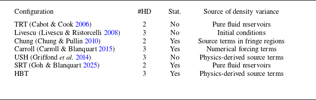
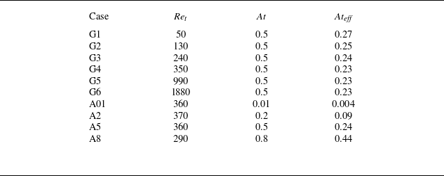
 Sc=1
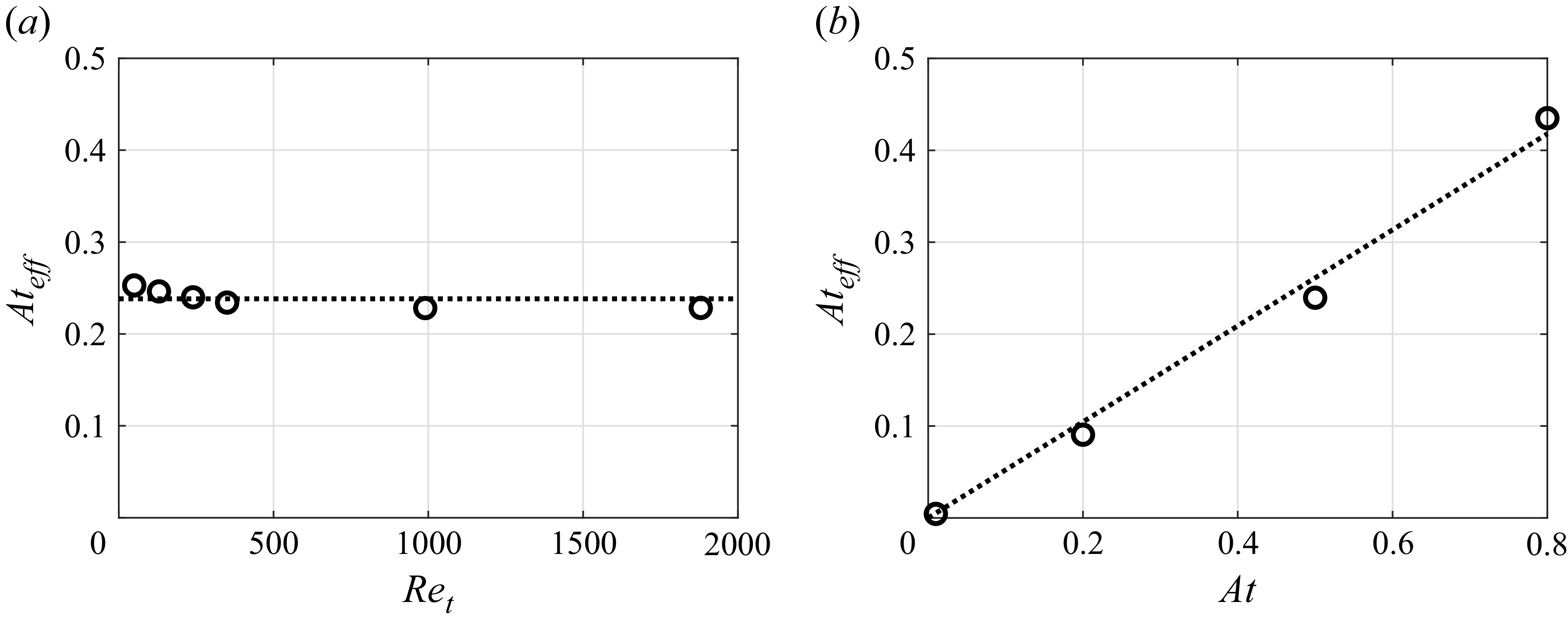
 Ateff=ρrms/ρ¯
 Ret
 At=(ρH−ρL)/(ρH+ρL)
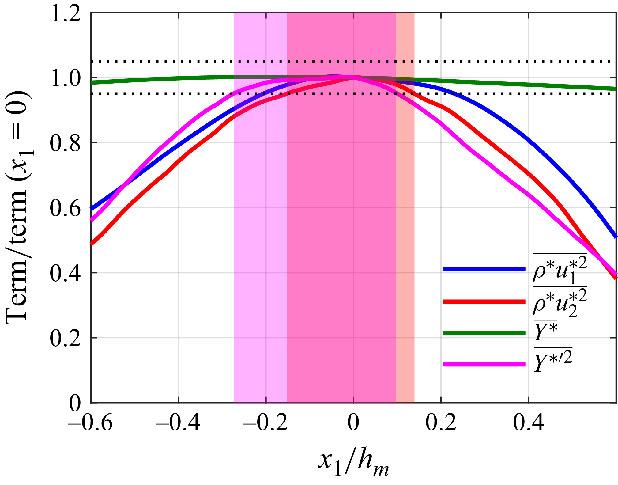
 ρ∗u2∗2¯
 Y∗′2¯
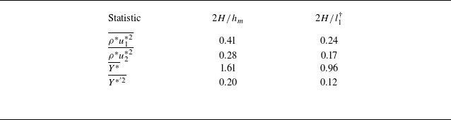
 H
 5%

 C1
 i

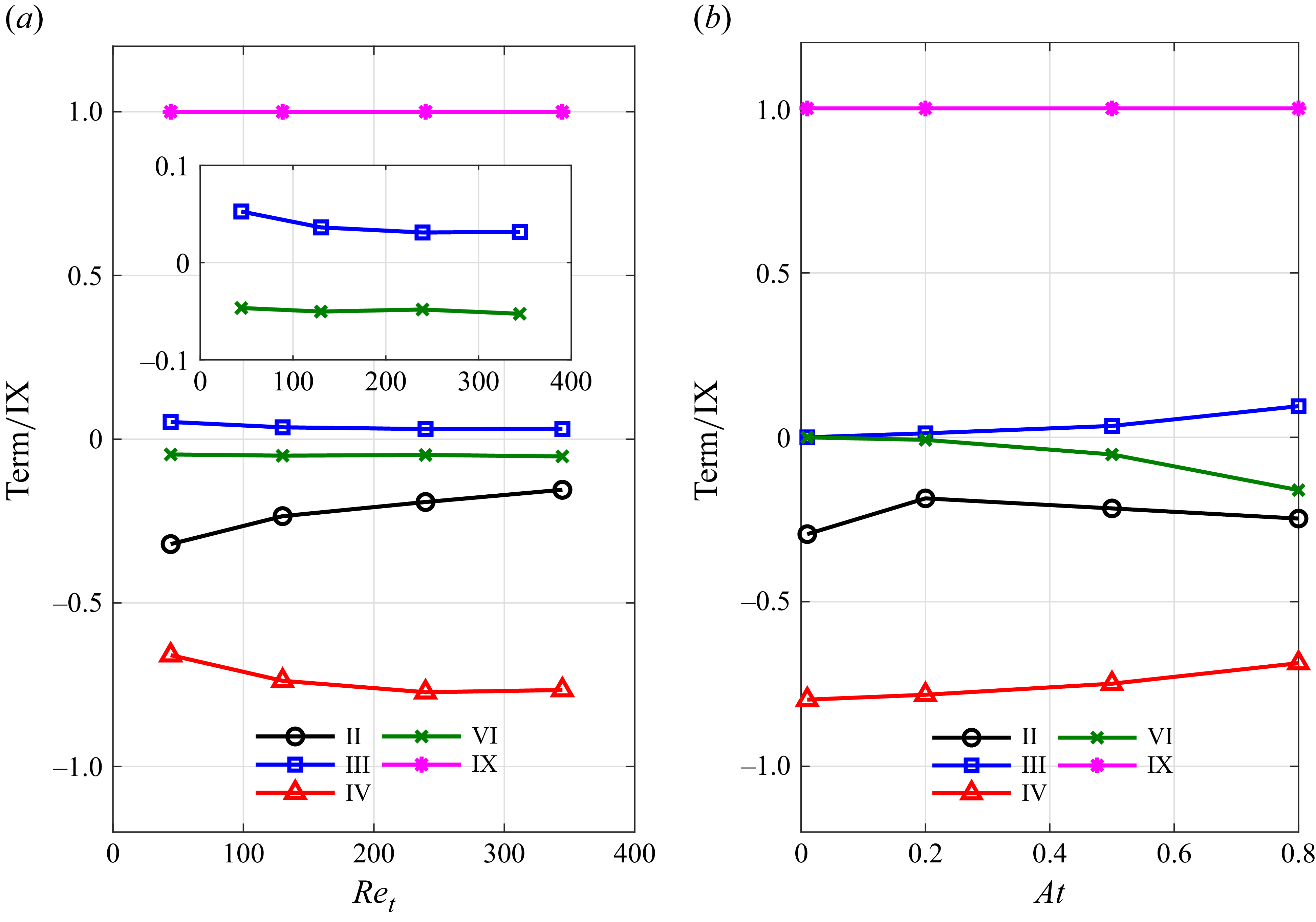
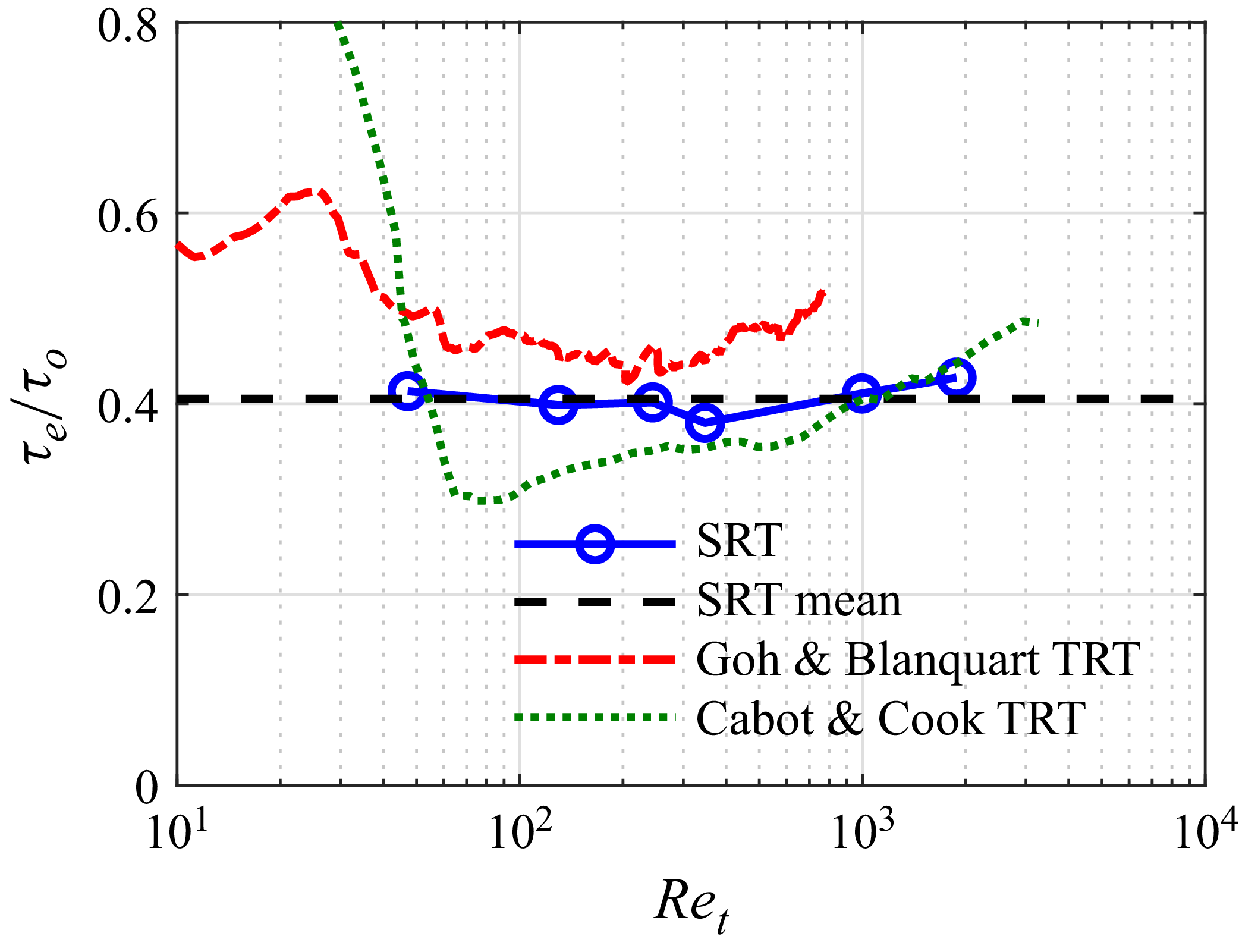
 τt/τo
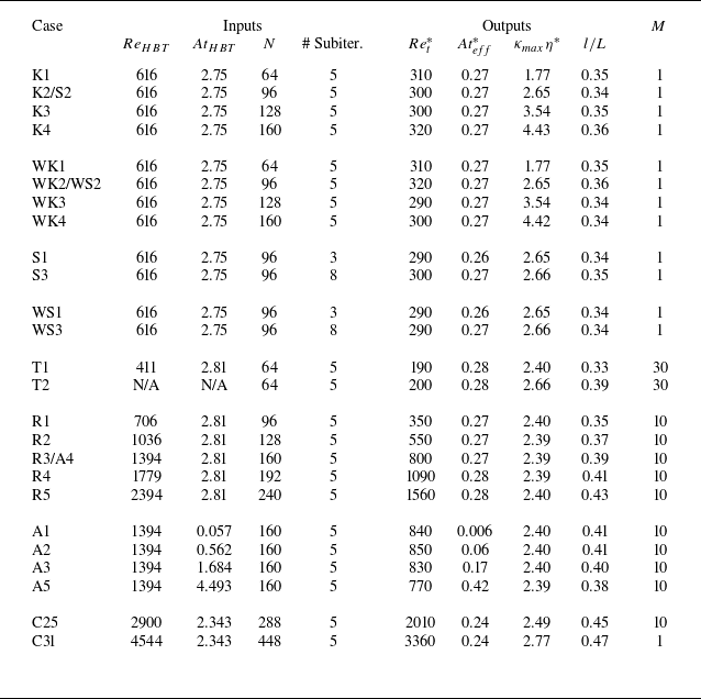

 At=0.5
 ≈6400
 ρL
 ρ¯
 l

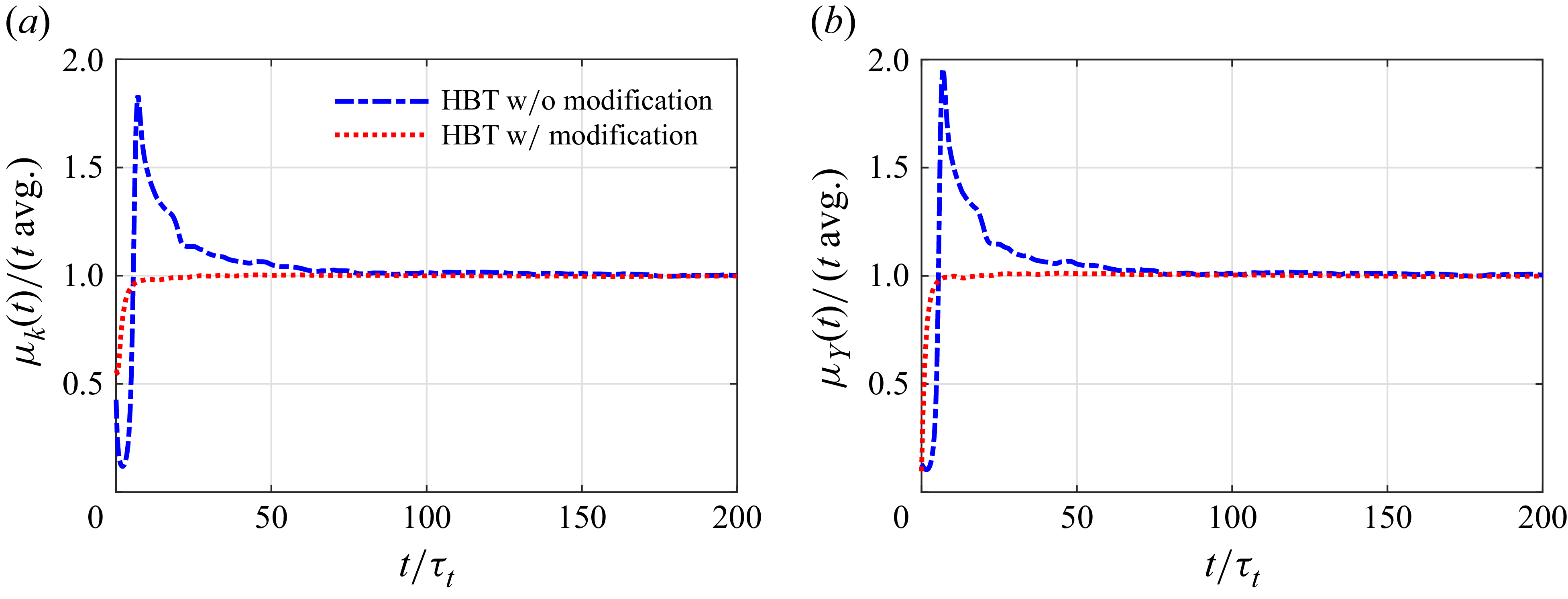

 τcorr


 CRe
 CAt
 ReHBT
 CRe
 CAt

 CRe
 CAt
 AtHBT
 CRe
 CAt


 κ


 t=25τΔ

 t=25τΔ
 x1
 i
 j

 t=31τΔ
 ϵ~
 ν
 x1
 i
 10−5

 t=31τΔ
 κη=3
 x1

 t=31τΔ
 ϵ~
 ϵρ
 ν
 x1
 10−5

 t=31τΔ
 ϵ~
 ϵρ
 ν
 x1
 10−5

 t=31τΔ
 Eρ12-D
 Eρρ2-D
 E112-D
 Eρ12-D
 Eρρ2-D
 E112-D
 x1

 40τt