1. Introduction
Turbulent gravity currents are produced when a finite volume of dense fluid is rapidly released from a source above a horizontal boundary into an environment of lower density. The dense fluid spreads horizontally under gravity along the lower boundary of the flow domain, displacing the original fluid in place. Gravity currents have been studied in considerable detail, using a combination of laboratory experiments and mathematical models, owing to their importance in frontal dynamics, volcanic eruptions, turbidity currents and many environmental flows (Prandtl Reference Prandtl1952; Sparks et al.
Reference Sparks, Bursik, Carey, Gilbert, Glaze, Sigurdsson and Woods1997; Simpson Reference Simpson1999; Kneller & Buckee Reference Kneller and Buckee2000). Many papers have examined two-dimensional gravity currents in a confined channel with parallel sides, exploring the ratio of the propagation speed of the front,
 $\text{d}r_{n}/\text{d}t$
, with the product of the buoyancy and depth,
 $g^{\prime }h$
, as expressed by the Froude number,
 $Fr$
,
 $\text{d}r_{n}/\text{d}t=Fr(g^{\prime }h)^{1/2}$
. Various solutions of shallow water equations have been presented to describe these flows, often assuming that there is no mixing with the ambient fluid (cf. Benjamin Reference Benjamin1968; Chen Reference Chen1980; Bonnecaze et al.
Reference Bonnecaze, Hallworth, Huppert and Lister1995; Slim & Huppert Reference Slim and Huppert2004).
Huppert & Simpson (Reference Huppert and Simpson1980) carried out experiments to examine the motion of axisymmetric gravity currents produced by a discrete release of fluid of total buoyancy
 $B$
, and established that, provided the Reynolds number is sufficiently high, the front of the current advances as
 $r_{n}=1.3B^{1/4}t^{1/2}$
. Hallworth et al. (Reference Hallworth, Phillips, Huppert and Sparks1993, Reference Hallworth, Huppert, Phillips and Sparks1996) and Hacker, Linden & Dalziel (Reference Hacker, Linden and Dalziel1996) measured the entrainment of ambient fluid into gravity currents, and established that the head becomes progressively more dilute with distance. Hallworth et al. (Reference Hallworth, Huppert, Phillips and Sparks1996) used an acid–alkali system with which the mixing in the head could be measured by assuming the head is well mixed and recording the position of the head at which a pH indicator in the head changed colour. Using this approach, they reported a gradual decrease in the volume of the head with distance. Patterson et al. (Reference Patterson, Simpson, Dalziel and van Heijst2006) carried out some PIV experiments to explore the velocity structure of the current, and this demonstrated that the front of an axisymmetric gravity current involves a vortical flow that facilitates the mixing between the current fluid recirculating over the top of the nose and the ambient fluid displaced by the nose. Cantero, Balachandar & Garcia (Reference Cantero, Balachandar and Garcia2007a
) and Cantero et al. (Reference Cantero, Lee, Balachandar and Garcia2007b
) presented a series of direct numerical simulations of axisymmetric gravity currents, illustrating the importance of the vortex rings and cleft and lobe instabilities at the front of the flow in driving mixing. Adduce, Sciortino & Proietti (Reference Adduce, Sciortino and Proietti2012) and Johnson & Hogg (Reference Johnson and Hogg2013) modelled the mixing into two-dimensional gravity currents using a parameterised entrainment law all along the upper surface of the flow, while Özgökmen, Iliescu & Fischer (Reference Özgökmen, Iliescu and Fischer2009) have presented numerical simulations of the mixing. More recent experiments by Sher & Woods (Reference Sher and Woods2015) quantified the mixing into the head of a two dimensional gravity current.
Although these have been very valuable contributions, there is more to be learnt about the process of mixing and entrainment into axisymmetric gravity currents through detailed measurement of the buoyancy as a function of position in the current and time after the lock release. This is the primary purpose of the present paper. We use a light attenuation technique to measure the evolving salinity of the fluid in aqueous saline gravity currents (cf. Hacker et al.
Reference Hacker, Linden and Dalziel1996). For the low salt concentrations used in our experiments, the salinity is directly proportional to the buoyancy (Turner Reference Turner1979) and the Boussinesq approximation applies. We also follow pulses of dye in the current and the ambient fluid to establish how the mixing occurs. Using our new experimental data, we find that a fraction
 $E\sim 0.33\pm 0.09$
of the fluid ahead of the current, which is displaced by the current, mixes with the recirculating current fluid. This mixed fluid is distributed between the wake and head of the flow, producing a vertically and radially stratified flow. We establish scalings for the speed, height, vertically averaged buoyancy and Froude number of the head, based on our experimental data. We then compare the experimental depth and buoyancy profiles in the flow with an idealised self-similar solution derived from the depth-averaged equations of motion, in which we account for the mixing at the head and the vertical shear and stratification in the flow.
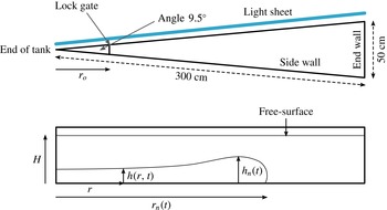
Schematic diagram of the experimental tank, showing a top view and a side view of the tank. The figure also illustrates the depth
 $h$
of the current at radius
 $r$
, the maximum depth
 $h_{n}$
, the position of the nose of the current
 $r_{n}$
, and the radius of the lock gate
 $r_{o}$
.

2. Experimental method
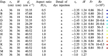
A series of turbulent laboratory gravity currents were generated through the release of a finite volume of aqueous salt solution into a 3 m long Perspex tank with free surface at the top. The width of the tank increases from 0 to 50 cm along the length of the tank until it reaches the end wall. The two long sidewalls subtend an angle of approximately
 ${\sim}9.5^{\circ }$
(figure 1). The details of the parameters for each experiment are shown in table 1, including the depth of the fluid,
 $H$
, the radius of the lock gate,
 $r_{o}$
, and the aspect ratio of the source,
 $H/r_{o}$
, as well as the initial buoyancy associated with the salinity,
 $g_{o}^{\prime }=g({\it\rho}_{s}-{\it\rho}_{w})/{\it\rho}_{w}$
where
 $g$
is the acceleration due to gravity,
 ${\it\rho}_{s}$
is the density of the saline water behind the lock gate and
 ${\it\rho}_{w}$
is the density of the fresh water (ambient fluid). The volume and buoyancy in our experiments overlap those used in many of the previous experimental studies of axisymmetric gravity currents (Huppert & Simpson Reference Huppert and Simpson1980; Hallworth et al.
Reference Hallworth, Huppert, Phillips and Sparks1996; Patterson et al.
Reference Patterson, Simpson, Dalziel and van Heijst2006) as well as the numerical study of Cantero et al. (Reference Cantero, Balachandar and Garcia2007a
). In many of the experiments, the aqueous solution was initially dyed with a known mass of red TRS food dye, and the tank was back-lit using a matrix LED light panel (W
 $\&$
Co Displays and Signs). In order to measure the dilution of the current associated with the mixing, solutions with different concentrations of dye were placed in the experimental tank, in sequence, and the red–green–blue (RGB) light intensity was recorded for each such solution at each point on one of the vertical walls of the tank using a Nikon D90 RGB DSLR camera.
Table of experiments illustrating range of aspect ratio and dimensions of the lock. a, light attenuation experiment; b, dye injected into head of the flow; c, dye injected into the ambient fluid. The column of colours indicates colours of data shown in subsequent graphs. The quantities
 $t_{o}$
,
 $\mathscr{R}$
and
 $Fr$
are properties of the current that are defined in § 3.3. In the table, for each experiment, we list the asymptotic values of
 $\mathscr{R}$
and
 $Fr$
for
 $r_{n}>3r_{o}$
(figure 5
a,b).

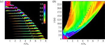
(a) Photographs of a saline gravity current illustrating the evolution of the buoyancy, shown by false-colour contours, as the current from experiment H (table 1) advances along the flume. Images are taken at equal time intervals of 1.5 s. The
 $x$
-axis shows the position in the current as a function of the number of lock lengths. The colour scale represents the value
 $g^{\prime }/g_{o}^{\prime }$
, which is the local buoyancy,
 $g^{\prime }$
, measured as a fraction of the original buoyancy,
 $g_{o}^{\prime }$
. (b) Evolution of the depth-averaged buoyancy of the flow as a function of position and time. The horizontal axis represents the horizontal position,
 $r/r_{o}$
, and the vertical axis is time. The colours represent the depth-averaged buoyancy of the gravity current, with the legend illustrating the fraction of original buoyancy of the fluid that was released from behind the lock gate. The triangles in the figure denote the horizontal position at which the volume of the current in the region between the back of the lock and the triangle equals 25 % of the total volume of the current (see figure 6
b).

The images were analysed using a MATLAB script to generate calibration curves relating light intensity to the salinity,
 $s$
, and hence buoyancy,
 $g^{\prime }=g\mathscr{S}s$
, where
 $\mathscr{S}$
is the solutal expansion coefficient, following an approach analogous to Hacker et al. (Reference Hacker, Linden and Dalziel1996), van Sommeren, Caulfield & Woods (Reference van Sommeren, Caulfield and Woods2012) and Fragoso, Patterson & Wettlaufer (Reference Fragoso, Patterson and Wettlaufer2013). Since the width of the channel varies with radius, we used different local calibration curves, dividing the tank wall into individual regions each spanning
 $1~\text{cm}\times 1~\text{cm}$
. The experimental images can then be analysed to determine the distribution of buoyancy within the tank, accounting for the effects of the varying width of the tank on the light attenuation by using the local calibration curves. The buoyancy data we obtain are a span-wise average. However, owing to the small angle subtended by the two sidewalls of the tank, the variation in the radius across a span, as measured from the rear of the lock gate, is less than 0.5 % of the radius. We therefore interpret our data as providing an approximation for the radial distribution of buoyancy. The camera was set to take either 2 or 4 frames per second with shutter speed
 $1/100$
, aperture
 $F4.8$
and ISO 640. The precise timing of the images was checked carefully in a control experiment. The camera recorded
 $10~\text{pixels}~\text{cm}^{-1}$
in the vertical and horizontal directions throughout the flow domain. Most of the currents attained high Reynolds number,
 $Re=(h_{n}/{\it\nu})(\text{d}r_{n}/\text{d}t)>5000$
where
 ${\it\nu},h_{n}$
and
 $r_{n}$
are the kinematic viscosity, maximum depth of the current and position of the nose respectively. We estimate that the image calibration method used to convert light intensity to buoyancy has an error less than 8 % for all experiments, and this is reflected in the error bars presented in our analysis.
3. Experimental observations
Figure 2(a) illustrates the time evolution of the gravity current for experiment H (table 1). The sequence of false-colour images correspond to the buoyancy of the fluid in the tank at intervals of 1.5 s after release of the lock gate. Immediately after lock release, while the position of the nose,
 $r_{n}$
, is close to the source,
 $r_{n}<2.5r_{o}$
, the current adjusts to a head–tail structure. Subsequently, as the front advances through the region
 $2.5r_{o}<r_{n}<8r_{o}$
, the current becomes progressively less dense and stratified in both the vertical and horizontal directions. The maximum density arises in the lower part of the head of the flow. With time, the head region develops a strong vortical structure, with the dense fluid lower in the head reaching the front of the head, and rising up over the head. Here it mixes with ambient fluid as it recirculates backwards relative to the head. In figure 2(b), we illustrate the evolution of the vertically averaged buoyancy of the current as a function of radius. In the figure, a series of triangles are shown, such that the volume of the current between the back of the lock and the triangle is a fraction 0.25 of the total volume of the current. The image illustrates that the vertically averaged buoyancy of the current in the region ahead of the triangles progressively decreases with time and increases in the radial direction, with the vertically averaged buoyancy being largest just behind the leading front of the current. In panel (a), it can be seen that the current is very thin in the region upstream of the triangles, and in this region the flow appears to become controlled by bottom friction. The fluid that lags behind in this bottom layer appears to be relatively dense fluid from the base of the flow, as may seen in panel (b), where the vertically averaged buoyancy increases upstream of the triangles.
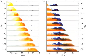
Series of images of the current at successive times. (a) Transport of a pulse of red dye injected just behind the front of the flow in the head (experiment M). This shows how the dyed fluid in the current advances to the front of the flow, and then recirculates over the top of the current. Here it mixes with the ambient fluid, which is displaced up over the advancing head of the flow. (b) Transport of dyed blue ambient fluid injected just ahead of the front of the red current (experiment N). Some of the ambient fluid displaced by the current remains above the current after the head has passed by, and hence does not mix with the current, while the remainder mixes into current, recirculating in the flow.

3.1. Mechanism of mixing
In order to build up understanding of how the mixing occurs, we have carried out a series of experiments in which we inject and then track a small volume of dye in both (i) the current and (ii) the ambient fluid. Figure 3(a) illustrates the progress of a yellow gravity current advancing into a clear ambient fluid (experiment M, table 1). In this experiment, a pulse of red dye was injected at
 $r=3r_{o}$
into the current, when the nose of the current reached the position
 $r_{n}=3.5r_{o}$
. The dye pulse is observed to migrate forwards relative to the front of the current, and on reaching the front of the current, the dyed fluid rises to the top of the current and recirculates backwards relative to the front. Here it seems to mix with some of the ambient fluid originally ahead of the current, which is displaced up and over the current. Similar mixing behaviour was observed in numerous other experiments in which dye was injected behind the front of the current but with the front of the current located at different radial distances from the lock.
We also added dye to the ambient fluid to provide a complementary perspective on the mixing in the head region of the flow. As seen in figure 3(b), the red gravity current in experiment N (table 1) displaced a region
 $5.2r_{o}<r<5.5r_{o}$
in which the ambient fluid originally ahead of the current was dyed blue. The images show that the ambient fluid dyed blue rises over the current and there is some mixing with the recirculating current fluid. The mixed fluid migrates backwards relative to the advancing head and becomes partitioned into the head and tail of the current. Meanwhile, the remainder of the displaced ambient fluid (blue) rises up over the head, and comes to rest once the head has passed by.
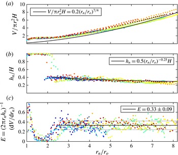
Variation as a function of
 $r_{n}/r_{o}$
of (a) the volume of the current, (b) the height of the head of the current in the region
 $r_{o}<r_{n}<8r_{o}$
and (c) the entrainment coefficient
 $E$
defined by (3.2) and estimated from the experimental data shown in (a) and (b).

3.2. Entrainment coefficient
Using the light attenuation technique, we have measured the instantaneous volume of the whole current and the maximum depth of the head as a function of the radius of the front of the current by determining those pixels for which the concentration of dye is in excess of the original value (figure 4
a,b). Once we have measured the volume,
 $V_{e}$
, in our experimental sector model, of angle
 ${\it\phi}$
, we convert this to an equivalent volume
 $V$
of a fully axisymmetric current,
 $V=(2{\rm\pi}/{\it\phi})V_{e}$
. We also define the total buoyancy
 $B$
as that of the equivalent fully axisymmetric current,
 $B=(2{\rm\pi}/{\it\phi})B_{e}$
where
 $B_{e}=g_{o}^{\prime }V_{e}$
is the actual total buoyancy of the fluid behind the lock gate. In the figure, the volume,
 $V(t)$
, and maximum depth,
 $h_{n}(t)$
, are presented in dimensionless form,
 $V/({\rm\pi}r_{o}^{2}H)$
and
 $h_{n}/H$
. Although there is some fluctuation in the volume and depth measurement associated with the time-dependent billow structures on the upper surface of the flow (figure 2), to reasonable approximation, for
 $r_{n}>2.5r_{o}$
, the data follow the approximate relations
 $$\begin{eqnarray}V=(0.2\pm 0.02){\rm\pi}r_{n}^{7/4}r_{o}^{1/4}H\quad \text{and}\quad h_{n}=(0.5\pm 0.02)H(r_{o}/r_{n})^{1/4}.\end{eqnarray}$$
If we assume that the fluid entrained into the current originates from the fluid displaced by the head of the flow, as indicated by the dye studies, and we define
 $E$
to be the fraction of this fluid that is entrained into the flow, we can write
 $$\begin{eqnarray}\frac{\text{d}V}{\text{d}t}=2{\rm\pi}Er_{n}h_{n}\frac{\text{d}r_{n}}{\text{d}t}.\end{eqnarray}$$
Noting
 $\text{d}V/\text{d}t=(\text{d}V/\text{d}r_{n})(\text{d}r_{n}/\text{d}t)$
, and using the data shown in figure 4(a,b), we find that for
 $2.5r_{o}<r_{n}<7r_{o}$
, the entrainment coefficient
 $E=0.33\pm 0.09$
(figure 4
c). The approximate scaling laws (3.1), which combined with (3.2) suggest
 $E=0.35\pm 0.04$
, are consistent with this direct measurement from the data. We note that in the region
 $r_{o}<r_{n}<1.4r_{o}$
the entrainment coefficient decreases rapidly from about 0.7 to 0.05. This is associated with the mixing across the near-vertical interface produced from the removal of the lock gate. The mixing then remains small as the flow slumps from the lock and the head becomes established. Then, as the head moves through the region
 $2r_{o}<r_{n}<2.5r_{o}$
,
 $E$
increases to the value
 $E=0.33\pm 0.09$
, which applies for
 $r_{n}>2.5r_{o}$
.
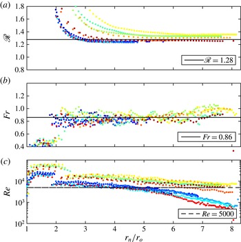
Data from experiments A–L (table 1) illustrating (a) the variation with time of
 $\mathscr{R}=r_{n}(t)/B^{1/4}(t+t_{o})^{1/2}$
, where
 $r_{n}$
is the position of the nose of the current as a function of time; (b) the variation with time of the Froude number,
 $Fr=\text{d}r_{n}/\text{d}t\,(\overline{g_{n}^{\prime }}h_{n})^{-1/2}$
, where
 $(\overline{g^{\prime }}h)_{n}$
is the maximum value of the vertical integral of buoyancy as a function of the position in the current; (c) the variation of the Reynolds number in the head with time. The data that fall below
 $Re=5000$
appear to be influenced by friction, and are not shown in panels (a,b).

3.3. Scaling laws for the head
We also measured the position of the nose,
 $r_{n}(t)$
, and the maximum value of the vertical integral of the buoyancy as a function of time. In figure 5(a), we illustrate the variation of the ratio
 $$\begin{eqnarray}\mathscr{R}=\frac{r_{n}(t)}{B^{1/4}(t+t_{o})^{1/2}},\end{eqnarray}$$
with
 $r_{n}/r_{o}$
, and find that, after an initial transient,
 $\mathscr{R}\rightarrow 1.28\pm 0.05$
consistent with the value
 $1.3$
reported by Huppert & Simpson (Reference Huppert and Simpson1980). In calculating
 $\mathscr{R}$
, for each experiment, we have estimated a value of the virtual origin in time,
 $t_{o}$
, by plotting
 $r_{n}^{2}$
as a function of time,
 $t$
, and finding the time
 $-t_{o}$
at which the best-fit straight line through the data intersects the time axis. This corresponds to the difference between the initial adjustment phase after removing the lock gate, when
 $r_{n}<2.5r_{o}$
, and the idealised release of a point source of buoyancy of zero volume. We find that
 $t_{o}$
decreases in magnitude from
 $-3.5$
to
 $-1.5~\text{s}$
, as the aspect ratio of the source,
 $H/r_{o}$
, decreases from 1.0 to 0.4. These values are considerably shorter than the 25–
 $30~\text{s}$
typically required for the current to travel to a distance
 $r_{n}\approx 7{-}8r_{o}$
.
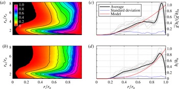
Variation with position
 $r/r_{n}$
of (a) the buoyancy in the current between the source and radius
 $r$
as a fraction of the total buoyancy,
 $\int _{0}^{r}r\overline{g^{\prime }}h\,\text{d}r/\int _{0}^{r_{n}}r\overline{g^{\prime }}h\,\text{d}r$
(experiment H), (b) the volume of the current in the region between the source and the position
 $r$
as a fraction of the total volume,
 $\int _{0}^{r}rh\,\text{d}r/\int _{0}^{r_{n}}rh\,\text{d}r$
(experiment H), (c) profiles of the dimensionless vertical integral of buoyancy (3.5a
) and (d) profiles of the dimensionless depth (3.5b
). (a,b) The black contour lines denote the horizontal location where the fraction of (a) the total buoyancy or (b) the total volume exceeds the value 0.1,
 $0.2,\ldots ,1.0$
. (c,d) Grey profiles denote the time average for each of the experiments A–L. The ensemble averages, standard deviations from these ensemble averages and the prediction of the simplified similarity solution (3.12) are shown in black, blue and red profiles respectively.

Earlier studies have proposed that the Froude number at the head of the current is a constant. Using our light attenuation data, we have measured the maximum value of the vertical integral of buoyancy in the current. This maximum occurs near the front of the current (figure 6
b), and by combining this with the speed of the nose we can calculate the Froude number,
 $Fr$
, as given by
 $$\begin{eqnarray}\frac{\text{d}r_{n}}{\text{d}t}=Fr\sqrt{(\overline{g^{\prime }}h)_{n}}\quad \text{where }(\overline{g^{\prime }}h)_{n}=\max \left(\overline{g^{\prime }}h=\int _{0}^{h(r)}g^{\prime }\,\text{d}y\right).\end{eqnarray}$$
Here
 $g^{\prime }(r,y,t)$
is the buoyancy in the current and (3.4b
) defines the vertically averaged buoyancy,
 $\overline{g^{\prime }}$
. The variation of
 $Fr$
as a function of the dimensionless time for our experimental currents A–L (table 1) is shown in figure 5(b). It is seen that for
 $r_{n}>2.5r_{o}$
,
 $Fr\rightarrow 0.86\pm 0.07$
, once the current has passed through an initial adjustment region. Combining (3.3) and (3.4), we find
 $(\overline{g^{\prime }}h)_{n}\approx (0.89\pm 0.12)B/r_{n}^{2}$
.
For each of the experiments shown in figure 5, the Reynolds number at the head of the flow remained in excess of 5000 (figure 5
c). In other experiments, for which the initial volume of fluid was smaller, we found that once the Reynolds number at the head falls below a value of about 5000, the value of
 $\mathscr{R}$
(3.3) gradually decreased with distance along the tank. We focus on flows with higher Reynolds number, although given the size of our experimental system this limits the study to currents for which
 $r_{n}<8r_{o}$
. Over this range our experimental data appear to follow the scaling laws as proposed in (3.1)–(3.3) but it would be of interest to carry out experiments in a larger facility with much larger currents.
3.4. Structure of the current
In the contour plot, figure 6(a), we show how the buoyancy in the current between the source and radius
 $r$
, as a fraction of the total buoyancy,
 $\int _{0}^{r}r\overline{g^{\prime }}h\,\text{d}r/\int _{0}^{r_{n}}r\overline{g^{\prime }}h\,\text{d}r$
, varies with the position in the current,
 $r/r_{n}$
(horizontal axis), and also with time, as represented by the position of the nose,
 $r_{n}/r_{o}$
(vertical axis). Similarly, in panel (b) we show how the fractional volume of the current in the region between the source and the position
 $r$
,
 $\int _{0}^{r}rh\,\text{d}r/\int _{0}^{r_{n}}rh\,\text{d}r$
, varies with position
 $r/r_{n}$
and time, as represented by
 $r_{n}/r_{o}$
. The black contour lines denote the position in the current,
 $r/r_{n}$
, at which the fraction of the total buoyancy (a) or of the total volume (b) exceeds the values 0.1,
 $0.2,\ldots ,1.0$
as a function of time, as represented by
 $r_{n}/r_{o}$
. Figures 6(a) and 6(b) were calculated for experiment H but are typical of all experiments A–L (table 1).
Profiles of the dimensionless vertical integral of the buoyancy and of the dimensionless depth, as given by
 $$\begin{eqnarray}\overline{g^{\prime }}h(r,t)/(\overline{g^{\prime }}h)_{n}(t)\quad \text{and}\quad h(r,t)/h_{n}(t),\end{eqnarray}$$
have been averaged over the time during which
 $2.5r_{o}<r_{n}<7r_{o}$
, for each of the experiments A–L. The time-average profiles are shown as light grey lines in figure 6(b,d). The ensemble average of these profiles is shown as the solid black line, and the standard deviation associated with the difference between the individual profiles and this ensemble average is indicated by the blue line.
The strong vortical motion in the leading part of the current can be seen to have an important influence on the profiles; there is in fact a local minimum in the depth-integrated buoyancy in the region
 $0.7<r/r_{n}<0.9$
.
Figure 6(b) shows that, for
 $r_{n}>2.5r_{o}$
, the contours of constant fractional volume have an approximately constant position in the current as the current advances and grows (figure 4
a). However, figure 6(a) shows that there is some variation with time of the position within the current at which different fractions of the total buoyancy of the current occur. In particular, as the current advances forward, a progressively larger fraction of the buoyancy appears to be left in the wake of the flow. The line of triangles in figure 2, located at
 $r/r_{n}\approx 0.7$
, seems to delineate a transition from a deeper active part of the flow,
 $r/r_{n}\geqslant 0.7$
, to a shallow wake,
 $r/r_{n}<0.7$
. Figures 6(a) and 6(b) also illustrate that, while
 $2.5r_{o}<r_{n}<7r_{o}$
, this active leading part of the current,
 $0.7<r/r_{n}<1.0$
, accounts for about
 $75\,\%$
of the current volume and in excess of
 $75\,\%$
of the buoyancy of the current. Owing to the slow loss of buoyancy from the front of the current into the wake (figure 6
a), the current is not strictly self-similar. However, given the scalings in the head of the current (figures 4, 5), and given that the contours of fractional volume of the current are approximately independent of time for
 $2.5r_{o}<r_{n}<7r_{o}$
(figure 6
b), it is of interest to compare the data with some new self-similar solutions of the depth-averaged equations that account for the entrainment in the head (3.2).
3.5. A depth-averaged model
The equations for conservation of mass, momentum and buoyancy have the form (cf. Chen Reference Chen1980; Bonnecaze et al. Reference Bonnecaze, Hallworth, Huppert and Lister1995)
 $$\begin{eqnarray}\displaystyle & \displaystyle \frac{\partial (rh)}{\partial t}+\frac{\partial (rh\bar{u})}{\partial r}=0, & \displaystyle\end{eqnarray}$$
 $$\begin{eqnarray}\displaystyle & \displaystyle \frac{\partial (rh\bar{u})}{\partial t}+\frac{\partial ({\it\beta}rh\bar{u}^{2})}{\partial r}=-\frac{\partial ({\it\gamma}rh^{2}\overline{g^{\prime }})}{\partial r}-\frac{rh}{{\it\rho}}\frac{\partial p}{\partial r}, & \displaystyle\end{eqnarray}$$
 $$\begin{eqnarray}\displaystyle & \displaystyle \frac{\partial (rh\overline{g^{\prime }})}{\partial t}+\frac{\partial ({\it\alpha}rh\overline{g^{\prime }}\bar{u})}{\partial r}=0, & \displaystyle\end{eqnarray}$$
 ${\it\rho}$
is a representative density,
 $p$
the pressure, and the depth-averaged properties are defined as
 $$\begin{eqnarray}\left.\begin{array}{@{}c@{}}\displaystyle h\bar{u}=\int _{0}^{h}u\,\text{d}y;\quad {\it\beta}h\bar{u}^{2}=\int _{o}^{h}u^{2}\,\text{d}y;\quad h\overline{g^{\prime }}=\int _{0}^{h}g^{\prime }\,\text{d}y;\\ \displaystyle {\it\alpha}h\overline{g^{\prime }}\bar{u}=\int _{0}^{h}ug^{\prime }\,\text{d}y\quad \text{and}\quad {\it\gamma}h^{2}\overline{g^{\prime }}(r,t)=\int _{0}^{h}\int _{y}^{h}g^{\prime }(r,y,t)\,\text{d}y\,\text{d}y^{\prime }.\end{array}\right\}\end{eqnarray}$$
In contrast to earlier models (Chen Reference Chen1980; Bonnecaze et al.
Reference Bonnecaze, Hallworth, Huppert and Lister1995), we have included the coefficients
 ${\it\alpha}$
,
 ${\it\beta}$
and
 ${\it\gamma}$
(3.9) that arise from the vertical gradient of the horizontal velocity and the buoyancy in the flow, as illustrated in figures 2 and 3 (cf. Kneller & Buckee Reference Kneller and Buckee2000).
 ${\it\alpha}$
and
 ${\it\beta}$
represent the advection speed of the reduced gravity and momentum relative to that of the vertically averaged flow. In principle these coefficients may vary along the direction of flow, for example in the nose region.
As a result of the entrainment (3.2), we can integrate (3.6) to show that the vertically averaged mean fluid speed at the front,
 $\bar{u}(r_{n})$
, is given by
 $$\begin{eqnarray}\bar{u}(r_{n})=(1-E)\frac{\text{d}r_{n}}{\text{d}t}.\end{eqnarray}$$
This relation is consistent with the entrainment that occurs in the nose since there is a vertical shear in the flow (figure 3). The conservation of buoyancy requires that
 $$\begin{eqnarray}2{\rm\pi}\int _{0}^{r_{n}}rh(r,t)\overline{g^{\prime }}(r,t)\,\text{d}r=B.\end{eqnarray}$$
Guided by the scalings given in (3.1)–(3.3), it may be shown that, in the simplified situation in which
 ${\it\alpha},{\it\beta}$
and
 ${\it\gamma}$
are assumed to be constant and independent of position, these equations have self-similar solutions of the form
 $$\begin{eqnarray}h(r,t)=\mathscr{H}H\left(\frac{r_{o}}{r_{n}}\right)^{1/4}{\it\eta}^{{\it\omega}};\quad \overline{g^{\prime }}(r,t)=\mathscr{G}\frac{B^{1/2}}{tH}\left(\frac{r_{o}}{r_{n}}\right)^{-1/4}{\it\eta}^{2-{\it\omega}};\quad \bar{u}(r,t)=\mathscr{U}B^{1/4}t^{-1/2}{\it\eta},\end{eqnarray}$$
where
 ${\it\eta}=r/r_{n}(t)$
,
 $r_{n}(t)=\mathscr{R}B^{1/4}t^{1/2}$
and
 ${\it\omega}$
,
 $\mathscr{G},\mathscr{H}$
and
 $\mathscr{U}$
are constants. Equations (3.6), (3.8), (3.10) and (3.11) then require that
 $$\begin{eqnarray}\mathscr{GH}=\frac{2}{{\rm\pi}\mathscr{R}^{2}};\!\quad \mathscr{U}=(1-E)\mathscr{R}/2;\!\quad {\it\alpha}=\frac{1}{1-E};\!\quad {\it\omega}=\frac{8E-7}{-4E}\quad \text{and}\quad Fr=\frac{\mathscr{R}}{(4\mathscr{G}\mathscr{H})^{1/2}}.\vphantom{\mathop{\sum }_{\sum }}\end{eqnarray}$$
Note that this solution is consistent with (3.7) and can be used to determine the pressure.
Given that we have found
 $\mathscr{R}=1.28\pm 0.05$
and
 $E=0.33\pm 0.09$
(figures 4
c, 5
a), the solution (3.12)–(3.13) suggests that
 $\mathscr{U}=0.42\pm 0.1$
,
 ${\it\alpha}=(1-E)^{-1}=1.5\pm 0.2$
,
 $Fr=1.0\pm 0.1$
and
 ${\it\omega}=3.3\pm 1$
. This estimate for the Froude number,
 $Fr=1.0\pm 0.1$
overlaps with the independent measurement of
 $Fr$
shown in figure 5(b),
 $0.86\pm 0.07$
, although it is a little higher.
These simplified similarity solutions that conserve the total buoyancy do therefore capture the speed and the buoyancy of the front, as well as the gradual increase in the total volume through entrainment. In figure 6(c,d), we compare the dimensionless solutions (3.12)
 $h(r,t)/h(r_{n},t)={\it\eta}^{{\it\omega}}$
and
 $\overline{g^{\prime }}(r,t)h(r,t)/\overline{g^{\prime }}(r_{n},t)h(r_{n},t)={\it\eta}^{2}$
with the experimental measurements of the depth and vertically averaged buoyancy along the current (3.5). As expected, the simplified solutions do not capture the full structure of the head, which is strongly influenced by the recirculation, but they do predict an increase in depth and buoyancy towards the front of the flow. It may be that by accounting for some variation in the shape factors
 ${\it\alpha},{\it\beta},{\it\gamma}$
in the head of the current, more of the structure may be determined, although this is beyond the scope of our measurements. Also, as
 $r_{n}$
increases, figure 6(a) suggests that the flow evolves from such a self-similar constant buoyancy solution owing to the gradual loss of buoyancy from the head into the wake (cf. figure 6
a).
4. Discussion
We have presented a new suite of experiments in which we measure the nose speed and the depth and evolving buoyancy throughout an axisymmetric gravity current produced by the release of a finite mass of dense fluid from behind a lock gate. We find that as the current advances it entrains a fraction
 $0.33\pm 0.09$
of the ambient fluid, which is displaced over the head of the flow. The current includes a region of recirculation near the head, which drives this mixing. To good approximation, the position and depth of the head follow the scaling laws
 $r_{n}\sim (1.28\pm 0.05)B^{1/4}t^{1/2}$
and
 $h_{n}\sim 0.5H(r_{o}/r_{n})^{1/4}$
, and the effective Froude number of the head of the flow is about
 $0.86\pm 0.07$
.
A depth-averaged model for the flow that accounts for the entrainment at the front, and the vertical shear in the velocity and buoyancy, leads to some new self-similar solutions that predict the increase in volume of the current with time, and also the increase in depth and salt content towards the front of the flow. However, the simplified model does not capture all the detailed structure of the recirculating flow in the head.
Our experiments have focused on flow spreading in a sector of a circle with angle
 $9.5^{\circ }$
in order that we can measure the buoyancy using the light attenuation technique (figure 1). Numerical simulations by Cantero et al. (Reference Cantero, Balachandar and Garcia2007a
) for a fully axisymmetric current illustrate the importance of the vortex ring structures that stretch and break up in the azimuthal direction. It would be interesting to develop an experimental technique to measure the mixing in such fully axisymmetric gravity currents for comparison with the present work.
The mixing process we have described has numerous implications for large-scale density-driven flows in nature and the environment whose Reynolds numbers are sufficiently high (
 $Re>5000$
). For example, in a current produced by a sudden release of dense gas, we predict that the concentration in the head will rapidly fall to 0.2–0.3 of the initial value as the flow spreads to distances of 6–7 times the original size of the gas release (figure 2
b). This modelling can therefore inform hazard assessment associated with dangerous concentrations of the gas. The work also has important implications for more complex geophysical and geological flows, and this will form a topic of further research.