1. Introduction
The collapse of a column of granular material has long served as a canonical test case for gaining insight into the mechanisms that govern granular flows, for identifying the different regimes and scaling laws to which they give rise (Lajeunesse, Mangeney-Castelnau & Vilotte Reference Lajeunesse, Mangeney-Castelnau and Vilotte2004; Lube et al. Reference Lube, Huppert, Sparks and Hallworth2004, Reference Lube, Huppert, Sparks and Freundt2005, Reference Lube, Huppert, Sparks and Freundt2007; Balmforth & Kerswell Reference Balmforth and Kerswell2005; Lajeunesse, Monnier & Homsy Reference Lajeunesse, Monnier and Homsy2005; Siavoshi & Kudrolli Reference Siavoshi and Kudrolli2005; Staron & Hinch Reference Staron and Hinch2005). Both dry and submerged collapses have been considered in the past, in two-dimensional as well as axisymmetric configurations, and on plane and sloping surfaces.
While the large majority of investigations to date have addressed cohesionless granular collapses, only a few studies have considered the effect of cohesive forces but under dry conditions (Rognon et al. Reference Rognon, Roux, Wolf, Naaïm and Chevoir2006; Mériaux & Triantafillou Reference Mériaux and Triantafillou2008; Berger et al. Reference Berger, Azéma, Douce and Radjai2016; Mandal, Nicolas & Pouliquen Reference Mandal, Nicolas and Pouliquen2020). These authors find a significant influence of the attractive interparticle forces on dry granular collapses, which suggests that they may also have the potential to alter submerged collapses. Artoni et al. (Reference Artoni, Santomaso, Gabrieli, Tono and Cola2013), Gabrieli et al. (Reference Gabrieli, Artoni, Santomaso and Cola2013), Santomaso, Volpato & Gabrieli (Reference Santomaso, Volpato and Gabrieli2018) and Zhou et al. (Reference Zhou, Ioannidou, Masoero, Mirzadeh, Pellenq and Bazant2019) have performed simulations and experiments that model cohesive forces via capillary bridges, and they observe the emergence of particle clusters. Langlois, Quiquerez & Allemand (Reference Langlois, Quiquerez and Allemand2015) studied particles initially held together by tensile bonds, which can be broken irreversibly during the collapse. Bougouin, Lacaze & Bonometti (Reference Bougouin, Lacaze and Bonometti2019) provided a diagram of the different regimes of cohesive collapse. Abramian, Staron & Lagrée (Reference Abramian, Staron and Lagrée2020) estimated the macroscopic yield stress based on the cohesive contacts between grains. Abramian, Lagrée & Staron (Reference Abramian, Lagrée and Staron2021) used the roughness of a cohesive granular deposit surface to investigate the formation of the clusters. Compared to a non-cohesive column, they find that the final deposit is much rougher as it contains large aggregates, and that the internal stratigraphic structure of the column is not preserved.
The influence of cohesion on submerged granular collapses, on the other hand, remains poorly understood at present, in spite of their importance for numerous industrial and environmental applications, e.g. immersed cohesive sediment flows (Kuenen Reference Kuenen1951; Hampton Reference Hampton1972; Marr et al. Reference Marr, Harff, Shanmugam and Parker2001; Baas, Best & Peakall Reference Baas, Best and Peakall2011). To address this issue, the current investigation will employ particle-resolving simulations in order to explore how the presence of cohesive forces modifies the dynamics of cohesionless submerged collapses. Such non-cohesive granular collapses have been studied extensively both via experiments (Rondon, Pouliquen & Aussillous Reference Rondon, Pouliquen and Aussillous2011; Bougouin & Lacaze Reference Bougouin and Lacaze2018; Lee, Huang & Yu Reference Lee, Huang and Yu2018; Yang et al. Reference Yang, Jing, Kwok and Sobral2021) and by means of numerical simulations (Topin et al. Reference Topin, Monerie, Perales and Radjai2012; Jing et al. Reference Jing, Yang, Kwok and Sobral2018, Reference Jing, Yang, Kwok and Sobral2019; Xu, Dong & Ding Reference Xu, Dong and Ding2019; Yang et al. Reference Yang, Jing, Kwok and Sobral2019, Reference Yang, Jing, Kwok and Sobral2020; Lacaze et al. Reference Lacaze, Bouteloup, Fry and Izard2021; Rauter Reference Rauter2021). These studies indicate that the dynamics of non-cohesive collapses, as well as their final height, runout distance and deposit morphology is governed primarily by the aspect ratio  $a=H_i/L_i$ of the column, where
 $H_i$ and
 $L_i$ denote its vertical and horizontal extents. In addition, the initial particle volume fraction
 $\phi$, the properties of the individual particles (diameter
 $d_p$, density
 $\rho _p$), and the ambient fluid (kinematic viscosity
 $\nu _f$, density
 $\rho _f$) have a noticeable influence on the collapse process as well. For cohesionless materials, two distinct modes of the initial collapse have been observed. For
 $a>3$ (Lee et al. Reference Lee, Huang and Yu2018), the failure surface, i.e. the interface between the static and moving particles, is buried deeply in the column, and initially the upper portion of the column descends approximately vertically. For
 $a<3$, on the other hand, initially the upper part of the column slides forward along a shallow failure surface. The final height and runout distance have been shown to follow power-law relationships with
 $a$ (Bougouin & Lacaze Reference Bougouin and Lacaze2018; Jing et al. Reference Jing, Yang, Kwok and Sobral2018; Lee et al. Reference Lee, Huang and Yu2018). Two additional critical aspect ratios govern the final shape of the deposit profile (Lee et al. Reference Lee, Huang and Yu2018). For
 $a< a_H$, where
 $a_H$ depends on the particle and fluid parameters, the final deposit profile has a trapezoidal shape; for
 $a>8$, it is shaped like a ‘Mexican hat’, with a steep central cone and an almost flat outer region, and otherwise it has a triangular shape.
The role of the initial volume fraction  $\phi$ can be understood via the pore pressure feedback mechanism proposed by Iverson et al. (Reference Iverson, Reid, Iverson, Lahusen, Logan, Mann and Brien2000). In submerged granular collapses, dense packings (high
 $\phi$ and negative pore pressure) result in slow dynamics and short runout distances, while loose packings (low
 $\phi$ and positive pore pressure) are associated with more rapid dynamics and longer runout distances (Rondon et al. Reference Rondon, Pouliquen and Aussillous2011; Topin et al. Reference Topin, Dubois, Monerie, Perales and Wachs2011; Yang et al. Reference Yang, Jing, Kwok and Sobral2020). The transition between these two regimes occurs near a critical value
 $\phi =0.58$ (Rondon et al. Reference Rondon, Pouliquen and Aussillous2011; Yang et al. Reference Yang, Jing, Kwok and Sobral2020). Rondon et al. (Reference Rondon, Pouliquen and Aussillous2011) and Bougouin & Lacaze (Reference Bougouin and Lacaze2018) also observe the existence of an initial relaxation time in a densely packed column before it starts to flow. Furthermore, hydroplaning can take place for sufficiently large loosely packed columns due to the fast-moving surge front, which reduces the frictional resistance dramatically and thereby results in a longer runout distance than their dry counterparts (Yang et al. Reference Yang, Jing, Kwok and Sobral2020).
Submerged granular collapses can be classified into three different categories (free-fall, inertial and viscous), depending on the particle and fluid properties (Bougouin & Lacaze Reference Bougouin and Lacaze2018; Jing et al. Reference Jing, Yang, Kwok and Sobral2019). The relevant regime is determined by two dimensionless numbers, the Stokes number  $St$ and the density ratio
 $r$:
 $$\begin{gather} St=\frac{1}{18\sqrt{2}}\,\frac{\sqrt{\rho_p(\rho_p-\rho_f)gd^{3}_p}}{\nu_f\rho_f}, \end{gather}$$
 $$\begin{gather}r=\sqrt{\frac{\rho_p}{\rho_f}}. \end{gather}$$
Courrech du Pont et al. (Reference Courrech du Pont, Gondret, Perrin and Rabaud2003) show that for  $St\gg 10$ and
 $r\gg 4$ the collapse is in the free-fall regime, for
 $St\gg 2.5r$ and
 $r\ll 4$ it is in the inertial regime, and otherwise it is in the viscous regime.
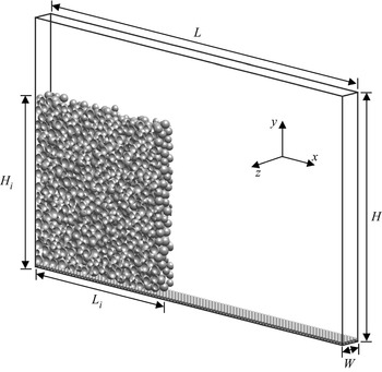
For submerged cohesive cases, our current knowledge is limited with regard to the formation and persistence of aggregates, and the internal structure of the final deposit. Furthermore, we do not have scaling laws for the dependence of the front velocity, the runout length and the deposit thickness on the cohesive force strength. The present study aims to provide such information for different aspect ratios. The particle-resolving simulations to be discussed below focus on the collapse of submerged granular columns within a tank of length  $L$, height
 $H$, and width
 $W$, as sketched in figure 1. Initially, the lower left section of the tank contains a granular column of length
 $L_i$ and height
 $H_i$, composed of spherical particles that are denser than the fluid. Section 2 presents the computational approach along with validation results. Section 3 focuses on the results of the simulations, in terms of the spreading velocity and runout distance, as well as the final height and structure of the deposit. The energy budget will be analysed in detail. Subsequently, the discussion will focus on particle-scale features of the collapse process, such as the formation and persistence of aggregates, and the role of cohesive and normal contact force bonds. Section 4 will summarize the findings and present the key conclusions of the investigation.
Sketch of the computational set-up. A submerged column of height  $H_i$ and length
 $L_i$ consisting of spherical particles collapses within a fluid-filled tank of height
 $H$, length
 $L$, and width
 $W$. The top surface is a free-slip boundary, while no-slip conditions are enforced along the bottom and
 $x$-facing walls. Periodicity is assumed in the spanwise
 $z$-direction.

2. Computational model
2.1. Governing equations
The unsteady Navier–Stokes equations for an incompressible Newtonian fluid are given by
 \begin{equation} \frac{\partial \boldsymbol{u}}{\partial t}+\boldsymbol{\nabla}\boldsymbol{\cdot}(\boldsymbol{uu})={-}\frac{1}{\rho_f}\,\boldsymbol{\nabla} p+\nu_f\,\nabla^{2}\boldsymbol{u}+\boldsymbol{f}_{\textit{IBM}}, \end{equation}
along with the continuity equation
 \begin{equation} \boldsymbol{\nabla}\boldsymbol{\cdot}\boldsymbol{u}=0,\end{equation}
where  $\boldsymbol {u}=(u,v,w)^{\rm T}$ designates the fluid velocity vector in Cartesian components,
 $p$ is the pressure,
 $t$ is the time, and
 $\boldsymbol {f}_{\textit {IBM}}$ is an artificial volume force introduced by the immersed boundary method (IBM) (Uhlmann Reference Uhlmann2005; Kempe & Fröhlich Reference Kempe and Fröhlich2012). This volume force connects the motion of the particles to the fluid phase in the vicinity of the interphase boundaries.
Within the framework of the IBM, we calculate the motion of each individual spherical particle by solving ordinary differential equations for its translational velocity  $\boldsymbol {u}_p=(u_p,v_p,w_p)^{\rm T}$,
 \begin{equation} m_p\,\frac{\mathrm{d}\boldsymbol{u}_p}{\mathrm{d}t}=\boldsymbol F_{h,p}+\boldsymbol F_{g,p}+\boldsymbol F_{c,p}, \end{equation}
and its angular velocity  $\boldsymbol \omega _p=(\omega _{p,x},\omega _{p,y},\omega _{p,z})^{\rm T}$,
 \begin{equation} I_p\,\frac{\mathrm{d}\boldsymbol \omega_p}{\mathrm{d}t}=\boldsymbol T_{h,p}+\boldsymbol T_{c,p}, \end{equation}
where  $m_p$ is the particle mass,
 $I_p={\rm \pi} \rho _pd^{5}_p/60$ is the moment of inertia,
 $\boldsymbol F_{h,p}$ and
 $\boldsymbol T_{h,p}$ are the hydrodynamic force and torque, respectively, and
 $\boldsymbol F_{g,p}$ is the gravitational force. Also,
 $\boldsymbol F_{c,p}$ and
 $\boldsymbol T_{c,p}$ denote the forces and torques due to particle collisions, respectively. These forces can be calculated as
 $$\begin{gather} \boldsymbol F_{h,p}=\oint_{\varGamma_p}\boldsymbol\tau\boldsymbol{\cdot}\boldsymbol n\, \mathrm{d}A, \end{gather}$$
 $$\begin{gather}\boldsymbol F_{g,p}=V_p(\rho_p-\rho_f)\boldsymbol g, \end{gather}$$
 $$\begin{gather}\boldsymbol T_{h,p}=\oint_{\varGamma_p}\boldsymbol r\times(\boldsymbol\tau\boldsymbol{\cdot}\boldsymbol n)\, \mathrm{d}A, \end{gather}$$
 $$\begin{gather} \boldsymbol F_{c,p}=\sum_{q,q\neq p}^{N_p}(\boldsymbol F_{l,pq}+\boldsymbol F_{n,pq}+\boldsymbol F_{t,pq}+\boldsymbol F_{coh,pq}) \nonumber\\ \hspace{-8pt}+\,\boldsymbol F_{l,pw}+\boldsymbol F_{n,pw}+\boldsymbol F_{t,pw}, \end{gather}$$
 $$\begin{gather}\boldsymbol T_{c,p}=\sum_{q,q\neq p}^{N_p}\tfrac{1}{2}d_{p,cp}\boldsymbol n_{pq}\times\boldsymbol F_{t,pq}+\tfrac{1}{2}d_{p,cp}\boldsymbol n_{pw}\times\boldsymbol F_{t,pw}, \end{gather}$$
where  $\varGamma _p$ is the fluid–particle interface, and
 $\boldsymbol \tau$ is the hydrodynamic stress tensor. The vector
 $\boldsymbol n$ denotes the outward-pointing normal on the interface
 $\varGamma _p$,
 $V_p$ is the particle volume,
 $g$ is the gravitational acceleration,
 $\boldsymbol r=\boldsymbol x-\boldsymbol x_p$ is the position vector of the surface point with respect to the centre of mass
 $\boldsymbol x_p$ of a particle,
 $\boldsymbol n_{pq}$ and
 $\boldsymbol n_{pw}$ are the unit vectors pointing to particle
 $q$ or the wall,
 $d_{p,cp}=\|(d_p+\zeta _n)\boldsymbol n\|$ is the particle diameter at the contact point,
 $\zeta _n$ is the gap size between two approaching particles,
 $\boldsymbol F_l$ is the lubrication force, and
 $\boldsymbol F_n$ and
 $\boldsymbol F_t$ are the forces acting in the normal and tangential directions for direct particle contact, respectively. The subscripts
 $_{pq}$ and
 $_{pw}$ refer to interactions of particle
 $p$ with particle
 $q$ or a wall, respectively. We present the algebraic expressions for particle–particle interaction below. Analogous formulations for particle–wall interactions can be found in Biegert, Vowinckel & Meiburg (Reference Biegert, Vowinckel and Meiburg2017). We have
 $$\begin{gather} \boldsymbol F_{l,pq}=\left\{\begin{array}{@{}ll} -\dfrac{3{\rm \pi}\rho_f\nu_f d_{\textit{eff}}^{2}}{2\max(\zeta_n,\zeta_{min})}\,\boldsymbol{u}_n, & \zeta_{min}<\zeta_n\le \zeta_{lub},\\ 0, & \mathrm{otherwise}, \end{array} \right. \end{gather}$$
 $$\begin{gather}\boldsymbol F_{n,pq}=\left\{\begin{array}{@{}ll} -k_n\,|\zeta_n-\zeta_{min}|^{3/2}\,\boldsymbol n-d_n\boldsymbol{u}_{n,cp}, & \zeta_n\le \zeta_{min},\\ 0, & \mathrm{otherwise}, \end{array} \right. \end{gather}$$
 $$\begin{gather}\boldsymbol F_{t,pq}=\left\{\begin{array}{@{}ll} \min({-}k_t\boldsymbol\zeta_t-d_t\boldsymbol{u}_{t,cp}, \|\mu_p\boldsymbol F_{n,pq}\|\,\boldsymbol t), & \zeta_n\le \zeta_{min},\\ 0, & \mathrm{otherwise}, \end{array} \right. \end{gather}$$
 $$\begin{gather}\boldsymbol F_{coh,pq}=\left\{\begin{array}{@{}ll} -\dfrac{A_H d_{\textit{eff}}}{2\zeta_0\zeta_{coh}^{3}}\,(\zeta_n^{2}-\zeta_n \zeta_{coh})\boldsymbol n, & \zeta_{min}<\zeta_n\le \zeta_{coh},\\ 0, & \mathrm{otherwise}, \end{array} \right. \end{gather}$$
where  $\boldsymbol {u}_n$ denotes the normal component of the relative velocity of the two colliding particles,
 $\zeta _{min}=1.5\times 10^{-3}d_m$ is a surface roughness of the particles,
 $d_m=(d_p+d_q)/2$ is the mean diameter,
 $d_{\textit {eff}}=d_pd_q/(d_p+d_q)$ is the effective diameter,
 $\zeta _{lub} = d_{50}/10$ is the range of the lubrication force, and
 $d_{50}$ is the median diameter of an ensemble of polydisperse particles. Also,
 $\boldsymbol {u}_{n,cp}$ and
 $\boldsymbol {u}_{t,cp}$ are the normal and tangential components of the relative velocity at the surface contact point, respectively,
 $k_n$ and
 $d_n$ are the normal stiffness and damping coefficients,
 $k_t$ and
 $d_t$ are the tangential stiffness and damping coefficients,
 $\boldsymbol \zeta _t$ is the tangential displacement integrated over the time interval for which the two particles are in contact,
 $\boldsymbol t$ is the direction of the tangential force, and
 $\mu _p$ is the friction coefficient between the two surfaces. We employ the cohesive force model proposed by Vowinckel et al. (Reference Vowinckel, Biegert, Luzzatto-Fegiz and Meiburg2019a,Reference Vowinckel, Withers, Luzzatto-Fegiz and Meiburgb) to estimate the cohesion between rough particles, as implemented in Zhao et al. (Reference Zhao, Vowinckel, Hsu, Köllner, Bai and Meiburg2020, Reference Zhao, Pomes, Vowinckel, Hsu, Bai and Meiburg2021). The Hamaker constant
 $A_H$ is a function of the particle and fluid properties,
 $\zeta _{coh} = d_{50}/20$ is the range of the cohesive force, and
 $\zeta _0$ is the microscopic size of surface asperities. Vowinckel et al. (Reference Vowinckel, Withers, Luzzatto-Fegiz and Meiburg2019b) provide representative values of
 $A_H$ and
 $\zeta _0$ for common natural systems. We remark that setting the cohesive and lubrication forces to zero when
 $\zeta _n\leq \zeta _{min}$ represents a simplification of the full physics. We have confirmed the validity of this simplification by means of test simulations.
We non-dimensionalize the governing equations by introducing characteristic scales of the form
 \begin{equation} \left. \begin{gathered} L=d_{50}\tilde{L},\quad \boldsymbol{u}=u_s\tilde{\boldsymbol{u}},\quad t=\frac{d_{50}}{u_s}\,\tilde{t},\quad p=\rho_fu^{2}_s\tilde{p}, \\ \boldsymbol{f}_{\textit{IBM}}=g'\tilde{\boldsymbol{f}}_{\textit{IBM}},\quad m_p=m_{50}\tilde{m}_p,\quad \boldsymbol F_{h,p}=m_{50}g'\widetilde{\boldsymbol F}_{h,p},\quad V_p=V_{50}\tilde{V}_p,\\ k_n=\frac{m_{50}g'}{\sqrt{V_{50}}}\,\tilde{k}_n,\quad d_n=\frac{m_{50}g'}{u_s}\,\tilde{d}_n,\quad k_t=\frac{m_{50}g'}{d_{50}}\,\tilde{k}_t,\quad d_t=\frac{m_{50}g'}{u_s}\,\tilde{d}_t,\\ I_p=m_{50}d^{2}_{50}\tilde{I}_p, \quad \boldsymbol \omega_p=\frac{u_s}{d_{50}}\,\widetilde{\boldsymbol \omega}_p, \quad \boldsymbol T_{h,p}=m_{50}g'd_{50}\widetilde{\boldsymbol T}_{h,p}, \end{gathered}\right\} \end{equation}
where dimensionless quantities are denoted by a tilde. Also,  $u_s=\sqrt {g'd_{50}}$ is the buoyancy velocity, where
 $g'=(\rho _p-\rho _f)g/\rho _f$ denotes the reduced gravity;
 $m_{50}=\rho _fV_{50}$ is the characteristic mass, and
 $V_{50}$ is the volume of a particle with median diameter. Here,
 $\boldsymbol {u}$ represents any velocity vector and
 $L$ any length. In this way, we obtain the dimensionless equations
 $$\begin{gather} \frac{\partial \tilde{\boldsymbol{u}}}{\partial \tilde{t}}+\tilde{\boldsymbol{\nabla}}\boldsymbol{\cdot}(\tilde{\boldsymbol{u}}\tilde{\boldsymbol{u}}) ={-}\tilde{\boldsymbol{\nabla}}\tilde{p}+\frac{1}{Ga}\,\tilde{\nabla}^{2}\tilde{\boldsymbol{u}} +\tilde{\boldsymbol{f}}_{\textit{IBM}}, \end{gather}$$
 $$\begin{gather}\tilde{\boldsymbol{\nabla}}\boldsymbol{\cdot}\tilde{\boldsymbol{u}}=0, \end{gather}$$
 $$\begin{gather}r^{2}\tilde{V}_p\,\frac{\mathrm{d}\tilde{\boldsymbol{u}}_p}{\mathrm{d}\tilde{t}}=\tilde{\boldsymbol
F}_{h,p}+\tilde{V}_p\boldsymbol
e_g-\frac{9}{Ga}\,\frac{\tilde{d}_{\textit{eff}}^{2}\tilde{\boldsymbol{u}}_n}{\max(\tilde{\zeta}_n,\tilde{\zeta}_{min})}
-(\tilde{k}_n|\tilde{\zeta}_n|^{3/2}\boldsymbol
n+\tilde{d}_n\tilde{\boldsymbol{u}}_{n,cp}) \nonumber\\
\hspace{-40pt}{}+\min(-\tilde{k}_t\widetilde{\boldsymbol
\zeta}_t-\tilde{d}_t\tilde{\boldsymbol{u}}_{t,cp},
\|\mu_p\boldsymbol {\tilde{F}}_{n,pq}\|\boldsymbol t)
\nonumber\\
\hspace{-5pc}-\,Co
\frac{4\tilde{d}_{\textit{eff}}}{\tilde{\zeta}^{2}_{coh}}\,(\tilde{\zeta}^{2}_n-\tilde{\zeta}_n\tilde{\zeta}_{coh})\boldsymbol
n, \label{NDEt} \end{gather}$$
 $$\begin{gather}\tilde{I}_p\,\frac{\mathrm{d}\tilde{\boldsymbol \omega}_p}{\mathrm{d}\tilde{t}}=\tilde{\boldsymbol T}_{h,p}+\frac{1}{2}\,\tilde{d}_{p,cp}\boldsymbol n_{p,q}\times\min(-\tilde{k}_t\tilde{\boldsymbol \zeta}_t-\tilde{d}_t\tilde{\boldsymbol{u}}_{t,cp}, \|\mu_p\boldsymbol {\tilde{F}}_{n,pq}\|\boldsymbol t), \end{gather}$$
where  $\boldsymbol e_g$ is the unit vector pointing into the direction of gravity. In addition to the density ratio mentioned above, we obtain two more dimensionless similarity parameters that govern the macroscopic behaviour of the submerged cohesive collapse, namely, the Galileo number
 $Ga$, where
 \begin{equation} Ga=\frac{d_{50}u_s}{\nu_f}, \end{equation}
and the cohesive number  $Co$, which represents the ratio of the cohesive force maximum and the characteristic gravitational force acting on a particle of diameter
 $d_{50}$:
 \begin{equation} Co=\frac{\max(\|\boldsymbol F_{coh,50}\|)}{m_{50}g'}=\frac{A_Hd_{50}}{8\zeta_{coh}\zeta_0}\,\frac{1}{m_{50}g'}. \end{equation}
To summarize, the simulations require as input governing parameters the Galileo number  $Ga$, the cohesive number
 $Co$, the density ratio
 $r$, and the aspect ratio
 $a$. Another common dimensionless parameter in the form of a Stokes number
 $St$ can be calculated from
 $Ga$ and
 $r$ as
 \begin{equation} St=\frac{r\,Ga}{18\sqrt{2}}. \end{equation}
2.2. Numerical method
We integrate equations (2.15) and (2.16) by a third-order low-storage Runge–Kutta (RK) scheme and a finite differencing approach in time and space, respectively. The pressure is treated with a direct solver based on fast Fourier transforms (FFTs). We employ an RK scheme that subdivides the three-step procedure of the fluid into a total of 15 substeps per fluid time step to integrate the equations of particle motion (2.17) and (2.18). For a detailed description of the RK scheme, we refer the reader to Biegert et al. (Reference Biegert, Vowinckel and Meiburg2017).
2.3. Validation
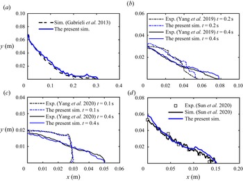
We validate the numerical approach by comparing with previous experiments and simulations for different initial conditions (Gabrieli et al. Reference Gabrieli, Artoni, Santomaso and Cola2013; Yang et al. Reference Yang, Jing, Kwok and Sobral2019, Reference Yang, Jing, Kwok and Sobral2020; Sun et al. Reference Sun, Zhang, Wang and Liu2020). The initial experimental set-up and its parameters are listed in table 1. For the simulation domain, the top surface is set to be a free-slip boundary, while no-slip conditions are applied along the bottom and  $x$-facing walls. In the spanwise
 $z$-direction, we employ periodic boundaries. A layer of particles with a uniform diameter is glued to the bottom to mimic the basal roughness. The size of the uniform rectangular grid is
 $\Delta x=\Delta y = \Delta z=d_{50}/20$. The granular column is prepared via the following steps. First, the particles are distributed randomly across the entire height of the lock region. The initial particle velocity is zero, and there is no initial contact. Second, the particles settle, with the friction coefficient
 $\mu _p$ varying from 0 to 1 to achieve different initial packing densities. Third, when all particles have settled in the lower part of the lock region,
 $\mu _p$ is adjusted back to the real value and the collapse is initiated. The front propagation in the experiment and simulation are compared in figure 2. We observe good qualitative and quantitative agreement for the time-dependent runout length and the free surface shape of the granular material, which we take as an indication that the computational model reproduces correctly the previous experimental and simulated behaviour for a cohesion/cohesionless collapse with different aspect ratios
 $a$, initial volume fractions
 $\varPhi$, and viscosity of ambient fluid
 $\nu _f$.
Parameters of the validation cases.

The time-dependent runout length and the free surface shape of the granular collapse for different validation cases. Panels (a,d) show the final surface shape.

For comparison, we run a case with identical parameters for the experiment of Yang et al. (Reference Yang, Jing, Kwok and Sobral2019), except that the dimensionless width of the tank is set to  $\tilde {W}=2.5$, in order to ensure that the spanwise domain size does not have a significant influence. It is found that the front propagation shows close agreement with that for the wider domain. So we set the computational domain width to
 $\tilde {W}=2.5$ in the parametric study to be described below. We remark that the present cohesive force implementation has been validated carefully by Vowinckel et al. (Reference Vowinckel, Withers, Luzzatto-Fegiz and Meiburg2019b) for the settling process of polydisperse sediments in quiescent fluid, and by Zhao et al. (Reference Zhao, Vowinckel, Hsu, Köllner, Bai and Meiburg2020, Reference Zhao, Pomes, Vowinckel, Hsu, Bai and Meiburg2021) for the flocculation of suspended particles in turbulence.
2.4. Computational set-up for cohesive simulations
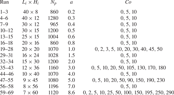
We consider a tank of size  $\tilde {L}\times \tilde {H}\times \tilde {W}=100\times 70\times 2.5$, with granular columns of
 $\tilde {L}_i\times \tilde {H}_i$ changing from
 $40\times 8$ to
 $7\times 60$. The corresponding aspect ratios
 $a$ increase from 0.2 to 8.6. The granular columns are composed of spherical particles of mean diameter
 $\tilde {d}_{50}=1$, with a weak polydispersity of
 $10\,\%$ standard deviation following a Gaussian distribution. A layer of particles with uniform diameter 0.5 is fixed at the bottom boundary to mimic basal roughness. We choose the coefficients of friction and restitution as
 $\mu _p=0.15$ (Joseph & Hunt Reference Joseph and Hunt2004) and
 $e_{dry}=0.97$ (Gondret, Lance & Petit Reference Gondret, Lance and Petit2002), corresponding to silicate materials. The size of the uniform rectangular grid is
 $\Delta x=\Delta y = \Delta z=\tilde {d}_{50}/20$. The initial granular columns are prepared similarly to the validation case, except that we do not change
 $\mu _p$ initially. The initial volume fraction is approximately 0.55, corresponding to a relatively loosely packed column (Rondon et al. Reference Rondon, Pouliquen and Aussillous2011). The Stokes number
 $St=12.79$ and the density ratio
 $r=1.6$ indicate that our cases are in the inertial regime. Cohesive sediments in the ocean typically have density of O(
 $10^{3}$ kg m
 $^{-3}$) and particle size of O(10
 $\mathrm {\mu }$m), which yield a smaller Stokes number that generally falls into the viscous regime (Pinzon & Cabrera Reference Pinzon and Cabrera2019; Vowinckel et al. Reference Vowinckel, Withers, Luzzatto-Fegiz and Meiburg2019b). Our simulations were motivated by the recent development of materials whose surface can be coated to give rise to cohesive bonds even for millimetric grain sizes (Jarray et al. Reference Jarray, Shi, Scheper, Habibi and Luding2019; Sauret et al. Reference Sauret, Gans, Gong, Pouliquen and Nicolas2019; Brunier-Coulin, Cuellar & Philippe Reference Brunier-Coulin, Cuellar and Philippe2020; Gans, Pouliquen & Nicolas Reference Gans, Pouliquen and Nicolas2020). In particular, Brunier-Coulin et al. (Reference Brunier-Coulin, Cuellar and Philippe2020) conducted submerged laboratory experiments with such particles, which resulted in cohesive granular flows in the inertial regime. The effects of cohesion can be observed more easily in this inertial regime, which prompted us to focus on this regime in the present investigation. We will discuss results from a total of 69 simulations focusing on the influence of
 $a$ and
 $Co$, whose parameters are listed in table 2. For convenience, the tilde symbol will be omitted henceforth.
Overview of the cohesive simulations conducted, and the associated parameter values. For all simulations,  $Ga=200$,
 $St=12.79$ and
 $r=1.6$.

3. Results
3.1. Observations of granular cohesive collapse
In order to set the stage for a subsequent quantitative analysis, we will initially discuss the overall qualitative properties of several representative simulations for shallow ( $a=1$) and tall (
 $a=8.6$) columns.
3.1.1. Collapse of shallow columns
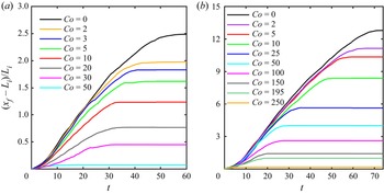
Figure 3(a) shows the evolution of the normalized front location  $(x_f-L_i)/L_i$ as a function of time. Here,
 $x_f$ denotes the location of the rightmost particle centre. Previous investigations (Meruane, Tamburrino & Roche Reference Meruane, Tamburrino and Roche2010; Lee et al. Reference Lee, Huang and Yu2018) had observed that the collapse of submerged, loosely packed, non-cohesive granular columns proceeds through three distinct stages: the acceleration or collapse stage, the constant front velocity stage, and the deceleration stage. Figure 3(a) demonstrates that these three stages also exist for cohesive granular collapse, and that the front velocity decreases monotonically as the cohesive force increases.
Evolution of the runout distance for: (a) shallow columns with aspect ratio  $a=1$ and cohesive numbers
 $Co=0$ to 50; (b) tall columns with aspect ratio
 $a=8.6$ and cohesive numbers
 $Co=0$ to 250. The collapse proceeds through distinct acceleration, constant-velocity and deceleration stages.

Snapshots of the magnitude of the angular and translational particle velocities,  $\|\boldsymbol {u}_{p}\|$ and
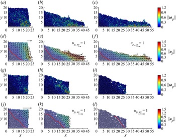
 $\|\boldsymbol \omega _p\|$, are shown in figure 4. Figures 4(d,j) show that the magnitude of the velocity vectors in the
 $x$- and
 $y$-directions remains very small in the lower left corner of the columns, which reflects the fact that the particles remain approximately at rest in this region. They demonstrate that for both cohesive and non-cohesive (Sun et al. Reference Sun, Zhang, Wang and Liu2020) columns, during the acceleration stage, particles near the upper right corner slide down along an inclined failure surface (indicated by a red line in figures 4d,j). The failure surface is defined as the contour where
 $\|\boldsymbol {u}_p\| = 0.05\|\boldsymbol {u}_p\|_{max}$ (Lacaze & Kerswell Reference Lacaze and Kerswell2009), with
 $\|\boldsymbol {u}_p\|_{max}$ denoting the maximum translational velocity at the same time. By comparing figures 4(d,j), we note that cohesive forces corresponding to
 $Co=30$ elevate the location of the failure surface, resulting in the growth of the region of stationary particles in the lower left corner. Interestingly, the angular velocity of the particles remains quite small near the failure surface (cf. figures 4a,b,g,h), which indicates that the particles slide, rather than roll, past each other (Xu et al. Reference Xu, Dong and Ding2019). The cohesive forces do not modify significantly the angular velocity field of the particles.
Evolution of granular collapse for  $a=1$ and
 $Co=0$ and 30, for (a,d,g,j)
 $t=5$, (b,e,h,k)
 $t=20$, and (c, f,i,l)
 $t=30$. (a–c) Magnitude of the angular velocity
 $\|\boldsymbol \omega _p\|$ for
 $Co=0$. (d–f) Magnitude of the translational velocity
 $\|\boldsymbol {u}_p\|$ for
 $Co=0$. (g–i) Magnitude of the angular velocity
 $\|\boldsymbol \omega _p\|$ for
 $Co=30$. (j–l) Magnitude of the translational velocity
 $\|\boldsymbol {u}_p\|$ for
 $Co=30$. The red lines indicate the location of the failure surface. The black arrows represent vectors of the average particle velocity.

During the constant-velocity stage, particles slide continuously towards the front of the collapsing column (figures 4e,k). The cohesive forces prevent particles from detaching and result in the formation of aggregates. We remark that the cohesive forces furthermore cause small fluctuations of the front velocity during the approximately constant-velocity stage; cf. figure 3(a). During the deceleration stage, the granular flow becomes increasingly shallow, and it forms a thin tip in the frontal region. For  $Co=30$, the final deposit profile is shorter and thicker; cf. figures 4( f,l). The surface of the deposit takes a rougher and more irregular shape, reminiscent of observations for dry cohesive granular collapse by Langlois et al. (Reference Langlois, Quiquerez and Allemand2015). Furthermore, Figure 3(a) indicates that cohesive flows decelerate more abruptly, compared to the non-cohesive case. For
 $Co=50$, the cohesive force is sufficiently large so that the column no longer collapses. This is similar qualitatively to previous experimental and numerical observations for dry cohesive granular collapse (Artoni et al. Reference Artoni, Santomaso, Gabrieli, Tono and Cola2013; Langlois et al. Reference Langlois, Quiquerez and Allemand2015; Santomaso et al. Reference Santomaso, Volpato and Gabrieli2018).
3.1.2. Collapse of tall columns
Similar to shallow columns, the collapse of tall columns also displays an initial acceleration stage, a subsequent constant-velocity stage, and finally a deceleration stage; cf. figure 3(b). However, during the acceleration stage, the influence of  $Co$ is much less pronounced than for shallow columns. This is a consequence of the fact that the early stages of the collapse of tall columns are dominated by the nearly solid-body free-fall motion of the upper column sections, which is largely unaffected by cohesive forces. Similarly to shallow columns, the runout distance for tall columns decreases with increasing
 $Co$.
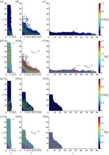
Images of the angular and translational velocity magnitudes in figure 5 demonstrate the early solid-body free-fall motion of the upper column sections over a wide  $Co$ range (Jing et al. Reference Jing, Yang, Kwok and Sobral2018). Only in the bottom left corner do the particles remain at rest, e.g. figures 5(d,j). For
 $Co=0$, most of the lower section of the column moves towards the right and forms a current head. In this region, the translational particle velocity
 $\|\boldsymbol {u}_p\|$ has a strong vertical gradient from the upper surface to the interior. We also notice that the rotational particle motion near the failure surface is much more pronounced than for shallow columns. For
 $Co>100$, the cohesive forces slow down the horizontal spreading of the particles near the bottom significantly (figure 5k), which in turn decelerates the free-fall motion of the upper sections, so that the acceleration stage terminates earlier (figure 3b). Furthermore, figure 5 demonstrates that for larger
 $Co$ values, the duration of the constant-velocity stage decreases gradually. While a number of individual particles detach from the collapsing column in the cohesionless case (figures 5b,e), the cohesive forces largely prevent the detachment of individual particles; cf. figures 5(h,k).
Sequences of snapshots for  $a=8.6$, with
 $Co=0$ and 100, at different times, for (a,d,g,j)
 $t=5$, (b,e,h,k)
 $t=20$, and (c, f,i,l)
 $t=60$. (a–c) Magnitude of the angular velocity
 $\|\boldsymbol \omega _p\|$ for
 $Co=0$. (d–f) Magnitude of the translational velocity
 $\|\boldsymbol {u}_p\|$ for
 $Co=0$. (g–i) Magnitude of the angular velocity
 $\|\boldsymbol \omega _p\|$ for
 $Co=100$. (j–l) Magnitude of the translational velocity
 $\|\boldsymbol {u}_p\|$ for
 $Co=100$. The red lines indicate the location of the failure surface. The black arrows represent vectors of the average particle velocity. In (l), the particle velocity is zero.

3.2. Front velocity and internal velocity profile
3.2.1. Front velocity
We now proceed to describe the quantitative dependence of the quasi-steady front velocity  $u_f$ on
 $Co$, for different aspect ratios
 $a$. With
 $u_{f0}$ denoting the quasi-steady front velocity for
 $Co=0$, Lee et al. (Reference Lee, Huang and Yu2018) observed that
 $u_{f0}/\sqrt {g'L_i}$ depends on the aspect ratio in a piecewise power-law fashion. Specifically, for
 $a<3$ they found
 $u_{f0}/\sqrt {g'L_i}\sim a^{{1}/{2}}$, while for
 $a>3$ they obtained
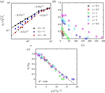
 $u_{f0}/\sqrt {g'L_i} \sim a^{{1}/{3}}$. Figure 6(a) shows our current simulation results for the normalized front velocity as a function of the aspect ratio
 $a$ for different
 $Co$ values. For
 $Co=0$, we find that it is well approximated by the power laws
 \begin{equation} u_{f0}/\sqrt{g'L_i}=\left\{\begin{array}{@{}ll} 0.27a^{{1}/{2}}, & a\leq 3,\\ 0.39a^{{1}/{4}}, & a\geq 3. \end{array} \right. \end{equation}
For  $a\le 3$ our exponent is identical to that of Lee et al. (Reference Lee, Huang and Yu2018), while for
 $a\ge 3$ it is somewhat smaller than the value found by those authors. We suspect that this discrepancy may be due to differences in the simulation approach, such as the details of the particle collision model. Also, note that Lee et al. (Reference Lee, Huang and Yu2018) employ a continuum two-phase flow model. In the presence of moderate cohesive forces, the front velocity continues to follow a power-law dependence, although for all but the largest aspect ratios the front velocity is somewhat smaller than for the cohesionless case. For those large aspect ratios, gravitational forces dominate over moderate cohesive forces during the early stages, so that cohesion does not slow down significantly the spreading of the collapsing column. This is confirmed by figure 6(b), which presents the normalized spreading velocity
 $u_f/\sqrt {g'L_i}$ as a function of
 $Co$ for different aspect ratios
 $a$. It shows that for
 $a>3$, the effect of cohesion is felt only above a certain value of
 $Co$.
(a) Normalized quasi-steady front velocity  $u_f/\sqrt {g'L_i}$ as a function of the aspect ratio
 $a$ for different cohesive numbers
 $Co$. The solid and dashed lines represent power-law fits for cases
 $Co=0$ and
 $Co=10$, respectively. The black and blue data points are nearly identical to the red data points for
 $a=5$ and 8.6. (b) Normalized quasi-steady front velocity
 $u_f/\sqrt {g'L_i}$ as a function of the cohesive number
 $Co$ for different aspect ratios
 $a$. (c) Ratio
 $u_f/u_{f0}$ as a function of
 $Co^{{2}/{3}}a^{-{1}/{2}}$. The dashed line represents
 $u_f/u_{f0}=1-0.07\,Co^{{2}/{3}}a^{-{1}/{2}}$.

We now focus on the ratio  $u_f/u_{f0}$, where
 $u_{f0}$ is calculated by (3.1). Close inspection of the data suggests that
 $u_f/u_{f0}$ can be well approximated by a power law of the form
 $Co^{\lambda _1}a^{\lambda _2}$. Specifically, the relationship
 $u_f/u_{f0} = 1- 0.07\,Co^{{2}/{3}}a^{-{1}/{2}}$ results in the coefficient of determination (‘goodness of fit’)
 $R^{2}=0.96$ as shown in figure 6(c). By combining this expression with (3.1), we obtain as empirical fit for the normalized front velocity
 \begin{equation} u_f/\sqrt{g'L_i}=(1-0.07\,Co^{{2}/{3}}a^{-{1}/{2}})\times\left\{\begin{array}{@{}ll} 0.27a^{{1}/{2}}, & a\leq 3,\\ 0.39a^{{1}/{4}}, & a\geq 3. \end{array} \right.\end{equation}
3.2.2. Internal velocity profile
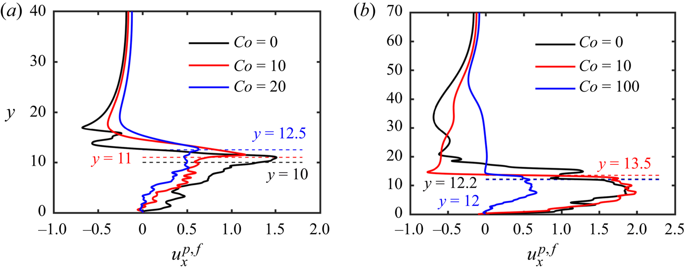
Figure 7(a) shows the velocity profile  $u^{p,f}_x(y)$, for different
 $Co$ values and
 $a=1$, at location
 $x=20$ and time
 $t=20$. Here,
 $u^{p,f}_x(y)$ is the horizontal fluid velocity at locations occupied by fluid, and the horizontal velocity of the particle centre at locations inside a particle. Furthermore,
 $u^{p,f}_x(y)$ represents the
 $z$-averaged value, and it increases from approximately zero at the lower wall to a maximum near the upper particle boundary. Cohesion reduces the propagation velocity of the fluid–particle mixture, which is consistent with our earlier observations regarding the front velocity. Immediately above the particles, the fluid moves even faster than the mixture. As
 $y$ increases further, the velocity profile exhibits a sharp transition to the leftward counterflow in the upper part of the domain.
(a) Plots of  $u^{p,f}_x(y)$ at location
 $x=20$ and time
 $t=20$, for aspect ratio
 $a=1$ and various
 $Co$ values. (b) Plots of
 $u^{p,f}_x(y)$ at
 $x=15$ and
 $t=20$, for aspect ratio
 $a=8.6$ and different
 $Co$ values. The dashed lines indicate the location of the upper boundary of the particles.

For  $a=8.6$, the maximum of
 $u^{p,f}_x(y)$ occurs inside the fluid–particle mixture, and the uppermost layer of this mixture is already retarded by the counterflow; cf. figure 7(b). We note that cohesionless collapses give rise to small-scale fluctuations of
 $u^{p,f}_x(y)$ in the fluid region above, due to the influence of detached particles.
3.3. Runout distance, final deposit height and deposit morphology
3.3.1. Runout distance and final deposit height
We now shift our focus to the final runout distance  $l_f$ and the maximum deposit height
 $h_f$. These two quantities were also employed by Bougouin & Lacaze (Reference Bougouin and Lacaze2018) in order to characterize the deposit. Several previous studies of submerged non-cohesive granular collapses found their values for
 $Co=0$, i.e.
 $l_{f0}$ and
 $h_{f0}$, to depend on the aspect ratio
 $a$ in a piecewise power-law fashion (Bougouin & Lacaze Reference Bougouin and Lacaze2018; Jing et al. Reference Jing, Yang, Kwok and Sobral2018; Lee et al. Reference Lee, Huang and Yu2018).
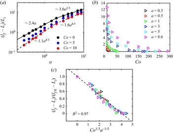
Figure 8(a) shows current simulation results for the normalized runout distance  $(l_f-L_i)/L_i$ as a function of the aspect ratio
 $a$, for different
 $Co$ values. Bougouin & Lacaze (Reference Bougouin and Lacaze2018) as well as Lee et al. (Reference Lee, Huang and Yu2018) observed that for cohesionless collapses with
 $a<2\unicode{x2013}3$, this normalized runout distance varies linearly with the aspect ratio. On the other hand, for
 $a>2\unicode{x2013}3$, they found
 $(l_{f0}-L_i)/L_i\sim \lambda _3a^{\lambda _4}$, where
 $\lambda _4$ changes from 0.56 to 0.67, depending on other parameters such as the particle size and density. The present simulation results show that for
 $Co=0$, the normalized runout distance behaves as
 \begin{equation} (l_{f0}-L_i)/L_i=\left\{\begin{array}{@{}ll} 2.4a, & a\leq 2,\\ 3a^{{2}/{3}}, & a\geq 2, \end{array} \right. \end{equation}
which is consistent with the earlier findings. In the presence of cohesive forces, the normalized runout distance decreases gradually for a given aspect ratio, as can be seen in figures 8(a,b). A similar trend was also observed for dry cohesive granular collapses by Langlois et al. (Reference Langlois, Quiquerez and Allemand2015), Santomaso et al. (Reference Santomaso, Volpato and Gabrieli2018) and Artoni et al. (Reference Artoni, Santomaso, Gabrieli, Tono and Cola2013).
(a) Normalized runout distance  $(l_f-L_i)/L_i$ as a function of the aspect ratio
 $a$ for different
 $Co$ values. The solid and dashed lines represent power-law fittings for
 $Co=0$ and
 $Co=10$, respectively. (b) Normalized runout distance
 $(l_f-L_i)/L_i$ as a function of the cohesive number
 $Co$ for different aspect ratios
 $a$. (c) Normalized runout distance
 $(l_f-L_i)/(l_{f0}-L_i)$ as a function of
 $Co^{{1}/{3}}a^{-{1}/{5}}$. The dashed line represents
 $(l_f-L_i)/(l_{f0}-L_i)=1-0.25\,Co^{{1}/{3}}a^{-{1}/{5}}$.

In order to obtain the quantitative dependence of the runout distance on  $Co$, we follow the strategy that had been successful for the front velocity, and normalize the runout distance as
 $(l_f-L_i)/(l_{f0}-L_i)$. The simulation data are well captured (
 $R^{2}=0.97$) by
 $(l_f-L_i)/(l_{f0}-L_i)=1-0.25\,Co^{{1}/{3}}a^{-{1}/{5}}$, as shown in figure 8(c). By combining this expression with (3.3) for the cohesionless runout length
 $l_{f0}$, we obtain as empirical fit for the runout distance,
 \begin{equation} (l_f-L_i)/L_i=(1-0.25\,Co^{{1}/{3}}a^{-{1}/{5}})\times\left\{ \begin{array}{@{}ll} 2.4a, & a\leq 2,\\ 3a^{{2}/{3}}, & a\geq 2. \end{array} \right.\end{equation}
Equation (3.4) shows that  $Co$ and
 $a$ affect the front velocity and runout distance in corresponding fashion, with larger
 $Co$ reducing the runout distance in a way that is more pronounced for smaller
 $a$. Note that the scaling law
 $Co^{{1}/{3}}$ in (3.4) is similar to
 $Bo^{-{1}/{3}}$ in Artoni et al. (Reference Artoni, Santomaso, Gabrieli, Tono and Cola2013). This is because the cohesive number
 $Co$ is the reciprocal of the bond number
 $Bo$, which is calculated as the gravitational force divided by the capillary (or cohesive) force. This indicates the quantitative similarity of the effect of cohesive force between dry and submerged cases.
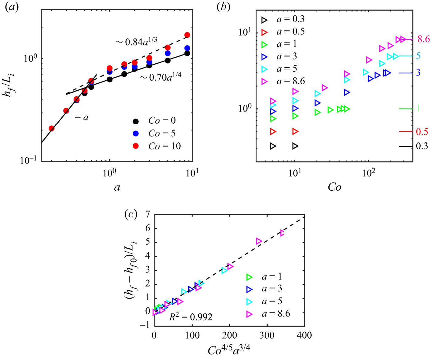
Simulation results for the dependence of the normalized final deposit height  $h_f/L_i$ on the aspect ratio
 $a$ are presented in figure 9(a). For
 $Co=0$, we find that
 $h_{f0}/L_i$ varies linearly with
 $a$ for small
 $a$. Note that in this region, the black and blue data points coincide with the red data points, which indicates that for small aspect ratios, the deposit height does not depend on
 $Co$. This reflects the fact that for these small aspect ratios, the leftmost part of the column top does not participate in the collapse, so that a trapezoidal deposit shape evolves, as was also observed by Bougouin & Lacaze (Reference Bougouin and Lacaze2018) and Lee et al. (Reference Lee, Huang and Yu2018). For larger values of
 $a$, we find that for non-cohesive collapses,
 $h_{f0}/L_i$ varies as
 \begin{equation} h_{f0}/L_i=\left\{\begin{array}{@{}ll} a, & a\leq 0.53,\\ 0.7a^{{1}/{4}}, & a\geq 0.53. \end{array} \right. \end{equation}
This is reasonably close to the observations of Bougouin & Lacaze (Reference Bougouin and Lacaze2018) and Lee et al. (Reference Lee, Huang and Yu2018), who found that for non-cohesive collapses, the transitional value of  $a$ between the regimes varies from 0.6 to 0.75, while the exponent ranges from 0.33 to 0.48. For larger aspect ratios
 $a$, the final deposit height is seen to increase with
 $Co$; cf. figure 9(a). The transitional value of
 $a$ between the regimes increases slightly with
 $Co$, which indicates that in the presence of cohesive forces, the final deposit profile maintains a trapezoidal shape for larger aspect ratios. Figure 9(b) confirms that for sufficiently large cohesive forces, the leftmost section of the column does not collapse, so that
 $h_f/L_i=a$.
(a) Normalized final deposit height  $h_f/L_i$ as a function of the aspect ratio
 $a$ for different
 $Co$ values. The solid and dashed lines represent power-law fittings for
 $Co=0$ and 10, respectively. (b) Normalized final deposit height
 $h_f/L_i$ as a function of the cohesive number
 $Co$ for different aspect ratios. The tick marks along the right vertical axis indicate
 $h_f/L_i=a$. (c) Plots of
 $(h_f-h_{f0})/L_i$ as a function of
 $Co^{{4}/{5}}a^{{3}/{4}}$. The dashed line represents
 $(h_f-h_{f0})/L_i=0.02\,Co^{{4}/{5}}a^{{3}/{4}}$.

In order to quantify the dependence of the final deposit height on  $Co$, we focus on those collapses that affect the entire top layer of the original column, so that
 $h_f/L_i< a$, i.e. the maximum final deposit height is lower than the original column height. Figure 9(b) shows that for these cases,
 $h_f/L_i$ varies with both
 $Co$ and
 $a$. The simulation data are well captured (
 $R^{2}=0.992$) by the relationship
 $(h_f-h_{f0})/L_i=0.02\,Co^{{4}/{5}}a^{{3}/{4}}$ shown in figure 9(c). Together with (3.5) for
 $h_{f0}$, we thus obtain the empirical fit
 \begin{equation} h_f/L_i=\left\{\begin{array}{@{}ll} 0.02Co^{{4}/{5}}a^{{3}/{4}}+0.7a^{{1}/{4}}, & a\geq 0.53\ \mathrm{and}\ Co^{{4}/{5}}\leq 50a^{{1}/{4}}-35a^{-{1}/{2}},\\ a, & \mathrm{otherwise}. \end{array} \right. \end{equation}
Equation (3.6) indicates that the increase of the final deposit height due to cohesion is more pronounced for larger aspect ratios  $a$.
3.3.2. Deposit morphology
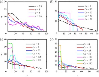
Figure 10(a) shows the final deposit profiles of non-cohesive collapse simulations for different values of the aspect ratio  $a$. For
 $a=0.3$, the profile has a trapezoidal shape, with a flat top towards the left that has essentially remained unaffected by the collapse process, and an approximately uniform slope towards the right. As
 $a$ increases, the top of the sloping section moves closer and closer to the left wall, and between
 $a=1$ and 3, the deposit has a nearly triangular shape. For
 $a=8.6$, the final deposit shape resembles a ‘Mexican hat’, characterized by an approximately flat outer region with steep central cone. These observations are consistent with previous findings (Rondon et al. Reference Rondon, Pouliquen and Aussillous2011; Lee et al. Reference Lee, Huang and Yu2018).
Deposit profiles for different aspect ratios  $a$ and cohesive numbers
 $Co$: (a)
 $Co=0$, (b)
 $a=1$, (c)
 $a=3$, and (d)
 $a=8.6$.

The presence of cohesive forces modifies the surface shape of the final deposit significantly; cf. figures 10(b–d). The formation of larger aggregates during the collapse process causes the surface to be rougher than for cohesionless collapses, and the steepness of the final profile increases with  $Co$. For moderate values of
 $Co$, both convex and concave deposit surfaces can form, while sufficiently strong cohesive forces suppress the collapse nearly entirely.
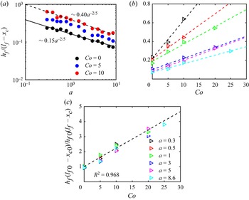
For deposits with a trapezoidal or triangular shape, we evaluate the magnitude of the uniform slope as  $h_f/(l_f-x_c)$, where
 $x_c$ denotes the leftmost point on the uniform slope. Figure 11(a) shows the slope
 $h_f/(l_f-x_c)$ as a function of the aspect ratio for different values of
 $Co$. Similar to the runout distance and the final deposit height, the surface slope has a piecewise power-law dependence on
 $a$. For
 $Co=0$, the best fit is given by
 \begin{equation} h_{f0}/(l_{f0}-x_{c0})=0.15a^{-{2}/{5}}, \end{equation}
where  $x_{c0}$ denotes the value for
 $Co=0$. The critical value of
 $a$ for the transition of the piecewise function is 1. While figure 11(a) indicates that the slope increases with
 $Co$, it also suggests that the exponent of the power law may be sensitive to the exact value of
 $Co$.
(a) The deposit surface slope  $h_f/(l_f-x_c)$ as a function of
 $a$ for different values of
 $Co$. The solid and dashed lines represent power-law fittings for the cases
 $Co=0$ and 10, respectively. (b) The deposit surface slope
 $h_f/(l_f-x_c)$ as a function of
 $Co$ for different values of
 $a$. The dashed lines indicate linear fittings. (c) Normalized slope
 ${h_f(l_{f0}-x_{c0})}/{h_{f0}(l_f-x_c)}$ as a function of
 $Co$. The dashed line represents
 ${h_f(l_{f0}-x_{c0})}/{h_{f0}(l_f-x_c)}=1+0.12\,Co$.

Figure 11(b) presents the surface slope as a function of  $Co$ for moderate cohesive forces that do not suppress the collapse:
 $h_f/(l_f-x_c)$ increases approximately linearly with
 $Co$, and its dependence on
 $Co$ becomes weaker for larger aspect ratios. If we normalize
 $h_f/(l_f-x_c)$ by the cohesionless slope
 $h_{f0}/(l_{f0}-x_{c0})$, then figure 11(c) suggests that this normalized slope varies with
 $Co$ approximately as
 $1+0.12\,Co$, with
 $R^{2}=0.965$. By combining this relationship with (3.7), we obtain the slope of trapezoidal and triangular deposits:
 \begin{equation} h_f/(l_f-x_c)=0.15(1+0.12\,Co)a^{-{2}/{5}}. \end{equation}
3.4. Energy budget
In the following, we analyse the temporal evolution of the various particle and fluid energy components (Vowinckel et al. Reference Vowinckel, Withers, Luzzatto-Fegiz and Meiburg2019b) during the submerged granular collapse, for different cohesive force strengths. The potential energy stored initially in the granular column represents the source that drives the collapse. This energy is converted into kinetic energy of the particles and fluid, potential energy of the fluid, and elastic potential energy stored at the contact points between particles. Energy is dissipated primarily due to fluid viscosity, particle–particle friction, and inelastic collisions. Here, we focus on the dominant components of the energy budget, which are given by the potential and kinetic energy of the particles,  $E_p$ and
 $E^{p}_k$, and the kinetic energy of the fluid,
 $E^{f}_k$. These are defined, respectively, as
 $$\begin{gather} E_p(t)=\sum_{i=1}^{N_p}(\rho_p-\rho_f)V_{p,i}gh_{c,i}, \end{gather}$$
 $$\begin{gather}E^{p}_k(t)=\frac{1}{2}\sum_{i=1}^{N_p}m_{p,i}\,\|\boldsymbol{u}_{p,i}\|^{2}, \end{gather}$$
 $$\begin{gather}E^{f}_k(t)=\frac{1}{2}V_{fc}\sum_{i=1}^{N_{fc}}\rho_f(\phi_{fcu} u^{2}+\phi_{fcv}v^{2}+\phi_{fcw}w^{2}), \end{gather}$$
where  $V_{p,i}$ and
 $h_{c,i}$ denote the volume and centre height of particle
 $i$, respectively. We note that we use
 $(\rho _p-\rho _f)$ because it is associated with the available potential energy that can be released by a particle. Also,
 $V_{fc}$ is the volume of a grid cell,
 $N_{fc}$ is the total number of grid cells, and
 $\phi _{fcu}$,
 $\phi _{fcv}$ and
 $\phi _{fcw}$ represent the fluid volume fractions in the grid cells for velocity components
 $u$,
 $v$ and
 $w$, respectively. Note that these volume fractions can be different for the different velocity components, due to the staggered grid approach employed in our simulations. The rotational kinetic energy of the particles is small enough that we can neglect it (Jing et al. Reference Jing, Yang, Kwok and Sobral2018). We remark that we keep track of the separate kinetic energy components associated with the
 $u$- and
 $v$-velocities of the particles (
 $E^{p}_{kx}$ and
 $E^{p}_{ky}$) and the fluid (
 $E^{f}_{kx}$ and
 $E^{f}_{ky}$), so that we can distinguish how kinetic energy associated with the vertical falling motion is redirected in the horizontal direction during the collapse process:
 $$\begin{gather} E^{p}_{kx}(t)=\frac{1}{2}\sum_{i=1}^{N_p}m_{p,i}u^{2}_{p,i}, \end{gather}$$
 $$\begin{gather}E^{p}_{ky}(t)=\frac{1}{2}\sum_{i=1}^{N_p}m_{p,i}v^{2}_{p,i}, \end{gather}$$
 $$\begin{gather}E^{f}_{kx}(t)=\frac{1}{2}V_{fc}\sum_{i=1}^{N_{fc}}\rho_f\phi_{fcu} u^{2}, \end{gather}$$
 $$\begin{gather}E^{f}_{ky}(t)=\frac{1}{2}V_{fc}\sum_{i=1}^{N_{fc}}\rho_f\phi_{fcv}v^{2}. \end{gather}$$
We note that the partial kinetic energy associated with the  $w$-velocity component is negligible (Jing et al. Reference Jing, Yang, Kwok and Sobral2018).
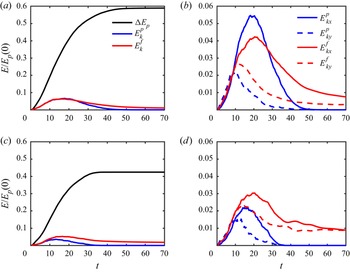
Figure 12 shows the time history of the energy budget for different  $Co$ values and
 $a=1$. Here, we normalize all energy components by the initial available potential energy of the particles,
 $E_p(0)$;
 $\Delta E_p=E_p(0)-E_p(t)$ indicates the amount of potential energy that has been released by the particles up to time
 $t$. The presence of cohesive forces reduces significantly the amount of available potential energy released by the particles, as shown in figure 12(c). This reflects the fact that cohesive collapses result in shorter runouts and thicker deposits, so that they retain more of their potential energy; cf. figure 5. We note that the kinetic energy of the particles decreases much more strongly than that of the fluid, compared to the cohesionless case, as the cohesive forces prevent the particles from moving freely; cf. figures 12(b,d). Interestingly, the fluid retains a significant amount of kinetic energy long after the particles have come to rest. Figures 12(b,d) show the evolution of the kinetic energy components associated with the
 $u$- and
 $v$-velocity components for a shallow column, with
 $Co=0$ and 10, respectively. We notice that the peak kinetic energy values are reduced greatly by the cohesive forces, and much more so for the horizontal component than for the vertical one, which suggests that for stronger cohesive forces, less and less of the particle kinetic energy associated with the free fall is redirected in the horizontal direction. The
 $x$-components of the particle and fluid kinetic energies also peak earlier for larger
 $Co$ values, reflecting an earlier onset of the deceleration stage.
Time history of the largest components of the energy budget, for different cohesive numbers  $Co$ and
 $a=1$: (a,b)
 $Co=0$, (c,d)
 $Co=10$.

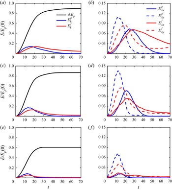
Figure 13 shows corresponding energy conversion results for tall columns with  $a=8.6$. In the presence of cohesive forces, the sediment gives up a substantially smaller fraction of its initial potential energy, e.g. about
 $60\,\%$ and
 $90\,\%$ for
 $Co=100$ and 0, respectively. Interestingly, while for moderate cohesive forces the kinetic energy peak of the fluid remains approximately unchanged, the peak of the particle kinetic energy increases compared to the cohesionless case; cf. figure 13(c). Only for strongly cohesive collapses does the peak of the particle kinetic energy decrease; cf. figure 13(e). The explanation for the increase in the particle kinetic energy under moderate cohesive forces can be found in figures 13(b,d), which show that it is primarily the kinetic energy component associated with the vertical particle velocity that increases under mild cohesion. Cohesion holds the upper section of the column together during its free fall, which allows it to reach a larger vertical velocity than for the cohesionless case. For large cohesive forces, on the other hand, the entire free-fall motion slows down much earlier, so that the particles never acquire a large vertical velocity.
Time history of various energy components for different cohesive numbers  $Co$ when
 $a=8.6$: (a,b)
 $Co=0$, (c,d)
 $Co=10$, and (e, f)
 $Co=100$.

3.5. Internal structure of the deposit
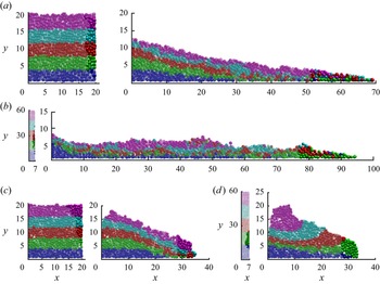
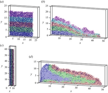
In figure 14, we employ different colours in order to mark five horizontal particle layers in the initial column, which we then track until the end of the collapse process for different  $Co$. We also identify the 100 particles that have travelled the farthest at the end of the collapse process. Both the initial and final locations of these particles are then marked in opaque colour. For both cohesive and cohesionless columns with
 $a=1$, the layers stay mostly intact towards the left of the final deposit, whereas there tends to be more mixing towards the tip of the deposit on the right. The particles initially at the base of the column are slowed down by bottom friction, whereas those initially at the top are somewhat retarded by the ambient counterflow. The particles that travel the farthest are mostly from the second- and third-highest layers. These particles all originate in a thin vertical slice at the right of the initial column that extends over nearly the entire height of the column for
 $Co=0$ (cf. figure 14a), and from the top to about
 $3/4$ of the way down for
 $Co=20$ (cf. figure 14c).
The internal structure of the final deposit for different  $Co$ values and aspect ratios. Colour indicates the original horizontal particle layers. The 100 particles nearest to the front of the final deposit and their initial locations are marked in opaque colour. Values are: (a)
 $Co=0$ and
 $a=1$; (b)
 $Co=0$ and
 $a=8.6$; (c)
 $Co=20$ and
 $a=1$; (d)
 $Co=50$ and
 $a=8.6$. (See also supplementary movies 1–4, available at https://doi.org/10.1017/jfm.2022.404.)

For collapses with  $a=8.6$, on the other hand, there is more pronounced mixing between the layers for the non-cohesive case, whereas for
 $Co=50$, the layers tend to retain their identities. Interestingly, the particles that travel the farthest now originate in the second layer from the bottom and in a thin vertical slice at the right of the initial column. For
 $a=8.6$ and
 $Co=0$ (cf. figure 14b), this thin slice along the right edge of the initial column does not extend all the way to the top, because the particles near the very top move down primarily, rather than towards the right. For
 $Co=50$ (cf. figure 14d), the slice is somewhat thicker, but it occupies only about
 $1/6$ of the column height.
3.6. Formation and persistence of aggregates in the interior of the granular collapse
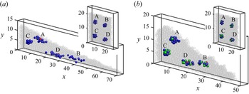
In order to demonstrate the formation and persistence of aggregates in the interior of the granular collapse, figure 15 focuses on collapses with aspect ratio  $a=1$, and compares the two cases
 $Co=0$ and 10. The initial configurations are identical, and the figure tracks the same four distinct particles A, B, C and D (marked in red) for both flows. For each of these four particles, we furthermore keep track of those neighbours (marked in blue) that are initially separated from them by a distance smaller than 0.5 unit lengths. For
 $Co=10$, if these neighbouring particles are sufficiently close to A, B, C or D to form a cohesive bond with them at the initial time, they are marked in green. Figures 15(a,b) show the initial and final locations of all these neighbours. Particles A and C and their neighbours travel a relatively short distance during the collapse, so that they remain close to their initial neighbours for both
 $Co=0$ and
 $Co=10$. On the other hand, particles B and D travel much larger distances, and their neighbours become much more separated from each other during the collapse for
 $Co=0$ as compared to
 $Co=10$. This demonstrates that for
 $Co=10$, the cohesive forces result in the formation and persistence of aggregates of primary particles that tend to remain close to each other throughout the evolution of the flow.
The evolution of four particle clusters, each of which is initially centred around a red particle, for  $a=1$, with (a)
 $Co=0$, and (b)
 $Co=10$. At time
 $t=0$, the particle clusters are identical for both simulations. Those neighbours that initially have a cohesive bond with the red particle are shown in green. The initial clusters remain more compact for
 $Co=10$, whereas they become more disperse for
 $Co=0$. (See also supplementary movies 5 and 6.)

In order to quantify the tendency of aggregates to persist, we now introduce an  $x,y$-grid with uniform spacing of 1. For each grid point, we consider the group of particles whose centres are initially located within a
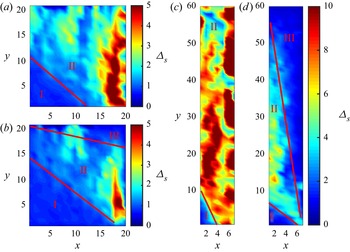
 $2 \times 2$-cell centred around this grid point. We then take the locations of this group of particles at the final time, find their centre of mass, and evaluate the average distance
 $\varDelta _s$ of the particles in this group from their centre of mass at the final time. The value of
 $\varDelta _s$ is then assigned to the grid point. Contours of
 $\varDelta _s$, shown in figure 16, then provide a measure of the tendency of the particles to get separated from their initial neighbours in the course of the collapse process.
Contours of  $\varDelta _s$, which reflect the tendency of neighbouring particles to get separated from each other during the course of the collapse. The cohesive forces generally reduce this tendency. It also results in the generation of a region near the upper right corner of the column where neighbouring particles stay close to each other. Values are: (a)
 $a=1$ and
 $Co=0$; (b)
 $a=1$ and
 $Co=10$; (c)
 $a=8.6$ and
 $Co=0$; (d)
 $a=8.6$ and
 $Co=25$.

For both  $a=1$ and
 $a=8.6$, we find that, on average, cohesion reduces the tendency of particles to get separated from their initial neighbours. In the absence of cohesion (figures 16a,c), the initial columns can be divided into two zones. The zone boundaries are presented qualitatively by visualization. In zone I near the lower left corner of the column,
 $\varDelta _s \approx 0$ since the particles in this zone hardly move at all. In zone II, particles flow along the failure surface and tend to get separated from each other, which results in large values of
 $\varDelta _s$. The region near the right edge of zone II, whose particles we earlier observed to travel the farthest, has the largest values of
 $\varDelta _s$. The presence of cohesive forces gives rise to a new zone III towards the upper right, where neighbouring particles tend to stay close to each other and travel as aggregates; cf. figures 16(b,d). The previous study by Dizaji, Marshall & Grant (Reference Dizaji, Marshall and Grant2019) provides an explanation for this observation. Their simulation results indicate that cohesive particle aggregates tend to break up when sheared. As shown in figures 4, 5 and 16, the particles in zone II are subject to the largest velocity gradients in the direction perpendicular to the failure surface, so we expect the shear to promote the breakup of cohesive bonds between particles; cf. figure 18.
Figure 17 shows the averaged values of  $\varDelta _s$ for the initial column (written as
 $\bar \varDelta _s$) as a function of the cohesive number
 $Co$ for different aspect ratios
 $a$. Here,
 $\bar \varDelta _s$ has a larger value for smaller
 $Co$ and higher
 $a$ due to the longer separated distance between the initial neighbouring particles. The graph suggests that
 $\bar \varDelta _s$ depends on the cohesive number
 $Co$ in a power-law fashion. As we increase the aspect ratio
 $a$, the effect of cohesive number
 $Co$ is stronger, i.e.
 $\bar \varDelta _s \sim Co^{-{1}/{10}}$ when
 $a=0.3$, while
 $\bar \varDelta _s \sim Co^{-{1}/{2}}$ when
 $a=8.6$.
The averaged values of  $\varDelta _s$ for the initial column as a function of the cohesive number
 $Co$ for different aspect ratios
 $a$. The dashed lines are power-law fittings for
 $a=0.3$ and
 $a=8.6$. Larger cohesive forces tend to hold the cluster of particles together throughout the collapse of the column.

3.7. Cohesive and contact force bonds
We now proceed to analyse cohesive and contact force bonds from a more global perspective, for  $Co=10$ as well as
 $a=1$ and 8.6, respectively. For the initial time
 $t=0$, figures 18(a,c) indicate all cohesive bonds between individual particles by straight-line segments that connect the particle centres. Figures 18(b,d) show those of the initial cohesive bonds that have survived until the end of the collapse. We observe a few clear differences between the two aspect ratios. As discussed earlier, for
 $a=1$, the particles in the lower left corner hardly move at all, so that many of the initial cohesive bonds between them survive the entire collapse process. Near the left wall, and in the entire upper (pink) layer, quite a few of the bonds also survive, whereas this is not true for the lower sections of the deposit near the front. For the particles in that section, the collapse process destroys most of their initial cohesive bonds. For
 $a=8.6$, on the other hand, cohesive bonds survive primarily in a very small section in the lower left corner, and along the entire top layer of the deposit, including at the very front. For the entire interior section of the final deposit, almost all initial cohesive bonds are destroyed during the course of the collapse.
Cohesive bonds at the initial time for (a)  $a=1$,
 $Co=10$, and (c)
 $a=8.6$,
 $Co=25$. For the same two flows, (b,d) show those cohesive bonds that have stayed intact during the entire collapse process until the final time
 $t=60$. (See also supplementary movies 7 and 8.)

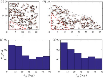
Figure 19 presents the strongest  $10\,\%$ of the instantaneous cohesive bonds at different times, for
 $a=1$ and
 $Co=10$. The strength of the bonds is indicated by the thickness of the corresponding line segments. The near-static area in the lower left corner (indicated by the dashed red lines) contains very few strong cohesive bonds, as the particle interaction in this region is dominated by direct contact forces. Outside this region, strong cohesive bonds can be found nearly anywhere in the flow, including near the free surface. Figures 19(c,d) indicate the directional distribution of the cohesive bonds, by showing the number
 $N_{cb}(\theta _{cb})$ of cohesive bonds whose angle
 $\theta _{cb}$ with the horizontal falls into a given range. For
 $t=5$, we find that the direction of the cohesive bonds is preferentially aligned with the horizontal. This tendency becomes somewhat more prominent throughout the collapse, as can be seen for
 $t=20$. This suggests that the cohesive bonds essentially cause a macroscopic stress tensor that counteracts the deformation tensor and hence limits the runout distance of the collapse.
(a,b) The strongest  $10\,\%$ of all cohesive bonds for
 $a=1$ and
 $Co=10$ at
 $t=5$ and 20, respectively. The thickness of the connecting lines denotes the strength of the cohesive force. The area in the lower left corner outlined by a dashed red triangle contains relatively few cohesive bonds, since direct contact forces dominate here. The black dashed lines indicate the instantaneous deposit shape. (c,d) The directional distribution of the cohesive bonds at
 $t=5$ and 20, respectively.

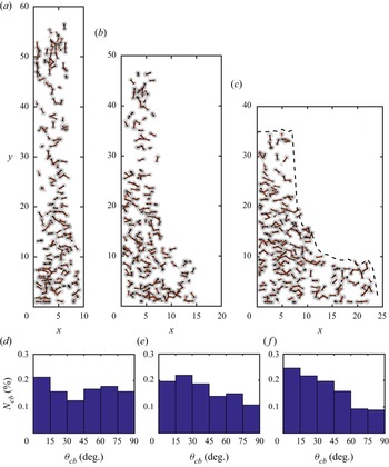
The situation is somewhat different for  $a=8.6$; cf. figure 20. Figure 20(d) indicates that the cohesive bonds are approximately uniformly distributed across all angles early on during the collapse. However, figure 20(a) shows strong local differences. The particles in the upper part of the column are in near free-fall motion, and the cohesive bonds point mainly in the vertical direction. In the lower part of the collapsing column, on the other hand, the particles move predominantly in the horizontal direction, and the cohesive bonds are aligned in this direction as well. As the upper part of the collapsing column slows its free fall and more particles are being redirected in the horizontal direction, the angular distribution of the cohesive bonds skews in this direction as well.
(a–c) The strongest  $10\,\%$ of the cohesive bonds for
 $a=8.6$ and
 $Co=10$ at
 $t=5$, 10 and 15, respectively. The thickness of the connecting lines denotes the magnitude of the cohesive forces. The dashed lines indicate the instantaneous deposit shape. (d–f) The directional distributions of the cohesive bonds at
 $t=5$, 10 and 15, respectively.

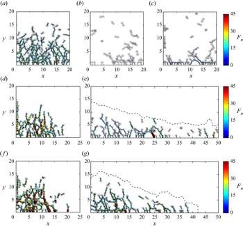
Figure 21 shows the strongest  $10\,\%$ of the normal direct contact forces between particles for
 $Co=0$ and 10, at different times. The force magnitude is again indicated by the thickness of the line segment. The initial configurations are identical for both
 $Co$ values, and as long as the particles are at rest, the normal contact forces are preferentially aligned with the vertical direction. They increase towards the bottom, as they have to support the weight of the overlying particles (Yang et al. Reference Yang, Jing, Kwok and Sobral2020); cf. figure 21(a). Shortly after the gate removal, the number of normal contact force connections is reduced greatly, due to the excess pore pressure that forms as the particle column begins to move and contracts (Rondon et al. Reference Rondon, Pouliquen and Aussillous2011; Vowinckel et al. Reference Vowinckel, Biegert, Luzzatto-Fegiz and Meiburg2019a; Yang et al. Reference Yang, Jing, Kwok and Sobral2020); cf. figures 21(b,c). During this stage, much of the particle weight is supported by dynamical pressure, rather than by direct contact force chains. At later times, branched-out contact force chains re-emerge, primarily towards the left and near the bottom wall, where particles come to rest and have to support the weight of the overlying grains once more; cf. figures 21(d, f). Near the upper surface, the particles move rapidly, so that particle–particle collisions can generate considerable contact forces. However, these local contact forces do not constitute part of a larger network; cf. figures 21(e,g).
The strongest  $10\,\%$ of the normal contact forces for
 $a=1$ and various
 $Co$ values at different times: (a)
 $t=0$ before the lock gate removal; (b)
 $Co=0$ and
 $t=0.5$; (c)
 $Co=10$ and
 $t=0.5$; (d)
 $Co=0$ and
 $t=5$; (e)
 $Co=0$ and
 $t=30$; ( f)
 $Co=10$ and
 $t=5$; (g)
 $Co=10$ and
 $t=30$. The thickness and colour of the contact segments denote the magnitude of the normal contact force. The dashed lines indicate the instantaneous deposit shape.

4. Summary and conclusions
We have analysed the submerged collapse of weakly polydisperse, loosely packed cohesive granular columns. Towards this end, we have employed fully coupled, grain-resolving direct numerical simulations. As the two dominant dimensionless parameters governing this problem, we focus on the influence of the aspect ratio  $a$ of the initial particle column, as well as a cohesive number
 $Co$ that provides the ratio of cohesive to gravitational forces acting on the particles. The simulations demonstrate that for both shallow and tall columns, the cohesive forces largely prevent the detachment of individual particles from the main body of the collapsing column. Furthermore, it reduces the front velocity, and it results in a shorter and thicker final deposit. We show that the effect of the cohesive force and the aspect ratio on the quasi-steady front velocity, the runout distance, and the final deposit height can be captured accurately across a broad range of
 $Co$ and
 $a$ values by piecewise power-law relationships.
The energy budget analysis shows that the presence of cohesive forces reduces significantly the amount of available potential energy released by the particles, due to the shorter runout distance and thicker final deposits. For shallow columns, the particles and fluid acquire less kinetic energy as  $Co$ increases. For tall columns, on the other hand, moderate cohesive forces increase the maximum particle kinetic energy since it accelerates the initial free fall of the upper column section. Only for larger cohesive forces does the peak kinetic energy of the particles decrease.
By tracking the individual particles, we obtain insight into the Lagrangian dynamics and mixing behaviour of the granular collapse. In general, the cohesive forces are seen to reduce the mixing of particles within the collapsing column. Furthermore, the simulations enable us to identify the region within the initial column from where those particles originate that travel the farthest. We find that for all aspect ratios and  $Co$ values, this region represents a narrow slice along the collapsing edge, although the vertical location of this slice varies with
 $Co$ and
 $a$. Bottom friction generally prevents the particles at the base of the column from travelling very far.
The simulations demonstrate clearly that larger cohesive forces tend to keep initial neighbour particles together throughout the evolution of the flow, i.e. they promote the formation of aggregates. Furthermore, the simulations provide complete information on the temporally and spatially evolving network of cohesive and direct contact force bonds. The normal contact forces are aligned primarily in the vertical direction, as they support the weight of the overlying particles. The cohesive bonds, on the other hand, adjust their preferred spatial orientation throughout the evolution of the collapse. They give rise to a net macroscopic stress tensor that counteracts the deformation tensor and hence slows the spreading of the advancing particle front.
Supplementary movies
Supplementary movies are available at https://doi.org/10.1017/jfm.2022.404.
Acknowledgements
E.M. acknowledges support through NSF grants CBET-1803380 and OCE-1924655, as well as from the Army Research Office through grant W911NF-18-1-0379. Computational resources for this work used the Extreme Science and Engineering Discovery Environment (XSEDE), supported by the National Science Foundation, USA, grant no. TG-CTS150053. Z.H. thanks the National Natural Science Foundation of China (52171276) for support. R.Z. thanks the China Scholarship Council for providing him with a scholarship to study at UCSB. B.V. gratefully acknowledges the financial support by the German Research Foundation (DFG) grant VO2413/2-1. K.Z. is supported by the National Postdoctoral Program for Innovative Talent through grant BX2021234.
Declaration of interests
The authors report no conflict of interest.